A two-dimensional soliton system in the Maxwell-Chern-Simons
gauge model

Abstract

The $(2+1)$-dimensional Maxwell-Chern-Simons gauge model consisting of two complex scalar fields interacting through a common Abelian gauge field is considered. It is shown that the model has a solution that describes a soliton system consisting of vortex and Q-ball constituents. This two-dimensional soliton system possesses a quantized magnetic flux and a quantized electric charge. Moreover, the soliton system has a nonzero angular momentum. Properties of this vortex-Q-ball system are investigated by analytical and numerical methods. It is found that the system combines properties of a vortex and a Q-ball.

1 Introduction

Topological solitons of $(2+1)$-dimensional field models play an important role in various areas of field theory, physics of condensed state, cosmology, and hydrodynamics. Among them, we should first mention vortices of the effective theory of superconductivity [1], vortices of the $(2+1)$-dimensional Abelian Higgs model [2], and lumps of the $(2+1)$-dimensional nonlinear $O(3)$ sigma model [3].

In contrast to the $(3+1)$-dimensional case, electrically charged solitons do not exist in the $(2+1)$-dimensional Maxwell electrodynamics for a fairly straightforward reason: the electric field goes like $1/r$, so the electric field’s energy diverges logarithmically. In $(2+1)$ dimensions, however, the dynamics of gauge field may be governed not only by the Maxwell term but also by the Chern-Simons term [4, 5, 6]. In the presence of the Chern-Simons term, a gauge field becomes topologically massive, thus making possible the existence of two-dimensional electrically charged solitons. These solitons exist both in the Maxwell-Chern-Simons models [7, 8, 9] and in the Chern-Simons models [10, 11, 12, 13, 14] and can be both topological and nontopological. Topological solitons are electrically charged vortices, whereas nontopological ones are two-dimensional electrically charged spinning (possessing an angular momentum) Q-balls. The numerical research of such a two-dimensional Q-ball has been performed in [15]. The three-dimensional counterparts of these Q-balls have been described in [16, 17]. More recently, the influence of the Chern-Simons term on electrically charged and spinning solitons of several $(2+1)$-dimensional Abelian gauge models has been studied in [18].

In this Letter a two-dimensional soliton system in the Maxwell-Chern-Simons gauge model is considered. As well as in the Maxwell gauge model [19], the soliton system consists of a vortex and a Q-ball interacting through a common Abelian gauge field. This vortex-Q-ball system possesses a radial electric field, carries a quantized magnetic flux, and has a nonzero angular momentum, but in contrast to [19], it also has a quantized electric charge. It is shown that the vortex-Q-ball system combines properties of topological and nontopological solitons.

2 Lagrangian and field equations of the model

The Lagrangian density of the model is

$$\mathcal{L} = -\frac{1}{4}F_{\mu\nu}F^{\mu\nu}+\frac{\mu}{4}\epsilon^{\rho\sigma\tau}F_{\rho\sigma}A_{\tau}$$ (1)

$$+\left(D_{\mu}\phi\right)^{\ast}D^{\mu}\phi-V\left(\left|\phi\right|\right)$$

$$+\left(D_{\mu}\chi\right)^{\ast}D^{\mu}\chi-U\left(\left|\chi\right|\right),$$

where the complex scalar fields $\phi$ and $\chi$ are minimally coupled to the Abelian gauge field $A_{\mu}$ through the covariant derivatives:

$$D_{\mu}\phi=\partial_{\mu}\phi+ieA_{\mu}\phi,\quad D_{\mu}\chi=\partial_{\mu}\chi+iqA_{\mu}\chi.$$ (2)

The self-interaction potentials used in this paper are the same as those used in [19]:

$$V\left(\left|\phi\right|\right) =\frac{\lambda}{2}\left(\phi^{\ast}\phi-v^{2}\right)^{2}\!,$$

$$U\left(\left|\chi\right|\right) =m^{2}\chi^{\ast}\chi-g\left(\chi^{\ast}\chi\right)^{2}+h\left(\chi^{\ast}\chi\right)^{3}\!.$$ (3)

In Eq. (3), $\lambda$, $g$, and $h$ are the positive self-interaction constants, $m$ is the mass of the scalar $\chi$-particle, and $v$ is the vacuum average of the complex scalar field $\phi$. We suppose that the parameters $m$, $g$, and $h$ satisfy the condition

$$\frac{g^{2}}{4m^{2}}<h<\frac{g^{2}}{3m^{2}}.$$ (4)

In this case, the potential $U\left(\left|\chi\right|\right)$ has the two minima: the global minimum at $\chi=0$ and a local one at some nonzero $\left|\chi\right|$.

The model’s action $S=\int\mathcal{L}d^{3}x$ is invariant under the local gauge transformations:

$$\phi\left(x\right) \rightarrow \phi^{\prime}\left(x\right)=\exp\left(-ie\Lambda\left(x\right)\right)\phi\left(x\right),$$

$$\chi\left(x\right) \rightarrow \chi^{\prime}\left(x\right)=\exp\left(-iq\Lambda\left(x\right)\right)\chi\left(x\right),$$

$$A_{\mu}\left(x\right) \rightarrow A_{\mu}^{\prime}\left(x\right)=A_{\mu}\left(x\right)+\partial_{\mu}\Lambda\left(x\right)$$ (5)

if the local gauge parameter $\Lambda\left(x\right)$ decreases rapidly at infinity. Because of neutrality of the Abelian gauge field $A_{\mu}$, the Lagrangian density (1) is also invariant under the two independent global gauge transformations:

$$\phi\left(x\right) \rightarrow \phi^{\prime}\left(x\right)=\exp\left(-i\alpha\right)\phi\left(x\right),$$

$$\chi\left(x\right) \rightarrow \chi^{\prime}\left(x\right)=\exp\left(-i\beta\right)\chi\left(x\right).$$ (6)

This invariance leads to the two Noether currents:

$$j_{\phi}^{\mu} = i\left[\phi^{\ast}D^{\mu}\phi-\left(D^{\mu}\phi\right)^{\ast}\phi\right],$$

$$j_{\chi}^{\mu} = i\left[\chi^{\ast}D^{\mu}\chi-\left(D^{\mu}\chi\right)^{\ast}\chi\right].$$ (7)

Under the discrete transformations $C$, $P$, and $T$, the Chern-Simons term $\mathcal{L}_{C\!S}=\mu\epsilon^{\rho\sigma\tau}F_{\rho\sigma}A_{\tau}/4$ behaves as follows:

$$\mathcal{L}_{\mathrm{CS}}^{\left(C\right)}=\mathcal{L}_{\mathrm{CS}},\;\mathcal{L}_{\mathrm{CS}}^{\left(P\right)}=-\mathcal{L}_{\mathrm{CS}},\;\mathcal{L}_{\mathrm{CS}}^{\left(T\right)}=-\mathcal{L}_{\mathrm{CS}}.$$ (8)

It follows from Eq. (8) that the Chern-Simons term breaks the $P$, $CP$, and $T$-invariance of the model’s Lagrangian.

The field equations of the model have the form:

$$\partial_{\mu}F^{\mu\nu}+\mu\left.\!\right.^{\ast}\!F^{\nu}=j^{\nu},$$ (9)

$$D_{\mu}D^{\mu}\phi+\lambda\left(\phi^{\ast}\phi-v^{2}\right)\phi=0,$$ (10)

$$D_{\mu}D^{\mu}\chi+\left(m^{2}-2g\left(\chi^{\ast}\chi\right)+3h\left(\chi^{\ast}\chi\right)^{2}\right)\chi=0,$$ (11)

where the dual field strength $\left.\!\right.^{\ast}\!F^{\nu}=\epsilon^{\nu\alpha\beta}F_{\alpha\beta}/2$, and the electromagnetic current $j^{\nu}$ is expressed in terms of the Noether currents:

$$j^{\nu}=ej_{\phi}^{\nu}+qj_{\chi}^{\nu}.$$ (12)

Integrating the left and right hand sides of Eq. (9) with the index $\nu=0$ over the spatial plane, we obtain an important relation between the electric charge and the magnetic flux:

$$Q=eQ_{\phi}+qQ_{\chi}=-\mu\Phi,$$ (13)

where $Q_{\phi}=\int j_{\phi}^{0}d^{2}x$ and $Q_{\chi}=\int j_{\chi}^{0}d^{2}x$ are the conserved Noether charges.

The symmetric energy-momentum tensor of the model and the corresponding expression for the energy density are written as:

$$T_{\mu\nu}= -F_{\mu\lambda}F_{\nu}^{\;\lambda}+\frac{1}{4}g_{\mu\nu}F_{\lambda\rho}F^{\lambda\rho}$$

$$+\left(D_{\mu}\phi\right)^{\ast}D_{\nu}\phi+\left(D_{\nu}\phi\right)^{\ast}D_{\mu}\phi$$

$$-g_{\mu\nu}\left(\left(D_{\mu}\phi\right)^{\ast}D^{\mu}\phi-V\left(\left|\phi\right|\right)\right)$$

$$+\left(D_{\mu}\chi\right)^{\ast}D_{\nu}\chi+\left(D_{\nu}\chi\right)^{\ast}D_{\mu}\chi$$

$$-g_{\mu\nu}\left(\left(D_{\mu}\chi\right)^{\ast}D^{\mu}\chi-U\left(\left|\chi\right|\right)\right),$$ (14)

$$T_{00}= \frac{1}{2}E_{i}E_{i}+\frac{1}{2}B^{2}$$ (15)

$$+\left(D_{0}\phi\right)^{\ast}D_{0}\phi+\left(D_{i}\phi\right)^{\ast}D_{i}\phi+V\left(\left|\phi\right|\right)$$

$$+\left(D_{0}\chi\right)^{\ast}D_{0}\chi+\left(D_{i}\chi\right)^{\ast}D_{i}\chi+U\left(\left|\chi\right|\right),$$

where $E_{i}=F_{0i}$ are the components of electric field strength and $B=-F_{12}$ is the magnetic field strength.

In this paper we adopt the following gauge condition: $\partial_{0}\phi=0$. Using the analogy of Q-ball, we find a soliton solution of model (1) that minimizes the energy $E=\int T_{00}d^{2}x=H=\int\mathcal{H}d^{2}x$ ($\mathcal{H}$ is the density of the Hamiltonian $H$) at a fixed value of the Noether charge $Q_{\chi}=\int j_{\chi}^{0}d^{2}x$. In this case, the soliton solution is an unconditional extremum of the functional

$$F=\int\mathcal{H}d^{2}x-\omega\int j_{\chi}^{0}d^{2}x=H-\omega Q_{\chi},$$ (16)

where $\omega$ is the Lagrange multiplier. The Noether charge $Q_{\chi}$ is written in terms of the canonically conjugated fields $\chi$, $\chi^{\ast}$, $\pi_{\chi}=\partial\mathcal{L}/\partial\left(\partial_{0}\chi\right)=\left(D_{0}\chi\right)^{\ast}$, and $\pi_{\chi^{\ast}}=\partial\mathcal{L}/\partial\left(\partial_{0}\chi^{\ast}\right)=D_{0}\chi$ as follows:

$$Q_{\chi}=-i\int\left(\chi\pi_{\chi}-\chi^{\ast}\pi_{\chi^{\ast}}\right)d^{2}x.$$ (17)

From Eq. (17), we obtain the variation of the Noether charge $Q_{\chi}$ in terms of the canonically conjugate fields:

$$\delta Q_{\chi}=-i\int\left(\chi\delta\pi_{\chi}+\pi_{\chi}\delta\chi-\text{c.c.}\right)d^{2}x.$$ (18)

At the same time, the first variation of the functional $F$ vanishes for the soliton solution:

$$\delta F=\delta H-\omega\delta Q_{\chi}=0.$$ (19)

From Eqs. (18) and (19), we obtain the following Hamilton field equations:

$$\partial_{0}\chi=\frac{\delta H}{\delta\pi_{\chi}}=-i\omega\chi,\quad\partial_{0}\chi^{\ast}=\frac{\delta H}{\delta\pi_{\chi^{\ast}}}=i\omega\chi^{\ast},$$ (20)

while time derivatives of the other model’s fields are equal to zero. We see that the scalar field $\chi$ has the time dependence of Q-ball type:

$$\chi\left(x\right)=\chi\left(\mathbf{x}\right)\exp\left(-i\omega t\right),$$ (21)

whereas the other model’s fields do not depend on time for the adopted gauge condition $\partial_{0}\phi=0$. Extremum condition (19) leads to the important relation for the soliton solution:

$$\frac{dE}{dQ_{\chi}}=\omega,$$ (22)

where it is understood that the Lagrange multiplier $\omega$ is some function of the Noether charge $Q_{\chi}$.

3 The ansatz and some properties of the solution

To solve field equations (9) – (11), we apply the following ansatz:

$$A^{\mu}\left(x\right) =\left(\frac{A_{0}\left(r\right)}{er},\frac{1}{er}\epsilon_{ij}n_{j}A\left(r\right)\right),$$

$$\phi\left(x\right) =v\exp\left(iN\theta\right)F\left(r\right),$$

$$\chi\left(x\right) =\sigma\left(r\right)\exp\left(-i\omega t\right),$$ (23)

where $\epsilon_{ij}$ are the components of the two-dimensional antisymmetric tensor $\left(\epsilon_{12}=1\right)$ and $n_{j}$ are those of the two-dimensional radial unit vector $\mathbf{n}=\left(\cos\left(\theta\right)\!,\,\sin\left(\theta\right)\right)$. We suppose that the function $\sigma\left(r\right)$ is real, so ansatz (23) completely fixes the model’s gauge.

It can be shown that ansatz (23) is consistent with field equations (9) – (11), so we get the system of second order nonlinear differential equations for the ansatz functions:

$$A_{0}^{\prime\prime}(r)-\frac{A_{0}^{\prime}(r)}{r}+\frac{A_{0}(r)}{r^{2}}-\mu A^{\prime}(r)$$

$$-2\left(e^{2}v^{2}F\left(r\right)^{2}+q^{2}\sigma\left(r\right)^{2}\right)$$

$$\times A_{0}(r)+2eq\omega r\sigma\left(r\right)^{2}=0,$$ (24)

$$A^{\prime\prime}(r)-\frac{A^{\prime}(r)}{r}-\mu A_{0}^{\prime}(r)$$

$$-2e^{2}v^{2}\left(N+A(r)\right)F\left(r\right)^{2}$$

$$-2q^{2}\sigma\left(r\right)^{2}A\left(r\right)+\mu\frac{A_{0}(r)}{r}=0,$$ (25)

$$F^{\prime\prime}(r)+\frac{F^{\prime}(r)}{r}-\frac{F(r)}{r^{2}}$$

$$\times\left((N+A(r))^{2}-A_{0}(r)^{2}\right)$$

$$+\lambda v^{2}\left(1-F(r)^{2}\right)F(r)=0,$$ (26)

$$\sigma^{\prime\prime}(r)+\frac{\sigma^{\prime}(r)}{r}+\sigma\left(r\right)$$

$$\times\left(\left(\omega-\frac{q}{e}\frac{A_{0}\left(r\right)}{r}\right)^{2}-\frac{q^{2}}{e^{2}}\frac{A\left(r\right)^{2}}{r^{2}}\right)$$ (27)

$$-\left(m^{2}-2g\sigma\left(r\right)^{2}+3h\sigma\left(r\right)^{4}\right)\sigma\left(r\right)=0.$$

The expression for the energy density $\mathcal{E}=T_{00}$ can also be written in terms of the ansatz functions:

$$\mathcal{E}= \,\frac{1}{2}\frac{A^{\prime}{}^{2}}{e^{2}r^{2}}+\frac{1}{2}\left(\left(\frac{A_{0}}{er}\right)^{\prime}\right)^{2}+v^{2}F^{\prime}{}^{2}$$

$$+\frac{\left((N+A)^{2}+A_{0}{}^{2}\right)}{r^{2}}v^{2}F^{2}$$

$$+\frac{\lambda}{2}v^{4}\left(F^{2}-1\right)^{2}+\sigma^{\prime}{}^{2}$$

$$+\left(\omega-q\frac{A_{0}}{er}\right)^{2}\sigma^{2}+\frac{q^{2}}{e^{2}}\frac{A^{2}}{r^{2}}\sigma^{2}$$

$$+m^{2}\sigma^{2}-g\sigma^{4}+h\sigma^{6}.$$ (28)

The regularity of the soliton solution at $r=0$ and the finiteness of the soliton’s energy $E=2\pi\int\nolimits_{0}^{\infty}\mathcal{E}\left(r\right)rdr$ lead us to the following boundary conditions for the ansatz functions:

$$A_{0}(0) =0,\quad A_{0}(r)\underset{r\rightarrow\infty}{\longrightarrow}0,$$

$$A(0) =0,\quad\,A(r)\underset{r\rightarrow\infty}{\longrightarrow}-N,$$

$$F(0) =0,\quad\,F(r)\underset{r\rightarrow\infty}{\longrightarrow}1,$$

$$\sigma^{\prime}(0) =0,\quad\,\sigma(r)\underset{r\rightarrow\infty}{\longrightarrow}0.$$ (29)

From the boundary conditions for $A(r)$ it follows that the magnetic flux of the vortex-Q-ball system is quantized:

$$\Phi=2\pi\int_{0}^{\infty}B\left(r\right)rdr=\frac{2\pi}{e}N,$$ (30)

where $B(r)=-A^{\prime}(r)/(er)$ is the magnetic field strength. Moreover, from Eqs. (13) and (30) it follows that the total electric charge of the vortex-Q-ball system is also quantized:

$$Q=-\frac{2\pi}{e}\mu N.$$ (31)

In terms of the ansatz functions, the $C$-transformation is written as

$$\omega\rightarrow-\omega,\;\ N\rightarrow-N,\;A_{0}\rightarrow-A_{0},\;$$

$$A\rightarrow-A,\;\ F\rightarrow F,\;\sigma\rightarrow\sigma.$$ (32)

It is easily shown that Eqs. (24) – (27) are invariant under transformation (32) as well as energy density (28). According to Eq. (8), $C$-transformation (32) is the only discrete one that leaves Eqs. (24) – (27) invariant. All other discrete transformations ($P$, $CP$, and $T$) do not leave Eqs. (24) – (27) invariant. We see that transformation (32) changes the sign of $\omega$, but at the same time, it also changes the sign of the soliton’s winding number. From this it follows that the energy of a soliton with a given fixed $N$ is not invariant under the change of sign of the phase frequency: $E\left(-\omega\right)\neq E\left(\omega\right)$. Similarly, it can be shown that $Q_{\phi,\chi}\left(-\omega\right)\neq-Q_{\phi,\chi}\left(\omega\right)$, so the absolute values of the Noether charges are also not invariant.

From Eqs. (24) – (27) and boundary conditions (29) it follows that at $r=0$, the power expansion of the soliton solution has the form:

$$A_{0}\left(r\right) =a_{1}r+\frac{a_{3}}{3!}r^{3}+O\left(r^{5}\right),$$

$$A\left(r\right) =\frac{b_{2}}{2!}r^{2}+\frac{b_{4}}{4!}r^{4}+O\left(r^{6}\right),$$

$$F\left(r\right) =\frac{c_{\left|N\right|}}{\left|N\right|!}r^{\left|N\right|}\!+\!\frac{c_{\left|N\right|+2}}{\left(\left|N\right|\!+\!2\right)!}r^{\left|N\right|+2}\!+\!O\!\left(\!r^{\left|N\right|+4}\!\right)\!,$$

$$\sigma\left(r\right) =d_{0}+\frac{d_{2}}{2!}r^{2}+O\left(r^{4}\right).$$ (33)

In Eq. (33), the expressions of the next-to-leading coefficients $a_{3}$, $b_{4}$, $c_{\left|N\right|+2}$, and $d_{2}$ are

$$a_{3}= \,3qd_{0}^{2}\left(a_{1}q-e\omega\right)+\frac{3}{2}\mu b_{2},$$

$$b_{4}= \,3\left(q^{2}b_{2}d_{0}^{2}+2Ne^{2}v^{2}c_{\left|N\right|}^{2}\delta_{1,\left|N\right|}\right)+\mu a_{3},$$

$$c_{\left|N\right|+2}= -\frac{c_{\left|N\right|}}{4}\left(\left|N\right|+2\right)\left(a_{1}^{2}+\left|N\right|\left|b_{2}\right|+\lambda v^{2}\right),$$

$$d_{2}= \frac{d_{0}}{2}\left[d_{0}^{2}\left(3d_{0}^{2}h-2g\right)\right.$$

$$\left.+e^{-2}\left(qa_{1}+e\left(m-\omega\right)\right)\right.$$

$$\left.\times\left(-qa_{1}+e\left(m+\omega\right)\right)\right],$$ (34)

where $\delta_{1,\left|N\right|}$ is the Kronecker symbol. Linearization of Eqs. (24) – (27) at large $r$ and use of corresponding boundary conditions (29) lead us to the asymptotic form of the solution as $r\rightarrow\infty$:

$$A_{0}\left(r\right) \sim a_{\infty}\sqrt{m_{A}r}\exp\left(-m_{A}r\right),$$

$$A\left(r\right) \sim-N+a_{\infty}\sqrt{m_{A}r}\exp\left(-m_{A}r\right),$$

$$F\left(r\right) \sim 1+c_{\infty}\frac{\exp\left(-m_{\phi}r\right)}{\sqrt{m_{\phi}r}},$$

$$\sigma\left(r\right) \sim d_{\infty}\frac{\exp\left(-\sqrt{m^{2}-\omega^{2}}r\right)}{\sqrt{mr}},$$ (35)

where

$$m_{A}=\sqrt{2e^{2}v^{2}+\frac{\mu^{2}}{4}}-\frac{\mu}{2}$$ (36)

is the mass of the gauge boson and $m_{\phi}=\sqrt{2\lambda}v$ is the mass of the scalar $\phi$-particle.

For symmetric energy-momentum tensor (14), the angular momentum tensor has the form

$$J^{\lambda\mu\nu}=x^{\mu}T^{\lambda\nu}-x^{\nu}T^{\lambda\mu}.$$ (37)

Use of Eqs. (14), (23), and (37) leads us to the angular momentum’s density expressed in terms of the ansatz functions:

$$\mathcal{J} =\frac{1}{2}\epsilon_{ij}J^{0ij}=-rBE_{r}+2\frac{q}{e}A\left(\omega-q\frac{A_{0}}{er}\right)\sigma^{2}$$

$$-2\frac{A_{0}\left(N+A\right)}{r}v^{2}F^{2}.$$ (38)

In Eq. (38), $E_{r}(r)=-\left(A_{0}\left(r\right)/\left(er\right)\right)^{\prime}$ is the radial electric field strength. Integrating the term $-rBE_{r}=-e^{-2}A^{\prime}\left(A_{0}/r\right)^{\prime}$ by parts, taking into account boundary conditions (29), and using Eq. (24) to eliminate $A_{0}^{\prime\prime}$, we obtain the expression for the soliton’s angular momentum $J=2\pi\int_{0}^{\infty}\mathcal{J}\left(r\right)rdr$:

$$J=-4\pi Nv^{2}\int_{0}^{\infty}A_{0}\left(r\right)F^{2}(r)dr+\pi\frac{\mu}{e^{2}}N^{2}.$$ (39)

At the same time, Eqs. (7) and (23) lead us to the following expression of the Noether charge $Q_{\phi}$:

$$Q_{\phi}=-4\pi v^{2}\int_{0}^{\infty}A_{0}\left(r\right)F^{2}(r)dr.$$ (40)

From Eqs. (13), (31), (39), and (40) it follows that for the vortex-Q-ball system the important relation holds between the angular momentum $J$ and the Noether charges $Q_{\phi}$ and $Q_{\chi}$:

$$J=NQ_{\phi}+\pi\frac{\mu}{e^{2}}N^{2}=-N\frac{q}{e}Q_{\chi}-\pi\frac{\mu}{e^{2}}N^{2}.$$ (41)

We see that the angular momentum depends linearly on the Noether charges of the scalar fields.

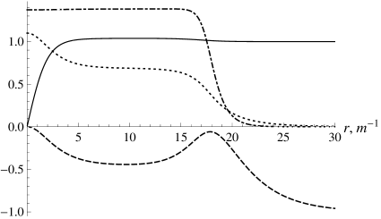
Figure 1: The numerical solution $m^{-1/2}A_{0}(r)/(er)$ (dotted), $A(r)$ (dashed), $F(r)$ (solid), and $m^{-1/2}\sigma(r)$ (dash-dotted) for the vortex-Q-ball system. The model’s parameters are $e=q=0.3\,m^{1/2}$, $\mu=0.5\,m$, $\lambda=0.335\,m$, $v=1.221\,m^{1/2}$, $g=1.0\,m$, $h=0.26$, and $N=1$. The phase frequency $\omega=0.38\,m$.

Any solution of field equations (9) – (11) is an extremum of the action $S=\int\mathcal{L}d^{2}xdt$. It is readily seen, however, that the Lagrangian density (1) does not depend on time if the field configurations are those of ansatz (23). It follows that any solution of system (24) – (27) is an extremum of the Lagrangian $L=\int\mathcal{L}d^{2}x$. Let $A_{0}(r)$, $A(r)$, $F(r)$, and $\sigma(r)$ be a solution of system (24) – (27) satisfying boundary conditions (29). After the scale transformation of the solution’s argument $r\rightarrow\lambda r$, the Lagrangian $L$ becomes a function of the scale parameter $\lambda$. The function $L\left(\lambda\right)$ has an extremum at $\lambda=1$, so its derivative with respect to $\lambda$ vanishes at this point: $\left.dL/d\lambda\right|_{\lambda=1}=0$. From this equation it follows that the virial relation holds for the vortex-Q-ball system:

$$2\left(E^{\left(E\right)}-E^{\left(H\right)}+E^{\left(P\right)}\right)+L^{\left(C\!S\right)}-\omega Q_{\chi}=0,$$ (42)

where

$$E^{\left(E\right)}=\frac{1}{2}\int E_{i}E_{i}d^{2}x=\pi\int_{0}^{\infty}\left(\left(\frac{A_{0}}{er}\right)^{\prime}\right)^{2}rdr$$ (43)

is the electric field’s energy,

$$E^{\left(B\right)}=\frac{1}{2}\int B^{2}d^{2}x=\pi\int_{0}^{\infty}\frac{A^{\prime}{}^{2}}{e^{2}r}dr$$ (44)

is the magnetic field’s energy,

$$E^{\left(P\right)}=2\pi\int_{0}^{\infty}\left[V\left(\left|\phi\right|\right)+U\left(\left|\chi\right|\right)\right]rdr$$ (45)

is the potential part of the soliton’s energy, and

$$L^{\left(C\!S\right)}=\frac{\mu}{4}\int\epsilon^{\rho\sigma\tau}F_{\rho\sigma}A_{\tau}d^{2}x$$ (46)

is the Chern-Simons part of the model’s Lagrangian.

4 Numerical results

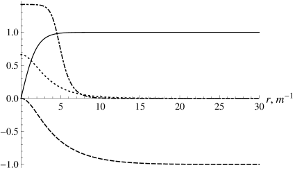
Figure 2: The numerical solution $m^{-1/2}A_{0}(r)/(er)$ (dotted), $A(r)$ (dashed), $F(r)$ (solid), and $m^{-1/2}\sigma(r)$ (dash-dotted) for the system of vortex and Q-ball that do not interact with each other. The model’s parameters are the same as in Fig. 1.

Now we present some numerical results concerning the vortex-Q-ball system. For numerical calculations, we use the natural units $c=1$, $\hbar=1$. In addition, the mass $m$ of scalar $\chi$-particle is used as the energy unit. After that, the model is completely determined by the seven parameters: $e$, $q$, $\mu$, $\lambda$, $v$, $g$, and $h$. We chose the following values of these parameters: $e=q=0.3\,m^{1/2}$, $\mu=0.5\,m$, $\lambda=0.335\,m$, $v=1.221\,m^{1/2}$, $g=1.0\,m$, and $h=0.26$, where the parameters’ dimensions correspond to the $(2+1)$-dimensional case. The correctness of the numerical solution were checked by use of Eqs. (13), (22), (41), and (42).

In Fig. 1, we can see the dimensionless zero component $m^{-1/2}A_{0}(r)/(er)$ of the gauge potential along with the dimensionless ansatz functions $A(r)$, $F(r)$, and $m^{-1/2}\sigma(r)$. The vortex part of the soliton system is in the topological sector with $N=1$, the phase frequency $\omega$ is equal to $0.38\,m$. Figure 2 presents the numerical solution for the case $q=0$, whereas the other model’s parameters remain the same as in Fig. 1. This corresponds to superimposed gauged vortex and non-gauged Q-ball that do not interact with each other. From Figs. 1 and 2, we can conclude that the gauge interaction between the vortex and Q-ball components leads to significant changes in the shapes of the ansatz functions $A_{0}(r)$, $A(r)$, and $\sigma(r)$, while the shape of $F(r)$ does not change significantly.

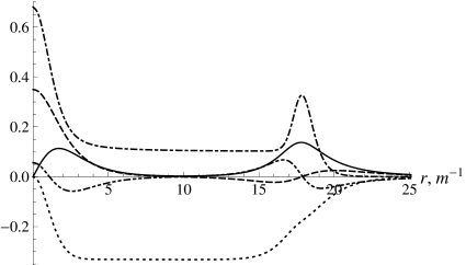
Figure 3: The dimensionless versions of the electric field strength $\tilde{E}_{r}(r)=m^{-3/2}E_{r}(r)$ (solid), the magnetic field strength $\tilde{B}(r)=m^{-3/2}B(r)$ (dashed), the scaled energy density $0.5\,\tilde{\mathcal{E}}(r)=0.5\,m^{-3}\mathcal{E}(r)$ (dash-dotted), the electric charge density $\tilde{j}_{0}(r)=m^{-5/2}j_{0}(r)$ (dash-dot-dotted), and the scaled angular momentum’s density $0.5\,\tilde{\mathcal{J}}(r)=0.5\,m^{-2}\mathcal{J}(r)$ (dotted), corresponding to the solution in Fig. 1.

Figure 3 shows the dimensionless versions of the electric field strength $\tilde{E}_{r}(r)=m^{-3/2}E_{r}(r)$, the magnetic field strength $\tilde{B}(r)=m^{-3/2}B(r)$, the scaled energy density $0.5\,\tilde{\mathcal{E}}(r)=0.5\,m^{-3}\mathcal{E}(r)$, the electric charge density $\tilde{j}_{0}(r)=m^{-5/2}j_{0}(r)$, and the scaled angular momentum’s density $0.5\,\tilde{\mathcal{J}}(r)=0.5\,m^{-2}\mathcal{J}(r)$ that correspond to the soliton solution in Fig. 1. We see that just as in [19], the vortex-Q-ball system consists of three parts: the central transition region, the inner region, and the external transition region. We also see that the densities of the energy and the angular momentum are approximately constant in the inner region, while the electric and magnetic field strengths are close to zero there.

In Fig. 4, we can see the dimensionless soliton energy $\tilde{E}=m^{-1}E$ as a function of the dimensionless phase frequency $\tilde{\omega}=m^{-1}\omega$. The function $\tilde{E}\left(\tilde{\omega}\right)$ is presented in the range from the minimum values of $\left|\tilde{\omega}\right|$ that we have reached by numerical methods to its maximum value of $1$. The most important feature of Fig. 4 is that the soliton’s energy is not invariant under the change of sign of the phase frequency: $\tilde{E}\left(-\tilde{\omega}\right)\neq\tilde{E}\left(\tilde{\omega}\right)$. This fact is a direct consequence of the $T$-invariance breaking, which is caused by the Chern-Simons term in the Lagrangian (1). From Fig. 4 it follows that the soliton’s energy $E$ tends to infinity as $\left|\tilde{\omega}\right|$ tends to its minimum values (thin-wall regime). In the thin-wall regime, the spatial size of the soliton’s inner region increases indefinitely, so the main contribution to the soliton’s energy and angular momentum comes from this region.

Figure 4: The dimensionless soliton energy $\tilde{E}=m^{-1}E$ as a function of the dimensionless phase frequency $\tilde{\omega}=m^{-1}\omega$. The model’s parameters are the same as in Fig. 1.

As $\tilde{\omega}\rightarrow 1$, the vortex-Q-ball system goes into the thick-wall regime. As well as in the thin-wall regime, the soliton’s Noether charge $Q_{\chi}$ and energy $E$ tend to infinity in the thick-wall regime. It was found numerically that $Q_{\chi}(\tilde{\omega})$ and $\tilde{E}(\tilde{\omega})$ have the following behaviour as $\tilde{\omega}\rightarrow 1$:

$$Q_{\chi}\underset{\tilde{\omega}\rightarrow 1}{\longrightarrow}B+A\left(1-\tilde{\omega}\right)^{-\frac{1}{2}},$$

$$\tilde{E}\underset{\tilde{\omega}\rightarrow 1}{\longrightarrow}C+A\left(2-\tilde{\omega}\right)\left(1-\tilde{\omega}\right)^{-\frac{1}{2}},$$ (47)

where $A$, $B$, and $C$ are positive constants. From Eq. (47) it follows that the behaviour of $Q_{\chi}\left(\tilde{\omega}\right)$ and $\tilde{E}\left(\tilde{\omega}\right)$ in the thick-wall regime is in agreement with Eq. (22). Such behaviour of $Q_{\chi}(\tilde{\omega})$ and $\tilde{E}(\tilde{\omega})$ in a neighborhood of the maximum value $\tilde{\omega}=1$ is very different from that of the two-dimensional non-gauged Q-ball [20]. It is also quite different from the behaviour of the vortex-Q-ball system [19] in the Maxwell gauge model. However, the behaviour of $Q_{\chi}(\tilde{\omega})$ and $\tilde{E}(\tilde{\omega})$ in a neighborhood of $\tilde{\omega}=1$ is similar to that of the usual three-dimensional Q-ball [20].

In Fig. 5, we can see the dependences of the dimensionless soliton energy $\tilde{E}$ and the absolute value of Noether charge $Q_{\chi}$ (which is negative for $\tilde{\omega}<0$) on the absolute value of $\tilde{\omega}$ in a neighborhood of $\left|\tilde{\omega}\right|=1$. From Fig. 5 it follows that the behaviour of the vortex-Q-ball system in the neighborhoods of $\tilde{\omega}=-1$ and $\tilde{\omega}=1$ is completely different. Indeed, its behaviour near $\tilde{\omega}=1$ corresponds to thick-wall regime (47). At the same time, its behaviour near $\tilde{\omega}=-1$ is rather unusual. Firstly, there is no thick-wall regime here. Secondly, the Q-ball component of the vortex-Q-ball system disappears at $\tilde{\omega}=-0.93$. For $\tilde{\omega}\in\left(-1,-0.93\right)$, we have only the single Maxwell-Chern-Simons vortex without any Q-ball component.

Figure 5: The dimensionless soliton energy $\tilde{E}=m^{-1}E$ (solid for $\tilde{\omega}>0$ and dash-dotted for $\tilde{\omega}<0$) and the absolute value of Noether charge $Q_{\chi}$ (dashed for $\tilde{\omega}>0$ and dotted for $\tilde{\omega}<0$) as functions of the absolute value of dimensionless phase frequency $\left|\tilde{\omega}\right|$ in a neighborhood of $\left|\tilde{\omega}\right|=1$.

Figure 6 shows the dimensionless energy $\tilde{E}$ as a function of the absolute value of Noether charge $Q_{\chi}$ for the both signs of $\tilde{\omega}$. It also shows the similar dependence $\tilde{E}\left(\left|Q_{\chi}\right|\right)$ for the two-dimensional non-gauged Q-ball with the same parameters $m$, $g$, and $h$ as for the vortex-Q-ball system. In addition, the straight line $\tilde{E}=\left|Q_{\chi}\right|$ is also shown in Fig. 6. We can see that the curve $\tilde{E}(\left|Q_{\chi}\right|)$ corresponding to the two-dimensional Q-ball is tangent to the straight line $\tilde{E}=\left|Q_{\chi}\right|$ at some nonzero $\left|Q_{\chi}\right|$ as it should be [20]. In contrast to this, the vortex-Q-ball system is described by the two curves, which correspond to the both signs of the phase frequency $\tilde{\omega}$. The curve $\tilde{E}(Q_{\chi})$ corresponding to the positive $\tilde{\omega}$ is similar to that of three-dimensional Q-ball. In particular, it has the cusp and consists of two branches. As $Q_{\chi}\rightarrow\infty$, the lower branch goes into the thin-wall regime, while the upper one goes into the thick-wall regime. At the same time, the curve $\tilde{E}(-Q_{\chi})$ corresponding to the negative $\tilde{\omega}$ has no cusp and consists of only one branch. The curve starts at $Q_{\chi}=0$ and goes into the thin-wall regime as $Q_{\chi}\rightarrow-\infty$. From Fig. 6, we can conclude that in the thin-wall regime the Q-ball component of the the vortex-Q-ball system is stable to the decay into the massive scalar $\chi$-particles.

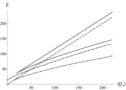
Figure 6: The vortex-Q-ball system’s dimensionless energy $\tilde{E}$ as a function of the absolute value of Noether charge $Q_{\chi}$ for $\tilde{\omega}>0$ (solid) and for $\tilde{\omega}<0$ (dash-dotted), and that for the two-dimensional non-gauged Q-ball (dash-dot-dotted) with the same parameters $m$, $g$, and $h$ as for the vortex-Q-ball system. The dashed line is the straight line $\tilde{E}=\left|Q_{\chi}\right|$.

5 Conclusions

In the present paper, we have researched the soliton system consisting of a vortex and a Q-ball that interact with each other through a common Abelian gauge field. Like a vortex, this two-dimensional soliton system has quantized magnetic flux (30). Due to the Chern-Simons term in the Lagrangian, the quantized magnetic flux leads to quantized electric charge (31) of the soliton system and, as a consequence, to a nonzero radial electric field. As a result, the soliton system possesses nonzero angular momentum (41) that depends linearly on the Noether charges of the scalar fields. Owing to the Chern-Simons term, the energy of the vortex-Q-ball system is not invariant under the sign reversal of the phase frequency $\omega$. This in turn leads to the significant change of the dependence $E(Q_{\chi})$ in comparison with the vortex-Q-ball system [19] and with the two-dimensional non-gauged Q-ball [20]. The vortex-Q-ball system combines properties of both nontopological (Eq. (22)) and topological (boundary condition (29) for $A(r)$ and, as a consequence, magnetic flux quantization (30)) solitons.

Finally, let us point out a possible application of the results obtained in [19] and in the present paper. A vortex-Q-ball string may arise when a cosmic string passes through a charged scalar condensate. Such a condensate could exist in the early universe; electrically charged boson stars [21], if they exist, also consist of such a condensate. A part of the condensate may be carried away by the passing cosmic vortex string, with the result that the vortex-Q-ball string arises. In this case, the gauge interaction between vortex and Q-ball components of the vortex-Q-ball string leads to significant changes of their properties.