Posterior inference unchained with EL₂O

Abstract

Statistical inference of analytically non-tractable posteriors is a difficult problem because of marginalization of correlated variables and stochastic methods such as MCMC and VI are commonly used. We argue that KL divergence minimization used by MCMC and stochastic VI is based on stochastic integration, which is noisy. We propose instead $t(\ln t)^{2}$ f-divergence, which evaluates expectation of L₂ distance squared between the approximate log posterior q and the un-normalized log posterior of p, both evaluated at the same sampling point, and optimizes on $q$ parameters. If $q$ is a good approximation to $p$ it has to agree with it on every sampling point and because of this the method we call EL₂O is free of sampling noise and has better optimization properties. As a consequence, increasing the expressivity of $q$ with point-wise nonlinear transformations and Gaussian mixtures improves both the quality of results and the convergence rate. We develop Hessian, gradient and gradient free versions of the method, which can determine M(M+2)/2+1, M+1 and 1 parameter(s) of $q$ with a single sample, respectively. EL₂O value provides a reliable estimate of the quality of the approximating posterior. We test it on several examples, including a realistic 13 dimensional galaxy clustering analysis, showing that it is 3 orders of magnitude faster than MCMC and 2 orders of magnitude faster than ADVI, while giving smooth and accurate non-Gaussian posteriors, often requiring dozens of iterations only.

Keywords: Approximate Bayesian Inference

1 Introduction

The goal of statistical inference from data can be stated as follows: given some data determine the posteriors of some parameters, while marginalizing over other parameters. The posteriors are best parametrized in terms of 1D probability density distributions, but alternative descriptions such as the mean and the variance can sometimes be used, especially in the asymptotic regime of large data where they fully describe the posterior. Occasionally we also want to examine higher dimensional posteriors, such as 2D probability density plots, but we rarely go to higher dimensions due to the difficulty of visualizing it. While we want to summarize the results in a series of 1D and 2D plots, the actual problem can have a large number of dimensions, most of which we may not care about, but which are correlated with the ones we do. The main difficulty in obtaining reliable lower dimensional posteriors lies in the marginalization part: marginals, i.e., averaging over the probability distribution of certain parameters, can change the answer significantly relative to the answer for the unmarginalized posterior, where those parameters are assumed to be known.

A standard approach to posteriors is Monte Carlo Markov Chain (MCMC) sampling. In this approach we sample all the parameters according to their probability density. After the samples are created marginalization is trivial, as one can simply count the 1D and 2D posterior density distribution of the parameter of interest. MCMC is argued to be exact, in the sense that in the limit of large samples it converges to the true answer. But in practice this limit may never be reached. For example, doing Metropolis sampling without knowing the covariance structure of the variables suffers from the curse of dimensionality. In very high dimensions this is practically impossible. One avoids the curse of dimensionality by having access to the gradient of the loss function, as in Hamiltonian Monte Carlo (HMC). However, in high dimensions thousands of model evaluations may be needed to produce a single independent sample (e.g. Jasche and Wandelt [2013]), which often makes it prohibitively expensive, specially if model evaluation is costly.

Alternatives to MCMC are approximate methods such as Maximum Likelihood Estimation (MLE) or its Bayesian version, Maximum A Posteriori (MAP) estimation, or KL divergence minimization based variational inference (VI). These can be less expensive, but can also give inaccurate results and must be used with care. MAP can give incorrect estimators in many different situations, even in the limit of large data, and is thus an inconsistent estimator, a result known since Neyman and Scott [1948]. Similarly, mean field VI can give an incorrect mean in certain situations. Full rank VI (FRVI) typically gives the posterior mean close to the correct value, but not always (we present one example in section 4). It often does not give correct variance. Quantifying the error of the approximation is difficult [Yao et al., 2018]. A related method is Population Monte Carlo (PMC) [Cappé et al., 2008, Wraith et al., 2009], which uses sampling from a proposal distribution to obtain new samples, and the posterior at the sample to improve upon the proposal sampling density. Both of these methods use KL divergence to quantify the agreement between the proposal distribution and the true distribution.

In many scientific applications the cost of evaluating the model and the likelihood can be very high. In these situations MCMC becomes prohibitively expensive. The goal of this paper is to develop a method that is optimization based and extends MAP and stochastic VI methods such as ADVI [Kucukelbir et al., 2017], such that it requires a low number of likelihood evaluations, while striving to be as accurate as MCMC. We would like to avoid some of the main pitfalls of the approximate methods like MAP or VI. Our goal is to have a method that works for both convex and non-convex problems, and works for moderately high dimensions, where a full rank matrix inversion is not a computational bottleneck: this can be a dozen or up to a few thousand dimensions, depending on the computational cost of the likelihood and the complexity of posterior surface.

The outline of the paper is as follows. In section 2 we compare traditional stochastic KL divergence approaches to our new proposal of using L₂ distance on a toy 1D Gaussian example. In section 3 we develop the method further by incorporating higher derivative information, and increasing the expressivity of approximate posteriors, while still allowing for analytic marginalization. In section 4 we show several examples, including a realistic data analysis example from our research area of cosmology. We conclude by discussion and conclusions in section 5.

2 Stochastic KL divergence minimization versus ${\bf EL_{2}O}$

A general problem of statistical inference is how to infer parameters from the data: we have some data $\hbox{\boldmath{$x$}}=\{x_{i}\}_{i=1}^{N}$ and some parameters the data depend on, $\hbox{\boldmath{$z$}}=\{z_{j}\}_{j=1}^{M}$. We want to describe the posterior of $z$ given data $x$. We can define the posterior $p(\hbox{\boldmath{$z$}}|\hbox{\boldmath{$x$}})$ as

$$p(\hbox{\boldmath{$z$}}|\hbox{\boldmath{$x$}})=\frac{p(\hbox{\boldmath{$x$}}|\hbox{\boldmath{$z$}})p(\hbox{\boldmath{$z$}})}{p(\hbox{\boldmath{$x$}})}=\frac{p(\hbox{\boldmath{$x$}},\hbox{\boldmath{$z$}})}{p(\hbox{\boldmath{$x$}})},$$ (1)

where $p(\hbox{\boldmath{$x$}}|\hbox{\boldmath{$z$}})$ is the likelihood of the data, $p(\hbox{\boldmath{$z$}})$ is the prior of $z$ and $p(\hbox{\boldmath{$x$}})=\int p(\hbox{\boldmath{$x$}}|\hbox{\boldmath{$z$}})p(\hbox{\boldmath{$z$}})d\hbox{\boldmath{$z$}}$ is the normalization. In general we have access to the prior and likelihood, but not the normalization. We can define the negative log of posterior in terms of what we have access to, which is negative log joint distribution $\tilde{\mathcal{L}}_{p}$, defined as

$$\tilde{\mathcal{L}}_{p}=-\ln p(\hbox{\boldmath{$x$}},\hbox{\boldmath{$z$}})=-\ln p(\hbox{\boldmath{$x$}}|\hbox{\boldmath{$z$}})-\ln p(\hbox{\boldmath{$z$}})=-\ln p(\hbox{\boldmath{$z$}}|\hbox{\boldmath{$x$}})-\ln p(\hbox{\boldmath{$x$}})\equiv\mathcal{L}_{p}-\ln p(\hbox{\boldmath{$x$}}).$$ (2)

For flat prior this is simply the negative log likelihood of the data. Note that the difference between $\tilde{\mathcal{L}}_{p}$ and $\mathcal{L}_{p}$ is $\ln p(\hbox{\boldmath{$x$}})$, which is independent of $z$, so in terms of gradients with respect to $z$ there is no difference between the two and we will not distinguish between them.

We would like to have accurate posteriors, but we would also like to avoid the computational cost of MCMC. Our goal is to describe the posteriors of parameters, and our approach will be rooted in optimization methods such as MAP or VI, where we assume a simple analytic form for the posterior, and try to fit its parameters to the information we have.

To explain the motivation behind our approach we will for simplicity in this section assume we only have a single parameter $z$ given the data $x$, $\tilde{\mathcal{L}}_{p}=-\ln p(z|\hbox{\boldmath{$x$}})+\ln p(\hbox{\boldmath{$x$}})$. We would like to fit the posterior of $z$ to a simple form, and the Gaussian ansatz is the simplest,

$$\mathcal{L}_{q}=-\ln q(z),\,q(z)=N(z;\mu,\Sigma).$$ (3)

We will also assume the posterior is Gaussian for the purpose of expectations, but since this is something we do not know a priori we will perform the estimation of parameters of $q$.

2.1 Stochastic KL divergence minimization

Many of the most popular statistical inference methods are rooted in the minimization of KL divergence, defined as

$${\rm KL}(q||p)=\operatorname{\mathbb{E}}_{q}(\mathcal{L}_{p}-\mathcal{L}_{q}),\,{\rm KL}(p||q)=\operatorname{\mathbb{E}}_{p}(\mathcal{L}_{q}-\mathcal{L}_{p}).$$ (4)

Here $\operatorname{\mathbb{E}}_{q}$, $\operatorname{\mathbb{E}}_{p}$ is the expectation over $q$ and $p$, respectively.

For intractable posteriors this cannot be evaluated exactly, and one tries to minimize KL divergence sampled over the corresponding probability distributions. Deterministic evaluation using quadratures is possible in very low dimensions or under the mean field assumption, but this becomes impossible in more than a few dimensions and we will not consider it further here. In this case stochastic sampling is the only practical method: we will thus consider stochastic minimization of KL divergence.

We first briefly show that stochastic minimization of ${\rm KL}(p||q)$ is noisy (this is a known result and not required for the rest of the paper). Let’s assume we have generated $N_{k}$ samples $z_{k}$ from $p$, using for example MCMC, with which we evaluate $\mathcal{L}_{p}(z_{k})$ for $k=1,..N_{k}$. We have

$${\rm KL}(p||q)=N_{k}^{-1}\left[\sum_{k}-\mathcal{L}_{p}(z_{k})+\frac{(z_{k}-\mu)^{2}}{2\Sigma}+\frac{\ln(2\pi\Sigma)}{2}\right].$$ (5)

Let us minimize ${\rm KL}(p||q)$ with respect to $\mu$ and $\Sigma$. We find that $\mathcal{L}_{p}(z_{k})$ do not enter into the answer at all, and we get

$$\mu=N_{k}^{-1}\sum_{k}z_{k},\,\Sigma=N_{k}^{-1}\sum_{k}(z_{k}-\mu)^{2}.$$ (6)

As expected this is the standard Monte Carlo (MC) result for the first two moments of the posterior given the MCMC samples from $p$. The answer converges to the true value as $N_{k}^{-1/2}$: one requires many samples for convergence. MCMC sampling usually requires many calls to $\tilde{\mathcal{L}}_{p}(z)$ before an independent sample of $z_{k}$ is generated, with the correlation length strongly dependent on the nature of the problem and the sampling method. If one instead tries to approximate the moments of $p$ one obtains Expectation Propagation method [Minka, 2001].

Now let us look at stochastic minimization of ${\rm KL}(q||p)$. This corresponds to Variational Inference (VI) [Wainwright and Jordan, 2008, Blei et al., 2016], which is argued to be significantly faster than MCMC. Here we assume $q$ is approximate posterior with a known analytic form, but since the posterior $p$ is not analytically tractable we will create samples from $q$ (an example of this procedure is ADVI, Kucukelbir et al. [2017]). Let us define the samples as

$$z_{k}=\Sigma^{1/2}\epsilon_{k}+\mu,$$ (7)

where $\epsilon_{k}$ is a random number drawn from a unit variance zero mean Gaussian $N(\epsilon_{k};0,1)$. With this we find

$${\rm KL}(q||p)=N_{k}^{-1}\sum_{k}\left[-\frac{\epsilon_{k}^{2}}{2}-\frac{\ln(2\pi\Sigma)}{2}+\mathcal{L}_{p}(z_{k})\right].$$ (8)

We want to use $\mathcal{L}_{p}(z_{k})$ to update information on the mean $\mu$, but it only enters via $z_{k}$ inside $\mathcal{L}_{p}(z_{k})$. So if we want to minimize KL divergence with respect to $\mu$ we have to propagate its derivative through $z_{k}$, the so called reparametrization trick [Kingma and Welling, 2013, Rezende et al., 2014].

To proceed let us assume that the posterior is given by a Gaussian

$$p(z|\hbox{\boldmath{$x$}})=N(z;\mu_{t},\Sigma_{t}),$$ (9)

where the subscripts $t$ denote true value. Since we are for now assuming that we do not have access to the analytic gradient, we will envision that the gradient with respect to the $\mu$ and $\Sigma$ parameters inside $z_{k}$ can be evaluated via a finite difference, evaluating $\nabla_{z}\mathcal{L}_{p}(z_{k})=[\mathcal{L}_{p}(z_{k}+\delta z_{k})-\mathcal{L}_{p}(z_{k})]/\delta z_{k})$. With $\nabla_{\mu}\mathcal{L}_{p}=\nabla_{z}\mathcal{L}_{p}(dz/d\mu)=\nabla_{z}\mathcal{L}_{p}$ we find that the gradient of KL divergence with respect to $\mu$ equal zero gives

$$\nabla_{\mu}{\rm KL}(q||p)=\sum_{k}\frac{(z_{k}-\mu_{t})}{\Sigma_{t}}=0,\,\mu=\mu_{t}-N_{k}^{-1}\sum_{k}\Sigma^{1/2}\epsilon_{k}.$$ (10)

Since the mean of $\epsilon_{k}$ is zero this will converge to the correct answer, but will be noisy and the convergence to the true value will be as $N_{k}^{-1/2}$.

To solve for the variance we similarly take a gradient with respect to $\Sigma$ and set it to zero,

$$\nabla_{\Sigma}{\rm KL}(q||p)=-\frac{1}{2\Sigma}+\sum_{k}\frac{\Sigma^{-1/2}\epsilon_{k}(z_{k}-\mu_{t})}{2\Sigma_{t}}=0,$$ (11)

with solution

$$\Sigma=\frac{N_{k}\Sigma_{t}}{\sum_{k}\left[\epsilon_{k}^{2}+(\mu-\mu_{t})\Sigma^{-1/2}\epsilon_{k}\right]}.$$ (12)

Note that this is really a quadratic equation in $\Sigma^{1/2}$, which may have multiple roots: minimizing stochastic ${\rm KL}(q||p)$ is not a convex optimization problem. Even if we have converged on $\mu=\mu_{t}$ rapidly so that we can drop the last term in the denominator and avoid solving this as a quadratic equation, we are still left with a fluctuating term $(\sum_{k}\epsilon_{k}^{2})^{-1}$. This expression also converges as $N_{k}^{-1/2}$ to the true value. As we iterate towards the correct solution we also have to vary $q$, so the overall number of calls to $\tilde{\mathcal{L}}_{p}(z_{k})$ will be larger. Results are shown in figure 1.

In summary, minimizing ${\rm KL}(p||q)$ and ${\rm KL}(q||p)$ with sampling is a noisy process, converging to the true answer with $N_{k}$ samples as $N_{k}^{-1/2}$. We will argue below this is a consequence of KL divergence integrand not being positive definite. In this context it is not immediately obvious why should stochastic VI be faster than MCMC, except that the prefactor for MCMC is typically larger, because the MCMC samples of $p$ are correlated, while VI samples drawn from $q$ are not (this is however somewhat offset by the fact that in stochastic VI one must also iterate on $q$).

2.2 EL₂O: Optimizing the expectation of L₂ distance squared of log posteriors

Minimizing KL divergence is not the only way to match two probability distributions. Recent work has argued that KL divergence objective function may not be optimal, and that other objective functions may have better convergence properties [Ranganath et al., 2016]. In this work we will also modify the objective function, but with the goal of preserving the expectation of KL divergence minimization in appropriate limits. A conceptually simple approach is to minimize the Euclidean distance squared between the true and approximate log posterior averaged over the samples drawn from some fiducial posterior $\tilde{p}$ close to the posterior $p$: this too will be zero when the two are equal, and will be averaged over $\tilde{p}$: as long as $\tilde{p}$ is close to $p$ this will provide approximately correct weighting for the samples. If the distance is not zero it will also provide an estimate of the error generated by $q$ not being equal to $p$, which can be reduced by improving on $q$. While current estimate for $q$ can be used for $\tilde{p}$, and iterate on it, we wish to separate its role in terms of sampling versus evaluating its log posterior, so we will always denote the sampling from $\tilde{p}$, even when this will mean sampling from the current estimate of $q$.

The proposal of this paper is to replace the stochastic KL divergence minimization with a simpler and (as we will show) less noisy ${\rm L_{2}}$ optimization. Since KL divergence enjoys many information theory based guarantees, we would also like this ${\rm L_{2}}$ optimization to reduce to KL divergence minimization in the high sampling limit, if $\tilde{p}=q$. We will show later that this is indeed the case. To be slightly more general, we can introduce expectation of ${\rm L_{n}}$ distance (to the power $n$) of log posterior between the two distributions,

$${\rm EL_{n}}(\tilde{p})=\operatorname{\mathbb{E}}_{\tilde{p}}\left(|\mathcal{L}_{q}-\mathcal{L}_{p}|^{n}\right),$$ (13)

where $\tilde{p}$ denotes some approximation to $p$. These belong to a larger class of f-divergences, $D_{f}(p,q)=\operatorname{\mathbb{E}}_{q}f(p/q)$, such that KL($p|q$) is for $f(t)=t\ln t$, while for ${\rm EL_{n}}(p)$ we have $f(t)=t|\ln t|^{n}$.

In this paper we will focus on $n=2$. We cannot directly minimize the $L_{2}$ distance because we do not know the normalization $\ln p(x)$, so instead we will minimize it up to the unknown normalization,

$${\rm EL_{2}O}(\tilde{p})=\operatorname*{arg\,min}_{\mu,\Sigma,\ln\bar{p}}\operatorname{\mathbb{E}}_{\tilde{p}}[(\mathcal{L}_{q}-\tilde{\mathcal{L}}_{p}-\ln\bar{p})^{2}],$$ (14)

where $\ln\bar{p}$ is an approximation to $\ln p(x)$ and is a free parameter to be minimized together with $\mu,\,\Sigma$. Later we will generalize this to higher order derivatives of $\mathcal{L}_{p}$, for which we do not need to distinguish between $\tilde{\mathcal{L}}_{p}$ and ${\mathcal{L}}_{p}$. The choice of $\tilde{p}$ defines the distance. We present first the version where $\tilde{p}=q$, since we know how to sample from it, later we will generalize it to other sampling proposals. However, we view the sampling distribution as unrelated to the hyper-parameters of $q$ we optimize for, even when $\tilde{p}=q$, so unlike ADVI we will not be propagating the gradients with respect to the samples $z_{k}$ inside $\mathcal{L}_{p}$. For the 1D Gaussian case we have

$${\rm EL_{2}O}(\tilde{p})=\operatorname*{arg\,min}_{\mu,\Sigma,\ln\bar{p}}N_{k}^{-1}\sum_{k}\left[\frac{(z_{k}-\mu)^{2}}{2\Sigma}-\tilde{\mathcal{L}}_{p}(z_{k})-c\right]^{2}.$$ (15)

where $c=\ln\bar{p}-(\ln 2\pi\Sigma)/2$ is a constant to be optimized together with $\mu$ and $\Sigma$. Note that we are not using equation 7 to simplify the first term: we are separating the role of $\tilde{p}$ as a sampling proposal, from $q$ as an approximation to $p$, even when $\tilde{p}=q$.

We see that equation 15 is a standard linear regression problem with polynomial basis up to quadratic order in $z$, and the linear parameters to solve are $c-\mu^{2}/2\Sigma$ for $z^{0}$, $\mu/\Sigma$ for $z$ and $-1/2\Sigma$ for $z^{2}$. If we have $N_{k}=3$ one can obtain the complete solution via normal equations of linear algebra (or a single Newton update if using optimization), and then transform these to determine $\mu$, $\Sigma$ and $\ln\bar{p}$, which are uniquely determined, and if $p$ is Gaussian ($\mathcal{L}_{p}$ quadratic) ${\rm EL_{2}O}$ is zero. If $N_{k}>3$ the problem is over-constrained: if $\mathcal{L}_{p}$ is quadratic in $z$ we are not gaining any additional information and ${\rm EL_{2}O}$ is still zero. In fact, in this case the three samples could have been drawn from any distribution. There is no sampling noise in minimizing ${\rm EL_{2}O}$ if $p$ is covered by $q$. The results of KL divergence minimization implemented by ADVI and EL₂O minimization are shown in figure 1.

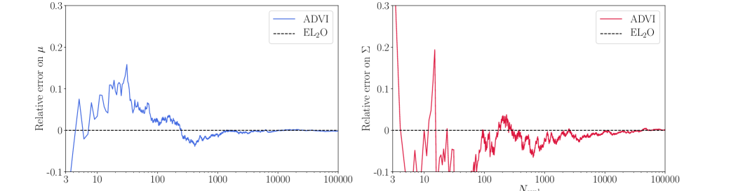
Figure 1: Relative errors on the mean $\mu$ and variance $\Sigma$ for the Gaussian ansatz of $q$ in a setting where $p$ is Gaussian. We find that the ADVI solution is noisy and only slowly converges to the correct answer, while EL₂O gives the exact solution after 3 evaluations, since there are 3 parameters to determine, after which the problem is over-determined.

If $\mathcal{L}_{p}$ is not quadratic then minimizing ${\rm EL_{2}O}$ finds the solution that depends on the class of functions $q$ and also on the samples drawn from $\tilde{p}$. In this case it is useful that the samples are close to the true $p$, since that means that we are weighting ${\rm EL_{2}O}$ according to the true sampling density (we will discuss the optimal choice of $\tilde{p}$ in section 4). Even in this situation however minimizing ${\rm EL_{2}O}$ has advantages. We will show below that the optimization is fast, more so if $q$ comes close to covering $p$. Moreover, the value of ${\rm EL_{2}O}$ at the minimum is informing us of the quality of the fit: if the fit is good and ${\rm EL_{2}O}$ is low we can be more confident of the resulting $q$ being a good approximation. If the fit is poor we may want to look for improvements in $q$. We will discuss several types of these that can reduce ${\rm EL_{2}O}$ beyond the full rank Gaussian approximation for $q$.

Even though we focus on ${\rm L_{2}}$ distance in this paper it is worth commenting on other distances. Of particular interest is ${\rm L_{1}}$ optimization defined as

$${\rm EL_{1}O}(\tilde{p})=\operatorname*{arg\,min}_{\mu,\Sigma,\ln\bar{p}}\operatorname{\mathbb{E}}_{\tilde{p}}(|\mathcal{L}_{q}-\tilde{\mathcal{L}}_{p}-\ln\bar{p}|).$$ (16)

If we use $\tilde{p}=q$ then this differs from ${\rm KL}(q||p)$ minimization only in taking the absolute value $|\mathcal{L}_{p}-\mathcal{L}_{q}|$ (in terms of f-divergence $t\ln t$ is replaced with $t|\ln t|$). The difference is that while minimizing ${\rm KL}(q||p)$ minimizes $\mathcal{L}_{p}$ regardless of the $z_{k}$ dependent part of $\mathcal{L}_{q}$, ${\rm EL_{1}O}$ tries to set it to $\mathcal{L}_{p}=\mathcal{L}_{q}$, up to the normalization $\ln\bar{p}$. For a finite number of samples the two solutions differ and the latter enforces the sampling variance cancellation, since the values of $\mathcal{L}_{q}$ and $\tilde{\mathcal{L}}_{p}$ are both evaluated at the same sample $z_{k}$. We see from this example that the noise in KL divergence can be traced to the fact that its integrand is not required to be positive, while it is for ${\rm EL_{1}O}$ and ${\rm EL_{2}O}$. While there are many f-divergences that have this property, ${\rm EL_{2}O}$ leads to identical equations as KL divergence minimization in the high sampling limit, so for the rest of the paper we will focus on ${\rm EL_{2}O}$ only.

While $t\ln t$ and $t\ln^{2}t$ f-divergence minimization seems very similar, they are fundamentally different optimization procedures. Minimization of KL divergence only makes sense in the context of the KL divergence integral $\int dzq(\ln q-\ln p)$ : it is only positive after the integration and one cannot minimize the integrand alone. Deterministic integration is only feasible in very low dimensions, and stochastic integration via Monte Carlo converges slowly, as $N_{k}^{-1/2}$. In contrast, minimizing EL₂O is based on comparing $\ln q(z_{k})$ and $\ln p(z_{k})$ at the same sampling points $z_{k}$: if the two distributions are to be equal they should agree at every sampling point, up to the normalization constant. There is no need to perform an integral and instead it should be viewed as a loss function minimization procedure: there is no stochastic integration noise.

3 Expectation with $\bf L_{2}$ optimization (EL₂O) method

In this section we generalize the EL₂O concept in several directions. An important trend in the modern statistics and machine learning (ML) applications in recent years has been the development of automatic differentiation (and Hessians) of the loss function $\mathcal{L}_{p}$. Gradients enable us to do gradient based optimization and sampling, which is the basis of recent successes in statistics and ML, from HMC to neural networks. Codes such as Tensorflow, PyTorch and Stan have been developed to obtain analytic gradients using backpropagation method. The key property of these tools is that often the calculational cost of the analytic gradient is comparable to the cost of evaluating the function itself: this is because the calculation of the function and its gradient share many components, such that the additional operations of the gradient do not significantly increase the overall cost. In some cases, such as the nonlinear least squares to be discussed below, a good approximation of the Hessian can be obtained using function gradients alone (Gauss-Newton approximation), so if one has the function gradient one also gets an approximation to the Hessian for free. When one has access to the gradients and Hessian it is worth taking advantage of this information for posterior inference.

Assume we have a general gradient expansion of log posterior around a sample $\hbox{\boldmath{$z$}}_{k}$,

$$\mathcal{L}_{p}(\hbox{\boldmath{$z$}}_{k}+\Delta\hbox{\boldmath{$z$}}_{k})=\sum_{n=0}^{\infty}\frac{1}{n!}\nabla^{n}_{\hbox{\boldmath{$z$}}}\mathcal{L}_{p}(\hbox{\boldmath{$z$}}_{k})(\Delta\hbox{\boldmath{$z$}}_{k})^{n},$$ (17)

where $\nabla^{n}_{\hbox{\boldmath{$z$}}}\mathcal{L}$ is $M^{n}$ dimensional tensor of higher order derivatives. For $n=0$ this the log posterior value, for $n=1$ this is its gradient vector and for $n=2$ this is its Hessian matrix.

We perform the same expansion for our approximate posterior $q(\hbox{\boldmath{$z$}},\hbox{\boldmath{$\theta$}})$,

$$\mathcal{L}_{q}(\hbox{\boldmath{$z$}}_{k}+\Delta\hbox{\boldmath{$z$}})=-\ln q(\hbox{\boldmath{$z$}}_{k}+\Delta\hbox{\boldmath{$z$}})=\sum_{n=0}^{\infty}\frac{1}{n!}\nabla^{n}_{\hbox{\boldmath{$z$}}}\mathcal{L}_{q}(\hbox{\boldmath{$z$}}_{k})(\Delta\hbox{\boldmath{$z$}})^{n}.$$ (18)

We assume that $q(\hbox{\boldmath{$z$}},\hbox{\boldmath{$\theta$}})$ has a simple form so that these gradients can be evaluated analytically, and that it depends on hyper-parameters $\theta$ we wish to determine. We will begin with a multivariate Gaussian assumption for $q(\hbox{\boldmath{$z$}})$ with mean $\mu$ and covariance $\Sigma$,

$$q(\hbox{\boldmath{$z$}})=N(\hbox{\boldmath{$z$}};\hbox{\boldmath{$\mu$}},\hbox{\boldmath{$\Sigma$}})=(2\pi)^{-N/2}\det\hbox{\boldmath{$\Sigma$}}^{-1/2}e^{-\frac{1}{2}(\hbox{\boldmath{$z$}}-\hbox{\boldmath{$\mu$}})^{T}\hbox{\boldmath{$\Sigma$}}^{-1}(\hbox{\boldmath{$z$}}-\hbox{\boldmath{$\mu$}})},$$ (19)

$$\mathcal{L}_{q}=\frac{1}{2}\left[\ln\det\hbox{\boldmath{$\Sigma$}}+(\hbox{\boldmath{$z$}}-\hbox{\boldmath{$\mu$}})^{T}\hbox{\boldmath{$\Sigma$}}^{-1}(\hbox{\boldmath{$z$}}-\hbox{\boldmath{$\mu$}})+N\ln(2\pi)\right].$$ (20)

To make the expansion coefficients dimensionless we can first scale $z_{i}$,

$$z_{i}\rightarrow\frac{z_{i}-\mu_{i}}{\Sigma_{ii}^{1/2}}.$$ (21)

While centering (subtracting $\mu_{i}$) is not required at this stage, we will use it when we discuss non-Gaussian posteriors later. This scaling can be done using some approximate $\Sigma_{ii}$ from $q$ that need not be iterated upon, so for this reason we will in general separate it from the iterative method of determining $q$. In practice we set the scaling $\Sigma_{ii}$ after the burn-in phase of iterations, when $q$ is typically determined by MAP and Laplace approximation.

The considerations in previous section, combined with the availability of analytic gradient expansion terms, suggest to generalize ${\rm EL_{2}O}$ to the form that is the foundation of this paper,

$${\rm EL_{2}O}=\operatorname*{arg\,min}_{\hbox{\boldmath{$\theta$}}}\operatorname{\mathbb{E}}_{\tilde{p}}\left\{N_{\rm der}^{-1}\sum_{n=0}^{n_{\rm max}}\sum_{i_{1},..i_{n}}\alpha_{n}\left[\nabla^{n}_{\hbox{\boldmath{$z$}}}\mathcal{L}_{q}(\hbox{\boldmath{$z$}})-\nabla^{n}_{\hbox{\boldmath{$z$}}}\mathcal{L}_{p}(\hbox{\boldmath{$z$}},\hbox{\boldmath{$\theta$}})\right]^{2}\right\},$$ (22)

where the averaging is done over the samples $\hbox{\boldmath{$z$}}_{k}$ drawn from $\tilde{p}$, and where we define, for $n=0$, $\mathcal{L}_{p}=\tilde{\mathcal{L}}_{p}+\ln\bar{p}$. The sum over index $i_{1}..i_{n}$ should be symmetrized, so for example for $n=2$ it is over $i_{1},i_{2}\geq i_{1}$. Here $N_{\rm der}$ is the total number of all the terms, while $n_{\rm max}$ is the largest order of the derivatives we wish to include. This equation combines three main elements: sampling from $\tilde{p}$, evaluation of the log posterior $\mathcal{L}_{p}$ and its derivatives at samples, analytic evaluation of the same for $\mathcal{L}_{q}$, and finally $L_{2}$ objective optimization to find the best fit parameters $\theta$. The latter involves evaluating another sequence of first (and second, if second order optimization is used) order gradients, this time with respect to $\theta$.

In equation 22 we have introduced the weight $\alpha_{n}$, which accounts for different weighting of different derivative order, so that for example each tensor element of a Hessian $\nabla_{z_{i}}\nabla_{z_{j}}\mathcal{L}_{p}$ can have a different weight to each vector element of a gradient $\nabla_{z_{i}}\mathcal{L}_{p}$, which can have different weight as each $\mathcal{L}_{p}$. Because of scaling in equation 21 the expression is invariant under reparametrization of $z$, and one can view each element of gradient and Hessian as one additional evaluation of $\mathcal{L}_{p}$, which should have equal weight. For example, one can view $\mathcal{L}_{p}$ and $\nabla_{z_{i}}\mathcal{L}_{p}$ using a finite difference expression of the gradient into an evaluation of two $\mathcal{L}_{p}$ at two independent samples. In this view equation 14 turns into equation 22. However, because we want the samples to be spread over sampling proposal $\tilde{p}$, it is suboptimal to have $N$ ”samples” at nearly the same point gives by the gradient information, and for this reason $\alpha_{0}>\alpha_{1}>\alpha_{2}$.

Equal weight can also be justified using the fact that different gradient order terms determine different components of $\theta$. In the context of a full rank Gaussian for $q$ we can think of the log likelihood determining an approximation to the normalization constant $\ln p(x)$, the gradient determining the means $\mu$, and the Hessian determining the covariance $\Sigma$, of which the latter two are needed for the posterior. We will in fact write the optimization equations below explicitly in the form where these terms are separated. Due to the sample variance cancellation a single sample evaluation suffices, but each additional evaluation of these variables can be used to improve the proposed $q$. For example, in a Gaussian mixture model for $q$, at each sample evaluation of the log posterior, its gradient and Hessian gives enough information to fit another full rank Gaussian mixture component. However, other weights may be worth exploring, such as downweighting the Hessian in situations where it is only approximate, as in the Gauss-Newton approximation discussed further below.

We will generally stop at $n_{\rm max}=2$, but in some circumstances having access to analytic gradients beyond the Hessian could be beneficial. We will see below that one of the main problems of full rank Gaussian variational methods is its inability to model the change of sign of Hessian off-diagonal elements, which can be described with the third order expansion ($n_{\rm max}=3$) terms. However, doing gradient expansion around a single point has its limitations: the shape of the posterior could be very different just a short distance away: there is no substitute for sampling over the entire probability distribution. Moreover, evaluations beyond the Hessian may be costly even if analytic derivatives are used. For this reason we will develop here three different versions depending on whether we have access to only $n_{\rm max}=0$ information, $n_{\rm max}=1$, or $n_{\rm max}=2$.

3.1 Gradient and Hessian version

For $n_{\rm max}=2$ we optimize

$${\rm EL_{2}O}=N_{M}^{-1}\operatorname*{arg\,min}_{\ln\bar{p},\hbox{\boldmath{$\mu$}},\hbox{\boldmath{$\Sigma$}}^{-1}}\operatorname{\mathbb{E}}_{\tilde{p}}\left\{\sum_{i,j\leq i}^{M}\left[\nabla_{z_{i}}\nabla_{z_{j}}\mathcal{L}_{q}-\nabla_{z_{i}}\nabla_{z_{j}}\mathcal{L}_{p}\right]^{2}+\sum_{i=1}^{M}\left[\nabla_{z_{i}}\mathcal{L}_{q}-\nabla_{z_{i}}\mathcal{L}_{p}\right]^{2}+[\mathcal{L}_{q}-\tilde{\mathcal{L}}_{p}-\ln\bar{p}]^{2}\right\},$$ (23)

where $N_{M}=M(M+3)/2+1$. In this section we will drop for simplicity the last term and optimization over $\ln\bar{p}$ since we do not need it ($q$ is already normalized). For a more general $q$ such as a Gaussian mixture model this term needs to be included, as discussed further below. There is additional flexibility in terms of how much weight to give to Hessian versus gradient information, which we will not explore in this paper.

We first need analytic gradient and Hessian information of $q(\hbox{\boldmath{$z$}})$. Taking the gradient of $\mathcal{L}_{q}$ in equation 20 with respect to $z$ gives

$$\nabla_{\hbox{\boldmath{$z$}}}\mathcal{L}_{q}=\hbox{\boldmath{$\Sigma$}}^{-1}(\hbox{\boldmath{$z$}}-\hbox{\boldmath{$\mu$}}).$$ (24)

The Hessian is obtained as a second derivative of $\mathcal{L}_{q}(\hbox{\boldmath{$z$}})$ with respect to $z$,

$$\nabla_{\hbox{\boldmath{$z$}}}\nabla_{\hbox{\boldmath{$z$}}}\mathcal{L}_{q}(\hbox{\boldmath{$z$}})=\hbox{\boldmath{$\Sigma$}}^{-1}.$$ (25)

Even if we have only a single sample we can expect the Hessian evaluated at the sample to determine $\Sigma$ (since it has no dependence on $\mu$), and with $\Sigma$ determined we can use its gradient to determine $\mu$ from equation 24. In this approach we can thus write the optimization solution of equation 23 as

$$\hbox{\boldmath{$\Sigma$}}^{-1}=\operatorname{\mathbb{E}}_{\tilde{p}}\left[\nabla_{\hbox{\boldmath{$z$}}}\nabla_{\hbox{\boldmath{$z$}}}\mathcal{L}_{p}\right]\approx N_{k}^{-1}\sum_{k=1}^{\rm N_{k}}\nabla_{{\hbox{\boldmath{$z$}}}}\nabla_{\hbox{\boldmath{$z$}}}\mathcal{L}_{p}(\hbox{\boldmath{$z$}}_{k}).$$ (26)

Applying the optimization of equation 22 with respect to $\mu$ and keeping the gradient terms only (i.e. dropping $n=0$ term, since $n=2$ term has no $\mu$ dependence) we find,

$$\operatorname{\mathbb{E}}_{\tilde{p}}[\nabla_{\hbox{\boldmath{$z$}}}\mathcal{L}_{p}(\hbox{\boldmath{$z$}})]=\hbox{\boldmath{$\Sigma$}}^{-1}(\operatorname{\mathbb{E}}_{\tilde{p}}[\hbox{\boldmath{$z$}}]-\hbox{\boldmath{$\mu$}}),$$ (27)

$$\hbox{\boldmath{$\mu$}}=-\hbox{\boldmath{$\Sigma$}}\operatorname{\mathbb{E}}_{\tilde{p}}[\nabla_{\hbox{\boldmath{$z$}}}\mathcal{L}_{p}(\hbox{\boldmath{$z$}})+\hbox{\boldmath{$z$}}]\approx N_{\rm k}^{-1}\sum_{k=1}^{\rm N_{k}}\left[-\hbox{\boldmath{$\Sigma$}}\nabla_{\hbox{\boldmath{$z$}}}\mathcal{L}_{p}(\hbox{\boldmath{$z$}}_{k})+\hbox{\boldmath{$z$}}_{k}\right].$$ (28)

Expectation of these equations has been derived in the context of variational methods [Opper and Archambeau, 2009], showing that the solution to ${\rm EL_{2}O}$ is the same as VI minimization of ${\rm KL}(q||p)$ in the high sample limit, if $\tilde{p}=q$. But there is a difference in the sampling noise if the number of samples is low: the presence of $\hbox{\boldmath{$z$}}_{k}$ at the end of equation 28 guarantees there is no sampling noise, and no such term appears in stochastic KL divergence based minimization. As we argued above, stochastic minimization of KL divergence has sampling noise, while minimizing ${\rm EL_{2}O}$ gives estimators in equations 26, 28 that are exact even for a single sample, under the assumption of the posterior belonging to the family of model posteriors $q(\hbox{\boldmath{$z$}})$: it does not even matter where we draw the sample. If the posterior does not belong to this family we need to perform the expectation in equations 26, 28, by averaging over more than one sample. There will be sampling noise, but the closer $q$ family is to the posterior $p$ the lower the noise. This will be shown explicitly in examples of section 4, where we test the method on $q$’s generalized beyond the full rank Gaussian. The residual ${\rm EL_{2}O}$ informs us when this is needed: if it is large it indicates the need to improve $q$, by going beyond the full rank Gaussian. The approach of this paper is to generalize $q$ until we find a solution with low residual ${\rm EL_{2}O}$ so that the posterior is reliable: in examples of section 4 this is reached approximately when ${\rm EL_{2}O}<0.2$.

Since the gradient and Hessian gives enough information to determine $\mu$ and $\Sigma$ we can convert this into an iterative process where we draw a few samples, even as low as a single sample only. Assume that at the current iteration the estimate is $\hbox{\boldmath{$\mu$}}_{t}$ and $\hbox{\boldmath{$\Sigma$}}_{t}$ and that we have drawn a single sample $\hbox{\boldmath{$z$}}_{1}$ from $q=N(\hbox{\boldmath{$z$}};\hbox{\boldmath{$\mu$}}_{t},\hbox{\boldmath{$\Sigma$}}_{t})$. We also evaluate the gradient $\nabla_{\hbox{\boldmath{$z$}}}\mathcal{L}(\hbox{\boldmath{$z$}}_{1})$ and Hessian, giving the following updates

$$\hbox{\boldmath{$\Sigma$}}^{-1}_{t+1}=\nabla_{\hbox{\boldmath{$z$}}}\nabla_{\hbox{\boldmath{$z$}}}\mathcal{L}(\hbox{\boldmath{$z$}}_{1}),$$ (29)

$$\hbox{\boldmath{$\mu$}}_{t+1}=-\hbox{\boldmath{$\Sigma$}}_{t+1}\nabla_{\hbox{\boldmath{$z$}}}\mathcal{L}(\hbox{\boldmath{$z$}}_{1})+\hbox{\boldmath{$z$}}_{1}.$$ (30)

With an update $\hbox{\boldmath{$\mu$}}_{t+1}$ we can draw a new sample and repeat the process until convergence. In this paper we are assuming that the Hessian inversion to get the covariance matrix and sampling from it via Cholesky decomposition is not a computational bottleneck. This would limit the method to thousands of dimensions if full rank description of all the variables is needed, and if the cost of evaluating $\mathcal{L}_{p}$ is moderate. Note that if we were doing MAP we would have assumed $q$ is a delta function with mean $\hbox{\boldmath{$\mu$}}_{t}$, in which case there is only one sample at $\hbox{\boldmath{$z$}}_{1}=\hbox{\boldmath{$\mu$}}_{t}$: the equation above becomes equivalent to a second order Newton’s method for MAP optimization. One obtains a full distribution in the full rank Gaussian approximation by evaluating the Hessian at the MAP estimate (Laplace approximation). The ${\rm EL_{2}O}$ method is a very simple generalization of the Laplace approximation and for a single sample has equal cost, as long as the cost of matrix inversion is low. Once we have approximately converged on $\mu$ (burn-in phase) we can average over more samples to obtain a more reliable approximation for both $\mu$ and $\Sigma$. This often gives a more reliable estimate of $\mu$ since it smooths out any small scale ruggedness in the posterior. Typically we find a few samples suffice for simple problems. When problems are not simple (and ${\rm EL_{2}O}$ remains high) it is better to increase the expressiveness of $q$ beyond the full rank Gaussian, as discussed below. Only the full rank Gaussian allows analytic marginalization of correlated variables: one inverts the Hessian matrix $\hbox{\boldmath{$\Sigma$}}^{-1}$ to obtain the covariance matrix $\Sigma$, and marginalization is simply eliminatation of the rows and columns of $\Sigma$ for the parameters we want to marginalize over (for proper normalization one also needs to evaluate the determinant of the remaining sub-matrix). We want to preserve this property for more general $q$ as well, and given the above stated property of full rank Gaussian two ways to do so are one-dimensional transforms and Gaussian mixtures, both of which will be discussed below.

Algorithm 1 Full rank Gradient and Hessian EL₂O

  Input: data $x_{i}$, size $N$

  Initialize parameters $z_{i}$: random sample from prior, size $M$

  Find MAP using optimization for initial $\mu$. Use Laplace for initial $q(\hbox{\boldmath{$z$}})=N(\hbox{\boldmath{$\mu$}},\hbox{\boldmath{$\Sigma$}})$.

  while EL₂O value has not converged do

     Draw a new sample $z_{N_{k}+1}$. Increase $N_{k}$ by 1.

     if Hessian available then

        $\hbox{\boldmath{$\Sigma$}}^{-1}=N_{k}^{-1}\sum_{k=1}^{\rm N_{k}}\nabla_{{\hbox{\boldmath{$z$}}}}\nabla_{\hbox{\boldmath{$z$}}}\mathcal{L}_{p}(\hbox{\boldmath{$z$}}_{k})$

     else

        $\hbox{\boldmath{$\mathcal{H}$}}=\sum_{k=1}^{\rm N_{k}}(\hbox{\boldmath{$z$}}_{k}-\hbox{\boldmath{$\mu$}})(\hbox{\boldmath{$z$}}_{k}-\hbox{\boldmath{$\mu$}})$

        $\hbox{\boldmath{$\Sigma$}}^{-1}=\hbox{\boldmath{$\mathcal{H}$}}^{-1}\sum_{k=1}^{\rm N_{k}}(\hbox{\boldmath{$z$}}_{k}-\hbox{\boldmath{$\mu$}})\nabla_{\hbox{\boldmath{$z$}}}\mathcal{L}(\hbox{\boldmath{$z$}}_{k})$

     end if

     $\hbox{\boldmath{$\mu$}}=N_{\rm k}^{-1}\sum_{k=1}^{\rm N_{k}}\left[-\hbox{\boldmath{$\Sigma$}}\nabla_{\hbox{\boldmath{$z$}}}\mathcal{L}_{p}(\hbox{\boldmath{$z$}}_{k})+\hbox{\boldmath{$z$}}_{k}\right]$

     Compute EL₂O

  end while

3.2 Gradient only and gradient free versions

We argued above that it is always beneficial to evaluate the Hessian, since together with the gradient this gives us an immediate estimate of $M(M+3)/2$ parameters, which can be chosen to be $\hbox{\boldmath{$\Sigma$}}^{-1}$ and $\mu$, and so we get a full rank $q$ with a single sample. Moreover, for nonlinear least squares and related problems evaluating the Hessian in Gauss-Newton approximation is no more expensive than evaluating the gradient. Suppose however that the Hessian is not available and we only have access to the gradients. This is for example the ADVI strategy [Kucukelbir et al., 2017], but let us look at what our approach gives. Specifically, we want to minimize

$${\rm EL_{2}O}=(M+1)^{-1}\operatorname*{arg\,min}_{\ln\bar{p},\hbox{\boldmath{$\mu$}},\hbox{\boldmath{$\Sigma$}}^{-1}}\operatorname{\mathbb{E}}_{\tilde{p}}\left[\sum_{i=1}^{M}\left\{\nabla_{z_{i}}\mathcal{L}_{q}-\nabla_{z_{i}}\mathcal{L}_{p}\right\}^{2}+\left\{\mathcal{L}_{q}-\tilde{\mathcal{L}}_{p}-\ln\bar{p}\right\}^{2}\right],$$ (31)

where again for simplicity of this section we will drop the last term and not optimize over $\ln p(\hbox{\boldmath{$x$}})$, since we do not need it. The first term on the RHS is called the Fisher divergence $F(q,p)$ if sampled from $q$ and $F(p,q)$ if sampled from $p$ [Hammad, 1978], and Jensen-Fisher divergence if averaged over the two [Sánchez-Moreno et al., 2012]. This shows the connection of the gradient part of ${\rm EL_{2}O}$ to the Fisher information.

First derivatives with respect to $\mu$ give equation 28. To evaluate it we need to determine $\Sigma$. To get the equation for $\Sigma$ we first derive its gradient $\nabla_{\hbox{\boldmath{$\Sigma$}}^{-1}}{\rm EL_{2}O}$, and its Hessian, $\hbox{\boldmath{$\mathcal{H}$}}=\nabla_{\hbox{\boldmath{$\Sigma$}}^{-1}}\nabla_{\hbox{\boldmath{$\Sigma^{-1}$}}}{\rm EL_{2}O}$,

$$\hbox{\boldmath{$\mathcal{H}$}}=\operatorname{\mathbb{E}}_{\tilde{p}}[(\hbox{\boldmath{$z$}}-\hbox{\boldmath{$\mu$}})(\hbox{\boldmath{$z$}}-\hbox{\boldmath{$\mu$}})]\approx\sum_{k=1}^{\rm N_{k}}(\hbox{\boldmath{$z$}}_{k}-\hbox{\boldmath{$\mu$}})(\hbox{\boldmath{$z$}}_{k}-\hbox{\boldmath{$\mu$}}).$$ (32)

We need $N_{k}=M+1$ gradients sampled at $\hbox{\boldmath{$z$}}_{k}$ for this matrix to be non-singular if $\mu$ is also determined from the same samples. Taking the first derivative of equation 31 with respect to $\hbox{\boldmath{$\Sigma$}}^{-1}$ gives

$$\hbox{\boldmath{$\Sigma$}}^{-1}=\hbox{\boldmath{$\mathcal{H}$}}^{-1}\operatorname{\mathbb{E}}_{\tilde{p}}\left[(\hbox{\boldmath{$z$}}-\hbox{\boldmath{$\mu$}})\nabla_{\hbox{\boldmath{$z$}}}\mathcal{L}\right]\approx\hbox{\boldmath{$\mathcal{H}$}}^{-1}\sum_{k=1}^{\rm N_{k}}(\hbox{\boldmath{$z$}}_{k}-\hbox{\boldmath{$\mu$}})\nabla_{\hbox{\boldmath{$z$}}}\mathcal{L}(\hbox{\boldmath{$z$}}_{k}).$$ (33)

We obtained a set of equations 28 and 33 that only use gradient information, but these are different from the ADVI equations [Kucukelbir et al., 2017]. In particular, our equations have sampling variance cancellation built in, and if $q$ covers $p$ they give zero error once we have drawn enough samples so that the system is not under-constrained. For $\tilde{p}=p$ the $L_{2}$ norm of equation 31 has also been proposed by Hyvärinen [2005] as a score matching statistic, but was rewritten through integration by parts into a form that does not cancel sampling variance, similar to ${\rm KL}(p||q)$.

Finally, if we have no access to gradients we can still apply the ${\rm EL_{2}O}$ method: to get all the full rank parameters we need to evaluate the loss function in $M(M+3)/2+1$ points, and then optimize

$${\rm EL_{2}O}=\operatorname*{arg\,min}_{\ln\bar{p},\hbox{\boldmath{$\mu$}},\hbox{\boldmath{$\Sigma$}}^{-1}}\operatorname{\mathbb{E}}_{\tilde{p}}\left[\left\{\tilde{\mathcal{L}}_{q}-\mathcal{L}_{p}-\ln\bar{p}\right\}^{2}\right],$$ (34)

where this time we also need to optimize for $\ln\bar{p}$ together with $\mu$ and $\Sigma$. These equations also incorporate the sampling variance cancellation.

Hybrid approaches are also possible: for example, we may have access to analytic first or second derivatives for some parameters, but not for others. In this case, one can design an optimization process that uses analytic gradients and Hessian components for some of the parameters, while relying on either numerical finite differences or gradient free approaches for the other parameters. More generally, some parameters may require expensive and slow evaluations (slow parameters) while others can be inexpensive (fast parameters). In this case, we can afford to do numerical gradients with respect to fast parameters and focus on development of analytic gradients for slow parameters. Another hybrid approach will be discussed in the context of Gauss-Newton approximation below, where we use the Hessian in the Gauss-Newton approximation for the covariance matrix $\Sigma$, and only the gradient for the remaining hyper-parameters of $q$.

3.3 Posterior expansion beyond the full rank Gaussian: bijective 1D transforms

So far we obtained the full rank VI solution with an iterative process which should converge nearly as rapidly as MAP. If the posterior is close to the assumed multi-variate Gaussian then this process converges fast, and only a few samples are needed. If there is strong variation between the Hessian elements evaluated at different sampling points then we know the posterior is not well described by a multi-variate Gaussian. In this case we may want to consider proposal functions beyond equation 19. However, a multi-variate Gaussian is the only correlated multi-variate distribution where analytic marginalization can be done by simply inverting the Hessian matrix. This is a property that we do not want to abandon. For this reason we will first consider one-dimensional transformations of the original variables $z$ in this subsection, and Gaussian mixtures in the next. Variable transformations need to be bijective so that we can easily go from one set of the variables to the other and back [Rezende and Mohamed, 2015]. Here we will use a very simple family of models that give rise to skewness and curtosis, which are the one-dimensional versions of the gradient expansion at third and fourth order.

Specifically, we will consider bijective transformations of the form $y_{i}(z_{i})$ such that

$$q(\hbox{\boldmath{$z$}})=N({\hbox{\boldmath{$y$}}};\hbox{\boldmath{$\mu$}},\hbox{\boldmath{$\Sigma$}})\Pi_{i}|J_{i}|,\,\,J_{i}=\frac{dy_{i}}{dz_{i}},$$ (35)

with $N({\hbox{\boldmath{$y$}}};\hbox{\boldmath{$\mu$}},\hbox{\boldmath{$\Sigma$}})$ given by equation 19. Under this form the marginalization over the variables is trivial. For example, marginalized posterior distribution of $z_{i}$ is
$q[z_{i}(y_{i})]=N({y_{i}};\mu_{i},\Sigma_{ii})|dy_{i}/dz_{i}|$, where $\Sigma_{ii}$ is the diagonal component of the covariance matrix, obtained by inverting the Hessian matrix $\hbox{\boldmath{$\Sigma$}}^{-1}$.

We would like to modify the variables $z_{i}$ such that the resulting posteriors can accommodate more of the variation of $\tilde{\mathcal{L}}_{p}$. In one dimension this would be their skewness and curtosis, which are indicated for example by the variation of the Hessian with the sample, but in higher dimensions we also want to accommodate variation of off-diagonal terms of the Hessian. In typical situations given the full rank solution and the scaling of equation 21 the posterior mass will be concentrated around $-1<z_{i}<1$, but the distribution may be skewed, or have more or less posterior mass outside this interval.

A very simple change of variable is $y_{i}=z_{i}+\frac{1}{2}\epsilon_{i}z_{i}^{2}+\frac{1}{6}\eta_{i}z_{i}^{3}$, where we assume $\epsilon_{i}$ and $\eta_{i}$ are both parameters that can be either positive or negative, but small such that the relation is invertible. In one dimension the log of posterior is, keeping the terms at the lowest order in $\epsilon_{i}$ and $\eta_{i}$, $2\mathcal{L}_{q}\approx c+z_{i}^{2}+\epsilon_{i}z_{i}^{3}+\frac{1}{3}\eta_{i}z_{i}^{4}...$ Viewed as a Taylor expansion we see that $\epsilon_{i}$ term determines the third order gradient expansion and $\eta_{i}$ the fourth order, both around $z_{i}=0$.

To make these expressions valid for larger values of $\epsilon_{i}$ and $\eta_{i}$ we promote the transformation into

$$y_{i}(z_{i})={\rm sinh}_{\eta}\left[\frac{\exp(\epsilon_{i}z_{i})-1}{\epsilon_{i}}\right],$$ (36)

where for $\epsilon_{i}=0$ the above is just $y_{i}(z_{i})={\rm sinh}_{\eta}z_{i}$ [Schuhmann et al., 2016]

$${\rm sinh}_{\eta}(x)=\begin{cases}\eta^{-1}{\rm sinh}(\eta x)&(\eta>0)\\ x&(\eta=0)\\ \eta^{-1}{\rm arcsinh}(\eta x)&(\eta<0).\end{cases}$$ (37)

These are bijective, but not guaranteed to give the required posteriors. We can however apply the transformations multiple times for a more expressive family of models. For small values of $\epsilon$ and $\eta$ equation 36 reduces to the Taylor expansion above. If the posteriors are multi-peaked then these transformations may not be sufficient, and Gaussian mixture models can be used instead, discussed below.

The gradient of $\mathcal{L}_{q}$ is

$$\nabla_{z_{i}}\mathcal{L}_{q}=\sum_{j}(\Sigma^{-1})_{ij}(y_{j}-\mu_{j})J_{i}-\frac{\nabla_{z_{i}}|J_{i}|}{|J_{i}|},$$ (38)

while the Hessian is

$$\nabla_{z_{i}}\nabla_{z_{j}}\mathcal{L}_{q}=(\Sigma^{-1})_{ij}J_{i}J_{j}+\left[\sum_{k}(\Sigma^{-1})_{ik}(y_{k}-\mu_{k})\nabla_{z_{i}}J_{i}-\frac{\nabla_{z_{i}}\nabla_{z_{i}}|J_{i}|}{|J_{i}|}+\left(\frac{\nabla_{z_{i}}|J_{i}|}{|J_{i}|}\right)^{2}\right]\delta_{ij}.$$ (39)

If the Hessian is varying with the samples $\hbox{\boldmath{$z$}}_{k}$ we have an indication that we need higher order corrections. With the gradient and Hessian at a single sample $\hbox{\boldmath{$z$}}_{1}$ we have the sufficient number of constraints, $M(M+3)/2$, to determine $\mu$ and $\hbox{\boldmath{$\Sigma$}}^{-1}$. If we evaluate these variables at another sample $\hbox{\boldmath{$z$}}_{2}$ we already have too many constraints to determine the additional $2M$ nonlinear transform variables, so the problem is overconstrained even with two drawn samples. This is the power of having access to the gradient and Hessian information: we converge fast both because we can use Newton’s method to find the solutions and because a few samples give us enough constraints.

3.4 Posterior expansion beyond the full rank Gaussian: Gaussian mixtures

A second non-bijective way that can extend the expressivity of posteriors while still allowing for analytic marginalizations is a Gaussian mixture model [Bishop et al., 1997]. Here we model the posterior as a weighted sum of several multi-variate Gaussians, each of which can have an additional 1D NL transform, as in equation 35,

$$q(\hbox{\boldmath{$z$}})=\sum_{j}w_{j}N({\hbox{\boldmath{$y$}}^{j}};\hbox{\boldmath{$\mu$}}^{j},\hbox{\boldmath{$\Sigma$}}^{j})\Pi_{i}\left|\frac{dy_{i}^{j}}{dz_{i}}\right|\equiv\sum_{j}w_{j}q^{j}(\hbox{\boldmath{$z$}}),$$ (40)

where $\sum_{j}w_{j}=1$. We can introduce the position dependent weights

$$w_{j}(\hbox{\boldmath{$z$}})=\frac{w_{j}q^{j}(\hbox{\boldmath{$z$}})}{q(\hbox{\boldmath{$z$}})}.$$ (41)

We can now derive the corresponding $\nabla_{\hbox{\boldmath{$z$}}}\mathcal{L}_{q}$ and $\nabla_{\hbox{\boldmath{$z$}}}\nabla_{\hbox{\boldmath{$z$}}}\mathcal{L}_{q}$. For example, if $\hbox{\boldmath{$y$}}=\hbox{\boldmath{$z$}}$ the gradient is

$$\nabla_{\hbox{\boldmath{$z$}}}\mathcal{L}_{q}=\sum_{j}w_{j}(\hbox{\boldmath{$z$}})\nabla_{\hbox{\boldmath{$z$}}}\mathcal{L}_{q}=\sum_{j}w_{j}(\hbox{\boldmath{$z$}})(\hbox{\boldmath{$\Sigma$}}^{j})^{-1}(\hbox{\boldmath{$z$}}-\hbox{\boldmath{$\mu$}}^{j}),$$ (42)

and is simply a weighted gradient of each of the Gaussian mixture components. The Hessian is

$$\nabla_{\hbox{\boldmath{$z$}}}\nabla_{\hbox{\boldmath{$z$}}}\mathcal{L}_{q}=\sum_{j}\left[\nabla_{\hbox{\boldmath{$z$}}}w_{j}(\hbox{\boldmath{$z$}})\nabla_{\hbox{\boldmath{$z$}}}\mathcal{L}_{q}+w_{j}(\hbox{\boldmath{$z$}})\nabla_{\hbox{\boldmath{$z$}}}\nabla_{\hbox{\boldmath{$z$}}}\mathcal{L}_{q}\right]$$ (43)

$$= \sum_{j}w_{j}(\hbox{\boldmath{$z$}})(\hbox{\boldmath{$\Sigma$}}^{j})^{-1}-\sum_{i}\sum_{j\neq i}\frac{w_{i}(\hbox{\boldmath{$z$}})w_{j}(\hbox{\boldmath{$z$}})}{w_{i}}\left[(\hbox{\boldmath{$\Sigma$}}^{j})^{-1}(\hbox{\boldmath{$z$}}-\hbox{\boldmath{$\mu$}}^{j})(\hbox{\boldmath{$\Sigma$}}^{i})^{-1}(\hbox{\boldmath{$z$}}-\hbox{\boldmath{$\mu$}}^{i})\right].$$

Once we have these expressions we can insert them into equation 22 and optimize against the parameters of $q(\hbox{\boldmath{$z$}})$. This is an optimization problem and requires iterative method to find the solution, but no additional evaluations of $\mathcal{L}_{p}$. While previously we did not use $\mathcal{L}_{p}$ itself since we did not need $c$, now we need to use this value as well, at it determines the weights $w_{j}$. With $\mathcal{L}_{p}$, its gradient and its Hessian we have enough data to determine one Gaussian mixture component per sample $\hbox{\boldmath{$z$}}_{k}$. Once we have constructed the full $q$, to analytically marginalize over some of $z$ we need to invert separately each of the matrices $(\hbox{\boldmath{$\Sigma$}}^{j})^{-1}$.

To summarize, there exist expressive posterior parametrizations beyond the full rank Gaussian that allow for analytic marginalizations and that can fit a broad range of posteriors. Gaussian mixture model can for example be used for a multi-modal posterior distribution, and a single evaluation with a Hessian can fit one component of the multi-variate Gaussian mixture model. One dimensional nonlinear transforms can be used to give skewness, curtosis and even multi-modality to each dimension.

3.5 Sampling proposals

We argued above that KL$(p||q)$ minimization leads to standard MC method, while minimizing KL$(q||p)$ gives VI method. ${\rm EL_{2}O}$ has more flexibility in terms of the choice of the sampling proposal $\tilde{p}$. We list some of these below, with some specific examples presented in section 4.

Sampling from $q$: If we sample from $\tilde{p}=q$ and minimize ${\rm EL_{2}O}$ we get results equivalent to VI in the large sample limit. While sampling from $q$, and iterating on it, is the simplest choice, it is not the only choice, and may not be the best choice either. One disadvantage is that the samples change as we vary $q$ during optimization, increasing the number of calls to $\mathcal{L}_{p}$. A second disadvantage is that in high dimensions sampling from the full rank Gaussian becomes impossible since the cost of Cholesky decomposition becomes prohibitive. We will address this problem elsewhere.

Sampling from $p$: one alternative is to sample from $p$ itself. This has the advantage that the samples do not need to change as we iterate on $q$, and if the cost of $\mathcal{L}_{p}$ is dominant this can be an attractive possibility. There are inference problems where sampling from $p$ is easy. An example are forward inference problems: suppose we know the prior distribution of $x$ and we would like to know the posterior of $\hbox{\boldmath{$z$}}=f(\hbox{\boldmath{$x$}})+\hbox{\boldmath{$n$}}$, where $f$ is some function and $n$ is noise. In this case we can create samples of $z$ drawn from $p$ simply by drawing samples of $x$ from its prior and $n$ from noise distribution and evaluating $\hbox{\boldmath{$z$}}=f(\hbox{\boldmath{$x$}})+\hbox{\boldmath{$n$}}$.

In most cases however sampling from $p$ is hard. One possibility is to create a number of true samples from $p$ using MCMC. This may be expensive, since there is a burn-in period that one needs to overcome first. We can use ${\rm EL_{2}O}$ optimization with $\tilde{p}=q$ for the burn-in phase to get to the minimum, and from there sampling can be almost immediate, but samples will be correlated, and often the correlation length can be hundreds or more. For modern methods like HMC sampling can be more efficient in traversing the posterior with a lower number of $\tilde{\mathcal{L}}_{p}$ calls, so this approach is worth exploring further.

Sampling from approximate $p$: since MCMC is expensive one can try cheaper alternatives. One possibility is to sample from an approximate posterior generated with the help of simulations. Suppose one generates a simulation where one knows the answer. One then performs the analysis as on the data, obtaining the point estimate on the parameters in terms of their best fit mean or mode (MAP). Since we know the truth for simulation we can create a data sample by adding the difference between the truth and the point estimate of the simulation to the point estimate of the data. This will give an approximation to the posterior distribution $p$ where each sample is completely independent. It will not be exact because of realization dependence of the posterior, and some of the samples may end up being very unlikely in the sense of having a very high $\tilde{\mathcal{L}}_{p}$. Additional importance sampling may be needed to improve this posterior further.

Another strategy is not to sample at all, but devise a deterministic algorithm to select the points where to evaluate $\mathcal{L}_{p}$. For example, given a MAP+Laplace solution one could select the points that are exactly a fixed fraction of standard deviation away from MAP for every parameter. This strategy has had some success in filtering applications, where it is called unscented Kalman filter (UKF, Julier and Uhlmann [2004]). Another option is deterministic quadratures, such as Gauss-Hermite integration. These deterministic approaches become very expensive in high dimensions.

Sampling from $q+p$: symmetric KL divergence is called Jensen-Shannon divergence, and we can similarly do the same for EL₂O. Since L₂ norm is already symmetric we just need to sample from $p+q$. This may have some benefits: if one samples from $p$ then there is no penalty for posterior densities $q$ which do not vanish where $p=0$. Conversely, if one samples from $q$ there is no penalty for situations where $p$ does not vanish while $q=0$. For example, there may be multiple posterior peaks in true $p$, but if we only found one we would never know the existence of the others. In both cases the difficulty arises because the normalization of $p$ is not accessible to us. The latter case is often argued to be more problematic suggesting sampling from $p$ should be used if possible. However, note that in the case of widely separated posterior peaks sampling from true $p$ using MCMC may not be possible either, as MCMC may not find all of the posterior peaks. In this case sampling from $q$ using multiple starting points with a Gaussian mixture for $q$ is a better alternative.

If both of these issues are a concern one can try to sample from both $q$ and from $p$, mixing the two types of samples. This will give us samples where $p=0$ but $q>0$, and where $q=0$ but $p>0$, if such regions exist. Another hybrid sampling $p+q$ method is, after the burn in, to iterate on $q$, sample from it, use it as a starting point for a MCMC sampling method with fast mixing properties (such as HMC) to move to another point, record the sample, update $q$, and repeat the process. The samples from $q$ may suffer from having too large values of $\tilde{\mathcal{L}}_{p}$, so a Metropolis style acceptance rate can be added to prevent this. It is worth emphasizing that the philosophy of this paper is to find $q$ that fits the posterior everywhere: both samples from $q$ and samples from $p$ should lead to ${\rm EL_{2}O}$ close to zero. and if $q$ covers $p$ we should always find this solution in the limit of large sampling density. These issues will be explored further in next section, where we show for specific examples that more expressive $q$ reduce the differences between sampling from $q$ versus sampling from $p$ or $q+p$.

3.6 Hessian for nonlinear least squares and related loss functions

One of the most common statistical analyses in science is a nonlinear least squares problem, which is a simple acyclic graphical model. One has some data vector $x$ and some model for the data $\hbox{\boldmath{$f$}}(\hbox{\boldmath{$z$}})$, which is nonlinear in terms of the parameters $z$. We also assume a known data measurement noise covariance matrix $N$, which can be dependent of the parameters $z$. One may add a prior for the latent variables in the form,

$$\tilde{\mathcal{L}}_{p}=\frac{1}{2}\left\{\hbox{\boldmath{$z$}}^{T}\hbox{\boldmath{$Z$}}^{-1}\hbox{\boldmath{$z$}}+[\hbox{\boldmath{$x$}}-\hbox{\boldmath{$f$}}(\hbox{\boldmath{$z$}})]^{T}\hbox{\boldmath{$N$}}^{-1}[\hbox{\boldmath{$x$}}-\hbox{\boldmath{$f$}}(\hbox{\boldmath{$z$}})]+\ln\det\hbox{\boldmath{$ZN$}}\right\},$$ (44)

where $Z$ is the prior covariance matrix of $z$ and we assumed the prior mean is zero (otherwise we also need to subtract out the prior mean from $z$ in the first term).

The Hessian in the Gauss-Newton approximation is

$$\operatorname{\mathbb{E}}_{\tilde{p}}[\nabla_{\hbox{\boldmath{$z$}}}\nabla_{\hbox{\boldmath{$z$}}}\mathcal{L}_{p}]\approx\hbox{\boldmath{$Z$}}^{-1}+\operatorname{\mathbb{E}}_{\tilde{p}}\left\{2{\rm tr}\left[\hbox{\boldmath{$N$}}^{-1}(\nabla_{\hbox{\boldmath{$z$}}}\hbox{\boldmath{$N$}})\hbox{\boldmath{$N$}}^{-1}(\nabla_{\hbox{\boldmath{$z$}}}\hbox{\boldmath{$N$}})\right]+(\nabla_{\hbox{\boldmath{$z$}}}\hbox{\boldmath{$f$}})^{T}\hbox{\boldmath{$N$}}^{-1}(\nabla_{\hbox{\boldmath{$z$}}}\hbox{\boldmath{$f$}})\right\},$$ (45)

where we dropped the second derivative terms of $f$ and $N$. The former term multiplies the residuals $\hbox{\boldmath{$x$}}-\hbox{\boldmath{$f$}}(\hbox{\boldmath{$z$}})$, which close to the best fit (i.e. where the posterior mass is concentrated) are oscillating around zero if the model is a good fit to the data. This suppresses this term relative to the first derivative term, which is always positive: in the Gauss-Newton approximation the curvature matrix is explicitly positive definite, and so is its expectation value over the samples. Clearly this is no longer valid if we move away from the peak, or we have a multi-modal posterior, since we have extrema that are saddle points or local minima and Gauss-Newton is a poor approximation there, so care must be exercised when using Gauss-Newton away from the global minimum. In our applications we use the Hessian to determine $\hbox{\boldmath{$\Sigma$}}^{-1}$, but we ignore it when evaluating nonlinear parameters $\epsilon$ and $\eta$. The cost of evaluating the Hessian under the Gauss-Newton approximation equals the cost of evaluating the gradient $\nabla_{\hbox{\boldmath{$z$}}}\mathcal{L}_{p}$, since it simply involves first derivatives of $f$ or $N$.

3.7 Range constraints

If a variable has a boundary then finding a function extremum may not be obtained by finding where its gradient is zero, but may instead be found at the boundary. In this case the posterior distribution is abruptly changed at the boundary, which is difficult to handle with Gaussians. The most common case is that a given variable is bounded to a one sided interval, or sometimes to a two-sided interval. There are two methods one can adopt, first one is a transformation to an unconstrained variable and second one is a reflective boundary condition.

Suppose for example that we have a constraint $z_{i}^{\prime}>a_{i}$, and we would like to have an unconstrained optimization that also transitions to the $z^{\prime}$ prior on a scale $\xi_{i}$ away from $a_{i}$. We can use

$$z_{i}=\xi_{i}\ln\left(e^{\frac{z_{i}^{\prime}-a_{i}}{\xi_{i}}}-1\right)$$ (46)

as our new variable [Kucukelbir et al., 2017]. This variable becomes $z_{i}^{\prime}$ for $z_{i}^{\prime}\gg a_{i}+\xi_{i}$ and $\xi_{i}\ln(z_{i}^{\prime}-a_{i})/\xi_{i}$ for $a_{i}<z_{i}^{\prime}\ll a_{i}+\xi_{i}$, so $z_{i}$ is now defined on the entire real interval with no constraint. If we want to preserve the probability and use the prior on original $z^{\prime}$ we must also include the Jacobian $J_{i}=|dz_{i}/dz_{i}^{\prime}|$, $p(z_{i})=p(z_{i}^{\prime})J_{i}^{-1}$. The presence of the Jacobian modifies the loss function. In our examples below we are including the Jacobian and we treat $\xi_{i}$ as another nonlinear parameter attached to parameter $z_{i}$ with a constraint, so that we optimize EL₂O with respect to it. A problem with this method is that posterior will always go to zero at $z_{i}^{\prime}\rightarrow a_{i}$, since the Gaussian goes to zero at large values. So even though this method can be quite successful in getting most of the posterior correct, it will artificially turn down to zero at the boundary. This is problematic, since it suggests the data exclude the boundary even if they do not.

Second approach to a boundary $z_{i}^{\prime}>a_{i}$ is to extend the range to $z_{i}^{\prime}<a_{i}$ using a reflective (or mirror) boundary condition across $z_{i}^{\prime}=a_{i}$, such that if $z_{i}^{\prime}<a_{i}$ then $\tilde{\mathcal{L}}_{p}(z_{i}^{\prime}-a_{i})=\tilde{\mathcal{L}}_{p}(a_{i}-z_{i}^{\prime})$. This leads to the non-bijective transformation of appendix A with $b_{i}=0$: we have $z_{i}^{\prime}$ defined on entire range and we model it with a sum of two mirrored Gaussians. Effectively this is equivalent to an unconstrained posterior analysis, where we take the posterior at $z_{i}^{\prime}<a_{i}$ and add it to $z_{i}^{\prime}>a_{i}$. It solves the problem of the unconstrained transformation method above, as the posterior at the boundary is not forced to zero, since it can be continuous and non-zero across the boundary $a_{i}$. The marginalization over this parameter remains trivial, since it is as if the parameter is not constrained at all. For the purpose of the marginalized posterior for the parameter itself, we must add the $z_{i}^{\prime}<a_{i}$ posterior to $z_{i}^{\prime}>a_{i}$ posterior. If the posterior mass is non-zero at $z_{i}^{\prime}=a_{i}$ then this will result in the posterior abruptly transitioning from a finite value to 0 at the boundary. This method can be generalized to a two sided boundary. In section 4 we will show an example of both methods.

3.8 Related Work

Our proposed divergence is in the family of f-divergences. Recently, several divergences have been introduced (e.g. Ranganath et al. [2016], Dieng et al. [2017]) to counter the claimed problems of KL divergence such as its asymmetry and exclusivity of $q$, but here we argue that with sufficiently expressive $q$ these problems may not be fundamental for EL₂O method. Expectations of EL₂O equations agree with VI expressions of [Opper and Archambeau, 2009].

Stochastic VI has been explored for posteriors in several papers, including ADVI Kucukelbir et al. [2017]. In direct comparison test we find it has a slower convergence than EL₂O. For $n=1$ the Fisher divergence minimization has been proposed by Hyvärinen [2005] as a score matching statistic, but was rewritten through integration by parts into a form that does not cancel sampling variance and has similar convergence properties as stochastic VI. Reducing sampling noise has also been explored more recently in Roeder et al. [2017] in a different context and with a different approach. Quantifying the error of the VI approximation has been explored in Yao et al. [2018], but using EL₂O value is simpler to evaluate.

NL transformations have been explored in terms of boundary effects in Kucukelbir et al. [2017]. Our NL transformations correspond more explicitly to generalized skewness and curtosis parameters, and as such are useful for general description of probability distributions. We employ analytic marginals to obtain posteriors and for this reason we only employ a single layer point-wise NL transformations, instead of the more powerful normalizing flows Rezende and Mohamed [2015]. More recently, Lin et al. [2019] also adopt GM and NL for similar purposes, also using Hessian based second order optimization (called natural gradient in recent ML literature).

4 Numerical experiments

In this section we look at several examples in increasing order of complexity.

4.1 Non-Gaussian correlated 2D posterior

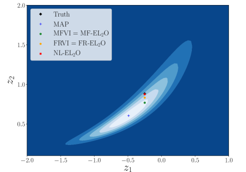
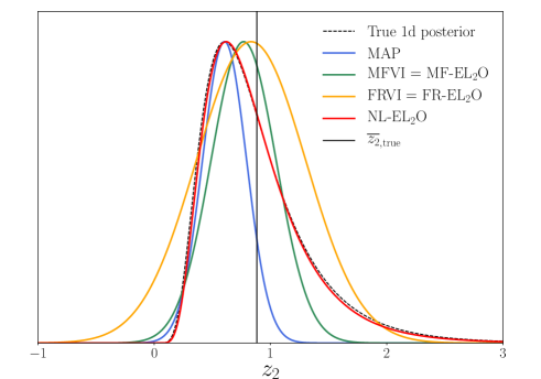
Figure 2: Example of a correlated non-Gaussian posterior problem, where one of the two Gaussian correlated variables $y_{2}$ is preceded by a nonlinear transformation (mapped by the exponential function, $z_{2}=\mathrm{exp}(y_{2})$). Left: The 2D posterior and the means estimated by various methods. Right: 1D marginalized posterior of $z_{2}$, with the black vertical line marking its true mean. MAP (blue) finds the mode and MFVI (green) FRVI (yellow) estimate the mean relatively well, but all of them fail to capture the correct shape of the posterior and its variance. Fitting for the skewness and curtosis parameters, EL₂O with the NL transform (NL-EL₂O, red) accurately models the posterior. All curves have been normalized to the same value at the peak to reduce their dynamical range.

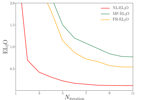
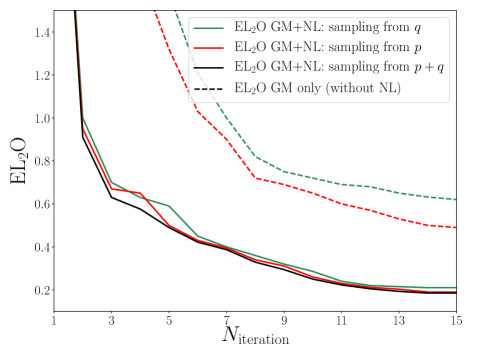
Figure 3: EL₂O values provide an estimate of the quality of the fit. Here we show them as a function of the number of iterations for the correlated non-Gaussian posterior example (Left panel) and for the forward model posterior example (Right panel). Typically values of EL₂O $\lesssim 0.2$ indicate that we have obtained a satisfactory posterior. The convergence is faster for NL-EL₂O despite having more parameters, a consequence of sampling noise free nature of EL₂O. In these examples each iteration draws 5 samples and we average over the past samples after the burn in. Right: Sampling from $p$ (red dashed) gives better EL₂O that sampling from $q$ (green dashed) for full rank GM. As we increase the expressivity of $q$, by applying the NL transform to better match the posterior, this makes EL₂O values for sampling from $p$ and $q$ more similar, and lower, improving the overall quality of the posterior.

In the first example we have a 2-dimensional problem modeled as two Gaussian distributed and correlated variables $z_{1}$ and $z_{2}$, but second one is nonlinear transformed using $\exp(z_{2})$ mapping. This transformation is not in the family of skewness and curtosis transformations proposed in section 3. Here we will try to model the posterior using $\epsilon$ and $\eta$ in addition to $\mu$ and $\Sigma$. The question is how well can our method handle the posterior of $z_{2}$, as well as the joint posterior of $z_{1}$ and $z_{2}$, and how does it compare to MAP, MF and FR VI or EL₂O.

The results are shown in figure 2. Left panel shows the 2D contours, which open up towards larger values of $z_{2}$ and as a result the MAP is away from the mean. Right hand panel shows the resulting posterior of MAP+Laplace, MF and FR EL₂O (which equals MFVI and FRVI in large sampling limit), and NL EL₂O. MAP gets the peak posterior correct but not the mean, MF improves on the mean and FR improves it further, but none of these get the full posterior. NL EL₂O gets the full posterior in nearly perfect agreement with the correct distribution, which is , 0.13 versus 0.5 or 0.7, respectively. What is interesting that the convergence of NL EL₂O is faster, despite having more parameters: the convergence has been reached after 8 iterations. We started with $N_{k}=1$ and ended with $N_{k}=5$ for this example. Note that we can reuse samples from previous iterations.

4.2 Forward model posterior

A very simple state evolution model is where we know the prior distribution of $x$, assumed to be a Gaussian with zero mean and variance $\Sigma$, and we would like to know the posterior of $z=x^{2}+n$, where $n$ is Gaussian noise with zero mean and variance $Q$. The loss function $\tilde{\mathcal{L}}_{p}$ is

$$\tilde{\mathcal{L}}_{p}=\frac{1}{2}\left[x\Sigma^{-1}x+(z-x^{2})Q^{-1}(z-x^{2})\right],$$ (47)

where we dropped all irrelevant constants. We would like to find the posterior of $z$ marginalized over $x$. In the absence of noise the problem can be solved using the Jacobian between $x$ and $z$, but addition of noise requires an additional convolution. In higher dimensions evaluating the Jacobian quickly becomes very expensive, so we will instead solve the problem by approximating the joint probability distribution of $x$ and $z$, and then marginalizing over $x$. This is a hard problem because the joint distribution is very non-Gaussian, as seen in figure 4.

We can first attempt to solve with MAP. The MAP solution is at $\hat{x}=\hat{z}=0$, and at the MAP Laplace approximation gives a diagonal Hessian between $x$ and $z$, so the two are uncorrelated. The variance on $z$ is $Q$, which vanishes in no noise $Q\rightarrow 0$ limit. MAP+Laplace for $z$ is thus a narrow distribution at zero, which is clearly a very poor approximation to the correct posterior.

The full rank VI or ${\rm EL_{2}O}$ approach is to sample from full rank Gaussian $q$ and iterate until convergence. The off-diagonal elements of the Hessian are given by $\nabla_{z}\nabla_{x}\mathcal{L}_{p}=-2xQ^{-1}$, which vanishes upon averaging over $x$, so full rank and mean field solutions are equal and FRVI assumes the two variables are uncorrelated. The variance on $z$ is again given by $Q$. The inverse variance of $x$ is $\nabla_{x}\nabla_{x}\mathcal{L}_{p}=\Sigma^{-1}+4x^{2}Q^{-1}$, which in ${\rm EL_{2}O}$ or VI we need to average over $q$. The stationary point is reached when $\operatorname{\mathbb{E}}[\nabla_{x}\nabla_{x}\mathcal{L}_{p}]^{-1}=\operatorname{\mathbb{E}}[x^{2}]=\sigma_{x}^{2}$, which in the low $Q$ limit gives $\sigma_{x}^{2}=Q^{1/2}/2$. Once we have the full rank Hessian we can also determine the means from the gradient of equation 47, finding a solution $\mu_{x}=\mu_{z}=0$. So we find a somewhat absurd result that even though $x$ is not affected by $z$ and its posterior should equal its prior, FRVI gives a different solution, one of a delta function at zero in the $Q\rightarrow 0$ limit, which is identical to the MAP solution. However, with this posterior the value of ${\rm EL_{2}O}$ is large, because the Hessian is fluctuating across the posterior and is not well represented with a single average. This is specially clear for the off-diagonal elements, whose average is zero, but the actual values fluctuate with rms of order $Q^{-3/4}$, very large fluctuations if $Q\rightarrow 0$.

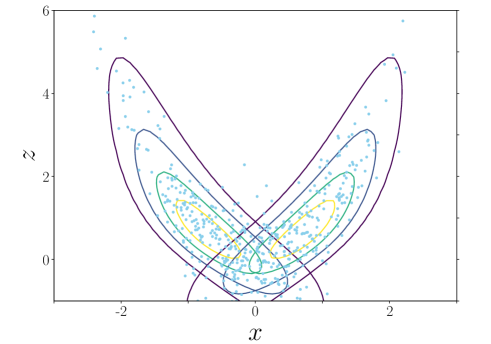
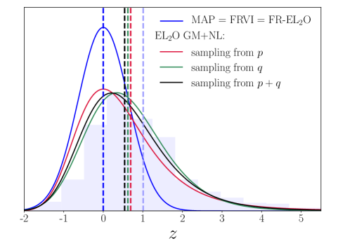
Figure 4: Example of a forward inference problem. Left: Contours of two symmetric Gaussian components (GM), with NL transform applied, together with samples from the posterior. The elliptical contours are warped by NL transform to better match the posterior. The total posterior is the sum of the two, which enhances the posterior density at $x\sim 0$. Right: 1D marginalized posterior of $z$ as approximated by different methods. MAP and FRVI (blue, normalized to the same peak value to reduce the dynamic range of the plot) give a poor estimate of posterior compared to MCMC (histogram). For EL₂O, we evaluated GM+NL with the following sampling proposals $\tilde{p}$: sampling from $p$ (red), $q$ (green), and $p+q$ (black). Note that sampling from $p$ is narrower than sampling from $q$. Vertical bars indicate the means, including MCMC (light blue dashed).

One must improve the model by going beyond a single full rank Gaussian. Here we will do so with a non-bijective transformation of appendix A, using $b_{x}=0$ and $a_{x}=0$, i.e. we model it as two Gaussian components mirror symmetric across $x=0$ axis. We use equation 43, which says that if the two Gaussian components are well separated the local Hessian can be used to determine $\hbox{\boldmath{$\Sigma$}}^{-1}$ of the local Gaussian component (which then also determines the covariance of the other component due to the symmetry). The local Hessian is given by $\nabla_{x}\nabla_{x}\mathcal{L}_{p}=\Sigma^{-1}+4\mu_{x}^{2}Q^{-1}$, $\nabla_{x}\nabla_{z}\mathcal{L}_{p}=-2\mu_{x}Q^{-1}$ and $\nabla_{z}\nabla_{z}\mathcal{L}_{p}=Q^{-1}$.

To further improve the model we consider bijective nonlinear transforms (NL). These are useful as they warp the ellipses, which allows to match $q$ closer to the true posterior $p$. The results are shown in figure 4. We see from the figure that MAP or FRVI=FR-EL₂O fail to give the correct posterior, while the Gaussian mixture with NL gives a very good posterior of $z$, in good agreement with MCMC.

In this example we can sample from $p$ directly, so we do not need to iterate on samples from $q$. ${\rm EL_{2}O}$ has flexibility to use samples from either of the two, which is distinctly different from KL based VI. This forward model problem gives us the opportunity to compare the results between the two. We would like to know if sampling from $q$ versus $p$ gives different answers, and if sampling from both further improves the results. This is also shown in figure 4. We see that there are some small differences in the posteriors, and that sampling from $q$ is slightly worse: in terms of ${\rm EL_{2}O}$ value, we get 0.20 for sampling from $p$ and $p+q$ and 0.23 for sampling from $q$. Somewhat surprising, we find that sampling from $q$ gives a broader approximation that sampling from $p$, contrary to KL divergence based FRVI [Bishop, 2007]. Sampling from $p+q$ does not further improve the results over sampling from $p$. The difference between $p$ and $q$ sampling is larger if we restrict to the full rank Gaussian without NL, and the ${\rm EL_{2}O}$ values are also larger: 0.4 for $p$ versus 0.5 for $q$. This suggests that while for simple $q$ the results may be biased and sampling from $p$ is preferred, more expressive $q$ reduces the difference between the two. This is not surprising: if $p$ is in the family of $q$ then we should be able to recover the exact solution with optimization, finding ${\rm EL_{2}O}=0$ upon convergence. If we want to improve the $q$ sampling results of figure 4 we can do so by adding additional Gaussian mixture components, or additional NL transforms, but we have not attempted to do so here.

A potential concern is that the exclusive nature of $q$ may lead to a situation where EL₂O sampled from $q$ is low, but the quality is poor, because $p>0$ where $q=0$. If this happens because there is another posterior maximum elsewhere far away then the only way to address it is using global optimization techniques like multiple starting points. All methods, including MCMC, have difficulties in these situations and require specialized methods (see below). If, on the other hand, there is excess posterior mass that is smoothly attached to the bulk of $q$ then EL₂O method should be able to detect it, specially with gradient and Hessian information. We can test it on this example by comparing EL₂O values on samples evaluated from $p$ versus samples evaluated from $q$, while using the same $\mathcal{L}_{q}$ to evaluate EL₂O. We find very little difference between the two, 0.24 versus 0.23, and so ${\rm EL_{2}O}$ evaluated on samples from $q$ gives a reliable estimate of the quality of solution. In these examples we used up to 15 iterations with $N_{k}=5$, and averaging over all past iterations after the burn-in.

4.3 Multi-modal posterior

Multi-modal posteriors are very challenging for any method. If the modes are widely separated then standard MCMC methods will fail, and specialized techniques, such as annealing or nested sampling [Handley et al., 2015] are required. If the modes are closer to each other so that their posteriors overlap then MCMC will be able to find them, and this is considered to be a strength of MCMC as compared to MAP or VI, which in the simplest implementations find only one of the modes. Here we use EL₂O with a Gaussian mixture (GM) on a simple bimodal posterior, which is a sum of two full rank Gaussians in 2 dimensions.

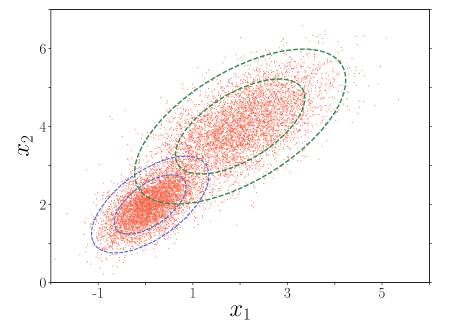
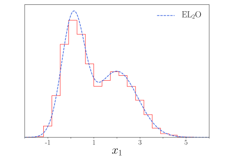
Figure 5: Application of a Gaussian mixture (GM) model to the multi-modal posterior problem. Left: Modeling the posterior as a weighted sum of two bivariate Gaussians, we demonstrate that the EL₂O method identifies both peaks, with means and covariances accurately estimated. A single starting point with 2 GM components converges to this solution after 15 iterations. For multiple starting points, each one converges within a few iterations to one of the two local minima, and EL₂O properly normalizes the two GM components. The two final solutions are identical (we show the multiple starting point method). Right: 1D marginalized posterior predicted by the EL₂O (blue dotted line), which closely matches the posterior from samples (red).

We show the results in figure 5. For this example we consider two optimization strategies. The first one is to first iterate on a full rank Gaussian, and since the residuals are large, we add a nonlinear transform. Since even after this residuals remain large we add a second Gaussian component. After a total of 13 iterations we converge to the correct posterior. This can be compared to Stein discrepancy method of Liu and Wang [2018], where 500 iterations with 100 particles were used to converge. The convergence to the correct result is possible because the two modes overlap in their posterior density.

The second strategy for these problems is to have multiple starting points. We will not discuss strategies how to choose the starting points, and we will adopt a simple random starting point method. In figure 5 we show results with several different starting points, each converging within a few iterations to one of two two modes (about half of the time onto each). How many starting points we need to choose depends on how many modes we discover: if after a few starting points we do not discover new modes we may stop the procedure. We construct the initial solution as the sum of the two Gaussians as found at each mode, using the gradient and Hessian to determine the full rank Gaussian, with the relative normalization determined by equation 34. If the two modes are widely separated this is already the correct solution, but in this case they are not and we use optimization to further improve on the initial parameters. The end result was identical to the above strategy, but the multiple starting points strategy is more robust, as it will find a solution even for the case of widely separated modes. In general, if multimodal posteriors are suspected (and even if not), multiple starting points are always recommended as a way to verify that optimization found all the relevant posterior peaks.

4.4 A science graphical model example: galaxy clustering analysis

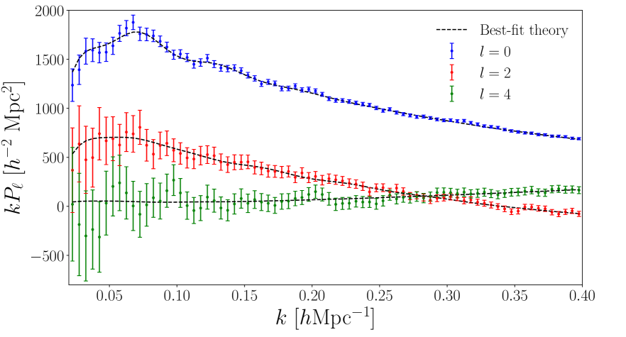
Figure 6: The power spectrum multipoles ($l=0,2,4$) from the best-fit theory model and measurements from the BOSS DR12 LOWZ+CMASS NGC data, with $0.4<z<0.6$. Fitting the model to data over the wavenumber range $k=0.02-0.4h$Mpc^-1, we find a good agreement between the model and the measurements.

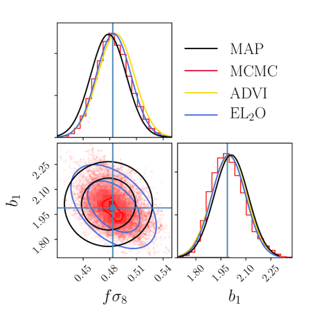
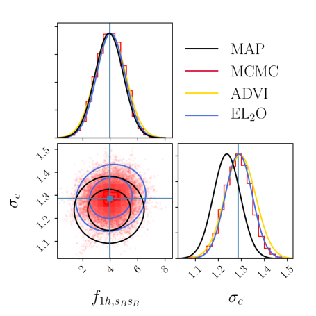
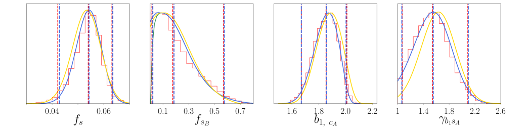
Figure 7: Top: 1D and 2D posterior distributions of four selected RSD model parameters whose posteriors are close to Gaussian. Top left panel: MAP+Laplace gives inaccurate 2D posterior relative to EL₂O, even if 1D projections are accurate. Top right panel: MAP can be displaced in the mean, while EL₂O and ADVI results agree very well with MCMC samples. Bottom: 1D posteriors for parameters which are most non-Gaussian. Together with the NL transform (blue solid curves), EL₂O results closely match the MCMC posterior (red solid). Also shown are 2.5%, 50%, and 97.5% intervals (dotted lines), for MCMC and EL₂O. 125 likelihood evaluations were used for EL₂O, compared to $10^{5}$ for MCMC, and $2.3\times 10^{4}$ for ADVI. Despite taking 200 times more steps than ${\rm EL_{2}O}$, ADVI posteriors are considerably worse. For $f_{sB}$ parameter we have a boundary $f_{sB}>0$, and we model it with the unconstrained transformation method (green solid) and adding the reflective boundary method to it, the latter allowing the posterior density at the boundary to be non-zero (blue solid).

Our main goal is a fast determination of posterior inference in a typical scientific analysis, where the model is expensive to evaluate, is nonlinear in its model parameters, and we have numerous nuisance parameters we want to marginalize over. Here we give an example from our own research in cosmology, which was the original motivation for this work, because MCMC was failing to converge for this problem. We observe about $10^{6}$ galaxy positions, measured out to about half of the lookback time of the universe and distributed over a quarter of the sky, with the radial position determined by their redshift extracted from galaxy spectroscopic emission lines. Galaxy clustering is anisotropic because of the redshift space distortions (RSD), generated by the Doppler shifts proportional to the galaxy velocities. We can summarize the anisotropic clustering by measuring the power spectrum as a function of the angle $\mu$ between the line of sight direction and the wavevector of the Fourier mode. In this specific case we are given measured summary statistics of galaxy clustering $\hat{P}_{l}(k)$, where $l=0,2,4$ are the angular multipoles (Legendre transforming the angular dependence on $\mu$) of the power spectrum and $k$ is the wavevector amplitude. We have a model prediction for the summary statistic $P_{l}(k)$ that depends on 13 different parameters, of which 3 are of cosmological interest, since they inform us of the content of the universe, including dark matter and dark energy. Others can be viewed as nuisance parameters, although they can also be of interest on their own [Hand et al., 2017]. We are also given the covariance matrix of the summary statistics (generalized noise matrix). The covariance matrix depends on the signal $P_{l}(k)$, so the derivative of the noise matrix with respect to the parameters needs to be included in the analysis. We assume flat prior on the parameters and we use Gauss-Newton approximation for the Hessian, so in terms of equation 44 we ignore the prior term with $S$, while the parameter dependence is both in $f$ and in $N$.

A common complication for scientific analyses is that the gradients are often not available in an analytic form: the models are evaluated as a numerical evaluation of ODEs or PDEs with many time steps to evolve the system from its initial conditions to the final output. Doing back-propagation on ODEs or PDEs with a large number of steps can be expensive and requires dedicated codes, which are often not available. In our application, we were able to do analytic derivatives for 9 parameters, leaving 4 to numerical finite difference method. We have implemented these with one sided derivatives (step size of 5%), meaning that we need 5 function calls to get the function and the gradient. Due to the use of Gauss-Newton approximation we also get an approximate Hessian at no extra cost. This finite difference approach could be improved, for example by using some more global interpolation schemes, but for this paper we will not attempt to do so.

Our specific optimization approach was to use L-BFGS (with L=5) for initial steps, switching to Gauss-Newton optimization at later steps closer to the solution. We started with assuming $q$ is a delta function (MAP approach), switching to sampling from $q$ as we approach the minimum, and gradually increasing the number of samples $N_{k}$ once we are past the burn-in, reusing samples from the previous iterations after the burn-in. Here burn-in is defined in terms of EL₂O not rapidly changing anymore. Overall it took 25 iteration steps to converge to the full non-Gaussian posterior solution. Number of samples and iteration steps used in all numerical examples are outlined in Table 1.

Results are shown in figure 7. In the top panel the parameters are $f\sigma_{8}$ (product of the growth rate $f$ and the amplitude of matter fluctuations $\sigma_{8}$), $b_{1}$ (linear bias), $\sigma_{c}$ (velocity dispersion for central galaxies), and $f_{1h,s_{B}s_{B}}$ (normalization parameter of the 1-halo amplitude). It is of interest to explore how it compares to MAP+Laplace (using Hessian of $\mathcal{L}_{p}$ at MAP to determine the inverse covariance matrix) in situations where the posterior is approximately Gaussian, and we show these results as well in the top panel of figure 7. We see that MAP+Laplace can fail in the mean, or in the covariance matrix. This could be caused by the marginalization over non-Gaussian probability distributions of other parameters, or caused by small scale noise in the log posterior close to the minimum, which EL₂O improves on by averaging over several samples. The results have converged to the correct posterior after 25 iterations, at which point the EL₂O value is stable and around 0.18, which we have argued is low enough for the posteriors to be accurate. Here we compare to MCMC emcee package [Foreman-Mackey et al., 2013], which initially did not converge, so we restarted it at the EL₂O best fit parameters (results are shown with $10^{5}$ samples after burn-in).

In the bottom panel we explore parameters that have the most non-Gaussian posteriors; these parameters are $f_{s}$ (satellite fraction), $f_{sB}$ (type B satellite fraction), both of which have positivity constraint, $b_{1,\ c_{A}}$ (linear bias of the type A central galaxies), and $\gamma_{b_{1}s_{A}}$ (slope parameter in the relation between $b_{1,\ s_{A}}$ and $b_{1,\ c_{A}}$). In all cases the EL₂O posteriors agree remarkably well with MCMC. This is even the case for the parameter $f_{sB}$, which has a positivity constraint $f_{sB}>0$, but is poorly constrained, with a very non-Gaussian posterior that peaks at 0. Even for this parameter the median and 2.5%, 97.5% lower and upper limits agree with MCMC. When we model this parameter with the unconstrained transformation method, we see that the probability rapidly descends to zero at the boundary $f_{sB}>0$. The reflective boundary method corrects this and gives a better result at the boundary, as also shown in the same figure. In this example, with reflective boundary, we allowed the posterior to go to -0.2 on this parameter. We do not show MAP+Laplace results since they poorly match these non-Gaussian posteriors.

	… Ex. 4.1…	…4.2…	…..4.3 …	…4.4…
$N_{k}$	1-10	1-10	1-10	1-10
$N_{\mathrm{iteration}}$	10	15	15	25
$N_{\rm tot}$	25	25	25	125

Table 1: Number of samples per iteration $N_{k}$, number of iteration steps $N_{\mathrm{iteration}}$, and total number of $\tilde{\mathcal{L}}_{p}$ evaluations (incldding burn-in) for 4 different numerical examples presented in this work. Example 4.4 does not have analytic gradients for 4 parameters, which are evaluated with a finite difference instead.

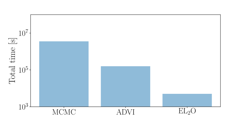
Figure 8: Timing results for 13-dimensional example of section 4.4. EL₂O is about 1000 times faster than MCMC and 200 times faster than ADVI using the same parametrization (but which did not converge to exact posteriors, as seen in figure 7).

5 Discussion and conclusions

The main goal of this work is to develop a method that gives reliable and smooth parameter posteriors, while also minimizing the number of calls to log joint probability $\tilde{\mathcal{L}}_{p}$. In many settings, specially for scientific applications, an evaluation of $\tilde{\mathcal{L}}_{p}$ can be extremely costly. The current gold standard are MCMC methods, which asymptotically converge to the correct answer, but require a very large number of likelihood evaluations, often exceeding $10^{5}$ or more. Scientific models are becoming more and more sophisticated, which comes at a heavy computational cost in terms of evaluation of $\tilde{\mathcal{L}}_{p}$. Using brute force MCMC sampling methods in these situations is practically impossible. In this paper we follow the optimization approaches of MAP+Laplace and stochastic VI [Kucukelbir et al., 2017], but we modify and extend these in several directions. The focus of this paper is on low dimensionality problems, where doing matrix inversion and Cholesky decomposition of the Hessian is not costly compared to evaluating $\tilde{\mathcal{L}}_{p}$. In practice this limits the method to of order thousands of parameters, if they are correlated so that the full rank matrix description is needed. If one can adopt sparse matrix approximations one can increase the dimensionality of the problem.

Both VI and MCMC methods rely on minimizing KL divergence. When the problem is not tractable using deterministic methods this minimization uses sampling, and this leads to a sampling noise in optimization that is only reduced as inverse square root of the number of samples. This can be traced to the feature of KL divergence that its integrand does not have to be positive, even if KL divergence is. minimization of KL divergence only makes sense in the context of the KL divergence integral $\int dzq(\ln q-\ln p)$ : it is only positive after the integration. Deterministic integration is only feasible in very low dimensions, and stochastic integration via Monte Carlo converges slowly, as $N_{k}^{-1/2}$. In this paper we propose instead to minimize ${\rm EL_{2}O}$, Euclidean L₂ distance squared between the log posterior $\mathcal{L}_{p}$, which we evaluate as $\tilde{\mathcal{L}}_{p}+\ln\bar{p}$, where $\ln\bar{p}$ is an unknown constant, and the equivalent terms of its approximation $\mathcal{L}_{q}$. EL₂O is based on comparing $\ln q(z_{k})$ and $\ln p(z_{k})$ at the same sampling points $z_{k}$: if the two distributions are to be equal they should agree at every sampling point, up to the normalization constant. There is no need to perform the integral to obtain a useful minimization procedure and there is no stochastic integration noise, only one extra optimization parameter due to the unknown normalization. When available we add its higher order derivatives, where we do not have to distinguish between $\mathcal{L}_{p}$ and $\tilde{\mathcal{L}}_{p}$. This is evaluated as expectation over some approximate probability distribution $\tilde{p}$ close to $p$. While one can construct many different f-divergences, ${\rm EL_{2}O}$ optimization agrees with KL divergence minimization based VI in the high sampling limit, if samples are generated from $\tilde{p}=q$. However, for a finite number of samples the resulting algorithm differs from recent VI methods such as ADVI [Kucukelbir et al., 2017], or the response method [Giordano et al., 2018]. While $t\ln t$ (KL divergence) and $t\ln^{2}t$ f-divergence minimization (EL₂O) seem very similar, they are fundamentally different, the former more related to stochastic integration.

A first advantage of ${\rm EL_{2}O}$ is that it has no sampling noise if the family of models $q$ covers $p$, in contrast to the stochastic minimization of KL divergence, as we demonstrate in section 2. In this case the method gives exact solution and ${\rm EL_{2}O}=0$, as long as we have enough constraints as the parameters, and it does not even matter where the samples are drawn from. In this limit additional samples make the problem over-constrained, which does not improve the result. If the family of $q$ is too simple to cover $p$ then the results fluctuate depending on the drawn samples and the convergence is slower. Having more expressive $q$ so that it is closer to $p$ makes the convergence faster even if there are more parameters to be determined. In practical examples we have observed this behavior once ${\rm EL_{2}O}$ dropped below 0.2 (e.g. figure 3), where we approach exact inference. This property of ${\rm EL_{2}O}$ is different from a stochastic KL divergence minimization, which is noisy and will typically take longer to converge as the number of paramaters increases. Moreover, as we argue in section 2, even in the simplest setting of Gaussian posterior stochastic KL divergence minimization is not a convex problem for a finite number of samples, while EL₂O is. In this setting EL₂O is not only convex, but also linear, so normal equations (or a single Newton update) give the complete solution. While we use L₂ distance in this paper, L₁ distance differs from KL divergence only in taking the absolute value of the log posterior difference, and also has no sampling noise. In terms of f-divergence ${\rm EL_{2}}$ corresponds to f-divergence $t(\ln t)^{2}$ and ${\rm EL_{1}}$ to $t|\ln t|$, in contrast to $t\ln t$ for KL divergence.

Second advantage of ${\rm EL_{2}O}$ is that its value can be used to quantify the quality of the solution: when it is small (less than 0.2 for our examples) $p$ is well described with $q$ and we may exit optimization. In contrast, in KL divergence based VI the value of the lower bound (ELBO) does not have an absolute meaning since it is related to the normalization $\ln p(x)$ (free energy bound, Jordan et al. [1999]): while relative changes of ELBO are meaningful, the absolute value is not and other methods are needed to assess the quality of the answer [Yao et al., 2018]. Even though we do not need it explicitly, EL₂O can easily optimize on and output an approximation to $\ln p(x)$. This can be useful for evidence or Bayes factor evaluations, which we will pursue elsewhere. Sometimes we find low EL₂O already for a full rank Gaussian and sometimes we need to go beyond it. There is not much computational benefit in using $q$ that is simpler than a full rank Gaussian, as long as Cholesky decomposition and matrix inversion are not a computational bottleneck: only the means are being optimized and not the covariance matrix elements. ${\rm EL_{2}O}$ value provides a diagnostic to asses the quality of the approximate posterior, so when it is large one can extend the family of models $q$ to remedy the situation. The strategy we advocate is to improve $q$ until a low value of ${\rm EL_{2}O}$ is reached. However, in contrast to recent trends in machine learning with many layers of nonlinear transformations (e.g. normalizing flows, Rezende and Mohamed [2015]), we advocate a single transformation with few parameters only, such that the number of $\tilde{\mathcal{L}}_{p}$ evaluations is minimized, and the analytic marginalization remains possible. If this fails to reduce EL₂O one can improve the approximate posterior by adding one Gaussian mixture or non-bijective transformation at a time.

Third advantage of ${\rm EL_{2}O}$ is its flexibility in choosing the sampling proposal $\tilde{p}$, which distinguishes it from the KL divergence based VI, which can only sample from $q$, and requires reparametrization trick for optimization [Kingma and Welling, 2013, Rezende et al., 2014]. This trick is not needed for ${\rm EL_{2}O}$ optimization. For $\tilde{p}$ one can use $q$, and iterate on it, which gives results identical to VI in the large sampling density limit. But we can also use true $p$ if we have a way to evaluate its samples, which is not only possible but easier than sampling from $q$ for forward model problems. We can also sample from both $p$ and $q$, which may avoid some of the pitfalls of the other sampling approaches.

Because we can choose different sampling proposals we can also address the quality of the results as a function of this choice. In the forward model example where sampling from $p$ is easy we have found that for simple $q$ (with ${\rm EL_{2}O}>0.4$) there was a difference between sampling from $q$ versus sampling from $p$, the latter giving overall better results. These differences were reduced as we increased the expressivity of $q$, for example when going from FR Gaussian to NL+FR, consistent with the statement above that more expressive $q$ improves the results and in the limit of very expressive $q$ we approach exact inference. Samples from $q$ and samples from $p$ gave nearly the same EL₂O value for the same $\mathcal{L}_{q}$, suggesting that sampling from $q$ may not be a fundamental limitation of EL₂O divergence based variational methods, but more a limitation of using insufficiently expressive forms of $q$. Recently, several divergences have been introduced (e.g. Ranganath et al. [2016], Dieng et al. [2017]) to counter these suggested problems of KL divergence, but here we argue that with sufficiently expressive $q$ this may not be an issue for EL₂O method. We also do not observe that in EL₂O sampling from $q$ leads to a significantly narrower approximation than sampling from $p$ once we go to NL+FR for $q$, in contrast to the arguments in the context of FRVI [Bishop, 2007]. In this example further improvement when sampling from $p+q$ was negligible. While this is based on a limited set of examples and deserves further study, we expect that with sufficiently expressive $q$ EL₂O value can be driven to zero and we approach exact inference, so that for most problems we only need to consider sampling from $\tilde{p}=q$.

Fourth advantage of ${\rm EL_{2}O}$ is its ability to use gradient and Hessian information (and even higher order derivatives if available), while preserving its sampling noise free nature. A significant trend in recent years, in machine learning, statistics and scientific computing, has been the development of analytic gradients and Hessians of $\tilde{\mathcal{L}}_{p}$ using methods such as backpropagation. ${\rm EL_{2}O}$ can take advantage of this and we present both the gradient based version and the gradient and Hessian based version. When ${\rm EL_{2}O}$ is using only the gradient information it can be related to Fisher divergence [Hammad, 1978]. The Hessian version converges especially rapidly, as every sample gives $M(M+3)/2+1$ constraints for $M$ dimensions, enough to fit a full rank Gaussian component in a Gaussian mixture model. Moreover, no optimization is needed to determine the covariance matrix of the Gaussian $q$, as its inverse is simply given by averaging the Hessian over the samples. When Hessian is not available one can use the gradient information as in equation 33 to achieve the same. For nonlinear least squares problems Hessian in the Gauss-Newton approximation can be obtained at the same cost as the gradient, and we found this approximation to give reliable posteriors in a realistic scientific application. For harder problems, where MAP, MFVI and FRVI with Gaussian $q$ all fail, we found the Gaussian mixture model to work well. In our applications we combine full rank Gaussian mixtures model with one dimensional nonlinear transforms to fit a general posterior, while at the same time also being able to do analytic marginalization over any parameters.

In most applications the number of iterations was comparable to the number of likelihood evaluations: we start with a single value for the mean MAP strategy for the burn in, then slowly increase the number of samples we average over by reusing samples from past iterations, typically to about 10-15 samples, if gradient and Hessian are available. In a realistic scientific application in the field of cosmology, with 13 parameters and no analytic derivatives for 4 of them, we obtained good posteriors with about 25 iterations, with 5 calls each to obtain the finite difference gradients, as compared to $10^{5}$ iterations for MCMC. This was a particularly difficult problem for MCMC, which did not even converge until we restarted it at ${\rm EL_{2}O}$ solution, and this problem was the original motivation for this work. Using the same parametrization on ADVI, with $2\times 10^{4}$ calls, we obtained worse posteriors despite 200 times higher computational cost, a consequence of noise in KL divergence it is minimizing. For many of the parameters the posteriors are very non-Gaussian, and we found remarkable agreement between ${\rm EL_{2}O}$ and MCMC using full rank Gaussian and a nonlinear transformation with two or three parameters for each dimension.

In this example evaluation of $10^{5}$ samples was feasible and we were able to compare the results to MCMC, but in many realistic situations MCMC would not even be feasible, and methods such as ${\rm EL_{2}O}$ may be one of the few possible alternatives. More generally, given the ubiquitousness of KL divergence in many applications in statistics and machine learning, ${\rm EL_{2}O}$ may also be useful as an alternative to KL divergence beyond the posterior inference applications described in this paper. One important application where EL₂O has an advantage over MCMC is calculation of normalization or evidence $p(x)$. As discussed in this paper, one of the optimization outputs of EL₂O procedure is $\ln\tilde{p}$, an approximation to $\ln p(x)$, which can in turn be used for model comparison by comparing the evidences between the different models.

6 Acknowledgments

We thank Andrew Charman, Yu Feng, Ryan Giordano, He Jia, Francois Lanusse, Patrick McDonald, Jeffrey Regier and Matias Zaldarriaga for useful discussions. US is supported by grants NASA NNX15AL17G, 80NSSC18K1274, NSF 1814370, and NSF 1839217.

References

- Jasche and Wandelt [2013] J. Jasche and B. D. Wandelt. Bayesian physical reconstruction of initial conditions from large-scale structure surveys. MNRAS, 432:894–913, June 2013. doi: 10.1093/mnras/stt449.
- Neyman and Scott [1948] J. Neyman and E. L. Scott. Consistent estimates based on partially consistent observations. Econometrica, 16:1–32, 1948.
- Yao et al. [2018] Yuling Yao, Aki Vehtari, Daniel Simpson, and Andrew Gelman. Yes, but did it work?: Evaluating variational inference. pages 5577–5586, 2018. URL http://proceedings.mlr.press/v80/yao18a.html.
- Cappé et al. [2008] Olivier Cappé, Randal Douc, Arnaud Guillin, Jean-Michel Marin, and Christian P. Robert. Adaptive importance sampling in general mixture classes. Statistics and Computing, 18(4):447–459, 2008. doi: 10.1007/s11222-008-9059-x. URL https://doi.org/10.1007/s11222-008-9059-x.
- Wraith et al. [2009] D. Wraith, M. Kilbinger, K. Benabed, O. Cappé, J.-F. Cardoso, G. Fort, S. Prunet, and C. P. Robert. Estimation of cosmological parameters using adaptive importance sampling. Phys. Rev. D, 80(2):023507, July 2009. doi: 10.1103/PhysRevD.80.023507.
- Kucukelbir et al. [2017] Alp Kucukelbir, Dustin Tran, Rajesh Ranganath, Andrew Gelman, and David M. Blei. Automatic differentiation variational inference. Journal of Machine Learning Research, 18:14:1–14:45, 2017. URL http://jmlr.org/papers/v18/16-107.html.
- Minka [2001] Thomas P. Minka. Expectation propagation for approximate bayesian inference. In UAI ’01: Proceedings of the 17th Conference in Uncertainty in Artificial Intelligence, University of Washington, Seattle, Washington, USA, August 2-5, 2001, pages 362–369, 2001. URL https://dslpitt.org/uai/displayArticleDetails.jsp?mmnu=1&smnu=2&article_id=120&proceeding_id=17.
- Wainwright and Jordan [2008] Martin J. Wainwright and Michael I. Jordan. Graphical models, exponential families, and variational inference. Foundations and Trends in Machine Learning, 1(1-2):1–305, 2008. doi: 10.1561/2200000001. URL https://doi.org/10.1561/2200000001.
- Blei et al. [2016] David M. Blei, Alp Kucukelbir, and Jon D. McAuliffe. Variational inference: A review for statisticians. CoRR, abs/1601.00670, 2016. URL http://arxiv.org/abs/1601.00670.
- Kingma and Welling [2013] Diederik P. Kingma and Max Welling. Auto-encoding variational bayes. CoRR, abs/1312.6114, 2013. URL http://arxiv.org/abs/1312.6114.
- Rezende et al. [2014] Danilo Jimenez Rezende, Shakir Mohamed, and Daan Wierstra. Stochastic backpropagation and approximate inference in deep generative models. In Proceedings of the 31th International Conference on Machine Learning, ICML 2014, Beijing, China, 21-26 June 2014, pages 1278–1286, 2014. URL http://jmlr.org/proceedings/papers/v32/rezende14.html.
- Ranganath et al. [2016] Rajesh Ranganath, Dustin Tran, Jaan Altosaar, and David M. Blei. Operator variational inference. In Advances in Neural Information Processing Systems 29: Annual Conference on Neural Information Processing Systems 2016, December 5-10, 2016, Barcelona, Spain, pages 496–504, 2016. URL http://papers.nips.cc/paper/6091-operator-variational-inference.
- Opper and Archambeau [2009] Manfred Opper and Cédric Archambeau. The variational gaussian approximation revisited. Neural Computation, 21(3):786–792, 2009. doi: 10.1162/neco.2008.08-07-592. URL https://doi.org/10.1162/neco.2008.08-07-592.
- Hammad [1978] P. Hammad. Mesure d’ordre α de l’information au sens de fisher. Revue de Statistique Applique ̵́e, 26:73–84, 1978.
- Sánchez-Moreno et al. [2012] P Sánchez-Moreno, A Zarzo, and J S Dehesa. Jensen divergence based on fisher’s information. Journal of Physics A: Mathematical and Theoretical, 45(12):125305, 2012. URL http://stacks.iop.org/1751-8121/45/i=12/a=125305.
- Hyvärinen [2005] Aapo Hyvärinen. Estimation of non-normalized statistical models by score matching. Journal of Machine Learning Research, 6:695–709, 2005. URL http://www.jmlr.org/papers/v6/hyvarinen05a.html.
- Rezende and Mohamed [2015] Danilo Jimenez Rezende and Shakir Mohamed. Variational inference with normalizing flows. In Proceedings of the 32nd International Conference on Machine Learning, ICML 2015, Lille, France, 6-11 July 2015, pages 1530–1538, 2015. URL http://jmlr.org/proceedings/papers/v37/rezende15.html.
- Schuhmann et al. [2016] R. L. Schuhmann, B. Joachimi, and H. V. Peiris. Gaussianization for fast and accurate inference from cosmological data. MNRAS, 459:1916–1928, June 2016. doi: 10.1093/mnras/stw738.
- Bishop et al. [1997] Christopher M. Bishop, Neil D. Lawrence, Tommi S. Jaakkola, and Michael I. Jordan. Approximating posterior distributions in belief networks using mixtures. In Advances in Neural Information Processing Systems 10, [NIPS Conference, Denver, Colorado, USA, 1997], pages 416–422, 1997. URL http://papers.nips.cc/paper/1392-approximating-posterior-distributions-in-belief-networks-using-mixtures.
- Julier and Uhlmann [2004] Simon J. Julier and Jeffrey K. Uhlmann. Unscented filtering and nonlinear estimation. Proceedings of the IEEE, 92(3):401–422, 2004. doi: 10.1109/JPROC.2003.823141. URL https://doi.org/10.1109/JPROC.2003.823141.
- Dieng et al. [2017] Adji Bousso Dieng, Dustin Tran, Rajesh Ranganath, John William Paisley, and David M. Blei. Variational inference via \chi upper bound minimization. In Advances in Neural Information Processing Systems 30: Annual Conference on Neural Information Processing Systems 2017, 4-9 December 2017, Long Beach, CA, USA, pages 2729–2738, 2017. URL http://papers.nips.cc/paper/6866-variational-inference-via-chi-upper-bound-minimization.
- Roeder et al. [2017] Geoffrey Roeder, Yuhuai Wu, and David K. Duvenaud. Sticking the landing: Simple, lower-variance gradient estimators for variational inference. In Advances in Neural Information Processing Systems 30: Annual Conference on Neural Information Processing Systems 2017, 4-9 December 2017, Long Beach, CA, USA, pages 6928–6937, 2017. URL http://papers.nips.cc/paper/7268-sticking-the-landing-simple-lower-variance-gradient-estimators-for-variational-inference.
- Lin et al. [2019] Wu Lin, Mohammad Emtiyaz Khan, and Mark W. Schmidt. Fast and simple natural-gradient variational inference with mixture of exponential-family approximations. In Proceedings of the 36th International Conference on Machine Learning, ICML 2019, 9-15 June 2019, Long Beach, California, USA, pages 3992–4002, 2019. URL http://proceedings.mlr.press/v97/lin19b.html.
- Bishop [2007] Christopher M. Bishop. Pattern recognition and machine learning, 5th Edition. Information science and statistics. Springer, 2007. ISBN 9780387310732. URL http://www.worldcat.org/oclc/71008143.
- Handley et al. [2015] W. J. Handley, M. P. Hobson, and A. N. Lasenby. POLYCHORD: next-generation nested sampling. MNRAS, 453:4384–4398, November 2015. doi: 10.1093/mnras/stv1911.
- Liu and Wang [2018] Qiang Liu and Dilin Wang. Stein variational gradient descent as moment matching. CoRR, abs/1810.11693, 2018. URL http://arxiv.org/abs/1810.11693.
- Hand et al. [2017] N. Hand, U. Seljak, F. Beutler, and Z. Vlah. Extending the modeling of the anisotropic galaxy power spectrum to k = 0.4 hMpc-1. J. Cosmology Astropart. Phys, 10:009, October 2017. doi: 10.1088/1475-7516/2017/10/009.
- Foreman-Mackey et al. [2013] D. Foreman-Mackey, D. W. Hogg, D. Lang, and J. Goodman. emcee: The MCMC Hammer. PASP, 125:306, March 2013. doi: 10.1086/670067.
- Giordano et al. [2018] Ryan Giordano, Tamara Broderick, and Michael I. Jordan. Covariances, robustness, and variational bayes. Journal of Machine Learning Research, 19, 2018. URL http://jmlr.org/papers/v19/papers/v19/17-670.html.
- Jordan et al. [1999] Michael I. Jordan, Zoubin Ghahramani, Tommi S. Jaakkola, and Lawrence K. Saul. An introduction to variational methods for graphical models. Machine Learning, 37(2):183–233, 1999. doi: 10.1023/A:1007665907178. URL https://doi.org/10.1023/A:1007665907178.