Towards machine learning in the
classification of $Z_{2}\times Z_{2}$ orbifold compactifications

Abstract

Systematic classification of $Z_{2}\times Z_{2}$ orbifold compactifications of the heterotic–string was pursued by using its free fermion formulation. The method entails random generation of string vacua and analysis of their entire spectra, and led to discovery of spinor-vector duality and three generation exophobic string vacua. The classification was performed for string vacua with unbroken $SO(10)$ GUT symmetry, and progressively extended to models in which the $SO(10)$ symmetry is broken to the $SO(6)\times SO(4)$, $SU(5)\times U(1)$, $SU(3)\times SU(2)\times U(1)^{2}$ and $SU(3)\times U(1)\times SU(2)^{2}$ subgroups. Obtaining sizeable numbers of phenomenologically viable vacua in the last two cases requires identification of fertility conditions. Adaptation of machine learning tools to identify the fertility conditions will be useful when the frequency of viable models becomes exceedingly small in the total space of vacua.

1 Introduction

String theory provides a viable framework to explore the synthesis of quantum mechanics with gravity. It gives rise to a multitude of phenomenological models that reproduce the main features of the Standard Model (SM), such as the presence of three generations with the correct gauge charges. A realistic string vacuum should reproduce the detailed structure of the Standard Model spectrum, including the masses of elementary particles and flavour mixing. A desirable property of phenomenological string vacua is the $SO(10)$ embedding of the SM states, which is motivated by the observed gauge charges and couplings. Existence of fundamental scalar doublets to facilitate electroweak symmetry breaking is indicated by the observation at the LHC of a scalar resonance compatible with the SM Higgs particle. The observed mechanism is compatible with a perturbative elementary coupling. Supersymmetrising the SM spectrum maintains the perturbative coupling up to the heterotic–string unification scale, thus enabling consistent perturbative unification of the Standard Model with gravity.

The caveat to the successful unified framework provided by string theory is the enormous number of potentially realistic string vacua. In the absence of clear indications from experiment for supersymmetry, or for any other extension of the SM that augments the electroweak symmetry breaking sector, the only method to constrain possible extensions of the SM is by fusing it with gravity. Otherwise, the SM may be augmented with an infinite number of continuous parameters. Synthesising the Standard Model with gravity therefore provides the only meaningful contemporary route to gain further insight into the basic properties of the fundamental matter and interactions. On the other hand, it should be also acknowledged that our current understanding of string theory is rudimentary and progress may take longer than that available for winning contemporary accolades. At present there is no concrete criteria that singles out a specific string vacuum, or particular class of string models, as phenomenologically preferable. Contemporary research in string phenomenology aims to explore large classes of string compactifications and their properties.

2 Realistic string models in the free fermionic formulation

Among the most realistic string models constructed to date are the heterotic–string models in the free fermionic formulation [1]. These models correspond to toroidal $Z_{2}\times Z_{2}$ orbifolds with discrete Wilson lines [2]. They produce an abundance of three generation models with various unbroken $SO(10)$ subgroups, including $SU(5)\times U(1)$ [3, 4]; $SO(6)\times SO(4)$ [5, 6]; $SU(3)\times SU(2)\times U(1)^{2}$ [7, 8]; $SU(3)\times U(1)\times SU(2)^{2}$ [9, 10], whereas the subgroup $SU(4)\times SU(2)\times U(1)$ does not produce viable models [11]. The free fermionic models produced the first known Minimal Standard Heterotic String Models (MSHSM) [7, 8] that give rise solely to the spectrum of the Minimal Supersymmetric Standard Model (MSSM) in the observable charged sector, and have been used to study many of the issues pertaining to the phenomenology of the Standard Model and unification [14]. Other classes of string compactifications are investigated [15].

In the free fermionic construction of the heterotic string in four dimensions all the extra degrees of freedom needed to cancel the conformal anomaly are represented as free fermions propagating on the two dimensional string worldsheet [1]. In the conventional notation the 64 lightcone gauge worldsheet fermions are denoted by:

   ${\underline{{\hbox{Left-Movers}}}}$:    $\psi^{\mu}_{1,2},~{}~{}~{}~{}{\chi_{i}},~{}~{}~{}~{}{y_{i},~{}~{}\omega_{i}}$    ${(i=1,\cdots,6)}$

   ${\underline{{\hbox{Right-Movers}}}}$:

$$~{}~{}~{}{\bar{\phi}}_{A=1,\cdots,44}~{}~{}=~{}~{}\begin{cases}~{}~{}{{\bar{y}}_{i}~{},~{}{\bar{\omega}}_{i}}&~{}~{}~{}{i=1,{\cdots},6}\cr&$ $\cr~{}~{}{{\bar{\eta}}_{i}}&~{}~{}~{}{U(1)_{i}~{}~{}~{}i=1,2,3{}{}}\cr~{}~{}{{\bar{\psi}}_{1,\cdots,5}}&~{}~{}~{}SO(10)$ $\cr~{}~{}{{\bar{\phi}}_{1,\cdots,8}}&~{}~{}~{}{SO(16)}$ $\end{cases}$$

where the six compactified coordinates of the internal manifold correspond to $\{y,\omega|{\bar{y}},{\bar{\omega}}\}^{1,\cdots,6}$ and the different symmetry groups generated by sixteen complexified right–moving fermions are indicated. String vacua in the free fermionic formulation are defined in terms of boundary condition basis vectors that denote the transformation properties of the fermions around the noncontractible loops of the worldsheet torus, and the Generalised GSO (GGSO) projection coefficients of the one loop partition function [1]. The free fermion models correspond to $Z_{2}\times Z_{2}$ orbifolds with discrete Wilson lines [2].

3 Realistic free fermionic models – old school

Three generation free fermionic models were constructed since the late eighties [3, 7, 5, 9]. The early models were built by following a trial and error method, using a common structure that underlined all the models, which consisted of a common set of five basis vectors known as the NAHE–set [13], denoted as $\{{\bf 1},S,b_{1},b_{2},b_{3}\}$. The gauge symmetry at the level of the NAHE–set is $SO(10)\times SO(6)^{3}\times E_{8}$, with forty–eight multiplets in the spinorial 16 representation of $SO(10)$, arising from the three twisted sectors of the $Z_{2}\times Z_{2}$ orbifold $b_{1}$, $b_{2}$ and $b_{3}$. The basis vector $S$ produces $N=4$ spacetime supersymmetry, which is broken to $N=2$ by the inclusion of $b_{1}$ and to $N=1$ by the inclusion of both $b_{1}$ and $b_{2}$. The action of $b_{3}$ either preserves or removes the remaining supersymmetry.

The second stage in the old school free fermionic model building consisted of augmenting the NAHE–set with three or four additional basis vectors. The basis vectors beyond the NAHE–set break the $SO(10)$ gauge group to one of its subgroups and simultaneously reduce the number of generations to three. In the standard–like models of [7] the additional basis vectors are denoted as $\{\alpha,\beta,\gamma\}$. They reduce the $SO(10)$ gauge symmetry to $SU(3)\times SU(2)\times U(1)_{B-L}\times U(1)_{R}$. and the weak hypercharge is given by the combination

$$U(1)_{Y}={1\over 2}(B-L)+T_{3_{R}}\in SO(10)!$$

Each of the sectors $b_{1}$, $b_{2}$ and $b_{3}$ gives rise to one generation which form complete 16 representations of $SO(10)$. The models contain the required scalar states to break the gauge symmetry further and to produce a quasi–realistic fermion mass spectrum [14].

4 Classification of fermionic $Z_{2}\times Z_{2}$ orbifolds – modern school

Since 2003 systematic classification of $Z_{2}\times Z_{2}$ orbifolds has been pursued by employing the free fermionic model building tools to derive and analyse the spectrum and leading coupling of these heterotic–string vacua. The initial classification method was developed in [16] for type II superstring. It was extended in [12] to string vacua with unbroken $SO(10)$ gauge group; and to vacua with: $SO(6)\times SO(4)$ subgroup in [6]; $SU(5)\times U(1)$ subgroup in [4]; $SU(3)\times SU(2)\times U(1)^{2}$ subgroup in [8]; $SU(3)\times U(1)\times SU(2)^{2}$ subgroup in [10]. In the free fermionic classification method the string vacua are generated by a fixed set of basis vectors, consisting of between twelve to fourteen basis vectors, $B=\{v_{1},v_{2},\dots,v_{14}\}.$ The models with unbroken $SO(10)$ gauge group are generated with a basis of twelve basis vectors

$$v_{1}={\bf 1} = \{\psi^{\mu},\ \chi^{1,\dots,6},y^{1,\dots,6},\omega^{1,\dots,6}~{}~{}~{}|~{}~{}~{}\bar{y}^{1,\dots,6},\bar{\omega}^{1,\dots,6},\bar{\eta}^{1,2,3},\bar{\psi}^{1,\dots,5},\bar{\phi}^{1,\dots,8}\},$$

$$v_{2}=S = \{\psi^{\mu},\chi^{1,\dots,6}\},$$

$$v_{3}=z_{1} = \{\bar{\phi}^{1,\dots,4}\},$$

$$v_{4}=z_{2} = \{\bar{\phi}^{5,\dots,8}\},$$ (1)

$$v_{4+i}=e_{i} = \{y^{i},\omega^{i}|\bar{y}^{i},\bar{\omega}^{i}\},\ i=1,\dots,6,~{}~{}~{}~{}~{}~{}~{}~{}~{}~{}~{}~{}~{}~{}~{}~{}~{}~{}~{}~{}~{}N=4~{}~{}{\rm Vacua}$$

$$v_{11}=b_{1} = \{\chi^{34},\chi^{56},y^{34},y^{56}|\bar{y}^{34},\bar{y}^{56},\bar{\eta}^{1},\bar{\psi}^{1,\dots,5}\},~{}~{}~{}~{}~{}~{}~{}~{}N=4\rightarrow N=2$$

$$v_{12}=b_{2} = \{\chi^{12},\chi^{56},y^{12},y^{56}|\bar{y}^{12},\bar{y}^{56},\bar{\eta}^{2},\bar{\psi}^{1,\dots,5}\},~{}~{}~{}~{}~{}~{}~{}~{}N=2\rightarrow N=1.$$

where the first ten basis vectors preserve $N=4$ spacetime supersymmetry and the last two correspond to the usual $Z_{2}\times Z_{2}$ orbifold twist. The third twisted sector is obtained as the basis vector combination $b_{3}=b_{1}+b_{2}+x$, where the $x$–sector arises as the basis vector combination

$$x={\bf 1}+S+\sum_{i=1}^{6}e_{i}+\sum_{k=1}^{2}z_{k}=\{{\bar{\psi}}^{1,\cdots,5},{\bar{\eta}}^{1,2,3}\}.$$ (2)

This vector combination plays an important role in the free fermionic systematic classification method as it induces a map between sectors that produce $SO(10)$ spinorial and vectorial representations. The breaking of the $SO(10)$ symmetry to the $SO(6)\times SO(4)$ subgroup is obtained by including in the basis the vector [6]

$$v_{13}=\alpha=\{\bar{\psi}^{4,5},\bar{\phi}^{1,2}\},$$ (3)

whereas the breaking to the $SU(5)\times U(1)$ subgroup is obtained with the vector [4]

$$v_{13}=\alpha=\{\overline{\psi}^{1,\dots,5}=\textstyle\frac{1}{2},\overline{\eta}^{1,2,3}=\textstyle\frac{1}{2},\overline{\phi}^{1,2}=\textstyle\frac{1}{2},\overline{\phi}^{3,4}=\textstyle\frac{1}{2},\overline{\phi}^{5}=1,\overline{\phi}^{6,7}=0,\overline{\phi}^{8}=0\,\},$$ (4)

and the breaking to the $SU(3)\times SU(2)\times U(1)^{2}$ is obtained by including both vectors in (3) and (4) as two separate vectors, $v_{13}$ and $v_{14}$ in the basis [8]. The breaking of the $SO(10)$ gauge symmetry to the $SU(3)\times U(1)\times SU(2)^{2}$ subgroup is achieved with the inclusion of the basis vector

$$v_{13}=\alpha=\{\overline{\psi}^{1,2,3}=\frac{1}{2}\;,\;\overline{\eta}^{1,2,3}=\frac{1}{2}\;,\;\overline{\phi}^{1,\ldots,6}=\frac{1}{2}\;,\;\overline{\phi}^{7}\}.$$ (5)

With a fixed set of boundary condition basis vectors the free fermionic classification method follows with variation of the GGSO projection coefficients. The general formula for the Generalised GSO (GGSO) projections on the states from a given sector $\xi$ is [1]

$${\rm e}^{i\pi(v_{j}\cdot F_{\xi})}|S\rangle_{\xi}=\delta_{\xi}C{\xi\atopwithdelims( )v_{j}}^{*}|S\rangle_{\xi}~{}.$$ (6)

The independent phases in a given string model can be enumerated in matrix form. For example, in the $SO(6)\times SO(4)$ models 66 phases are taken to be independent

$$\bordermatrix{&1&S&e_{1}&e_{2}&e_{3}&e_{4}&e_{5}&e_{6}&z_{1}&z_{2}&b_{1}&b_{2}&\alpha\cr 1&-1&-1&\pm&\pm&\pm&\pm&\pm&\pm&\pm&\pm&\pm&\pm&\pm\cr S~{}&&&-1&-1&-1&-1&-1&-1&-1&-1&1&1&-1\cr e_{1}~{}&&&&\pm&\pm&\pm&\pm&\pm&\pm&\pm&\pm&\pm&\pm\cr e_{2}~{}&&&&&\pm&\pm&\pm&\pm&\pm&\pm&\pm&\pm&\pm\cr e_{3}~{}&&&&&&\pm&\pm&\pm&\pm&\pm&\pm&\pm&\pm\cr e_{4}~{}&&&&&&&\pm&\pm&\pm&\pm&\pm&\pm&\pm\cr e_{5}~{}&&&&&&&&\pm&\pm&\pm&\pm&\pm&\pm\cr e_{6}~{}&&&&&&&&&\pm&\pm&\pm&\pm&\pm\cr z_{1}~{}&&&&&&&&&&\pm&\pm&\pm&\pm\cr z_{2}~{}&&&&&&&&&&&\pm&\pm&\pm\cr b_{1}~{}&&&&&&&&&&&&\pm&\pm\cr b_{2}~{}&&&&&&&&&&&&&\pm\cr\alpha~{}&&&&&&&&&&&&&\cr},$$

where the diagonal terms and below are fixed by modular invariance constraints. The remaining fixed phases are determined by imposing $N=1$ spacetime supersymmetry and the overall chirality of the chiral and supersymmetry generators. Varying the 66 phases randomly scans a space of $2^{66}$ (approximately $10^{19.9}$) $Z_{2}\times Z_{2}$ heterotic–string orbifold models. A particular choice of the 66, $\pm 1$ phases corresponds to a distinct string vacuum with massless and massive physical spectrum. The analysis proceeds by developing systematic tools to analyse the entire massless spectrum, as well as the leading top quark Yukawa coupling [18].

The power of the classification method is rooted in the structure of the set of basis vectors in eq. (1). The $Z_{2}\times Z_{2}$ orbifold has sixteen fixed points per twisted plane. Each of these fixed points can give rise to massless states in different representations of the unbroken four dimensional gauge group. The basis vectors in eq. (1) enables the analysis of the GGSO projection of each of these states individually. For example, states that arise in the 16 spinorial representation of $SO(10)$ are obtained from the $B_{pqrs}^{(1,2,3)}$ sectors given by

$${B_{pqrs}^{1}} = {S+b_{1}+pe_{3}+qe_{4}+re_{5}+se_{6}}$$

$$= \{\psi^{1,2},\chi^{1,2},(1-p)y^{3}{\bar{y}}^{3},p\omega^{3}{\bar{\omega}}^{3},(1-q)y^{4}{\bar{y}}^{4},q\omega^{4}{\bar{\omega}}^{4},$$

$$(1-r)y^{5}{\bar{y}}^{5},r\omega^{5}{\bar{\omega}}^{5},(1-s)y^{6}{\bar{y}}^{6},s\omega^{6}{\bar{\omega}}^{6},{\bar{\eta}}^{1},{\bar{\psi}}^{1,\cdots,5}\}$$

$${B_{pqrs}^{2}} = {S+b_{2}+pe_{1}+qe_{2}+re_{5}+se_{6}}$$

$${B_{pqrs}^{3}} = {S+b_{3}+pe_{1}+qe_{2}+re_{3}+se_{4}}$$

where $p,q,r,s=0,1$, whereas states that arise in the 10 vectorial representations of $SO(10)$ are obtained from the sectors $B_{pqrs}^{(1,2,3)}+x$, with the $x$–vector given in eq. (2). Thus, the initial classification was developed in [12] for sectors producing spinorial 16 and $\overline{\bf 16}$ representations and progressively extended to cover the entire Fock space. From the form of eq. (6) it is noted that whenever the overlap of periodic fermions in a sector $\xi$ and the vector $v_{j}$ is empty, the operator on the left side of the equation is positive. Hence, depending on the choice of the GGSO phase on the right side of eq. (6), the given state is either in or out of the spectrum. For example, for the spinorial representations from the twisted plane $B^{1}_{pqrs}$, and adopting the notation $C{{vi}\atopwithdelims[ ]{v_{j}}}~{}=~{}{\rm exp}[i\pi(v_{i}|v_{j})]$ with $(v_{i}|v_{j})=0,1$, we can assemble the projectors into an algebraic system of equations of the form

$$\Delta^{1}U^{1}_{\bf 16}=Y^{1}_{\bf 16}\Longleftrightarrow\left[\begin{array}[]{cccc}\left(e_{1}\left|e_{3}\right.\right)&\left(e_{1}\left|e_{4}\right.\right)&\left(e_{1}\left|e_{5}\right.\right)&\left(e_{1}\left|e_{6}\right.\right)\\ \left(e_{2}\left|e_{3}\right.\right)&\left(e_{2}\left|e_{4}\right.\right)&\left(e_{2}\left|e_{5}\right.\right)&\left(e_{2}\left|e_{6}\right.\right)\\ \left(z_{1}\left|e_{3}\right.\right)&\left(z_{1}\left|e_{4}\right.\right)&\left(z_{1}\left|e_{5}\right.\right)&\left(z_{1}\left|e_{6}\right.\right)\\ \left(z_{2}\left|e_{3}\right.\right)&\left(z_{2}\left|e_{4}\right.\right)&\left(z_{2}\left|e_{5}\right.\right)&\left(z_{2}\left|e_{6}\right.\right)\end{array}\right]\left[\begin{array}[]{c}p\\ q\\ r\\ s\end{array}\right]=\left[\begin{array}[]{c}\left(e_{1}\left|b_{1}\right.\right)\\ \left(e_{2}\left|b_{1}\right.\right)\\ \left(z_{1}\left|b_{1}\right.\right)\\ \left(z_{2}\left|b_{1}\right.\right)\end{array}\right]$$ (7)

With similar for the second and third twisted sectors. The number of solutions in a twisted sector is fixed by the relative rank of the $\Delta^{1}$ matrix and the augmented matrix $\left(\Delta^{1},Y_{\bf 16}^{1}\right)$. The computer code determines which $p,q,r,s$ combinations survive the projectors and produce physical states. Similar expressions are obtained for the the entire massless states producing sectors. In a similar manner to the projectors the chirality of the surviving states is obtained. Thus, the entire physical spectrum is determined, for a given randomly generated GGSO configuration. Models that satisfy specific phenomenological requirements are fished out and their charges and couplings can be analysed in greater detail. Using this free fermionic classification methodology several seminal results were obtained. The first, illustrated in figure 1, is the discovery of a duality under the exchange of the total number of $({\bf 16}+\overline{\bf 16})$ spinorial and 10 vectorial representations of $SO(10)$, and hence dubbed as spinor–vector duality [17]. This duality, akin to mirror symmetry, results from the breaking of the right–moving $N=2$ worldsheet supersymmetry and is a general property of heterotic string vacua in which the right–moving $N=2$ worldsheet supersymmetry is broken. In the heterotic–string models with $(2,2)$ worldsheet supersymmetry the $SO(10)$ gauge symmetry is enhanced to $E_{6}$, and these vacua are self–dual under spinor–vector duality. This enhancement resembles the same phenomenon under $T$–duality in which an enhanced symmetry is generated at the self–dual point. The two cases, however, operate with respect to different sets of moduli. Whereas $T$–duality acts with respect to the internal compactified space moduli fields, spinor–vector duality operates with respect to the Wilson line moduli fields [17].

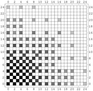
Figure 1: Density plot illustrating the spinor–vector duality in the space of $Z_{2}\times Z_{2}$ heterotic–string vacua. The plot shows the number of models with a given number of $({\bf 16}+\overline{\bf 16})$ and 10 representations of $SO(10)$ and is invariant under exchange of rows and columns, reflecting the spinor–vector duality underlying the entire space of vacua.

Another seminal result from the free fermionic classification program is the discovery of exophobic string vacua [6]. Heterotic–string vacua in which the $SO(10)$ symmetry is broken to a subgroup, while maintaining the $SO(10)$ embedding of the weak hypercharge, necessarily give rise to states in the spectrum that do not satisfy the $SO(10)$ charge quantisation conditions. Some of these states may carry fractional electric charge, which is highly constrained by experiments. However, the exotic states may be confined to the massive spectrum, and not arise as massless states. Such vacua are dubbed as exophobic string vacua. As illustrated in figures 3 and 3, three generation exophobic string vacua were found in the space of fermionic $Z_{2}\times Z_{2}$ orbifolds with $SO(6)\times SO(4)$ gauge symmetry but not with $SU(5)\times U(1)$. The two figures demonstrate again the utility of the free fermion classification method in extracting definite properties of the entire space of scanned vacua. Additional results from the random classification method include the derivation of a string derived extra $Z^{\prime}$ model [19], and string derived $SU(6)\times SU(2)$ GUT model [20].

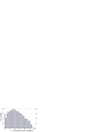
Figure 2: Number of 3–generation models versus total number of exotic multiplets in $SO(6)\times SO(4)$ models.

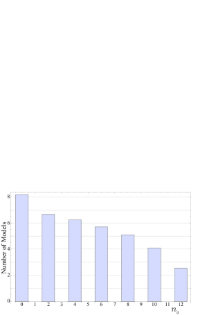
Figure 3: Number of exophobic models versus number of generations in $SU(5)\times U(1)$ models.

5 What do we need machine learning for?

As elaborated in section 4 the free fermionic classification method provides a powerful tool to extract definite properties and results from the space of $Z_{2}\times Z_{2}$ heterotic–string orbifolds. In this section we would like to illustrate how the random classification method reaches the limit of its utility. It demonstrates the need for the application of novel computer methods in the classification program. The limitation of the random search method is apparent when considering the classification of the vacua with $SU(3)\times SU(2)\times U(1)^{2}$ (Standard–like Models (SLM)) [8] or $SU(3)\times U(1)\times SU(2)^{2}$ (Left–Right Symmetric (LRS)) [10] $SO(10)$ subgroups. Unlike the $SO(6)\times SO(4)$ and $SU(5)\times U(1)$, both SLM and LRS cases contain two vectors that break the $SO(10)$ symmetry. In the case of SLM models the basis necessarily contains both vectors $v_{13}$ of eq. (3) and $v_{14}$ of eq. (4). The number of independent GGSO phases hence increases from 66 to 78, or $10^{19.8}$ compared to $10^{24.5}$. In the case of the LRS models the single basis vector $v_{13}\equiv\alpha$ in eq. (5) is sufficient to break the $SO(10)$ symmetry to the LRS subgroup. However, the vector $2\alpha$ breaks the $SO(10)$ symmetry as well. The consequence in both cases is the proliferation of sectors that break the $SO(10)$ symmetry and give rise to exotic states. Table 1 shows the results of a random scan in a space of $10^{11}$ SLM heterotic–string vacua, where heavy Higgs states are those required to break the extra $U(1)$ symmetry embedded in $SO(10)$, to the Standard Model weak hypercharge. Here we note a distinction with respect to the SLM models using the “old school” method. To break the extra $U(1)$ along supersymmetric flat directions at high scale requires the existence in the spectrum of the string SLM the SM singlet state in the 16 representation of $SO(10)$, and its complex conjugate. The “old school” SLM models do not give rise to the complex conjugate state [7]. The “old school” SLMs give rise to exotic Standard Model singlets with 1/2 $U(1)_{Z^{\prime}}$ charge, which are used to break the $U(1)_{Z^{\prime}}$ symmetry along flat directions. As seen from table 1 models containing the standard heavy Higgs states are also not obtained in the random search approach. Moreover, models with light Higgs are not found either. The difficulty stems from the fact that the frequency of three generation models with viable Higgs spectrum is highly diminished.

	Constraints	Total models in sample
	No Constraints	$100000000000$
(1)	+ Three Generations	$28878$
(2)	+ SLM Heavy Higgs	$0$
(3)	+ SLM Light Higgs	$0$
(4)	+ SLM Heavy & Light Higgs	$0$

Table 1: Number of SLM models with phenomenological constraints for sample of $10^{11}$ models.

In table 2 we display similar data in the case of LRS models. The results again illustrate the relative scarcity of viable models in the total sample of vacua. In the case of LRS models we find a three generation model with viable Higgs spectrum at a frequency of 3/$10^{10}$. These results demonstrate the limitation of the random search method for extracting phenomenologically viable models from the total space.

	Constraints	Total models in sample
	No Constraints	$100000000000$
(1)	+ Three Generations	$89260$
(2)	+ LRS Heavy & Light Higgs	$29$

Table 2: Number of LRS models with phenomenological constraints for sample of $10^{11}$ models.

6 Towards machine learning

To remedy the situation a new strategy is required. One possible approach is the genetic algorithm approach developed in [21]. However, while this approach is efficient in extracting phenomenologically viable models, the insight into the structure underlying the larger space of vacua is lost, as it does not provide a classification algorithm. Hence, global properties, like the spinor–vector duality cannot be gleaned in this approach. Consequently a new strategy is required. The basic principle of the new strategy is to reduce the total number of vacua in the space which is being scanned by identifying some condition on the GGSO phases that are amenable for extracting phenomenologically viable vacua.

In the case of the SLMs fertility conditions are identified at the $SO(10)$ level, i.e. involving phases in the $12\times 12$ sub–matrix of the total $14\times 14$ complete matrix of the Standard–like models [7]. These fertility constraints reduce the total number of independent phases to 44. At the $SO(10)$ level we perform a random search. As each $SO(10)$ breaking stage reduces the number of generations by a factor of two, we require $SO(10)$ models with at least twelve generations. Each one of the extracted $SO(10)$ models is now amenable to produce three generation SLMs. We refer to these phase configurations as fertile cores. Around each of these fertile cores we now perform a complete classification of the remaining GGSO phases involving the $SO(10)$ breaking vectors $\alpha$ and $\beta$. Using this methodology generates some $10^{7}$ SLMs, including new Standard–like Models with novel features that were not obtained in the “old school” trial and error method, including models with additional vector–like $Q$ and $\overline{Q}$ and $N$ and $\overline{N}$ states. Adaptation of similar fertility like conditions in the case of the LRS classification is currently underway [22].

7 Conclusions

The $Z_{2}\times Z_{2}$ orbifold provide a case study how string theory may relate to the Standard Model particle data. Early constructions consisted of isolated examples of three generation models, whereas the more modern random classification method yielded of the order of $10^{7}$ viable three generation models with differing $SO(10)$ subgroups. In addition to producing viable three generation models for phenomenological investigations, the classification method provided penetrating insight into the global properties of the space of $(2,0)$ heterotic–string compactification, via e.g. the observation of spinor-vector duality. However, the random method has reached the limit of its usefulness, as seen in the case of the SLMs and LRS models. The case is therefore made for adopting novel computer methods, such as reinforced learning into the classification program, with the basic question at hand whether a computer code can identify the fertility conditions that are amenable for phenomenological considerations.

Acknowledgments

AEF would like to thank the Weizmann Institute, Tel Aviv University, and Sorbonne University for hospitality.

References

References

-
[1]
Antoniadis I, Bachas C and Kounnas C 1987 Nucl. Phys. B289 87;
Kawai H, Lewellen D C and Tye S H H 1987 Nucl. Phys. B288 1. -
[2]
Faraggi A E 1994 Phys. Lett. B326 62; 2002 Phys. Lett. B544 207;
Kiritsis E and Kounnas C 1997 Nucl. Phys. B503 117;
Faraggi A E Forste S and Timirgaziu C 2006 JHEP 0608 57;
Donagi R and Wendland K (2009) J. Geom. Phys. 59 942;
Athanasopoulos P, Faraggi A E, Groot Nibbelink S and Mehta V M 2016 JHEP 1604 38. - [3] Antoniadis I, Ellis J, Hagelin J and Nanopolous D V 1989 Phys. Lett. B231 65.
- [4] Faraggi A E, Rizos J and Sonmez H 2014 Nucl. Phys. B886 202.
- [5] Antoniadis I, Rizos J and Leontaris G 1990 Phys. Lett. B245 161.
- [6] Assel B et al 2010 Phys. Lett. B683 306; 2011 Nucl. Phys. B844 365.
-
[7]
Faraggi A E, Nanopoulos D V and Yuan K, 1990 Nucl. Phys. B335 347;
Faraggi A E 1992 Phys. Lett. B278 131; 1992 Nucl. Phys. B387 239;
Cleaver G B, Faraggi A E and Nanopoulos D V 1999 Phys. Lett. B455 135;
Faraggi A E, Manno E and Timiraziu C 2007 Eur. Phys. Jour. C50 701. - [8] Faraggi A E, Rizos J and Sonmez H 2018 Nucl. Phys. B927 1.
- [9] Cleaver G, Clements D and Faraggi A E 2001 Phys. Rev. D63 066001.
- [10] Faraggi A E, Harries G and Rizos J 2018 Nucl. Phys. B936 472.
-
[11]
Cleaver G, Faraggi A E and Nooij S 2003 Nucl. Phys. B672 64;
Faraggi A E and Sonmez H 2015 Phys. Rev. D91 066006. - [12] Faraggi A E, Kounnas C, Nooij S E M and Rizos J 2004 Nucl. Phys. B695 41.
-
[13]
Faraggi A E and Nanopoulos D V 1993 Phys. Rev. D48 3288;
Faraggi A E 1999 Int. J. Mod. Phys. A14 1663. - [14] For review and references see e.g.: Faraggi A E Galaxies (2014) 2 223.
- [15] For a comprehensive review see e.g.: Ibanez L E and Uranga A M, String theory and particle physics: An introduction to string phenomenology, Cambridge University Press 2012.
- [16] Gregori A, Kounnas C and Rizos J 1999 Nucl. Phys. B549 16.
-
[17]
Faraggi A E, Kounnas C and Rizos J 2007 Phys. Lett. B648 84;
2007 Nucl. Phys. B774 208;
Angelantonj C, Faraggi A E and Tsulaia M 2010 JHEP 1007 004;
Faraggi A E, Florakis I, Mohaupt T and Tsulaia M 2011 Nucl. Phys. B848 332;
Athanasopoulos P, Faraggi A E and Gepner D 2014 Phys. Lett. B735 357. -
[18]
Christodoulides K, Faraggi A E and Rizos J 2011 Phys. Lett. B702 81;
Rizos J 2014 Eur. Phys. Jour. C74 010. - [19] Faraggi A E and Rizos J 2015 Nucl. Phys. B895 233.
- [20] Bernard L et al 2013 Nucl. Phys. B868 1.
- [21] Abel S and Rizos J 2014 JHEP 1408 010.
- [22] Faraggi A E, Harries G, Percival B and Rizos J, paper in preparation.