Spin polarization and orbital effects in superconductor-ferromagnet structures
Abstract
We study theoretically spontaneous currents and magnetic field induced in a superconductor-ferromagnet (S-F) bilayer due to direct and inverse proximity effects. The induced currents are Meissner currents that appear even in the absence of an external magnetic field due to the magnetic moment in the ferromagnet and to the magnetization in the superconductor . The latter is induced by the inverse proximity effect over a distance of the order of the superconducting correlation length . On the other hand the magnetic induction , caused by Meissner currents, penetrates the S film over the London length . Even though usually exceeds considerably the correlation length, the amplitude and sign of at distances much larger than depends crucially on the strength of the exchange energy in the ferromagnet and on the magnetic moment induced in the in the S layer.
I Introduction
Besides the orbital effects, it is well known that conventional superconducting pairing is also suppressed by a magnetic field when acting on the spins of electrons via the Zeeman interaction. Whereas superconducting correlations couple pairs of electrons in a singlet state (Cooper pairs), the Zeeman interaction tends to align both spins in the direction parallel to the magnetic field. These two antagonistic tendencies can nevertheless coexist when the Zeeman energy is small enough in comparison to the superconducting gap. This coexistence implies the appearance of Cooper pairs in a triplet state. This situation occurs, for example, in thin superconducting films (S films) in the presence of an in-plane magnetic field, and also in superconductor-ferromagnet (S-F) heterostructure in which Cooper pairs from the S layer can penetrate into the ferromagnet where the intrinsic exchange field of the F acts on the spins of electrons (see review articles GolubovRMP04 ; BuzdinRev05 ; BVErev05 ; EschrigRev11 ; LinderRev15 ; LinderBalRev17 ).
Leakage of Cooper pairs from S to F is the so called proximity effect. The wave function of the Cooper pairs penetrating into the F region with a uniform magnetic moment contains not only the singlet but also the triplet component with zero spin projection onto the vector . At the same time, provided the S-F interface is transparent enough, these triplet pairs can leak into the superconductor, inverse proximity effect, and a finite magnetic moment in S appearsBVE04 ; BVEepl04 ; footnoteM .
The size of this spin-polarized region within the superconductor is of the order of the superconducting correlation length, which in the diffusive limit is given by . The magnetic moment induced in S, has a direction opposite to the magnetization vector in the F layer. Under certain conditions the total magnetic moment in the S region compensates the total magnetic moment of the F film resulting in a full spin screeningBVE04 ; BVEepl04 ; foot In the ballistic case, the induced magnetization may spatially change sign Bergeret05 ; Kharitonov06 .
These predictions for the inverse proximity effect have eventually been confirmed experimentally Garifullin09 ; Kapitulnik09 . However, quantitative interpretation of the experimental results is quite subtlediBernardo ; Flokstra , since the magnetic field arising in S is caused not only by the induced magnetization but also by Meissner currents that arise in the S/F structurePRB01 ; BVEepl04 ; Buzdin18 . For this reason a detailed understanding of the inverse proximity effect is a key issue for interpretation of experimental data on S/F structures.
In this work we study the proximity effect in S-F structures taking into account explicitly the generated spontaneous currents. This topic was first addressed by the authors in 2004 BVEepl04 and more recently in Ref. Buzdin18 . These two works predict a magnetic induction induced in the S layer which penetrates over the London penetration depth . The authors of Ref.BVEepl04 focus on the magnetic field caused by and estimated the orbital effects. They showed that the spin polarization effects are stronger than those related to the Meissner currents screening the magnetic moment . In Ref.Buzdin18 the orbital effects were studied in more detail, but the inverse proximity effect was completely neglected. Since in dirty superconducting films is usually larger than the coherence length characterizing penetration of a magnetic moment into S, it might look at first glance as if the magnetic field measured in a superconducting film with a large thickness (), could not be affected by the magnetic moment localized close to the S-F interface. In contrast to this scenario, we demonstrate here that for a correct interpretation of the experimental data one does need to take into account the magnetic moment in the S layer induced by the inverse proximity effect.
To be specific, we show that the spatial dependence of the magnetic induction induced in the S region consists of a long-range component which decreases over the London penetration depth , and of a short-range component caused by the induced magnetization which decays over the superconducting coherence length . The magnetic inductance, , in a thick superconducting film () has thus the form:
| (1) |
At large distances from the S/F interface, , is mainly determined by the long-range term . Its amplitude consists of two contributions:
| (2) |
The first term is the contribution from the spontaneous Meissner currents (orbital effects) and equals
| (3) |
where , and are the thickness of the F layer and the London penetration depth in the ferromagnet, respectively. This expression coincides with the result for the magnetic induction obtained in Ref. Buzdin18 . One of our main findings below, is that there is an additional contribution to the magnetic induction, the term in Eq. (2). This contribution is caused by the inverse proximity effect it was neglected in Ref. Buzdin18 . For a wide range of parameters this contribution due to spin polarization near the S/F interface is much larger than that due to orbital effects, i.e. . Moreover, this contribution might be crucial in determining the sign of the magnetic induction in the S layer since, as we show below, and have different signs. Moreover, the relative magnitude between these two contributions depends on the exchange field in the F layer. The contribution due to spin polarization in S can be neglected only in case of F film with sufficiently large exchange energy .
In the next sections we investigate the spatial distribution of the Meissner currents and the fields , . Our main findings are the following: (i) Eq.(3) describes the orbital effect only in the case of rather large exchange energy . However, in this case the induced field is small since the inverse London penetration depth is small; (ii) In the full screening case, both short- and long-range components in Eq.(2) are determined by spin polarization effects; (iii) Meissner currents in the S region change sign at some point away from the S/F interface; (iv) the total Meissner currents in the F (or S) film calculated with or without account for the spin screening effect may have opposite directions, and (v) in the case of an out-of-plane magnetization of the F layer no spontaneous currents, and hence no magnetic induction, are induced.
The article is organized as follows. In the next section we consider a diffusive S/F bilayer and derive the expressions for the magnetic moment induced by the spin polarization. Although this have been presented in our earlier publications BVE04 ; BVEepl04 , for completeness and to set the notation, we re-derive it here. In section III we solve the magnetostatic equations for the vector potential and find the spatial distribution of the spontaneous supercurrents in the system which arise in the absence of an external magnetic field. In particular we show that the current density in the S film can change its sign near the S/F interface. In the last section we summarize our results.
II Proximity effect in S-F Heterostructure
In this section we study the proximity effect in an S-F strcuture. We assume the diffusive limit, such that the conditions and are satisfied, where is the momentum relaxation time. The presence of a spin-dependent term in the F region means that the condensate induced in this layer consists of a singlet and triplet component. In turn, triplet Cooper pairs may penetrate into the S region and induce a finite spin polarization. To describe this processes in a diffusive system, we use the quasiclassical Green’s functions (GF) Kopnin ; Footnote1 and the generalized Usadel equation BVErev05 ; BSVH2018 .
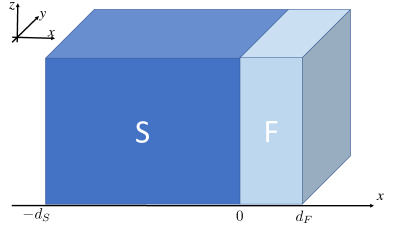
Specifically, we consider the structure shown in Fig. 1. It consists of a ferromagnetic layer of thickness and a superconducting layer of thickness . In the absence of proximity effect the Green function in S corresponds to the the bulk BCS matrix Green function which has the form
| (4) |
where are the Pauli matrices operating in the particle-hole space and , Here is the fermionic Matsubara frequency.
In the presence of an exchange field , the quasiclassical Green’s function maintains its structure in the particle-hole space but its components are matrices in the spin-space. We consider here only a mono-domain ferromagnet with an homogenous and therefore the general form of in S and F is
| (5) |
where is the third Pauli matrix in the spin space, and the index means . In Eq.(5) the terms proportional to are the normal Green funcions (GF)which determine the electronic charge and spin densities. The terms proportional to are the anomalous GF describing the singlet and zero-spin projection triplet components of the condensate. Without losing generality we assume that the exchange field points in -direction, .
The GFs can be calculated by solving the Usadel equation complemented with proper boundary conditions (see Appendix A for detail). The GF calculated in this way determine the current and electron magnetization density, as follows
| (6) |
| (7) |
here and are an effective Bohr magneton and the normal density of states at the Fermi level respectively. is the magnetization in the normal state which is finite, and spatially homogeneous, only in the F layer.
Clearly the matrix defined in Eq.(5) is diagonal in the spin space. This simplifies the calculation of since the equations for up and down spins decouple from each other. In other words, one can write the GF as and solve the problem independently for spins. Qualitatively, due to conventional proximity effect, a spin dependent condensate function is induced in the F layer. Such spin-polarized condensate can penetrate back into the S region inducing a local magnetic moment described by the corrections to the GF defined as . All these functions can be obtained from the Usadel equation, as explained in Appendix A.
In order to solve the problem analytically we assume that the F film is thin enough , , and therefore the matrix can be considered almost constant in space. We also assume that the S-F interface has a finite interface resistance per unit area, . This allows us to use the Kupriyanov-Lukichev boundary condition (46). Then we can integrate spaatially the Usadel equation, Eq. (44), in the F region to obtain following algebraic equation for :
| (8) |
where , , , and is the conductivity of the F layer. Equation (8) has to be solved together with the normalisation condition . The solution has the same structure as the bulk BCS solution with renormalized and . cf. Eq, (4)
| (9) |
where .
On the superconducting side of the interface, the GF are modified due to the inverse proximity effect. Provided the transmission of the S/F interface is finite, a correction to the BCS Green’s functions arises in the S film. We assume that the elements of the matrix are small̇: . Then, in the leading order approximation we obtain and So, the magnetisation density induced in the S film is given by
where , and The function is defined in Eq. (5) and explicitly given in the appendix Eq.(51). The total magnetic moment induced in the superconductor is obtained by integrating the previous expression in the interval
| (11) |
| (12) |
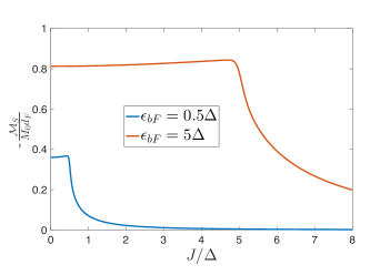
where the functions and are defined in Eqs.(4,9). In Fig. 2 we represent the dependence of the normalized total magnetic moment in the S region on the exchange energy for two values of : and . One can clearly see a kink at . When , the characteristic energy describes the subgap induced in the F film due to proximit effect. In this case the induced magnetization is small and there is no full screening. In contrast, in the limit an almost full screening takes place provided
One can analytically calculate the total magnetisation in the superconducting region in the limit . This condition combined with Eq.(52) can be written as
| (13) | |||||
| (14) |
In this limit one obtains and , where . The term () in Eq.(11) is approximately equal to
| (15) |
where is the magnetic moment in F in the absence of the proximity effect, and we used the relation . At low temperatures , the summation in Eq.(11) is transformed into integration over that givesBVEepl04
| (16) |
This means that in the limiting case considered here the total magnetic moment of Cooper pairs induced in the S region compensates the magnetic moment of the F filmfootnoteM If the condition (13) is not fulfilled or the temperature is not low enough the screening is not complete and . In the other limiting case of a large exchange field the induced magnetic moment in S is given by
| (17) |
and therefore the screening is very weak.
The magnetic moment induced right of the S-F interface can be calculated from Eq.(15) in the limit of low temperatures when the function is approximated
| (18) |
with . We then obtain
| (19) |
with .
The magnetization in the F film can be written in the form , where is the uniform magnetization of the ferromagnet in the absence of the proximity effect and is a correction due to the proximity effect. As we consider a thin F layer with , the correction can be assumed constant in space. It can be shown that is negative, which leads to a decrease of the magnetization of the F filmBVE04 . However, in what follows we neglect since it does not affect qualitatively the main results.
We note that the condition, Eq. (13), can be fulfilled in experiments with weak ferromagnets, as for example in Nb/CuNi structures as those used in Ref.RyazanovPRL06 . By taking , , and , we obtain and . For these parameters the condition in Eq.(13) is satisfied provided the energy is not too large
In this section we analyzed the proximity effect on the magnetic moment induced in S. In the next section we find the spatial distribution of the Meissner currents and magnetic fields in the whole S-F bilayer.
III
Magnetostatics of a S-F bilayer
In this section we determine the currents and fields induced in the S/F structure shown in Fig. 1. The total current consists of two contributions: the Meissner contribution and the current stemming from the finite magnetization in the system. The magnetic induction and the magnetic field obey the Maxwell equation both in the F and S films
| (20) | |||||
| (21) |
where is the Meissner current denoted as in S or F films, respectively. In the F film, the current is carried by Cooper pairs induced due to the proximity effect. Both currents are related to the vector potential via the London equation:
| (22) |
where is the London penetration length. We neglect variation of due to the proximity effect and assume that it is constant. Moreover, in case of superconducting films with a short mean free path the coherence length is usually much smaller than , which is equivalent to the limit of a large Ginzburg-Landau parameter ,
| (23) |
where , and are the the concentration of free carriers, effective mass and mean free path, respectively. For typical values of and one obtains as upper limit for the mean free path is .
In what follows we solve Eq.(24) for two different cases: in-plane and out-of-plane orientation of .
III.1 In-plane magnetization
In this case and and . This menas that and . Then, Eq. (24) reduces to
| (25) |
As mentioned above, in the thin F film the magnetization is assumed to be almost constant and therefore one can neglect the r.h.s of the previous equation in the F region. The solution of Eq. (25) in the F layer within the limit can be written as
| (26) |
where the coefficients and are integration constants.
Whereas in the S region the equation for is obtained by using Eq. (II) for the induced in S:
| (27) |
As demonstrated in the previous section the induced magnetization (right-hand side of Eq. 27) decays on a length of the order . Since we consider the case , the solution in the superconductor can be written as
| (28) |
where is a third integration constant, is a small parameter (see Eq.(23)), and . From Eq. (28), one can obtain the expressions for and , as shown in Appendix B.
The integration constants , , and in Eqs.(26, 28) are determined by the following boundary conditions
| (29) |
where . The first and second equations provide the continuity of the vector potential and the field at the interface. The condition assumes the presence of an external magnetic field but in what follows we assume that .
In the main approximation we find three coupled equations determining , and . Their solution is given by
| (30) | |||||
| (31) | |||||
| (32) |
where , , and . In deriving these equations we have used expression Eq. (11) for the total magnetisation induced in the S region.
Before analyzing the full spatial solution of the boundary problem let us focus on the value of vector potential at the outer interface, . The expression can be straightforwardly obtained from the above equation and reads:
| (33) |
From this expression one can already draw important conclusions regarding the vector potential and supercurrents, at large distances from the boundary. Let us consider two cases:
Case a): If one neglects the inverse proximity effect as done in Ref. Buzdin18 , the first and third term in the numerator of Eq. (33) are zero and one obtains ()
| (34) |
The corresponding magnetic induction at large distances from the S/F interface coincides with Eq. (3)
Case b): If one takes into account the inverse proximity effect then the second contribution anticipated in Eq. (2) appears. Specifically in the full screening situation (), one obtains
| (35) |
where and .
Clearly these two limiting cases describe very different situations, in which the spontaneous currents have even different signs. It is important to emphasize that even though the magnetization induced in the S layer occurs over the coherence length , it changes drastically the vector potential at distances of the order of .
From the knowledge of the vector potential one can write the current density using the London equation, Eq.(22), as . The total currents through the F and S layers is then defined as
| (36) |
From Eqs.(26,28) and in the leading order in our approach we find that
| (37) |
and
| (38) |
As there is no external field the currents sums to zero, . Remarkably, in the two limiting cases, a) and b), the total current in the S and F films has a different sign, i.e. .
Ff is large enough there is a transition from positive to negative determined by a critical . Indeed, we obtain from Eqs.(17)
| (39) |
with .
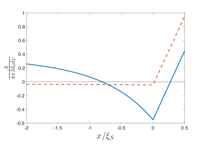
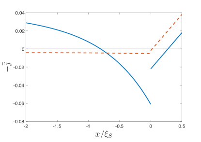
In Fig. 3 we compare the spatial dependence of (upper panel) and of the current density induced in the system (lower panel), in the two cases, a) no spin polarisation; , and b) when the inverse proximity effect is taken into account. One clearly sees qualitative differences between these two cases. In case b) the spontaneous currents change sign at certain distance from the interface of the order of , whereas in case a) the sign of the current in S is constant. In addition, the amplitude of the spontaneous currents, and hence of the magnetic inductance Eq. (2), generated far from the S/F interface is much larger in case b). These results demonstrate that for a correct interpretation of experiments the induced magnetization in the superconductor cannot be simply neglected.
III.2 Out-of-plane magnetization
Finally in this section we consider the case of a F layer with out-of-plane magnetization: . The field with is determined from the equation :
| (40) |
Thus we obtain
| (41) |
Equation then yields
| (42) |
The magnetic induction , does not depend on and equals zero both in the S and F films.
IV Conclusions
We have studied the spatial dependence of the Meissner currents and magnetic induction that spontaneously arise in an S/F structure even in the absence of an external field . The fields and originate due to the orbital and spin polarization effects and contain long-range and short-range components (see Eq.(1)). The amplitude of the short-range component is due to the inverse proximity effect and is much larger than . On the other hand, the amplitude of the long-range component is caused by both, the Meissner currents and the spin polarization, and depends on the magnitude of the exchange energy in the F film. It changes sign at being negative for and positive for . Note that at large the field and are small because both spin polarization (see Eq.(17)) and orbital effects are small. In Ref. Buzdin18 the inverse proximit effect was neglected and therefore only the orbital contribution was obtained, where . However, as explained above, by decreasing the exchange energy , the inverse proximity effect prevails, leads to a finite magnetic moment , and to a change of sign of changes sign. In such a case its magnitude clearly exceeds the value of . Moreover, also the results for the vector potential , and hence for the current density , depend crucially on the inverse proximity effect (case (b) in section III.1) and are qualitatively different to the case in which this effect is neglected (case (a) in section III.1 and Ref. Buzdin18 ). In particular, we find that the Meissner current density changes sign in the S region if the induced magnetization is taken into account.
Acknowledgements
F.S.B acknowledges financial support from Horizon research and innovation programme under grant agreement No. 800923 (SUPERTED) the Spanish Ministerio de Economía, Industria y Competitividad (MINEICO) under Project FIS2017-82804-P.
Appendix A Solution of the Usadel equation in the S-F strcuture
The Usadel equations have the form
| (43) |
| (45) |
and the boundary conditions (KupLukichev88 )
| (46) |
where -1, is the interface resistance per unit area.
| (48) |
which follows from the normalization condition, Eq.(45).
The induced magnetization is determined by the component Tr (see Eq.(6)). We multiply Eq.(47) by and calculate the trace. We find the solution
| (49) |
The integration constant is found from the boundary condition Eq.(46) that yields
| (50) |
where Im and Im. The function is defined in Eq.(9).
We obtain for
| (51) |
One can see that this correction is small if the condition
| (52) |
is fulfilled, that is, .
Appendix B The magnetic field
For completeness we show in this appendix the expressions for the magnetic induction and magnetic field which can be obtained from Eqs.(26,28)
| (53) | |||||
| (54) |
| (55) | |||||
| (56) |
where .
References
- (1) A. A. Golubov, M. Yu. Kupriyanov, and E. Il’ichev, Rev. Mod. Phys. 76, 411 (2004)
- (2) A. I. Buzdin, Rev. Mod. Phys. 77, 935 (2005).
- (3) F. S. Bergeret, A. F. Volkov, and K. B. Efetov, Rev. Mod. Phys. 77, 1321 (2005).
- (4) M. Eschrig, Phys. Today 64(1), 43 (2011); Rep. Prog. Phys. 78, 104501 (2015).
- (5) J. Linder and J. W. A. Robinson, Nature Physics 11, 307-315 (2015).
- (6) Odd-frequency superconductivity, J. Linder, A. V. Balatsky, arXiv:1709.03986.
- (7) B. S. Chandrasekhar, Appl. Phys. Lett. 1, 7 (1962).
- (8) A. M. Clogston, Phys. Rev. Lett. 9, 266 (1962).
- (9) F. S. Bergeret, A. F. Volkov, and K. B. Efetov, Phys. Rev. Lett. 86, 3140 (2001).
- (10) M. Eschrig, J. Kopu, J. C. Cuevas, and G. Schon, Phys. Rev. Lett. 90, 137003 (2003).
- (11) L. P. Gor’kov and A. I. Rusinov, JETP 46, 1363 (1964), Sov. Phys. JETP 19, 922 (1964).
- (12) P. Fulde and R. A. Ferrell, Phys. Rev. 135, A550 (1964).
- (13) A. J. Larkin and Y. N. Ovchinnikov, Zh. Eksp. Teor. Fiz. 47, 1136 (1964); Sov. Phys. JETP 20, 762 (1965).
- (14) L. N. Bulaevskii, V. V. Kuzii, and A. A. Sobyanin, , Pis’ma Zh. Eksp. Teor. Fiz. 25, 314 (1977); JETP Lett. 25, 290–294 1977 .
- (15) A. I. Buzdin and M. Y. Kuprianov, Pis’ma Zh. Eksp. Teor. Fiz. 53, 308 (1991) [JETP Lett. 53, 321 (1991)].
- (16) V. V. Ryazanov, , V. A. Oboznov, A. Yu. Rusanov, A. V. Veretennikov, A. A. Golubov, and J. Aarts, Phys. Rev. Lett. 86, 2427 (2001).
- (17) V. A. Oboznov, V. V. Bol’ginov, A. K. Feofanov, V. V. Ryazanov, and A. I. Buzdin, Phys. Rev. Lett. 96, 197003 (2006)
- (18) H. Sellier, C. Baraduc, F. Lefloch, and R. Calemczuk, Phys. Rev. B 68, 054531 (2003).
- (19) T. Kontos, M. Aprili, J. Lesueur, F.Genet, B. Stephanidis, and R. Boursier, Phys. Rev. Lett. 89, 137007 (2002).
- (20) M. Weides, M. Kemmler, E. Goldobin, D. Koelle, R. Kleiner, H. Kohlstedt, and A. Buzdin, Appl. Phys. Lett. 89, 122511 (2006).
- (21) R. S. Keizer, S. T. B. Goennenwein, T. M. Klapwijk, G. Miao, G. Xiao, and A. Gupta, Nature 439, 825 (2006).
- (22) I. Sosnin, H. Cho, V. T. Petrashov, and A. F. Volkov, Phys. Rev. Lett. 96, 157002 (2006).
- (23) M. S. Anwar, F. Czeschka, M. Hesselberth, M. Porcu, and J. Aarts, Phys. Rev. B 82, 100501 (2010); M. S. Anwar and J. Aarts, Supercond. Sci. Technol. 24, 024016 (2011); M. S. Anwar, M. Veldhorst, A. Brinkman, and J. Aarts, Appl. Phys. Lett. 100, 052602 (2012).
- (24) T. S.Khaire, M. A. Khasawneh, W. P. Pratt, Jr., and N. O. Birge, Phys. Rev. Lett. 104, 137002 (2010); C. Klose, T. S. Khaire, Y. Wang, W. P. Pratt, Jr., N. O. Birge, B. J. McMorran, T. P. Ginley, J. A. Borchers, B. J. Kirby, B. B. Maranville, and J. Unguris,Phys. Rev. Lett. 108, 127002 (2012).
- (25) W. M. Martinez, W. P. Pratt, Jr., and N. O. Birge, Phys. Rev. Lett. 116, 077001 (2016).
- (26) D. Sprungmann, K. Westerholt, H. Zabel, M. Weides, and H. Kohlstedt, Phys. Rev. B 82, 060505(R) (2010).
- (27) J. W. A. Robinson, J. D. S. Witt, and M. G. Blamire, Science 329, 59 (2010); J. W. A. Robinson, G. B. Halász, A. I. Buzdin, and M. G. Blamire, Phys. Rev. Lett. 104, 207001 (2010).
- (28) M. G. Blamire and J. W. A. Robinson, J. Phys. Condens. Matter 26, 453201 (2014).
- (29) D. Massarotti, N. Banerjee, R. Caruso, G. Rotoli, M. G. Blamire, and F. Tafuri, Phys. Rev. B 98, 144516 (2018).
- (30) M. S. Kalenkov, A. D. Zaikin, and V. T. Petrashov, Phys. Rev. Lett. 107, 087003 (2011).
- (31) F. S. Bergeret, A. F. Volkov, K. B. Efetov, Phys. Rev. B 64, 134506 (2001)
- (32) F. S. Bergeret, A. F. Volkov, K. B. Efetov, Phys. Rev. B 68, 064513 (2003).
- (33) F. S. Bergeret, A. F. Volkov, K. B. Efetov, Europhys.Lett.66,111(2004).
- (34) F. S. Bergeret, A. Levy Yeyati, A. Martin-Rodero, Phys. Rev. B 72, 064524 (2005).
- (35) M. Yu. Kharitonov, A. F. Volkov, K. B. Efetov, Phys. Rev. B 73, 054511 (2006).
- (36) Here and in the rest of the article, when talking about spin screening, we refer to the screening of the magnetic moment of free electrons (itinerant ferromagnet) which equals to . The contribution to the magnetization of F stemming from localized magnetic moments is not screened by the inverse proximity effectBVE04 .
- (37) T. Tokuyashu, J. A. Sauls and D. Reiner, Phys. Rev. B 38, 8823 (1988)
- (38) V.N. Krivoruchko and E.A. Koshina, Phys. Rev. B 66, 014521 (2002)
- (39) Note that induced magnetisation in S was also considered in a ferromagnetic-insulator/superconductor structure Tokuyashu02 ; Koshina02 . Whereas in Ref. Koshina02 a diffusive S/F bilayer was analysed. Contrary to our results, in the latter work the induced magnetization obtained has the same orientation as the magnetic moment in the ferromagnet.
- (40) R. I. Salikhov, I. A. Garifullin, N. N. Garif’yanov, L. R. Tagirov, K. Theis-Brohl, K. Westerholt, and H. Zabel, Phys. Rev. Lett. 102, 087003 (2009).
- (41) J. Xia, V. Shelukhin, M. Karpovski, A. Kapitulnik, and A. Palevski, Phys. Rev. Lett. 102, 087004 (2009).
- (42) A. Di Bernardo, et al. Phys. Rev. X 5, 041021 (2015).
- (43) M.G. Flokstra et al. Nature Phys. 12, 57 (2016).
- (44) S. Mironov, A. S. Mel’nikov, A. Buzdin, Appl. Phys. Lett. 113, 022902 (2018).
- (45) F. S. Bergeret, M. Silaev, P. Virtanen, T. T. Heikkilä, Rev. Mod. Phys, 90. 041001 (2018).
- (46) C. Huang, I. V. Tokatly, and F. S. Bergeret, Phys. Rev. B 98, 144515 (2018).
- (47) The derivation of formulas for the induced magnetic moments was briefly given in BVE04 ; BVEepl04 . We use here a slightly different structure of the quasiclassical Green’s functions that is moire convenient for our description.(see, for example, MVEChiral16 ; BSVH2018 ). A connection between the most customary basis used in the literature for the Green’s functions has been presented in Ref. Huang2018
- (48) A. Moor, A. F. Volkov, K. B. Efetov, Phys. Rev. B 93, 104525 (2016).
- (49) K.D. Usadel, Phys. Rev. Lett. 25, 507 (1970).
- (50) N. Kopnin, Theory of Nonequilibrium Superconductivity, (Oxford Science, London, 2001).
- (51) M. Yu. Kupriyanov and V. F. Lukichev, Zh. Eksp. Teor. Fiz. 94, 139 (1988) [Sov. Phys. JETP 67, 1163 (1988)]