Generative framework for dimensionality reduction of large scale network of non-linear dynamical systems driven by external input

Abstract

Several studies have proposed constraints under which a low dimensional representation can be derived from large-scale real-world networks exhibiting complex nonlinear dynamics. Typically, these representations are formulated under certain assumptions, such as when solutions converge to attractor states using linear stability analysis or using projections of large-scale dynamical data into a set of lower dimensional modes that are selected heuristically. Here, we propose a generative framework for selection of lower dimensional modes onto which the entire network dynamics can be projected based on the symmetry of the input distribution for a large-scale network driven by external inputs, thus relaxing the heuristic selection of modes made in the earlier reduction approaches. The proposed mode reduction technique is tractable analytically and applied to different kinds of real-world large-scale network scenarios with nodes comprising of a) Van der Pol oscillators b) Hindmarsh-Rose neurons. These two demonstrations elucidate how order parameter is conserved at original and reduced descriptions thus validating our proposition.

Large-scale dynamical systems are useful tools to explain a wide variety of complex phenomena in nature e.g. financial markets HSIEH , jamming transitions Charbonneau et al. (2017), human mobility dynamics Song et al. (2010), weather patterns Antoulas et al. (2010) and brain dynamics Deco et al. (2008). While increase in scale or dimensions may increase the predictive power of the model system, nonetheless a reduction to simpler descriptions at lower dimensions is critical for having relevance to empirical observations and analytical tractability of underlying mechanisms governing empirical observations. One robust approach of reducing dimensions is defining modes on which the original system can be projected Antoulas et al. (2010); Stefanescu and Jirsa (2008). The selection of a mode is often heuristically motivated, and the mode can also be an order parmeter from the perspective of the paradigmatic framework of Synergetics Haken (1983). In Neuroscience, reduction of dynamical systems with respect to modes constructed from distribution of external input has been performed earlier on small-scale network of linearly coupled excitable systems Stefanescu and Jirsa (2008). Since this reduction retain important network dynamics, large-scale networks were conceptualized by coupling these reduced systems with long-range coupling Becker et al. (2015); Sanz-Leon et al. (2015), the later being heuristically argued from symmetry properties. In present work, we perform reduction on a large-scale network where connection among nodes involve global and local coupling mimicking a real-world system. Subsequently, long-range coupling term between modes in the reduced system is derived analytically as part of the reduction process. Global coherence is an order parameter that can be computed both at the level of original dynamical system as well as from the mode dynamics in the reduced system. Conservation of global coherence at both levels is used to validate the generality of our approach in two distinct networks. First, we simulate a large-scale network where each node is a Van der Pol oscilator having 2-dimensional dynamics and coupled using local and global parameters. Second each node is a Hindmarsh-Rose neuron, a 3-dimensional dynamical system which can exhibit different time scales of oscillations resulting in bursting along with tonic spiking behavior.

Each $i^{th}$ excitable system in node $n$ is represented by a vector of state variables (state vector) $\bm{x}^{(n)}_{i}$. Input to $i^{th}$ excitable system from interaction with other excitable systems within $n^{th}$ node is given by a vector function $\bm{g}\left(\{\bm{x}^{(n)}_{j}\},K,i\right)$ where $K$ is coupling constant and $\{\bm{x}^{(n)}_{j}\}$ is a set of $J$ state-vectors ($j=1,...,J$) in $n^{th}$ node. Input to every excitable system in $n^{th}$ node from other nodes is given by another vector function $\bm{h}\left(\{\bm{x}_{j}^{(m)}\},W,n\right)$ where elements of matrix $W$ ($W\in\Re^{J\times N}$) are the weights of connections between nodes and $\{\bm{x}_{j}^{(m)}\}$ is a set of state-vectors in $N$ nodes ($m=1,...,N$) (Figure 1A). Vector function $\bm{f}(\bm{x}_{i}^{(n)})$ contributes to the local dynamics of $i^{th}$ excitable system in $n^{th}$ node. Then, the dynamics of the entire system is described by the following set of equations

$$\tau_{n}\dot{\bm{x}}^{(n)}_{i}= \bm{f}\left(\bm{x}_{i}^{(n)}\right)+\bm{g}\left(\{\bm{x}^{(n)}_{j}\},K,i\right)+$$ (1)

$$\bm{h}\left(\{\bm{x}_{j}^{(m)}\},W,n\right)+\bm{\phi}\left(\bm{I}_{i}^{(n)}\right)$$

where $\dot{\bm{x}}$ is time derivative of state vectors, $\bm{\phi}$ is a function of the external input ($\bm{I}$) and $\tau_{n}$ is the time-constant of $n^{th}$ node which is a differentiating factor between nodes. However, within $n^{th}$ node, external current to $i^{th}$ excitable system ($\bm{I}^{(n)}_{i}$) differentiates it from the rest. For a large scale network comprising of individual excitable nodes, (1) can be written as

$$\tau_{n}\dot{\bm{x}}^{(n)}(t,\bm{I})= \bm{f}\left(\bm{x}^{(n)}\right)+\bm{g}\left(\bm{x}^{(n)},K\right)+$$ (2)

$$\bm{h}\left(\{\bm{x}^{(m)}\},W,n,i\right)+\bm{\phi}\left(\bm{I}\right)$$

where $I$ is a continuous variable having normal distribution $\mathbb{N}(\mu,\sigma)$.

Now, we can represent $\bm{x}(t,I)$ as a superposition of $M$ bi-orthogonal modes $\{v_{i}\}$

$$\bm{x}(t,\bm{I})=\sum_{i=1}^{M}\bm{\xi}_{i}(t)v_{i}(\bm{I})+R(t,\bm{I})$$ (3)

where $R(t,\bm{I})$ is the residual and $M\lll J$ (Figure 1B). The nature of reduction is such that dynamical system given in (1) is reduced to solving for the mode coefficients $\bm{\xi}_{i}$ as described in the following set of equations

$$\tau_{n}\dot{\bm{\xi}}^{(n)}_{i}= \bm{F}\left(\bm{\xi}_{i}^{(n)}\right)+\bm{G}\left(\{\bm{\xi}^{(n)}_{j}\},K,i\right)+$$ (4)

$$\bm{H}\left(\{\bm{\xi}_{j}^{(m)}\},W,n,i\right)+\bm{II}_{i}^{(n)}$$

where

$$\bm{\xi}_{i}= \int_{I}\bm{x}(t,I)v^{+}_{i}dI$$

$$\bm{F}\left(\bm{\xi}_{i}\right)= \int_{I}\bm{f}\left(\bm{x}\right)v_{i}^{+}dI$$

$$\bm{G}\left(\{\bm{\xi}_{j}\},K,i\right)= \int_{I}\bm{g}\left(\bm{x},K\right)v_{i}^{+}dI$$

$$\bm{H}\left(\{\bm{\xi}^{(m)}_{j}\},W,n,i\right)= \int_{I}\bm{h}\left(\{\bm{x}^{(m)}\},W,n,i\right)v_{i}^{+}dI$$

$$\bm{II}_{i}^{(n)}= \int_{I}\bm{I}v_{i}^{+}dI$$

and $\{v_{i}^{+}\}$ are the adjoint basis for the biorthogonal modes $\{v_{i}\}$.

Large-scale network of Van der Pol oscillators:

A Van der Pol oscillator van der Pol (1920) has two state variables $x$ and $y$ which follows the following equations

$$\dot{x}= y$$

$$\dot{y}= -a(x^{2}-1)y-x$$ (5)

A large-scale network where individual node is essentially a Van der Pol oscillator can be cast into equation (1) with the following relations

$$\bm{f}\left(\bm{x}_{i}\right)= \left[\begin{array}[]{c}y_{i}\\ -a({x_{i}}^{2}-1)y_{i}-x_{i}\end{array}\right]$$ (8)

$$\bm{g}\left(\{\bm{x}_{j}\},K,i\right)= \left[\begin{array}[]{c}K(\mathbb{E}[\{x_{j}\}]-x_{i})\\ 0\end{array}\right]$$ (11)

$$\bm{h}\left(\{\bm{x}_{j}^{(m)}\},W,n\right)= \left[\begin{array}[]{c}\sum_{m=1}^{N}W_{nm}\mathbb{E}[\{x^{(m)}_{j}\}]\\ 0\end{array}\right]$$ (14)

$$\bm{I}= \left[\begin{array}[]{c}I\\ 0\end{array}\right]$$ (17)

where $a$ is a constant and $\mathbb{E}[\{x_{j}\}]$ is the expected value of the state-variables $\{x_{j}\}$. For the reduced system described in (4) with $\xi_{i}=[\alpha_{i},\beta_{i}]^{T}$, we derive

$$\bm{F}\left(\bm{\alpha}_{i}\right)= \left[\begin{array}[]{c}\beta_{i}\\ -a_{i}{\alpha_{i}}^{2}\beta_{i}+a\beta_{i}-\alpha_{i}\end{array}\right]$$ (20)

$$\bm{G}\left(\{\bm{\alpha}_{j}\},K,i\right)= \left[\begin{array}[]{c}K\left(\sum_{j=1}^{M}A_{ij}\alpha_{j}-\alpha_{i}\right)\\ 0\end{array}\right]$$ (23)

$$\bm{H}\left(\{\bm{\alpha}^{(m)}_{j}\},W,n,i\right)= \left[\begin{array}[]{c}\sum_{m=1}^{N}W_{nm}\sum_{j=1}^{M}A_{ij}\alpha^{(m)}_{j}\\ 0\end{array}\right]$$ (26)

$$\bm{II}= \left[\begin{array}[]{c}II\\ 0\end{array}\right]$$ (29)

where the constants $a_{i}$ and $A_{ij}$ are computed by applying bi-orthogonal assumption of modes as stated in Appendix A.

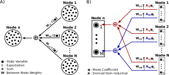
Figure 1: A) Large-scale network architecture of complete system where input to a node is the weighted sum of expected value of state-variables B) Large-scale network architecture of proposed reduced system where input to a target-mode is weighted sum of target-mode specific expected mode activity from other nodes.

Large-scale network of Hindmarsh-Rose neurons:

In Neuroscience, Hindmarsh-Rose (HMR) neuron is a three dimensional model of single neuron firing dynamics having three state variables Hindmarsh and Rose (1984)

$$\dot{x}= y-ax^{3}+bx^{2}+I-z$$

$$\dot{y}= c-dx^{2}-y$$

$$\dot{z}= r(s(x-x0)-z)$$ (30)

where $a$, $b$, $c$, $d$, $r$, $s$ and $x0$ are the constants. A network of excitatory and inhibitory HMR neurons have been used to describe a small-scale network of neurons Stefanescu and Jirsa (2008). Thus, a node in the brain (Fig 1a) can be expressed as a six dimensional state space with 3 excitatory and 3 inhibitory variables represented as $\bm{x}=\left[x_{1},y_{1},z_{1},x_{2},y_{2},z_{2}\right]^{T}$. Extending this architecture, for the large-scale system in (1), we obtain

$$\bm{f}\left(\bm{x}_{i}\right)= \left[\begin{array}[]{c}{y_{1}}_{i}-a{{x_{1}}_{i}}^{3}+b{{x_{1}}_{i}}^{2}-{z_{1}}_{i}\\ c-d{{x_{1}}_{i}}^{2}-{y_{1}}_{i}\\ r(s({x_{1}}_{i}-x0)-{z_{1}}_{i})\\ {y_{2}}_{i}-a{{x_{2}}_{i}}^{3}+b{{x_{2}}_{i}}^{2}-{z_{2}}_{i}\\ c-d{{x_{2}}_{i}}^{2}-{y_{2}}_{i}\\ r(s({x_{2}}_{i}-x0)-{z_{2}}_{i})\end{array}\right]$$ (37)

$$\bm{g}\left(\{\bm{x}_{j}\},K,i\right)= \left[\begin{array}[]{c}\left(\begin{array}[]{c}K_{11}(\mathbb{E}[\{{x_{1}}_{j}\}]-{x_{1}}_{i})-\\ K_{12}(\mathbb{E}[\{{x_{2}}_{j}\}]-{x_{1}}_{i})\end{array}\right)\\ 0\\ 0\\ K_{21}(\mathbb{E}[\{{x_{1}}_{j}\}]-{x_{2}}_{i})\\ 0\\ 0\end{array}\right]$$ (46)

$$\bm{h}\left(\{\bm{x}_{j}^{(m)}\},W,n\right)= \left[\begin{array}[]{c}\sum_{m=1}^{N}W_{nm}\mathbb{E}[\{{x_{1}}^{(m)}_{j}\}]\\ 0\\ 0\\ 0\\ 0\\ 0\end{array}\right]$$ (53)

$$\bm{I}= \left[\begin{array}[]{c}I1\\ 0\\ 0\\ I2\\ 0\\ 0\end{array}\right]$$ (60)

where $K_{11}$, $K_{12}$ and $K_{21}$ are coupling constants between excitatory and inhibitory nodes. For the reduced system in (4), $\xi_{i}=[\alpha_{1},\beta_{1},\gamma_{1},\alpha_{2},\beta_{2},\gamma_{2}]^{T}$, we derive

$$\bm{F}\left(\bm{\xi}_{i}\right)= \left[\begin{array}[]{c}{\beta_{1}}_{i}-{a_{1}}_{i}{{\alpha_{1}}_{i}}^{3}+{b_{1}}_{i}{{\alpha_{1}}_{i}}^{2}-{\gamma_{1}}_{i}\\ {c_{1}}_{i}-{d_{1}}_{i}{{\alpha_{1}}_{i}}^{2}-{\beta_{1}}_{i}\\ rs{\alpha_{1}}_{i}-r{\gamma_{1}}_{i}-{p_{1}}_{i}\\ {\beta_{2}}_{i}-{a_{2}}_{i}{{\alpha_{2}}_{i}}^{3}+{b_{2}}_{i}{{\alpha_{2}}_{i}}^{2}-{\gamma_{2}}_{i}\\ {c_{2}}_{i}-{d_{2}}_{i}{{\alpha_{2}}_{i}}^{2}-{\beta_{2}}_{i}\\ rs{\alpha_{2}}_{i}-{\gamma_{2}}_{i}-{p_{2}}_{i}\end{array}\right]$$ (67)

$$\bm{G}\left(\{\bm{\xi}_{j}\},K,i\right)= \left[\begin{array}[]{c}\left(\begin{array}[]{c}K_{11}\left(\sum_{j=1}^{M}A_{ij}{\alpha_{1}}_{j}-{\alpha_{1}}_{i}\right)-\\ K_{12}\left(\sum_{j=1}^{M}B_{ij}{\alpha_{2}}_{j}-{\alpha_{1}}_{i}\right)\end{array}\right)\\ 0\\ 0\\ K_{21}\left(\sum_{j=1}^{M}C_{ij}{\alpha_{1}}_{j}-{\alpha_{2}}_{i}\right)\\ 0\\ 0\\ \end{array}\right]$$ (76)

$$\bm{H}\left(\{\bm{\xi}^{(m)}_{j}\},W,n,i\right)= \left[\begin{array}[]{c}\sum_{m=1}^{N}W_{nm}\sum_{j=1}^{M}A_{ij}{\alpha_{1}}^{(m)}_{j}\\ 0\\ 0\\ 0\\ 0\\ 0\end{array}\right]$$ (83)

$$\bm{II}= \left[\begin{array}[]{c}II1\\ 0\\ 0\\ II2\\ 0\\ 0\end{array}\right]$$ (90)

where the constants ${a_{1}}_{i}$, ${a_{2}}_{i}$, ${b_{1}}_{i}$, ${b_{2}}_{i}$, ${c_{1}}_{i}$, ${c_{2}}_{i}$, ${d_{1}}_{i}$, ${d_{2}}_{i}$, ${p_{1}}_{i}$, ${p_{2}}_{i}$, $A_{ij}$, $B_{ij}$ and $C_{ij}$ are defined in Appendix.

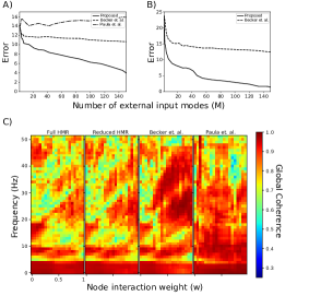
Figure 2: A) Error computed for Hindmarsh-Rose model for $a=1$,$b=3$, $c=1$, $d=5$, $r=0.006$, $s=4$, $x0=-1.6$, $K11=0.5$, $K21=0.5$, $Inhibition-excitationratio(IER)\in(0,2.5)$, $\mu\in(0,2.5)$, $\sigma=0.4$, $w\in(0,1)$, $M\in(1,150)$, $\tau_{1}=0.05ms$, $\tau_{2}=1ms$ and $\tau_{3}=2.5ms$ B) Error computed for VanderPol model for $a=0.1$, $K\in(0,0.5)$, $\mu\in(0,0.5)$, $w\in(0,1)$, $\tau_{1}=\tau_{2}=\tau_{3}=0.05ms$, $\sigma=0.4$ and $M\in(1,150)$ C) Global coherence spectra is plotted for varying node interaction levels in the large-scale network for Hindmarsh-Rose model with $\mu=1.75$ and $IER=2.0$ for full and reduced cases (30 modes).

We simulated a network of three nodes with each functional unit in a node is governed by 1) Van der Pol (VDP) oscillator or 2) HMR neurons. We select the node connection matrix of the given form

$$W=\begin{bmatrix}0&1&1\\ -1&0&1\\ -1&-1&0\end{bmatrix}\times w$$

where $w$ is a scalar in the range $0$ to $1$ representing negligible node interaction to strong node interaction. We also considered different values of $K$ for VDP (and Inhibition-excitation ratio, $IER=\frac{K_{12}}{K_{11}}$ for HMR) and for different values of mean current $\mu$. For validating reduced system with $M$ modes, we compare the Global Coherence (GC) evaluated using the complete system ($C_{p}$) with GC evaluated using the reduced system ($R_{p}$) using the following equation.

$$error(M)=\sqrt{\sum_{p=<f,w,K,\mu>}^{T}\left(\begin{array}[]{c}C_{p}-R_{p}\end{array}\right)^{2}}$$ (92)

where $f$ is frequency and $T$ is total number of pairs $<f,w,K,\mu>$. GC is computed between mean activities of each node. For the reduced system, the mean activity of each node is the mean of individual excitable systems’ activities estimated using (3) without the residual.

As $M$ increases, error in proposed reduction process decreases more rapidly as compared to previous approaches (Figure 2A & B) for both large-scale networks using Van der-Pol and Hindmarsh-Rose models as nodes, thus, validating our reduction approach. For Van der-Pol model, reduction proposed in Sanz-Leon et al. (2015) generated numerical instability during simulation. Global coherence calculated from proposed reduction for an exemplar parameter space matches closely with the original system unlike heuristic approaches (Figure 2C). We further validate our framework by showing the reproduction of time-series of mean-field activity of each HMR and VDP node (Figure 3) for several different parameters spaces.

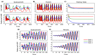
Figure 3: Preservation of mean-field activity of each node in the reduced model with 30 modes for Hindmarsh-Rose model A) $w=0.5$, $\mu=2.5$, $IER=0.8$ and $K11=0.5$ B) $w=0.5$, $\mu=2.5$, $IER=0.8$ and $K11=30$ and C) $w=0.5$, $\mu=2.5$, $IER=2.5$ and $K11=30$ and for Vander-Pol model D) $w=0.5$, $K=0.1$ and $\mu=1$ and E) $w=0.5$, $K=0.1$ and $\mu=0.1$.

In Stefanescu and Jirsa (2008), local-interaction between state-variables was facilitated via the mean field activity of the node which by itself is a small-scale network. In the reduced model this interaction was preserved as the input to state variable of mode $i$ was characterized via mode-specific output of the node ($\sum_{j=1}^{M}A_{ij}\alpha_{j}$) governed by matrix $A$ which is obtained as a part of reduction. However, in the case of the large-scale network of these reduced nodes the input to state-variable of mode $i$ of node $m$ was either the activity of state-variable of mode $i$ from other nodes Becker et al. (2015) or it was the sum of activities of state-variables of all modes from other nodes Sanz-Leon et al. (2015). In this paper, the input to mode $i$ of node $m$ is derived by projecting the long-range interaction term of complete large-scale network to modes of the external input. Thus, our proposed scheme preserves the original long range interaction (Figure 2 and Figure 3).

In summary, we propose a generalized scheme for reduction of the dynamics of a large-scale network into lower dimensional mode description based on properties of the external input. Obviously, any such reduction lowers the computational complexity. However an important point to note is a model’s benefit is not necessarily limited to mimicking the complex dynamics of real-world system. For example, a detailed model of the cortical layer will be highly informative Markram et al. (2015), but not necessarily insightful for explaining the cortical interactions during a specific behavioral task. How do we develop task-specific insights from a high dimensional data with minimal assumptions will be critical question for future studies and how they could profit from our proposed formalism. Our approach is best-placed to application where task inevitably involves reduction from high-dimensional state space to functionally well defined lower dimensional modes. Such problems are also not necessarily exclusively brain specific, but also pertinent for climate dynamics, traffic problems, or anywhere dynamical systems are driven by external time varying and distributed input and the approach presented in this article may be insightful for a wide range of scientific disciplines.

This research was funded by NBRC core and the grants Ramalingaswami fellowship (BT/RLF/Re-entry/31/2011) and Innovative Young Bio-technologist Award (IYBA) (BT/07/IYBA/2013) from the Department of Biotechnology (DBT), Ministry of Science & Technology, Government of India to AB. DR is supported by the Ramalingaswami fellowship (BT/RLF/Re-entry/07/2014) and DST extramural grant (SR/CSRI/21/2016). We also thank Prof. Michael Breakspear for helpful comments and discussions.

Appendix A: Reduction coefficients for Van der Pol oscillator network

$$A_{ij} =\int_{I^{\prime}}g(I^{\prime})v_{j}(I^{\prime})dI^{\prime}\int_{I}v_{i}^{+}dI$$

$$a_{i} =a\int_{I}v_{i}^{3}(I)v_{i}^{+}(I)dI$$

$$II_{i} =\int_{I}Iv_{i}^{+}(I)dI$$

$g(I)$ is the pdf of external input.

Appendix B: Reduction coefficients for Hindmarsh-Rose neuronal network

$$A_{ij} =\int_{I^{\prime}}g1(I^{\prime})v1_{j}(I^{\prime})dI^{\prime}\int_{I}v1_{i}^{+}(I)dI$$

$$B_{ij} =\int_{I^{\prime}}g2(I^{\prime})v2_{j}(I^{\prime})dI^{\prime}\int_{I}v1_{i}^{+}(I)dI$$

$$C_{ij} =\int_{I^{\prime}}g1(I^{\prime})v1_{j}(I^{\prime})dI^{\prime}\int_{I}v2_{i}^{+}(I)dI$$

$$a1_{i} =a\int_{I}v1_{i}^{3}(I)v1_{i}^{+}(I)dI$$

$$a2_{i} =a\int_{I}v2_{i}^{3}(I)v2_{i}^{+}(I)dI$$

$$b1_{i} =b\int_{I}v1_{i}^{2}(I)v1_{i}^{+}(I)dI$$

$$b2_{i} =b\int_{I}v2_{i}^{2}(I)v2_{i}^{+}(I)dI$$

$$c1_{i} =c\int_{I}v1_{i}^{+}(I)dI$$

$$c2_{i} =c\int_{I}v2_{i}^{+}(I)dI$$

$$d1_{i} =d\int_{I}v1_{i}^{2}(I)v1_{i}^{+}(I)dI$$

$$d2_{i} =d\int_{I}v2_{i}^{2}(I)v2_{i}^{+}(I)dI$$

$$p1_{i} =rsx_{0}\int_{I}v1_{i}^{+}(I)dI$$

$$p2_{i} =rsx_{0}\int_{I}v2_{i}^{+}(I)dI$$

$$II1_{i} =\int_{I}Iv1_{i}^{+}(I)dI$$

$$II2_{i} =\int_{I}Iv2_{i}^{+}(I)dI$$

$g1(I)$ and $g2(I)$ are the pdfs of external input to excitatory and inhibitory sub-populations respectively.

References

• (1) D. A. HSIEH, The Journal of Finance 46, 1839.
• Charbonneau et al. (2017) P. Charbonneau, J. Kurchan, G. Parisi, P. Urbani,  and F. Zamponi, Annual Review of Condensed Matter Physics 8, 265 (2017).
• Song et al. (2010) C. Song, Z. Qu, N. Blumm,  and A.-L. Barabási, Science 327, 1018 (2010).
• Antoulas et al. (2010) A. C. Antoulas, C. A. Beattie,  and S. Gugercin, in Efficient Modeling and Control of Large-Scale Systems (Springer, 2010).
• Deco et al. (2008) G. Deco, V. K. Jirsa, P. A. Robinson, M. Breakspear,  and K. Friston, PLoS Comp Biol 4, e1000092 (2008).
• Stefanescu and Jirsa (2008) R. A. Stefanescu and V. K. Jirsa, PLOS Comp Biol 4, 1 (2008).
• Haken (1983) H. Haken, Synergetics: An Introduction, 3rd ed., Springer Series in Synergetics (Springer-Verlag, 1983).
• Becker et al. (2015) R. Becker, S. Knock, P. Ritter,  and V. Jirsa, PLOS Comp Biol 11, 1 (2015).
• Sanz-Leon et al. (2015) P. Sanz-Leon, S. A. Knock, A. Spiegler,  and V. K. Jirsa, NeuroImage 111, 385 (2015).
• van der Pol (1920) B. van der Pol, Radio Rev 1, 701 (1920).
• Hindmarsh and Rose (1984) J. L. Hindmarsh and R. M. Rose, Proc. R. Soc. London B: Biological Sciences 221, 87 (1984).
• Markram et al. (2015) H. Markram, E. Muller, S. Ramaswamy, M. W. Reimann, M. Abdellah, C. A. Sanchez, A. Ailamaki, L. Alonso-Nanclares, N. Antille, S. Arsever, G. A. A. Kahou, T. K. Berger, A. Bilgili, N. Buncic, A. Chalimourda, G. Chindemi, J.-D. Courcol, F. Delalondre, V. Delattre, S. Druckmann, R. Dumusc, J. Dynes, S. Eilemann, E. Gal, M. E. Gevaert, J.-P. Ghobril, A. Gidon, J. W. Graham, A. Gupta, V. Haenel, E. Hay, T. Heinis, J. B. Hernando, M. Hines, L. Kanari, D. Keller, J. Kenyon, G. Khazen, Y. Kim, J. G. King, Z. Kisvarday, P. Kumbhar, S. Lasserre, J.-V. Le Bé, B. R. C. Magalhães, A. Merchán-Pérez, J. Meystre, B. R. Morrice, J. Muller, A. Muñoz-Céspedes, S. Muralidhar, K. Muthurasa, D. Nachbaur, T. H. Newton, M. Nolte, A. Ovcharenko, J. Palacios, L. Pastor, R. Perin, R. Ranjan, I. Riachi, J.-R. Rodríguez, J. L. Riquelme, C. Rössert, K. Sfyrakis, Y. Shi, J. C. Shillcock, G. Silberberg, R. Silva, F. Tauheed, M. Telefont, M. Toledo-Rodriguez, T. Tränkler, W. Van Geit, J. V. Díaz, R. Walker, Y. Wang, S. M. Zaninetta, J. DeFelipe, S. L. Hill, I. Segev,  and F. Schürmann, Cell 163, 456 (2015).