Phase Control of Attosecond Pulses in a Train

Abstract

Ultrafast processes in matter can be captured and even controlled by using sequences of few-cycle optical pulses, which need to be well characterized, both in amplitude and phase. The same degree of control has not yet been achieved for few-cycle extreme ultraviolet pulses generated by high-order harmonic generation in gases, with duration in the attosecond range. Here, we show that by varying the spectral phase and carrier-envelope phase (CEP) of a high-repetition rate laser, using dispersion in glass, we achieve a high degree of control of the relative phase and CEP between consecutive attosecond pulses. The experimental results are supported by a detailed theoretical analysis based upon the semiclassical three-step model for high-order harmonic generation.

Keywords: High-order Harmonic Generation, Attosecond Pulse, Carrier Envelope Phase

1 Introduction

Ultrafast phenomena can be studied and even controlled by using sequences of ultrashort pulses [1]. This requires detailed characterization and control of the pulses, including their relative phase. The frontier in pulse duration has moved to the attosecond range using high-order harmonic generation (HHG) in gases [2, 3]. However, the level of characterization and control of sequences of attosecond pulses with a central frequency in the extreme ultraviolet (XUV) spectrum and a duration reaching down to a few cycles [4, 5] is far from reaching that of optical or infrared few-cycle pulses.

The measurement of the CEP of a single attosecond pulse has been discussed theoretically [6] and recently demonstrated using high-order harmonics generated in the vacuum ultraviolet range from a solid [7]. A direct measurement of the CEP in the time domain for XUV pulses is, however, so far not feasible. In contrast, the spectral phase of single attosecond pulses has been determined using cross-correlation techniques such as streaking [8] with, in particular, the FROG-CRAB (Frequency-Resolved Optical Gating-Complete reconstruction of attosecond burst) analysis [9]. The RABBIT (Reconstruction of Attosecond Beating by Interference of Two-photon Transition) technique allows the determination of the average spectral phase of attosecond pulses in a pulse train [10] and is therefore well suited for multi-cycle driving pulses, such that the phase of attosecond pulses does not vary significantly between consecutive pulses, apart from the $\pi$ change, due to the fundamental symmetry of the interaction. The present work focuses on the relative phase change between consecutive attosecond pulses in a short train, with typically, less than five pulses, generated by a few-cycle pulse.

The influence of the chirp of the fundamental field on the spectral width of the high harmonics has been studied previously [11, 12, 13], with the result that the spectral width of the generated harmonics becomes narrower when the fundamental field is positively chirped, due to compensation of the phase modulation due to the generation process, which leads to a negative chirp [14]. It is also well known that control of the fundamental CEP is important when HHG is driven by few-cycle pulses, since the process is sensitive to the electric field oscillations [15, 16, 17]. Changing the CEP may lead to spectral shifts between odd and even orders, or for very short driving pulses, between a modulated spectrum and a quasi-continuum [16, 18]. The generation of single attosecond pulses in particular requires precise control of the laser CEP. The study of HHG with controlled (and variable) CEP has also led to detailed study of interferences between quantum paths originating from the so-called long trajectory contributions [19]. Recently, interference effects have been observed over a broad spectral range when varying the dispersion of CEP-stable few-cycle laser pulses [20, 21, 22].

In the present work, we study HHG in argon gas as a function of chirp and CEP of a high-repetition rate CEP-stable fundamental laser field, propagating through glass with variable thickness. Our experimental study utilizes a state-of-the-art 200 kHz, CEP-stabilized, 6.5 fs, 850 nm laser system, based upon optical parametric chirped-pulse amplification (OPCPA) [23, 20]. The excellent stability and control regarding intensity, spectral phase and CEP of this system allows us to perform a detailed study of HHG as a function of dispersion. High-order harmonics are generated in a high-pressure gas jet, favoring the contribution of the short trajectory [24]. The harmonic spectra as a function of glass thickness, present complex interference patterns [20, 21] over a large (40 eV) bandwidth. To understand these structures, we develop an analytical multiple pulse interference model, based upon the semi-classical description of HHG [25, 26, 27], which we validate by comparing with calculations based upon the time-dependent Schrödinger equation (TDSE) [28, 29]. Combined with experimental parameters, such as precise measurements of the fundamental phase [30], our model reproduces accurately the complex interference pattern observed in the experiment, which allows us to deduce the characteristics of the underlying attosecond pulse train, including the phase difference between consecutive attosecond pulses. By finely tuning the dispersion of the fundamental field, we demonstrate control of the relative phase and CEP of consecutive pulses in a train.

2 Experimental method and results

2.1 Experimental setup

The laser used in our experiment is a few-cycle, 200 kHz repetition rate, CEP stabilized OPCPA laser system [31]. The system provides 6 $\mathrm{\mu}$J pulses with a duration of $<7$ fs. The CEP error is measured in an $f$–$2f$ interferometer to be 400 mrad (integrated over two pulses), which corresponds to a timing jitter of the carrier of 160 attosecond, i.e. 12% of one half laser cycle. The pulse duration is measured by a dispersion scan characterization method which uses second harmonic generation in a thin crystal [see figure 1 and [32]].

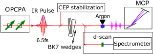
Figure 1: Experimental Setup. The dispersion of a few-cycle IR pulse from a CEP stabilized 200 kHz OPCPA system is controlled with a BK7 glass wedge pair. The IR pulses drive dispersion controlled HHG in argon. With a flip mirror, the pulse can be characterized via a dispersion scan (d-scan) method.

The laser pulses are focussed tightly, using an achromat with a focal length of 5 cm, into a high pressure argon gas jet, where HHG takes place [see figure 1]. The length of the medium is estimated to be slightly larger that 50 $\mu$m and the gas pressure right in front of the nozzle orifice to be approximately 1 bar. The high-pressure gas jet was designed to optimize phase matching of the short trajectory harmonics in these tight focussing geometrical conditions [24]. After passing through a 200 nm thick Al filter in order to block the infrared radiation (IR), the harmonics are detected by a flat-field XUV-spectrometer, consisting of an XUV-grating and a MCP detector. The dispersion, including obviously the CEP, of the few-cycle IR driving pulses is varied using the same motorized BK7-glass wedge pair that is used for the d-scan IR pulse characterization. The induced group delay dispersion (GDD) by transmission trough BK7 is equal to 40 fs²/mm at 850 nm. The laser compressor, consisting of chirped mirrors and a wedge pair, is set up in order to precompensate transmission through air, glass (entrance window, and achromat) such that the shortest pulse in the HHG interaction region is obtained at the position called “zero glass insertion”. In order to obtain good signal-to-noise ratios, each harmonic spectrum is acquired by integrating over about 200 000 shots (1 second).

2.2 Experimental results

Figure 2: Experimental XUV-spectra as a function of dispersion. Two inserts indicate fundamental temporal intensity profiles at i1) 750 $\mu$m, and i2) zero glass insertion. The horizontal fringes are spaced with about $28\,\mathrm{\mu m}$, corresponding to a $\pi$ shift of the fundamental field CEP.

The key result of this work is presented in figure 2 which shows the harmonic spectrum (17th to 41st harmonic) obtained in argon gas as a function of glass insertion from the BK7 wedge pair. The corresponding GDD is indicated on the right axis. The strongest HHG signal and highest cut-off is observed for an almost Fourier-transform limited IR pulse at zero glass insertion. The harmonic signal also decreases significantly for orders above the 29th or photon energy larger than 45 eV, due to the proximity of the Cooper minimum in the photoionization of argon, which affects the recombination step in the single-atom response [33]. The signal decreases for large GDDs (glass insertion of $\pm$ 0.7 mm) due to the decrease in IR-pulse intensity. Harmonic generation can, however, be observed at large glass insertion, an effect that we attribute to the compression of some spectral parts of the complex IR pulse at these large dispersion values, as retrieved from our d-scan measurements. The harmonics, are spectrally broader for negative GDD than for positive GDD, in agreement with previous results [13, 11, 21].

In addition to the large-scale spectral features, two different interference patterns can be observed. The most striking pattern is visible over the whole spectral range and consists of almost horizontal fringes, separated by $\approx$ 28 $\mu$m BK7-glass which corresponds to a $\pi$ shift of the CEP of the driving pulse. The slope of these fringes varies from slightly positive at negative GDD to negative at insertion values larger than 0.3 mm. As shown in more detail below, the change of slope and asymmetry with respect to dispersion, as well as the effect on the harmonic spectral width mentioned above, is due to the interplay between the chirp inherited from the fundamental spectral properties, and that induced by the generation process. At a GDD corresponding to $\approx$ 300 $\mu$m of glass insertion, both effects cancel each other, leading to spectrally narrow harmonics and horizontal CEP-fringes. At larger insertions, around $\pm$750 $\mu$m, vertical interference fringes can be observed. We attribute this effect to attosecond pulse interferences induced by the double pulse structure of the chirped fundamental pulse in these conditions, as shown in the calculations presented below.

3 Theoretical method and results

3.1 TDSE calculations

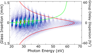
Figure 3: Calculated XUV-spectra as a function of dispersion for Gaussian pulses by solving TDSE. The red lines represent the position of the classical cut-off; the green curves are the calculated position where the harmonics are spectrally narrowed, by solving $s(\Omega)=0$ according to (16).

To understand our results, we first solve the TDSE in the single-active-electron approximation [28] with an argon model atom [34]. We assume a fundamental Gaussian pulse with 6.2 fs pulse duration (FWHM of the temporal intensity profile) at zero glass insertion. The fundamental wavelength is 850 nm, which corresponds to the center of mass of the experimental spectrum, and the peak intensity at Fourier-transform limited pulse duration is 2.3$\times 10^{14}$ W/cm². HHG spectra are obtained by Fourier transforming the time-dependent acceleration of the dipole moment. We do not include propagation in the nonlinear medium. A soft mask, which absorbs the electronic wavefunction, is placed about 1.7 nm (32 a.u.) away from the nucleus. This distance is chosen using classical electron trajectory calculations so that for the shortest pulse duration, i.e. the highest intensity, the long electron trajectories, which travel farther that the short trajectories, are absorbed, thus not contributing to the emission of radiation. However, for lower intensity (when the glass insertion is not zero), the mask is too far away and only leads to partial absorption of the long trajectories, which therefore influence the HHG spectra.

Figure 3 presents theoretical results obtained with the TDSE method. Many of the features observed in the experiment are qualitatively reproduced. CEP fringes are observed throughout the spectra, with a dispersion-dependent slope. The Cooper minimum of argon is found at about 50 eV (31st harmonic). When the dispersion becomes positive, the harmonic peaks get narrower. The spectra in figure 2 and figure 3 are, however, different at large positive or negative dispersion. The close-to-vertical fringes observed in the TDSE result cannot be explained by the distortion of the fundamental pulse [see insert in figure 2(i1)], as suggested for the experimental result. We believe that they might be due to the influence of the long trajectory, as discussed further below.

3.2 Multiple interference model

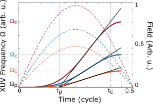
Figure 4: Fundamental electric field (dashed) and calculated emitted XUV frequency (solid) due to the short trajectory as a function of time for three intensities $I$ (red line), $I/2$ (blue line), $I/4$ (orange line). $\Omega(t)$ is obtained by solving the classical equation of motion for the electron in the field. Only one half-cycle of the fundamental is represented. $\Omega_{\mathrm{p}}$ is the frequency corresponding to the ionization energy $I_{\mathrm{p}}$, while $\Omega_{\mathrm{c}}$ refers to the intensity-dependent classical cut-off. $t_{\mathrm{p}}=0.18$ cycle and $t_{\mathrm{c}}=0.40$ cycle are the intersections of the tangent to the XUV frequency curve with $\Omega=\Omega_{\mathrm{p}}$ and $\Omega_{\mathrm{c}}$ respectively.

We now describe our model, which is based upon interferences between attosecond pulses [20, 35]. The attosecond light emission is described at the single atom level using the semi-classical three-step model [25, 36]. In this model, an electron tunnels through the potential barrier at a time $t_{\mathrm{i}}$, oscillates in the laser field, returns to the core at time $t_{\mathrm{r}}$ where it may recombine back to the ground state. The time of return $t_{\mathrm{r}}$ is related to $t_{\mathrm{i}}$ through the following equation:

$$\sin(\omega t_{\mathrm{r}})-\sin(\omega t_{\mathrm{i}})-\omega(t_{\mathrm{r}}-t_{\mathrm{i}})\cos(\omega t_{\mathrm{i}})=0,$$ (1)

where $\omega$ is the laser frequency. The kinetic energy acquired by the electron in the field is

$$E_{\mathrm{kin}}=2U_{\mathrm{p}}\left[\cos(\omega t_{\mathrm{r}})-\cos(\omega t_{\mathrm{i}})\right]^{2},$$ (2)

where $U_{\mathrm{p}}$ is the ponderomotive energy, equal to $e^{2}E_{0}^{2}/4m\omega^{2}$, where $e$, $m$ are the electron charge and mass and $E_{0}$ is the amplitude of the electromagnetic field. The kinetic energy reaches a maximum (a cutoff) equal to $3.2U_{\mathrm{p}}$. All energies (except the cutoff) can be reached by two trajectories, the short and the long respectively. In this article, we only consider the short trajectory. Figure 4 shows the generated XUV frequency [$\Omega=(E_{\mathrm{kin}}+I_{\mathrm{p}})/\hbar$] as a function of return time for a half-cycle of the laser field for three different laser intensities. $\Omega_{\mathrm{p}}$ is the first frequency above threshold, equal to $I_{\mathrm{p}}/\hbar$ and $\Omega_{\mathrm{c}}$ is the cut-off frequency. The generated XUV frequency $\Omega$ varies approximately linearly with time of return in the HHG plateau region, as shown by comparing the exact solutions to their tangents taken at $(\Omega_{\mathrm{c}}+\Omega_{\mathrm{p}})/2$ (black lines). Remarkably, the tangent curves all cross the threshold and (intensity-dependent) cutoff frequency at the same time, $t_{\mathrm{p}}$ and $t_{\mathrm{c}}$ respectively. $t_{\mathrm{p}}$ and $t_{\mathrm{c}}$ are calculated numerically and found to be equal to 0.18 and 0.40 cycles of the IR laser field. The physical reason for this interesting geometrical property is that the return time is independent of intensity (1), while the kinetic energy is proportional to it (2). This leads us to approximate the time of return $t(\Omega)=t_{\mathrm{r}}$ as,

$$t(\Omega)\approx t_{\mathrm{p}}+\frac{t_{\mathrm{c}}-t_{\mathrm{p}}}{\Omega_{\mathrm{c}}-\Omega_{\mathrm{p}}}(\Omega-\Omega_{\mathrm{p}}),$$ (3)

The spectral phase $\Phi(\Omega)$ of the attosecond emission is the integral of $t(\Omega)$ so that

$$\Phi(\Omega)=t_{\mathrm{p}}(\Omega-\Omega_{\mathrm{p}})+\frac{t_{\mathrm{c}}-t_{\mathrm{p}}}{\Omega_{\mathrm{c}}-\Omega_{\mathrm{p}}}\frac{(\Omega-\Omega_{\mathrm{p}})^{2}}{2},$$ (4)

where we have dropped a constant phase term. Since $\hbar(\Omega_{\mathrm{c}}-\Omega_{\mathrm{p}})=3.2U_{\mathrm{p}}$, which is proportional to the intensity $I$ within the half-cycle,

$$\Phi(\Omega)=t_{\mathrm{p}}(\Omega-\Omega_{\mathrm{p}})+\frac{\gamma}{I}(\Omega-\Omega_{\mathrm{p}})^{2},$$ (5)

where

$$\gamma=\frac{\hbar(t_{\mathrm{c}}-t_{\mathrm{p}})I}{6.4U_{\mathrm{p}}}=\frac{(t_{\mathrm{c}}-t_{\mathrm{p}})\hbar\varepsilon_{0}cm\omega^{2}}{3.2e^{2}}.$$ (6)

where $\varepsilon_{0}$ and $c$ are the vacuum permittivity and speed of light in vacuum respectively. From figure 4, using an experimental laser cycle of 2.8 fs, we determine $t_{\mathrm{p}}=0.45\,\mathrm{fs}$ and $\gamma=1.0\times 10^{12}\,\mathrm{fs^{2}\mathrm{W/cm}^{2}}$.

Equation (5) contradicts the approximation $\Phi(\Omega)=\alpha I$, often used in the literature [37, 38]. Taking the derivative of $\Phi(\Omega)$ with respect to $I$, we obtain

$$\alpha=\frac{\partial\Phi}{\partial I}=-\frac{\gamma}{I^{2}}(\Omega-\Omega_{\mathrm{p}})^{2}.$$ (7)

For a given frequency $\Omega$, $\alpha$ depends on the laser intensity. However, $\alpha$ becomes intensity-independent, if $(\Omega-\Omega_{\mathrm{p}})\propto I$, i.e. if the return time is kept constant when the intensity changes. For example, for the middle point of the plateau region, $\Omega=(\Omega_{\mathrm{c}}+\Omega_{\mathrm{p}})/2$, $\alpha$ does not depend on the laser intensity since $\Omega-\Omega_{\mathrm{p}}=(\Omega_{\mathrm{c}}-\Omega_{\mathrm{p}})/2\propto I$.

Our model calculates the XUV field by summing the contributions from all of the half cycles

$$\tilde{A}(\Omega)=\sum_{m}|A_{m}(\Omega)|e^{i[\Omega t_{m}+m\pi+\Phi_{m}(\Omega)]},$$ (8)

where $m$ is the index of the half cycle of the fundamental field, with $m=0$ denoting that with the maximum amplitude, $t_{m}$ is the time of the zero-crossing of the electric field for the $m$-th half cycle, which corresponds to the emission time of the lowest plateau harmonic (corresponding to 0 in figure 4). $|A_{m}|$ is the modulus of the spectral amplitude of the attosecond pulse emitted due to the $m$-th half cycle and $\Phi_{m}(\Omega)$ is the spectral phase, describing the intensity-dependent chirp of the attosecond emission [see (5)]. The sign flip between consecutive attosecond pulses is described by the $m\pi$ term in the argument of the exponential. Both CEP and dispersion of the fundamental pulse are transferred to the attosecond pulses via the variation of the timing $t_{m}$. The XUV spectrum $A_{m}(\Omega)$ is assumed to have a super-Gaussian shape for every attosecond pulse $m$ spanning from the threshold $\Omega_{\mathrm{p}}$ to the cutoff frequency $\Omega_{\mathrm{c}}$, which depends on the intensity of the fundamental field at $t_{m}$ [$I_{m}=I(t_{m})$]. The integrated power spectrum $\int_{0}^{\infty}|A_{m}(\Omega)|^{2}d\Omega$ of the attosecond pulses is assumed to vary with the laser intensity as the ionization rate, which can be determined from the Ammosov–Delone–Kraĭnov approximation [39]. The spectral intensity $|A_{m}(\Omega)|^{2}$ is weighted by the probability for recombination, extracted from [40]. The spectral phase is obtained as explained in (5) for each half cycle.

To determine the time $t_{m}$ and the corresponding intensity $I_{m}$, we calculate the field of the driving IR-pulse. We perform two calculations, using experimental and Gaussian pulses. For the experimental pulses, the spectral phase and amplitude are determined using the d-scan measurements [figure 2], from which the electric field for a given glass insertion $\ell$ is obtained by Fourier transform. The absolute fundamental CEP is not known. However, the variation of the CEP with glass insertion is included by propagating the field through glass.

For Gaussian pulses, we use an analytical formulation. We express the fundamental field as

$$E(t)=E_{\mathrm{max}}\exp\left(-\frac{t^{2}}{2\tau^{2}}\right)\sin\left(\omega t+\varphi+\frac{b}{2}t^{2}\right),$$ (9)

where $E_{\mathrm{max}}$ is the maximum amplitude, $\tau$ the pulse duration at $1/e$, $b$ the chirp coefficient and $\varphi$ a global phase, assumed to be between $-\pi/2$ and $\pi/2$. The CEP is usually defined for a cosine wave. Since we here use a sine wave, $\varphi$ is not the CEP but half $\pi/2$ shifted from it. The times at which the electric field goes to zero, $t_{m}$, are such that

$$t_{m}=-\frac{\omega}{b}\pm\sqrt{\frac{\omega^{2}}{b^{2}}-\frac{2\varphi}{b}+\frac{2m\pi}{b}}.$$ (10)

Only the times with the plus sign are physically acceptable. The intensity for the half-cycle $m$ is given by

$$I_{m}=I_{\mathrm{max}}\exp(-t_{m}^{2}/\tau^{2}),$$ (11)

where $I_{\mathrm{max}}$ is laser intensity at the peak of the envelope. Finally, we relate the chirp rate $b$, the laser intensity at the peak of the envelope $I_{\mathrm{max}}$ and the pulse duration $\tau$ to the glass insertion $\ell$ through the formulas:

$$b=\frac{2k^{\prime\prime}\ell}{a^{2}\tau_{\mathrm{FL}}^{4}};I_{\mathrm{max}}=\frac{I_{\mathrm{FL}}}{a};\tau=\tau_{\mathrm{FL}}a$$ (12)

with

$$a=\sqrt{1+\frac{4k^{\prime\prime 2}\ell^{2}}{\tau_{\mathrm{FL}}^{4}}}.$$ (13)

Here $\tau_{\mathrm{FL}}$ is the pulse duration at $1/e$ for a Fourier transform limited pulse; $k^{\prime\prime}$ is the dispersion in glass at the fundamental frequency (40.09 fs²/mm); $I_{\mathrm{FL}}$ is the maximum laser intensity for the shortest pulse duration. The fundamental global phase $\varphi$ is related to the difference between phase and group velocity and is taken to be $k\ell-k^{\prime}\ell\omega$, with the restriction that it should be included between $-\pi/2$ and $\pi/2$.

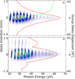
Figure 5: Calculated XUV-spectra as a function of dispersion: (a) Analytical calculation using the interference model for Gaussian pulses and (b) Numerical simulation {from the multiple pulse interference model} with the pulse measured from the experiment. The red lines represent the position of the classical cut-off; the green curves are the calculated position where the harmonics are spectrally narrowed, by solving $s(\Omega)=0$ according to (16).

The results of the model are shown in figure 5 for Gaussian (a) and experimental pulses (b). Comparing figure 3 and figure 5(a), we find that most TDSE features are very well reproduced by our interference model, except for the interference fringes observed at large dispersion in the TDSE result. Since only the short trajectory contribution is included in our model, we believe that the reason for the (close-to-vertical) interference pattern in the TDSE spectra is the contribution of the long trajectories. Figure 5(a) reproduces well the main features of the experimental spectra [figure 2]. In this case, the vertical fringes are due to the double pulse structure of the experimental pulse [see insert in figure 2(i1)].

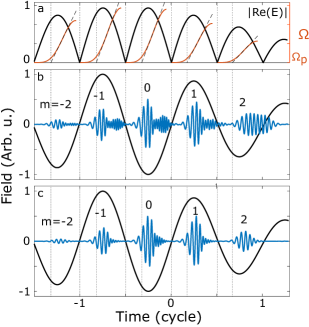
Figure 6: (a)Fundamental electric field (black) and emitted XUV frequency (red) due to the short trajectory as a function of time. All of the relevant half-cycles are indicated. Generated XUV field (blue) (b) calculated using the TDSE and (c) obtained with our interference model.

Our model, validated by comparison with the TDSE and the experimental results, can now be used to deduce the attosecond pulse train in the time domain. Figure 6(a) shows the generated XUV frequencies at each laser half-cycle during the laser pulse, while figure 6(b,c) presents the attosecond pulse trains obtained at zero fundamental dispersion using TDSE and our model for a Gaussian pulse respectively. Five attosecond pulses with different chirp and timing can be identified. Their duration varies from 220 as at the center of the fundamental pulse to 780 as at the edges according to the TDSE simulation. The three central XUV bursts in figure 6(b) exhibit a minimum in the middle. The minimum results from the Cooper minimum at 50 eV in the photoionization cross-section. This spectral minimum (and the spectral phase variation associated with it, see [41]) is transferred to the temporal profile of the XUV bursts through the time–energy link inherently present in the HHG process. For the model [figure 6(c)], the Cooper minimum is not as obvious as the result from TDSE, which can be attributed to a higher yield of high energy harmonics in the latter calculation. For the short trajectory contribution, early time corresponds to low energy [41], resulting in positive chirp of the attosecond pulses [10]. The XUV bursts emitted before and after the three central ones, do not exhibit this minimum since the instantaneous intensity is too low to generate harmonics with high orders.

3.3 Analytical derivation of the phase of the attosecond pulses

The excellent agreement between the TDSE calculations [figure 3] and our multiple interference model using a Gaussian pulse [figure 5(a)], as well as between experiment [figure 2] and the model using experimental pulses [figure 5(b)] motivated us to extract an approximate analytical expression for the phase of the attosecond pulses in order to understand the structure of the fringe pattern. For small dispersion, i.e. when $|(\varphi-m\pi)b|/\omega^{2}\ll 1$, $t_{m}$ can be approximated by

$$t_{m}\approx-\frac{\varphi-m\pi}{\omega}-\frac{b(\varphi-m\pi)^{2}}{2\omega^{3}}.$$ (14)

The phase $\Phi_{m}$ can be approximated by

$$\Phi_{m}(\Omega)\approx t_{\mathrm{p}}(\Omega-\Omega_{\mathrm{p}})+\frac{\gamma}{I_{\mathrm{max}}}\left[1+\left(\frac{\varphi-m\pi}{\omega\tau}\right)^{2}\right](\Omega-\Omega_{\mathrm{p}})^{2}$$ (15)

where we have used $I_{m}\approx I_{\mathrm{max}}(1-t_{m}^{2}/\tau^{2})$, keeping only the first term in (14). Both $t_{\mathrm{p}}$ and $\gamma$ do not depend on $m$. Separating the contributions which are $m$-independent, dependent on $m$ and $m^{2}$, (8) becomes

$$\tilde{A}(\Omega)=e^{iz(\Omega)}\sum_{m}|A_{m}(\Omega)|e^{imf(\Omega)+im^{2}s(\Omega)},$$ (16)

where the functions $z$, $f$ and $s$ are given by

$$z(\Omega)= -\frac{\Omega\varphi}{\omega}\left(1+\frac{b\varphi}{2\omega^{2}}\right)+t_{\mathrm{p}}(\Omega-\Omega_{\mathrm{p}})+\frac{\gamma}{I_{\mathrm{max}}}(\Omega-\Omega_{\mathrm{p}})^{2}$$ (17a)

$$f(\Omega)= \pi+\frac{\pi\Omega}{\omega}+\varphi\kappa(\Omega)$$ (17b)

$$s(\Omega)= -\frac{\pi\kappa(\Omega)}{2}.$$ (17c)

with

$$\kappa(\Omega)=\frac{b\pi\Omega}{\omega^{3}}-\frac{2\pi\gamma}{\omega^{2}\tau^{2}I_{\mathrm{max}}}(\Omega-\Omega_{\mathrm{p}})^{2}.$$ (17r)

The function $z(\Omega)$ represents the phase of the “central” attosecond pulse in the train. The first two terms are unimportant since a linear variation in frequency leads to a shift in the temporal domain. The last term gives rise to group delay dispersion (GDD) which leads to temporal broadening, and which is inversely proportional to the intensity [10, 42]. Furthermore, $z(\Omega)$ does not influence the spectrum $|\tilde{A}(\Omega)|^{2}$ and cannot be measured in our experiment. Nonlinear correlation schemes such as streaking [43], RABITT [2] or autocorrelation [44] are required for characterizing attosecond pulses.

The function $f(\Omega)$ describes how the CEP affects the interference between attosecond pulses, and consequently the emission at harmonic frequencies. Setting $\varphi=0$, we obtain constructive interferences when $f(\Omega)=2q\pi$, i.e. $\Omega=(2q+1)\omega$. The position of the constructive interferences is found to vary with the CEP through the chirp of the fundamental pulse and the dipole phase. The term $b\varphi/\omega^{2}$ leads to a small change in periodicity ($\delta t=\pi/\omega=T/2$ is changed into $T/2+b\varphi T/2\omega^{2}$) and therefore of the frequency difference between consecutive harmonics. The dipole phase leads to a small increase of the periodicity (and therefore decrease in harmonic spacing) at high frequency.

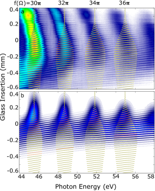
Figure 7: A magnified area of (a) figure 2 and (b) figure 5(a), showing harmonics 31 to 37. The thin lines are the solutions to $f(\Omega)=30\pi$, $32\pi$, $34\pi$ and $36\pi$ as a function of glass insertion $\ell$.

Finally, the function $s(\Omega)$ partly spoils the interference structure, leading to “sub-harmonic” features [35]. The zeros of $s(\Omega)$ give the position where harmonics are sharpest. It is indicated by the green lines in figure 3 and figure 5(a) in perfect agreement with the numerical calculations. The harmonics are narrowest for positive chirp, since it compensates for the effect of the dipole phase ($\gamma>0$ for the short trajectory). Negative fundamental chirp on the other hand leads to spectral broadening of the harmonics, which eventually overlap and interfere [21]. The function $s(\Omega)$ affects the timing between consecutive attosecond pulses, due to glass dispersion and induced by the generation process. Assuming $\varphi=0$ and neglecting the dipole phase, for example, the difference of time between consecutive attosecond pulses is equal to $\delta t_{m}=T/2-(2m-1)\pi^{2}b/2\omega^{3}$, which increases or decreases, depending on the sign of $b$, during the laser pulse. Similarly, when $b=0$, the dipole phase will lead to a varying time difference between two consecutive attosecond pulses, equal to $T/2+2\pi(2m-1)\gamma(\Omega-\Omega_{\mathrm{p}})/\omega^{2}\tau^{2}I_{\mathrm{max}}$. We can make a “perfect” train, i.e. equidistant attosecond pulses, over a certain spectral range where $s(\Omega)\approx 0$, by canceling the dipole phase variation with a small positive fundamental chirp [12].

Both $f(\Omega)$ and $s(\Omega)$ [through $\kappa(\Omega)$] depend on fundamental laser parameters such as chirp ($b$), pulse duration ($\tau$) and intensity ($I_{\mathrm{max}}$). In the limit of long pulses and no fundamental chirp, $\kappa(\Omega)\approx 0$, the pulse train becomes regular and the phase difference between consecutive attosecond pulses is equal to $\pi$ (The harmonic spectrum then consists of odd-order harmonics).

4 Discussion

4.1 Analysis of the interference fringes

In figure 7(a,b), representing magnified areas in figure 2 and figure 5(a) respectively, we plot the position of $f(\Omega)=2n\pi$ as a function of glass insertion $\ell$. Here, we simulated HHG with a slightly blue-shifted fundamental wavelength in order to mimic the experimental conditions. In the region $\ell=-0.6$ to +0.1 mm, the results fit well both the position of the interference fringes and their tilt with frequency as well as the dispersion-dependent width of the harmonics, which validates our model. For the trivial case of two interfering pulses, the interference pattern is governed by the function $f(\Omega)+s(\Omega)=2n\pi$. As soon as the APT includes more than two pulses, the interference pattern is essentially imposed by the condition $f(\Omega)=2n\pi$, as exemplified in figure 7. Note that $f(\Omega)$ is dominated by the term $\pi\Omega/\omega$, so that $s(\Omega)$ varies with frequency much more slowly than $f(\Omega)$. For dispersion larger than $0.1$ mm, however, we believe that the interference pattern cannot only be described by the simple condition $f(\Omega)=2n\pi$ [see (16)].

This analysis provides a “recipee” for retrieving the phase difference between consecutive pulses in the train, which is imprinted in the interference fringes (figure 2). This technique should work well for a few attosecond pulses (two or three) but becomes more complex as the number of pulses increases. An alternative method is the FROG-CRAB technique [9], which, in principle, allows for the retrieval of the pulse train.

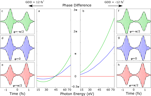
Figure 8: Phase difference $\Delta\phi(\Omega)$ between the 0th and 1st attosecond pulse in the pulse train for (a) positive and (b) negative glass insertion (dispersion equal to $\pm 12\,\mathrm{fs^{2}}$, equivalent to $\pm 300\,\mathrm{\mu m}$ of glass insertion); Simulated 0th and 1st attosecond pulses, after spectrally filtering through a 100-nm thick chromium foil, for positive (c–e) and negative (f–h) glass insertion. The red, blue and green lines have obtained for $\varphi=\pi/2,0$ and $-\pi/2$ respectively. An additional absolute phase is applied to the pulses to maintain the CEP of the first attosecond pulse ($m=0$) the same, for visualizing the phase variation of the second pulse ($m=1$).

4.2 Phase control of attosecond pulses in a train

An important result of our derivation is that we can simply determine how the spectral phase of attosecond pulses varies from the zeroth to the first pulse (apart from the $\pi$ phase jump and the half-cycle time delay). We have

$$\Delta\phi(\Omega)=\left(\varphi-\frac{\pi}{2}\right)\kappa(\Omega).$$ (17s)

We show in figure 8(a,b) this phase difference as a function of XUV photon energy for different fundamental global phase ($\varphi$) and two different glass insertions. For positive $b$, the phase difference goes through a stationary point where the effects of fundamental dispersion and dipole phase variation compensate each other [$\kappa(\Omega)=0$, green line in figure 5(a)]. At the stationary point, the influence of $\varphi$ on $\Delta\phi$ is very small, which means that $\Delta\phi$ is very robust against any CEP fluctuations. Even when for $\varphi\neq\pi/2$, the variation of $\Delta\phi$ with $\varphi$ for any frequency remains less than $\pi$. In addition, for any fundamental CEP, the variation of $\Delta\phi$ across the spectrum is small (at most $\approx\pi$), so that, as discussed previously, the harmonics are spectrally narrow, thus leading to regular attosecond pulse trains. In contrast, negative fundamental dispersion leads to a larger variation with CEP and across the spectrum [figure 8(b)]. Here, $\Delta\phi$ can vary from 0 to almost $3\pi$ at the cutoff by changing the fundamental CEP. In this case, the harmonics are spectrally broad, and strongly CEP-dependent. The corresponding pulse trains are irregular.

The spectral phase control demonstrated above allows us to control the relative CEP of attosecond pulses in a train. These two quantities are not independent, since the electric field is related to the complex spectral amplitude by Fourier transform. More specifically, the relative CEP of the attosecond pulse can be controlled by changing the relative spectral phase. To demonstrate this, we present calculated consecutive pairs of attosecond pulses with different CEPs equal to $-\pi/2$, 0 and $\pi/2$ in figure 8(c–e) and (f–h). This calculation uses the multiple pulse interference model for our experimental conditions, with the addition that a 100 nm thick chromium filter [45] is numerically introduced to select a narrow spectral range from 30 eV to 50 eV. A global absolute phase is also added to make the first pulse like a “cosine” wave (CEP equal 0), so that the phase variation of the second pulse is clearly visualized. For positive dispersion (c-d), the pulses do not change much with fundamental CEP, and the CEP difference between the two pulses is close to $\pi$. For negative dispersion (f-h), the CEP of the second pulse is equal to $\pi$ for $\varphi=\pi/2$; $\pi/2$ for $\varphi=0$ and 0 for $\varphi=-\pi/2$. Changing the fundamental CEP in this case gives us control of the relative CEP between consecutive attosecond pulses. The CEP control achieved by this method depends on many parameters, such as intensity, dispersion and selected spectrum.

5 Conclusion

In summary, we have studied high-order harmonic generation in argon driven by a few-cycle 200 kHz optical parametric chirped pulse amplifier system, as a function of fundamental CEP and dispersion. The spectra exhibit a complex pattern of interference fringes when the dispersion is changed. These structures are well reproduced by simulations based on the solution of the time-dependent Schrödinger equation as well as by a multiple-pulse interference model, based upon the semi-classical approximation. Using an analytical expression for the phase of attosecond pulses in a train, we show that the relative spectral phase and CEP of consecutive pulses in an attosecond-pulse train generated from a few cycle CEP-stable fundamental field can be controlled by the dispersion and CEP of the driving IR pulse. Positive dispersion leads to pulse trains which are robust against fundamental CEP variation, with reproducible attosecond waveforms from one pulse to the next. In contrast, negative dispersion leads to pulse trains with variable and controllable relative atto CEP. The fundamental dispersion and CEP provide an important control knob for the attosecond pulse trains. In some applications, e.g. interferometry [46], robust and stable attosecond pulse trains, which can be obtained using positive dispersion, are needed.

In other type of applications, e.g. pump/probe or coherent control [1], it is important to control the relative phase between two pulses. In this case, negative dispersion and variable fundamental CEP should be used. The level of control achieved in the present work extends the applicability of many coherent spectroscopy techniques, previously limited to the optical range, to shorter time scale and higher photon energy.

References

References

- [1] Tannor D J, Kosloff R and Rice S A 1986 J. Chem. Phys. 85 5805
- [2] Paul P, Toma E, Breger P, Mullot G, Augé F, Balcou P, Muller H and Agostini P 2001 Science 292 1689
- [3] Hentschel M, Kienberger R, Spielmann C, Reider G A, Milosevic N, Brabec T, Corkum P, Heinzmann U, Drescher M and Krausz F 2001 Nature 414 509
- [4] López-Martens R, Varjú K, Johnsson P, Mauritsson J, Mairesse Y, Salières P, Gaarde M B, Schafer K J, Persson A, Svanberg S, Wahlström C G and L’Huillier A 2005 Phys. Rev. Lett. 94 033001
- [5] Sansone G, Benedetti E, Calegari F, Vozzi C, Avaldi L, Flammini R, Poletto L, Villoresi P, Altucci C, Velotta R, Stagira S, Silvestri S D and Nisoli M 2006 Science 314 443
- [6] He P L, Ruiz C and He F 2016 Phys. Rev. Lett. 116 203601
- [7] Garg M, Zhan M, Luu T T, Lakhotia H, Klostermann T, Guggenmos A and Goulielmakis E 2016 Nature 538 359
- [8] Kienberger R, Hentschel M, Uiberacker M, Spielmann C, Kitzler M, Scrinzi A, Wieland M, Westerwalbesloh T, Kleineberg U, Heinzmann U, Drescher M and Krausz F 2002 Science 297 1144
- [9] Quéré F, Itatani J, Yudin G L and Corkum P B 2003 Phys. Rev. Lett. 90 073902
- [10] Mairesse Y, de Bohan A, Frasinski L J, Merdji H, Dinu L C, Monchicourt P, Breger P, Kovaev M, Taïeb R, Carré B, Muller H G, Agostini P and Salières P 2003 Science 302 1540
- [11] Chang Z, Rundquist A, Wang H, Christov I, Kapteyn H and Murnane M 1998 Phys. Rev. A 58 R30
- [12] Mauritsson J, Johnsson P, López-Martens R, Varjú K, Kornelis W, Biegert J, Keller U, Gaarde M B, Schafer K J and L’Huillier A 2004 Phys. Rev. A 70 R021801
- [13] Kim H T, Kim I J, Hong K H, Lee D G, Kim J H and Nam C H 2004 J. Phys. B: At., Mol. Opt. Phys. 37 1141
- [14] Varjú K, Mairesse Y, Carré B, Gaarde M, Johnsson P, Kazamias S, López-Martens R, Mauritsson J, Schafer K, Balcou P et al. 2005 J. Mod. Opt. 52 379
- [15] Nisoli M, Sansone G, Stagira S, De Silvestri S, Vozzi C, Pascolini M, Poletto L, Villoresi P and Tondello G 2003 Phys. Rev. Lett. 91 213905
- [16] Sola I, Mével E, Elouga L, Constant E, Strelkov V, Poletto L, Villoresi P, Benedetti E, Caumes J P, Stagira S, Vozzi C, Sansone G and Nisoli M 2006 Nat. Phys. 2 319
- [17] Haworth C A, Chipperfield L E, Robinson J S, Knight P L, Marangos J P and Tisch J W 2007 Nat. Phys. 3 52
- [18] Baltuska A, Uiberacker M, Goulielmakis E, Kienberger R, Yakovlev V S, Udem T, Hansch T W and Krausz F 2003 IEEE J. Sel. Topics Quantum Electron. 9 972
- [19] Sansone G, Benedetti E, Caumes J P, Stagira S, Vozzi C, Pascolini M, Poletto L, Villoresi P, Silvestri S D and Nisoli1 M 2005 Phys. Rev. Lett. 94 193903
- [20] Rudawski P, Harth A, Guo C, Lorek E, Miranda M, Heyl C, Larsen E, Ahrens J, Prochnow O, Binhammer T, Morgner U, Mauritsson J, L’Huillier A and Arnold C L 2015 Eur. Phys. J. D 69 70
- [21] Holgado W, Hernández-García C, Alonso B, Miranda M, Silva F, Plaja L, Crespo H and Sola I 2016 Phys. Rev. A 93 013816
- [22] Holgado W, Hernández-García C, Alonso B, Miranda M, Silva F, Varela O, Hernández-Toro J, Plaja L, Crespo H and Sola I J 2017 Phys. Rev. A 95 063823
- [23] Krebs M, Hädrich S, Demmler S, Rothhardt J, Za�r A, Chipperfield L, Limpert J and Tünnermann A 2013 Nat. Photonics 7 555
- [24] Heyl C, Coudert-Alteirac H, Miranda M, Louisy M, Kovacs K, Tosa V, Balogh E, Varjú K, L’Huillier A, Couairon A et al. 2016 Optica 3 75
- [25] Corkum P 1993 Phys. Rev. Lett. 71 1994
- [26] Kulander K C, Schafer K J and Krause J L 1992 Time-Dependent Studies of Multiphoton Processes Atoms in Intense Laser Fields (San Diego: Academic Press)
- [27] Lewenstein M, Balcou P, Ivanov M, L’Huillier A and Corkum P 1994 Phys. Rev. A 49 2117
- [28] Schafer K J 2009 Numerical Methods in Strong Field Physics vol Strong Field Laser Physics (Springer) p 111 ISBN 978-0-387-40077-8
- [29] Carlström S 2017 Sub-cycle control of strong-field processes on the attosecond timescale (Lund : Division of Atomic Physics, Department of Physics, Lund University, 2017) ISBN 978-9-177-53117-3
- [30] Miranda M, Arnold C L, Fordell T, Silva F, Alonso B, Weigand R, L’Huillier A and Crespo H 2012 Opt. Express 20 18732
- [31] Harth A, Guo C, Cheng Y C, Losquin A, Miranda M, Mikaelsson S, Heyl C M, Prochnow O, Ahrens J, Morgner U, L’Huillier A and Arnold C L Manuscript under preparation
- [32] Miranda M, Fordell T, Arnold C, L’Huillier A and Crespo H 2012 Opt. Express 20 688
- [33] Higuet J, Ruf H, Thiré N, Cireasa R, Constant E, Cormier E, Descamps D, Mével E, Petit S, Pons B, Mairesse Y and Fabre B 2011 Phys. Rev. A 83 053401
- [34] Kulander K and Rescigno T 1991 Comput. Phys. Commun. 63 523
- [35] Mansten E, Dahlström J M, Mauritsson J, Ruchon T, L’Huillier A, Tate J, Gaarde M B, Eckle P, Guandalini A, Holler M, Schapper F, Gallmann L and Keller U 2009 Phys. Rev. Lett. 102 083002
- [36] Schafer K J, Yang B, DiMauro L F and Kulander K C 1993 Phys. Rev. Lett. 70 1599
- [37] Lewenstein M, Kulander K C, Schafer K J and Bucksbaum P H 1995 Phys. Rev. A 51 1495
- [38] Balcou P, Dederichs A S, Gaarde M B and L’Huillier A 1999 J. Phys. B 32 2973
- [39] Ammosov M, Delone N and Krainov V 1986 Sov. Phys. JETP 64 1191
- [40] Samson J and Stolte W 2002 J. Electron Spectrosc. Relat. Phenom. 265
- [41] Schoun S, Chirla R, Wheeler J, Roedig C, Agostini P, DiMauro L, Schafer K and Gaarde M 2014 Phys. Rev. Lett. 112 153001
- [42] Varjú K, Mairesse Y, Agostini P, Breger P, Carré B, Frasinski L J, Gustafsson E, Johnsson P, Mauritsson J, Merdji H, Monchicourt P, L’Huillier A and Salières P 2005 Phys. Rev. Lett. 95 243901
- [43] Kienberger R, Goulielmakis E, Uiberacker M, Baltuka A, Yakovlev V, Bammer F, Scrinzi A, Westerwalbesloh T, Kleineberg U, Heinzmann U, Drescher M and Krausz F 2004 Nature 427 817
- [44] Tzallas P, Skantzakis E, Nikolopoulos L, Tsakiris G and Charalambidis D 2011 Nat. Phys. 7 781
- [45] Henke B, Gullikson E and Davis J 1993 At. Data Nucl. Data Tables 54 181
- [46] Isinger M, Squibb R, Busto D, Zhong S, Harth A, Kroon D, Nandi S, Arnold C L, Miranda M, Dahlström J, Lindroth E, Feifel R, Gisselbrecht M and L’Huillier A 2017 Science (arXiv:1709.01780 [physics.atom–ph])