How order melts after quantum quenches

Abstract

Injecting a sufficiently large energy density into an isolated many-particle system prepared in a state with long-range order will lead to the melting of the order over time. Detailed information about this process can be derived from the quantum mechanical probability distribution of the order parameter. We study this process for the paradigmatic case of the spin-1/2 Heisenberg XXZ chain. We determine the full quantum mechanical distribution function of the staggered subsystem magnetization as a function of time after a quantum quench from the classical Néel state. This provides a detailed picture of how the Néel order melts and reveals the existence of an interesting regime at intermediate times that is characterized by a very broad probability distribution.

Introduction. —

A fundamental objective of quantum theory is to determine probability distribution functions of observables in given quantum states. In few-particle systems the time evolution of such probability distributions provides a lot of useful information beyond what is contained in the corresponding expectation values. Recent advances in cold-atom experiments have made possible not only the study of non-equilibrium time evolution of (almost) isolated many-particle systems Langen2015 ; Altman2015 ; kww-06 ; GM:col_rev02 ; hacker10 ; tetal-11 ; shr-12 ; cetal-12 ; langen13 ; MM:Ising13 ; ronzheimer13 ; zoran1 ; lev2017 , but given access to the full quantum mechanical probability distributions of certain observables HLSI08 ; KPIS10 ; KISD11 ; GKLK12 ; Greiner . This provides an opportunity to gain new insights about the coherent dynamics of many-particle quantum systems. One intriguing question one may ask is how order melts, or forms, when an isolated many-particle system is driven across a phase transition. Related questions have been studied in solids, but there one essentially deals with open quantum systems and has access to very different observables, see e.g. Hill ; Cavalieri . The basic setup we have in mind is as follows. Let us consider a system of quantum spins with Hamiltonian $H$ that is initially prepared in a state with density matrix $\rho(0)$. In this state there is long-range order characterized by a local order parameter ${\cal O}=\sum_{j=1}^{L}{\cal O}_{j}$, where $j$ runs over the sites of the lattice and ${\cal O}_{j}$ is a local operator. We are interested in the probability distribution $P_{A}$ of the order parameter ${\cal O}_{A}$ in a contiguous subsystem of linear size $|A|$

$$P_{A}(m,t)={\rm Tr}\big{[}\rho(t)\delta({\cal O}_{A}-m)\big{]}.$$ (1)

Here $\rho(t)$ is the density matrix of the system at time $t$ and $P_{A}(m,t)$ is the probability that the subsystem order parameter ${\cal O}_{A}$ takes the value $m$ in the state $\rho(t)$. We are interested in cases where the system is initially well ordered at all length scales and $P_{A}(m,t)$ is therefore narrowly peaked around the average ${\cal O}_{A}$. Under time evolution the order melts and at late times and large subsystem sizes $P_{A}(m,t)$ is believed to approach a Gaussian distribution centred around zero Deutsch1991 ; Srednicki1994 ; Rigol2008 ; Rigol2007 ; Cassidy2011 ; Caux2013 ; Ilievski2015 . The question of interest is how $P_{A}(m,t)$ evolves as a function of time and subsystem size $|A|$. Varying the latter provides information about how well the system is ordered at length scale $|A|$.

We find that when the initially ordered system is quenched well into the unbroken symmetry phase of the Hamiltonian, the (local) order quickly disappears and the PDF acquires a simple Gaussian shape. In contrast, when the quantum quench is to an energy density where Hamiltonian eigenstates retain short-range order, the PDF exhibits a complex structure both at finite times and in the steationay state. In the following we focus on the example of the spin-$1/2$ Heisenberg XXZ chain, but note that the picture we put forward is general and has a wide range of applicability.

Model and Setup. —

We investigate the time evolution of antiferromagnetic (short-ranged) order after a quantum quench in the spin-$1/2$ XXZ chain

$$H_{\Delta}=\sum_{j}S^{x}_{j}S^{x}_{j+1}+S^{y}_{j}S^{y}_{j+1}+\Delta\,S^{z}_{j}S^{z}_{j+1}.$$ (2)

Here $S^{\alpha}_{j}$ are spin-$1/2$ operators acting on the site $j$ and we restrict our analysis to the range $\Delta>0$. The phase diagram of (2) is well established: at $T=0$ there is a BKT phase transition at $\Delta=1$ that separates a quantum critical phase at $\Delta<1$ and an antiferromagnetically ordered phase at $\Delta>1$. At any finite temperature the antiferromagnetic order melts. The Hamiltonian (2) is invariant under rotations by an arbitrary angle around the z-axis, translations by one site, and rotations around the x-axis by 180 degrees. In the thermodynamic limit at $\Delta>1$ and zero temperature the last symmetry gets broken spontaneously and one of the two degenerate ground states $|{\rm GS}^{\pm}_{\Delta}\rangle$, characterized by equal but opposite expectation values of the staggered magnetization per site, gets selected. In the Ising limit $\Delta\to\infty$ the ground states become the classical Néel states, i.e. $|{\rm GS}^{+}_{\infty}\rangle=|\cdots\uparrow\downarrow\uparrow\downarrow\cdots\rangle$ and $|{\rm GS}^{-}_{\infty}\rangle=|\cdots\downarrow\uparrow\downarrow\uparrow\cdots\rangle$. In order to investigate the melting of antiferromagnetic order we consider the following quantum quench protocol: (i) we prepare the system in the classical Néel state $|\Phi_{0}\rangle=|{\rm GS}^{+}_{\infty}\rangle$, which exhibits saturated antiferromagnetic long-ranged order; (ii) We consider unitary time evolution with Hamiltonian $H_{\Delta}$. The state of the system at time $t$ is thus $|\Phi_{t}\rangle=\exp(-iH_{\Delta}t)|\Phi_{0}\rangle$. This quench is integrable Pozsgay:13a ; FE_13b ; FCEC_14 and exact results on the stationary state are available neel_overlap ; QANeel ; XXZung ; XXZunglong ; Ilievski2015 ; IQNB . We employ the infinite Time-Evolving Block-Decimation (iTEBD) algorithm iTEBD1 ; iTEBD2 to obtain a very accurate description of $|\Phi_{t}\rangle$ in the thermodynamic limit. However, the growth of the bipartite entanglement entropy limits the time window accessible by this method. Retaining up to $\chi_{max}=1024$ auxiliary states, we are able to reach a time $t_{max}\simeq 12$ without significant error ($\lesssim 10^{-3}$).

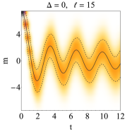
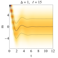
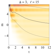
Figure 1: Density plot of $\widetilde{P}_{\ell}(m,t)$ with $m\in[-\ell/2,\ell/2]$ and $t\in[0,12]$ for a subsystem size $\ell=15$, after a quench from the Néel state $|{\rm GS}^{+}_{\infty}\rangle$ to $\Delta=0,\,1,\,2,\,3$. The full line represents the expectation value $\bar{m}(t)$, the dashed lines are the standard deviation from the average, namely $\bar{m}(t)\pm\sigma(t)$.

PDF dynamics. —

Detailed information on how the antiferromagnetic order melts as the system evolves in time is provided by the probability distribution of the staggered subsystem magnetisation $M_{\ell}\equiv\sum_{j=1}^{\ell}(-1)^{j}S^{z}_{j}$

$$P_{\ell}(m,t) \equiv \langle\Phi_{t}|\delta(M_{\ell}-m)|\Phi(t)\rangle\ ,$$ (3)

$$= \sum_{r\in\mathbb{Z}}\widetilde{P}_{\ell}(m,t)\delta\big{(}m-r-(1-(-1)^{\ell})/4\big{)}\ ,$$

where second line follows from the fact that the eigenvalues of $M_{\ell}$ are half-integer numbers. We note that the probabilities satisfy the normalisation condition $\sum_{m=-\ell/2}^{\ell/2}\widetilde{P}_{\ell}(m,t)=1$. The initial Néel state is an eigenstate of the staggered subsystem magnetization $M_{\ell}$ and concomitantly the probability distribution is a delta function $P_{\ell}(m,0)=\delta(m-\ell/2)$. This reflects the long-range magnetic order in the initial state. In Fig. 1 we show the evolution of $P_{\ell}(m,t)$ in time obtained by iTEBD for subsystem size $\ell=15$ and several values of the interaction strength $\Delta$ in the “post-quench” Hamiltonian (2).

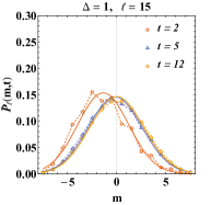
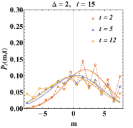
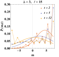
Figure 2: Snapshots of the rescaled PDF in Fig. 1 at fixed times $t=5,\,10,\,15$. The numerical data (symbols/dashed lines) are compared to the Gaussian approximation (4) (full lines).

We observe that the probability distribution depends strongly on $\Delta$: for small values of $\Delta$ the antiferromagnetic short-ranged order melts quickly and $P_{\ell}(m,t)$ is narrowly peaked around its average, which exhibits a damped oscillatory behaviour around zero BPGDA09 . The behaviour for $\Delta\gtrsim 2$ is very different: short-ranged order persists for some time while the probability distribution broadens and becomes more symmetric in $m$. This nicely chimes with the expectation (see below) that in the stationary state reached at late times the probability distribution to become symmetric in $m$. In Fig. 2 we plot the weights of $P_{\ell}(m,t)$ at several times and compare them to a Gaussian approximation based on the first two moments $\bar{m}(t)=\langle\Phi_{t}|M_{\ell}|\Psi_{t}\rangle$, $\sigma^{2}(t)=\langle\Phi_{t}|M_{\ell}^{2}|\Psi_{t}\rangle-\bar{m}^{2}(t)$

$$P_{\ell}(\mu,t)=\frac{1}{\sqrt{2\pi\sigma(t)}}\exp\left\{-\frac{[\mu-\bar{m}(t)]^{2}}{2\sigma(t)}\right\}.$$ (4)

We see that at $\Delta=0$ the probability distribution is approximately Gaussian at all times, while for $\Delta=2,3$ it exhibits a pronounced even/odd structure at short times and even at the latest times shown is strongly non-Gaussian.

“Small”- $\Delta$ regime. —

At small values of $\Delta$ and short and intermediate times we can use a time-dependent self-consistent mean-field approximation to determine the evolution of $P_{\ell}(m,t)$. We first map the Hamiltonian (2) to a model of spinless fermions by means of a Jordan-Wigner transformation, where we use the positive (negative) z-direction in spin space as quantization axis for even (odd) sites (see Supplementary material). This results in a spinless fermion Hamiltonian

$$H_{\Delta}=\sum_{j}\frac{1}{2}\left[c^{\dagger}_{j}c^{\dagger}_{j+1}+{\rm h.c.}\right]+\Delta\,n_{j}(1-n_{j+1}),$$ (5)

where $n_{j}=c^{\dagger}_{j}c_{j}$ and $\{c_{j},c^{\dagger}_{k}\}=\delta_{j,k}$. The staggered subsystem magnetization maps to $M_{\ell}=\sum_{j=1}^{\ell}(1/2-n_{j})$, while the initial Néel state maps to the fermion vacuum $|\Psi_{0}\rangle=|0\rangle$. Our self-consistent approximation corresponds to the replacement

$$n_{j}n_{j+1} \rightarrow \left[\langle c^{\dagger}_{j}c^{\dagger}_{j+1}\rangle_{t}c_{j+1}c_{j}-\langle c^{\dagger}_{j+1}c_{j}\rangle_{t}c^{\dagger}_{j}c_{j+1}+{\rm h.c.}\right]$$ (6)

$$+ \langle n_{j}\rangle_{t}n_{j+1}+\langle n_{j+1}\rangle_{t}n_{j},$$

which leads to an explicitly time-dependent Hamiltonian $H_{\rm MF}(t)$, cf. Ref. SotiriadisCardy, . The expectation values in (6) are calculated self-consistently $\langle.\rangle_{t}=\langle\Psi_{t}|.|\Psi_{t}\rangle$, where

$$|\Psi_{t}\rangle=T\exp\left[-i\int_{0}^{t}dt^{\prime}H_{\rm MF}(t^{\prime})\right]|0\rangle.$$ (7)

Following Ref. Groha, we can express the characteristic function of $P_{\ell}(m,t)$ as a determinant of a $2\ell\times 2\ell$ matrix (see Supplementary material), which is easily evaluated numerically. This provides us with exact results at $\Delta=0$ for all times, cf. Fig. 3, and a highly accurate short-time approximation even for $\Delta=3$ as is shown in Fig. 4.

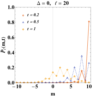
Figure 3: $\widetilde{P}_{\ell}(m,t)$ for $\ell=20$ at times $t=0,0.5,1$ after a quantum quench from a classical Néel state to a Heisenberg chain with $\Delta=0$. Lines are exact results (see main text) and symbols are obtained by iTEBD.

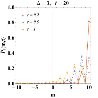
Figure 4: $\widetilde{P}_{\ell}(m,t)$ for $\ell=20$ at times $t=0$, $0.5$, $1$ after a quench from the classical Néel state to a Heisenberg chain with $\Delta=4$. Lines are obtained by the self-consistent fermionic mean-field approximation and the symbols are iTEBD results.

Late times and large $\Delta$. —

We now turn to the behaviour at late times after the quench. The stationary state is characterized by a finite correlation length $\xi(\Delta)$. On length scales $\ell\lesssim\xi(\Delta)$ we expect short-ranged antiferromagnetic order to remain, while it will have melted at scales $\ell>\xi(\Delta)$. We also expect the spin-rotational symmetry by 180 degrees around the x-axis to be restored in the stationary state as we are dealing with a one dimensional system with short-range interactions. The situation is completely analogous to that at finite temperatures – in fact adding a very small integrability-breaking term to the Hamiltonian would result in a steady state that is very close to the thermal state of the XXZ chain QANeel . In contrast to the steady state after our quench, the probability distribution of the staggered subsystem magentization at finite temperature $P_{\ell}(m,\beta)$ can be computed by matrix product state methods and for the aforementioned reasons it is instructive to consider it. Results for two values of $\Delta$ are shown in Fig. 5. We see that the probability distributions are symmetric in $m$, reflecting the unbroken symmetry of rotations around the x-axis by 180 degrees. At $\Delta=4$ we further observe that when the subsystem size exceeds the thermal correlation length $\xi_{\Delta}(\beta)$ antiferromagnetic short-ranged order melts and we obtain a Gaussian probability distribution centred around $m=0$. On the other hand, for $\ell\lesssim\xi_{\Delta}(\beta)$ the probability distribution is very broad and peaked at the maximal values $\pm\ell/2$, signalling the presence of both kinds of antiferromagnetic short-ranged order. For $\Delta=1$ the thermal correlation length is smaller than one lattice site in the temperature regime shown, which is why no traces of short-range order are visible and the probability distribution is a Gaussian centred around $m=0$.

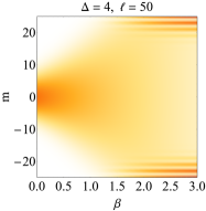
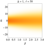
Figure 5: Density plot of the PDF for the XXZ chain at finite temperature $1/\beta$ for subsystem size $\ell=50$ and $\Delta=4$ (left panel); $\Delta=1$ (right panel).

The large-$\Delta$ regime is characterized by a low density of excitations and it is therefore possible to understand the behaviour observed above by combining a $1/\Delta$-expansion with a linked-cluster expansion along the lines of Refs EK:finiteT, ; JEK, ; GKE, ; PT10, ; ST12, ; CEF1, ; CEF2, ; SE:Ising, ; sine-Gordon, . As the physics we wish to describe is not tied to integrability, and the non-integrable case is easier to discuss, we focus on the latter. We consider the regime $\Delta\gg 1$ and break integrability by adding a small perturbation to the Heisenberg Hamiltonian, e.g. consider time evolution under $H=H_{\Delta}+\Delta^{-n}V$, where $n$ is a positive integer and $V$ some perturbation involving short-ranged spin-spin interactions that has the same symmetries as $H_{\Delta}$. We define linked clusters following the general formalism of Ref. EK:finiteT, and then implement a $1/\Delta$-expansion through a unitary transformation $\widetilde{H}=e^{iS}He^{-iS}$ SchriefferWolf , see the Supplementary Material for details. The result is an expansion of the stationary state density matrix of the form

$$\rho_{\rm SS}=\sum_{j\geq 0}\rho_{\rm SS}^{(j)}\ ,\ \rho_{\rm SS}^{(j)}={\cal O}\big{(}e^{-\beta_{\rm eff}j\Delta/2}\big{)}\ ,$$ (8)

where $\rho_{\rm SS}^{(j)}$ are given as power series in $1/\Delta$. The leading term in the expansion is $\rho_{\rm SS}^{(0)}=\frac{1}{2}\sum_{\sigma=\pm}|{\rm GS}_{\Delta}^{\sigma}\rangle\langle{\rm GS}_{\Delta}^{\sigma}|$, where $|{\rm GS}_{\Delta}^{\sigma}\rangle$ are the two ground states of the model at anisotropy $\Delta$. The small parameter $e^{-\beta_{\rm eff}\Delta/2}$ is proportional to the density of domain-wall excitations over the ground states at large $\Delta$. The expansion (8) of the steady-state density matrix leads to a corresponding expansion of the probability distribution of the staggered subsystem magnetization $P_{\ell}(m,\infty)=\sum_{j}P^{(j)}_{\ell}(m)$ (see Supplemental Material)

$$P^{(0)}_{2\ell}(m) = \delta(\ell-|m|)\left[\frac{1}{2}-\frac{2\ell+1}{8\Delta^{2}}\right]+\delta(\ell-1-|m|)\frac{1}{4\Delta^{2}}$$ (9)

$$+ \delta(\ell-2-|m|)\frac{2\ell-1}{8\Delta^{2}}+o(\Delta^{-2}),$$

$$P^{(1)}_{2\ell}(m) = e^{-\frac{\beta_{\rm eff}\Delta}{2}}I_{0}(\beta_{\rm eff})\bigg{[}\frac{1-\ell}{2}\delta(\ell-|m|)$$ (10)

$$+ \sum_{j=1}^{\ell}\delta(\ell-j-|m|)\bigg{]}+\dots,$$

where the dots denote subleading terms in $1/\Delta$. The expansions (10) hold as long as the subsystem size $2\ell$ is small compared to the correlation length in $\rho_{\rm SS}$ and establish that for large anisotropies $\Delta$ the probability distribution in the steady state is symmetric in $m$ and close to the average over the two ground states. In addition there is an exponentially suppressed ”background” contribution arising from a dilute gas of domain walls.

“Symmetrization” of the PDF in time. —

A characteristic feature of the time-evolution of $P_{\ell}(m,t)$ is that it becomes increasingly symmetric in $m$. In order to ascertain the associated time scale in the most interesting large-$\Delta$ regime it is useful to compare the probabilities for $M_{\ell}$ to be maximal ($\ell/2$) or minimal ($-\ell/2$) respectively. Results for $\Delta=6$ are shown in Fig. 6.

Figure 6: Weights $\tilde{P}_{\ell}(m,t)$ for $\ell=10$ and a quench from the classical Néel state to a Heisenberg chain with $\Delta=6$. We observe a linear growth (decrease) in time of the weights for $m=-\ell/2$ ($m=\ell/2$), indicating that the symmetrization of the PDF is driven by ballistic propagation of quasi-particles.

We see that $P_{\ell}(-\ell/2,t)$ grows linearly in time, while $P_{\ell}(\ell/2,t)$ shows a corresponding linear decrease. For the integrable XXZ chain the associated velocity is expected to be the maximal group velocity of elementary excitations over the stationary state BEL . In presence of weak integrability-breaking interactions in the large-$\Delta$ regime we expect qualitatively similar prethermal behaviour prethermal .

Conclusions. —

We have considered the full quantum mechanical probability distribution of the staggered subsystem magnetization $P_{\ell}(m,t)$ after a quantum quench from a classical Néel state to the spin-1/2 Heisenberg XXZ chain. We have shown that $P_{\ell}(m,t)$ provides detailed information how short-range antiferromagnetic order melts and have shown how to understand our numerical findings by analytical approaches valid in certain limits. Our setup should be realizable in cold-atom experiments like the ones by the Harvard group Greiner .

Acknowledgments. —

We are grateful to P. Calabrese, A. De Luca and M. Fagotti for stimulating discussions and to the Erwin Schrödinger International Institute for Mathematics and Physics for hospitality and support during the programme on Quantum Paths. M.C. thanks the Galileo Galilei Institute in Florence for hospitality during the workshop “Entanglement in quantum systems”. This work was supported by the the European Union’s Horizon 2020 under the Marie Sklodowska-Curie grant agreement No. 701221 NET4IQ (M.C and F.H.L.E.), the EPSRC under grant EP/N01930X (F.H.L.E.), the National Science Foundation under Grant No. NSF PHY-1748958 (F.H.L.E.) and by the BMBF and EU-Quantera via QTFLAG (M.C.).

*

Appendix A SUPPLEMENTARY MATERIAL

A.1 Self-consistent time dependent mean-field approximation

In the small-$\Delta$ regime the quench dynamics of the Heisenberg XXZ chain can be analyzed by means of a self-consistent time-dependent mean-field theory SotiriadisCardy as we will now demonstrate. For convenience we rotate the spin-quantization axis on all odd sites, which maps the classical Néel state on the saturated ferromagnetic state with all spins up. This transformation is induced by $P=\prod_{j\;{\rm odd}}\sigma^{x}_{j}$ and we have

$$|\Psi_{0}\rangle \equiv P|\Phi_{0}\rangle=|\uparrow\uparrow\dots\uparrow\rangle,$$

$$S_{\ell} \equiv PM_{\ell}P=\sum_{j=1}^{\ell}S^{z}_{j},$$ (1)

while the Hamiltonian maps onto

$$H^{\prime}_{\Delta} \equiv PH_{\Delta}P$$ (2)

$$= \sum_{j}S^{x}_{j}S^{x}_{j+1}-S^{y}_{j}S^{y}_{j+1}-\Delta S^{z}_{j}S^{z}_{j+1}\ .$$

The probability distribution of the staggered subsystem magnetization in the XXZ chain is then expressed as

$$P_{\ell}(m,t)=\langle\Psi_{t}|\delta(S_{\ell}-m)|\Psi_{t}\rangle\ ,\quad|\Psi_{t}\rangle=e^{-iH^{\prime}_{\Delta}t}|\Psi_{0}\rangle\ .$$ (3)

Performing the Jordan-Wigner transformation to spinless fermions $\{c_{i},c^{{\dagger}}_{j}\}=\delta_{ij}$

$$S^{+}_{j}=\prod_{i}^{j-1}(1-2n_{i})c_{i},\quad S^{z}_{j}=\frac{1}{2}-n_{j},$$ (4)

the Hamiltonian becomes (up an unimportant constant)

$$H^{\prime}_{\Delta}=\sum_{j}\frac{1}{2}\left[c^{{\dagger}}_{j}c^{{\dagger}}_{j+1}-c_{j}c_{j+1}\right]+\Delta\,n_{j}\left[1-n_{j+1}\right],$$ (5)

where $n_{i}=c^{{\dagger}}_{i}c_{i}$. The initial state maps onto the fermion vacuum, i.e.

$$|\Psi_{0}\rangle=|0\rangle.$$ (6)

We now decouple the four-fermion interaction in a self-consistent fashion

$$c^{{\dagger}}_{j}c^{{\dagger}}_{j+1}c_{j+1}c_{j} \approx \langle n_{j}\rangle_{t}\,n_{j+1}+\langle n_{j+1}\rangle_{t}\,n_{j}$$

$$- \langle c^{{\dagger}}_{j}c_{j+1}\rangle_{t}\,c^{{\dagger}}_{j+1}c_{j}-\langle c^{{\dagger}}_{j+1}c_{j}\rangle_{t}\,c^{{\dagger}}_{j}c_{j+1}$$

$$+ \langle c^{{\dagger}}_{j}c^{{\dagger}}_{j+1}\rangle_{t}\,c_{j+1}c_{j}+\langle c_{j+1}c_{j}\rangle_{t}\,c^{{\dagger}}_{j}c^{{\dagger}}_{j+1},$$

which leads to a time-dependent mean-field Hamiltonian

$$H_{\rm MF}(t) = \sum_{j}[A_{j}(t)c_{j+1}c_{j}+B_{j}(t)c^{\dagger}_{j+1}c_{j}+{\rm h.c.}]$$ (8)

$$+ \sum_{j}h_{j}(t)n_{j}\ .$$

Here we have defined

$$A_{j}(t) = \frac{1}{2}-\Delta\langle c^{\dagger}_{j}c^{\dagger}_{j+1}\rangle_{t}\ ,$$

$$B_{j}(t) = \Delta\langle c^{\dagger}_{j}c_{j+1}\rangle_{t}\ ,$$

$$h_{j}(t) = \Delta\left[1-\langle n_{j-1}\rangle_{t}-\langle n_{j+1}\rangle_{t}\right].$$ (9)

The expectation values at time $t$ in (LABEL:SCMF) and (9) are calculated self-consistently

$$\langle{\cal O}\rangle_{t} = \langle 0|U^{\dagger}(t){\cal O}U(t)|0\rangle\ ,$$

$$U(t) = T\exp\left[-i\int_{0}^{t}dt^{\prime}H_{\rm MF}(t^{\prime})\right].$$ (10)

The self-consistent mean-field approximation obtained in this way is expected to work well for small values of $\Delta$ and sufficiently short times. As we will see it works quite well even for intermediate values of $\Delta$.

The Heisenberg equations of motion in our self-consistent mean-field approximation are

$$-i\frac{d}{dt}c_{j}(t) = U^{\dagger}(t)[H^{\prime}_{\Delta},c_{j}]U(t)$$ (11)

$$= A_{j-1}^{*}(t)c^{{\dagger}}_{j-1}(t)-A_{j}^{*}(t)c^{{\dagger}}_{j+1}(t)$$

$$- B_{j-1}(t)c_{j-1}(t)-B_{j}^{*}(t)c_{j+1}(t)$$

$$- h_{j}(t)c_{j}(t).$$

It is convenient to cast them in matrix form

$$\frac{d}{dt}{\bf d}(t)=i\,\mathbb{T}_{\Delta}[\mathbb{C}(t)]\cdot{\bf d}(t),$$ (12)

where ${\bf d}^{{\dagger}}\equiv(c^{{\dagger}}_{1},\dots,c^{{\dagger}}_{L},c_{1},\dots,c_{L})$ and we have defined a $2L\times 2L$ correlation matrix $\mathbb{C}(t)$ by

$$\left[\mathbb{C}(t)\right]_{nm}=\langle 0|d_{n}(t)d^{{\dagger}}_{m}(t)|0\rangle.$$ (13)

The time evolution of the correlation matrix is governed by a first-order differential equation

$$\frac{d\mathbb{C}(t)}{dt}=i\mathbb{T}_{\Delta}[\mathbb{C}(t)]\cdot\mathbb{C}(t)-i\mathbb{C}(t)\cdot\mathbb{T}^{{\dagger}}_{\Delta}[\mathbb{C}(t)].$$ (14)

Using that our initial state is the fermion vacuum we have

$$\left[\mathbb{C}(0)\right]_{nm}=\begin{cases}\delta_{n,m}&\text{if }n>L\\ 0&\text{else}.\end{cases}$$ (15)

The correlation matrix at time $t$ can now be straightforwardly obtained by numerically integrating (14). By comparing the results to iTEBD computations we observe very good agreement for small values of $\Delta$. For large values $\Delta>1$ the approximation still gives a fair description of the dynamics at short times $t\lesssim 1$.

A.1.1 Full counting statistics

A nice feature of the self-consistent mean-field approximation described above is that it allows us to determine the probability distribution $P_{\ell}(m,t)$. To that end we define the associated characteristic function by

$$P_{\ell}(m,t) = \int_{-\infty}^{\infty}\frac{d\theta}{2\pi}e^{-im\theta}\ F_{\ell}(\theta,t)\ ,$$

$$F_{\ell}(\theta,t) = \langle 0|U^{\dagger}(t)e^{i\theta S_{\ell}}U(t)|0\rangle\ .$$ (16)

Following Ref. Groha, we can derive a determinant representation for $F_{\ell}(\theta,t)$ that can be efficiently evaluated. We start by introducing Majorana fermion operators by

$$a^{x}_{j}\equiv c^{{\dagger}}_{j}+c_{j},\quad a^{y}_{j}\equiv i(c^{{\dagger}}_{j}-c_{j}).$$ (17)

These have anticommutation relations $\{a^{\alpha}_{i},a^{\beta}_{j}\}=2\delta_{\alpha\beta}\delta_{ij}$ and the observable of interest is bilinear in them

$$S_{\ell}=\sum_{j=1}^{\ell}\frac{i}{2}\,a^{y}_{j}a^{x}_{j}.$$ (18)

Next we introduce an auxiliary reduced density matrix acting on sites $1$,…,$\ell$ by

$$\rho^{\rm aux}_{\ell}=\frac{1}{Z}e^{i\theta S_{\ell}}=\frac{1}{Z}\exp\left[\frac{\theta}{4}{\bf a}^{{\dagger}}\mathbb{W}{\bf a}\right],$$ (19)

where ${\bf a}^{{\dagger}}=(a^{x}_{1},\dots,a^{x}_{\ell},a^{y}_{1},\dots,a^{y}_{\ell})$, $\mathbb{W}=i\sigma^{y}\otimes\mathbb{1}_{\ell}$ and

$$Z={\rm Tr}\left[{\rm e}^{i\theta\sum_{j=1}^{\ell}S^{z}_{j}}\right]=[2\cos(\theta/2)]^{\ell}.$$ (20)

The characteristic function can then be expressed as

$$F_{\ell}(\theta,t)=Z\;{\rm Tr}\big{[}\rho_{\ell}^{\rm aux}\rho_{\ell}(t)\big{]},$$ (21)

where $\rho_{\ell}(t)$ is the reduced density matrix of the subsystem $[1,\ell]$ at time $t$

$$\rho_{\ell}(t)={\rm Tr}_{[\ell+1,L]}\left[U(t)|0\rangle\langle 0|U^{\dagger}(t)\right].$$ (22)

Finally we use an identity for the trace of the product of two Gaussian density matrices proved in Ref. Fagotti,

$${\rm Tr}\left[\rho_{1}\rho_{2}\right]=\sqrt{{\rm det}\left(\frac{1+\Gamma_{1}\Gamma_{2}}{2}\right)}\ ,$$ (23)

where $\Gamma_{j}$ are correlation matrices defined by

$$\left(\Gamma_{j}\right)_{nm}={\rm Tr}\left[\rho_{j}\ a_{m}a_{n}\right]-\delta_{n,m}.$$ (24)

In our case the two correlation matrices are

$$\Gamma^{\rm aux}_{\ell} = \tanh\left(\frac{\theta\mathbb{W}}{2}\right)=\tan\left(\frac{\theta}{2}\right)\mathbb{W}\ ,$$

$$\Gamma_{\ell}(t) = \langle 0|{\bf a}(t){\bf a}^{\dagger}(t)|0\rangle-\mathbb{1}_{2\ell}$$ (25)

$$= \mathbb{M}\mathbb{C}(t)\mathbb{M}^{\dagger}-\mathbb{1}_{2\ell}\ ,$$

where $\mathbb{C}(t)$ is the correlation matrix obtained from (14) and

$$\quad\mathbb{M}=\begin{pmatrix}\mathbb{1}_{\ell}&\mathbb{1}_{\ell}\\ -i\mathbb{1}_{\ell}&i\mathbb{1}_{\ell}\end{pmatrix}.$$ (26)

Our final result for the characteristic function of the probability distribution $P_{\ell}(m,t)$ is thus

$$F_{\ell}(\theta,t)=\big{[}2\cos(\theta/2)\big{]}^{\ell}\sqrt{{\rm det}\left(\frac{1+\Gamma^{\rm aux}_{\ell}\Gamma_{\ell}(t)}{2}\right)}\ .$$ (27)

Combining (27) and (14) we can obtain numerically exact results in the framework of our time-dependent self-consistent mean-field approximation for $F_{\ell}(\theta,t)$ in the thermodynamic limit and large subsystem sizes.

Appendix B Combined linked-cluster and $1/\Delta$ expansions

In the large-$\Delta$ regime we can gain insights about the late time behaviour after the quench by means of combined linked-cluster and $1/\Delta$ expansions. We again carry out a rotation of the spin-quantization axis, which leads us to a Hamiltonian of the form

$$H^{\prime}_{\Delta}=-J\Delta\sum_{j}\tau^{z}_{j}\tau^{z}_{j+1}+2J\sum_{j}\tau^{+}_{j}\tau^{+}_{j+1}+\tau^{-}_{j}\tau^{-}_{j+1}\ .$$ (28)

Here $\tau^{\alpha}_{j}$ are Pauli matrices and we have introduced an energy scale $J$, which should be set to $1/4$ in order to arrive at the conventions used in the main text. In the rotated basis the staggered subsystem magnetization maps onto

$$S^{z}_{\ell}=\frac{1}{2}\sum_{j=1}^{\ell}\tau^{z}_{j}\ ,$$ (29)

and our goal is to calculate

$$P_{\ell}(m,\infty)=\lim_{t\to\infty}\int_{-\infty}^{\infty}\frac{d\theta}{2\pi}\ e^{-im\theta}\langle\uparrow|e^{i\theta S^{z}_{\ell}(t)}|\uparrow\rangle,$$ (30)

where $|\uparrow\rangle$ is the saturated ferromagnetic state. As the physics we are interested in does not rely on the integrability of the spin-1/2 XXZ chain and the non-integrable case is easier to analyze, we proceed by adding a short-ranged integrability-breaking interaction $V$ that does not break any of the discrete symmetries of $H^{\prime}(\Delta)$ and consider

$$H=H^{\prime}_{\Delta}+\Delta^{-n}V\ ,$$ (31)

where $n$ is a positive integer. In the regime $\Delta\gg 1$ we may carry out a $1/\Delta$-expansion following Ref. SchriefferWolf, . We consider a basis transformation of the form

$$\widetilde{H}=e^{iS}He^{-iS}\ ,\quad S=\sum_{j\geq 1}S^{(j)}\Delta^{-j}\ ,$$ (32)

where $S^{(j)}$ are to be chosen in such a way that order by order in the expansion $\widetilde{H}$ commutes with the domain-wall number operator

$$N_{\rm DW}=\frac{1}{2}\sum_{j=1}^{L}1-\tau^{z}_{j}\tau^{z}_{j+1}\ .$$ (33)

The first order term in (32) is

$$S^{(1)}=\sum_{k}\frac{1+i\tau^{z}_{k-1}}{2}\left[\tau^{+}_{k}\tau^{+}_{k+1}-\tau^{-}_{k}\tau^{-}_{k+1}\right]\frac{1+i\tau^{z}_{k+2}}{2}\ .$$ (34)

In the transformed basis the Hamiltonian has the following expansion

$$\widetilde{H} = -J\Delta\sum_{j}\tau^{z}_{j}\tau^{z}_{j+1}+J\sum_{j}\tau^{+}_{j}\tau^{+}_{j+1}+\tau^{-}_{j}\tau^{-}_{j+1}$$

$$- J\sum_{j}\tau^{z}_{j-1}\left[\tau^{+}_{j}\tau^{+}_{j+1}+\tau^{-}_{j}\tau^{-}_{j+1}\right]\tau^{z}_{j+2}+{\cal O}(\Delta^{-1}),$$

and domain wall number is a good quantum number. The ground states of $\widetilde{H}$ are the saturated ferromagnetic states $|\uparrow\rangle=|\uparrow\uparrow\dots\rangle$ and $|\downarrow\rangle=|\downarrow\downarrow\dots\rangle$ with energy $E_{0}=-J\Delta L$ (in the original spin basis these correspond to the two Néel states). Low-lying excited states involve ferromagnetic domain walls. In order to analyze properties at finite but low energy densities by means of the method first introduced in Ref. EK:finiteT, we need to impose open boundary conditions on (LABEL:Htilde) so that excited states with an odd number of domain walls are allowed. To deal with this complication we need to shift the subsystem for which we determine the probability distribution to the centre of the open chain, i.e. for even $\ell$ we take

$$S^{z}_{\ell}\longrightarrow\frac{1}{2}\sum_{j=\frac{L-\ell}{2}+1}^{\frac{L-\ell}{2}}\tau^{z}_{j}\ .$$ (36)

As we are interested in $\ell$ fixed and $L\to\infty$ boundary terms will not contribute and we will recover a translationally invariant result. Excited states involving a single domain wall can be expanded in a basis formed by the states

$$|n\rangle=\bigg{[}\prod_{j=n+1}^{L}\tau^{-}_{j}\bigg{]}|\uparrow\rangle\ ,\quad$$ (37)

and their spin-reversed analogues $|\bar{n}\rangle=C|n\rangle$ where $C=\prod_{j=1}^{L}\tau^{x}_{j}$. A basis of eigenstates of (LABEL:Htilde) in the sector with a single domain wall is given by $\{|Q^{\pm}_{\alpha}\rangle,C|Q^{\pm}_{\alpha}\rangle\}$, where

$$|Q^{+}_{\alpha}\rangle = \frac{2}{\sqrt{L}}\sum_{j=1}^{L/2-1}\sin(Q_{\alpha}^{+}j)|2j\rangle\ ,$$

$$|Q^{-}_{\alpha}\rangle = \frac{2}{\sqrt{L+2}}\sum_{j=1}^{L/2}\sin(Q_{\alpha}^{-}j)|2j-1\rangle,$$ (38)

and

$$Q^{-}_{\alpha} = \frac{2\pi}{L+2}\alpha\ ,\quad\alpha=1,\dots,\frac{L}{2}\ ,$$

$$Q^{+}_{\alpha} = \frac{2\pi}{L}\alpha\ ,\quad\alpha=1,\dots,\frac{L}{2}-1.$$ (39)

The corresponding excitation energies are

$$\epsilon(Q^{\pm}_{\alpha})=2J\Delta+4J\cos(Q^{\pm}_{\alpha})+{\cal O}(\Delta^{-1}).$$ (40)

Energy eigenstates in the original spin basis are obtained by undoing the basis transformation (32). In particular we have (up to boundary terms)

$$|{\rm GS},1\rangle = e^{-iS}|\uparrow\rangle=C|{\rm GS},2\rangle$$

$$= |\uparrow\rangle+\frac{1}{2\Delta}\frac{1}{\sqrt{L}}\sum_{j}\tau^{-}_{j}\tau^{-}_{j+1}|\uparrow\rangle+{\cal O}\big{(}\Delta^{-2}\big{)}.$$

The density matrix describing the steady state after a quantum quench from the classical Néel state is defined by the requirement

$$\lim_{t\to\infty}\langle{\rm GS}_{\infty}^{+}|{\cal O}(t)|{\rm GS}_{\infty}^{+}\rangle={\rm Tr}\left[\rho_{\rm SS}{\cal O}\right],$$ (42)

where ${\cal O}$ is any local operator. In our case $\rho_{\rm SS}$ is a thermal density matrix (as we have broken integrability though the $V$-term) and in the large-$\Delta$ regime we have (in a large, finite volume) EK:finiteT ; JEK ; GKE ; PT10 ; ST12 ; CEF1 ; CEF2 ; SE:Ising ; sine-Gordon

$$\rho_{\rm SS}=\frac{1}{Z}\sum_{n}e^{-\beta_{\rm eff}E_{n}}|n\rangle\langle n|=\sum_{j\geq 0}\rho_{\rm SS}^{(j)}$$ (43)

where

$$\rho_{\rm SS}^{(j)}={\cal O}\big{(}e^{-\beta_{\rm eff}2j\Delta J}\big{)}\ .$$ (44)

The first two terms of the low-density expansion involve only the ground states and single domain wall excitations

$$\rho_{\rm SS}^{(0)} = \frac{1}{2}\sum_{a=1}^{2}|{\rm GS},a\rangle\langle{\rm GS},a|\ ,$$

$$\rho^{(1)}_{\rm SS} = \frac{1}{2}\sum_{\sigma=\pm}\sum_{Q_{\alpha}^{\sigma}}e^{-\beta_{\rm eff}\ \epsilon(Q_{\alpha}^{\sigma})}|Q^{\sigma}_{\alpha}\rangle\langle Q^{\sigma}_{\alpha}|$$ (45)

$$+ \frac{1}{2}\sum_{\sigma=\pm}\sum_{Q_{\alpha}^{\sigma}}e^{-\beta_{\rm eff}\ \epsilon(Q_{\alpha}^{\sigma})}C|Q^{\sigma}_{\alpha}\rangle\langle Q^{\sigma}_{\alpha}|C$$

$$-\big{[}\sum_{\sigma=\pm}\sum_{Q_{\alpha}^{\sigma}}e^{-\beta_{\rm eff}\ \epsilon(Q_{\alpha}^{\sigma})}\big{]}\rho^{(0)}_{\rm SS}\ .$$

By construction of the linked cluster expansion the last term precisely subtracts the contribution that diverges in the infinite volume limit. Using the explicit form (B) of the $1/\Delta$ expansion for the ground states we obtain an explicit expression for the leading term in the characteristic function

$${\rm Tr}\left[\rho^{(0)}_{\rm SS}e^{i\theta S^{z}_{\ell}}\right] = \cos\bigg{(}\frac{\ell\theta}{2}\bigg{)}\left[1-\frac{\ell+1}{4\Delta^{2}}\right]$$

$$+ \cos\bigg{(}\frac{(\ell-2)\theta}{2}\bigg{)}\frac{1}{2\Delta^{2}}$$

$$+ \cos\bigg{(}\frac{(\ell-4)\theta}{2}\bigg{)}\frac{\ell-1}{4\Delta^{2}}+o(\Delta^{-2}),$$

where we have used that the second order correction to the ground state has zero overlap with the ferromagnetic states. We see that in this contribution the probabilities of $S^{z}_{\ell}$ taking values less than the maximal possible ones $\pm\ell/2$ are suppressed by powers of $1/\Delta$. The subleading term in the low-density (linked cluster) expansion is obtained from the matrix elements

$$\langle Q_{\alpha}^{\pm}|e^{iS}e^{i\theta S^{z}_{\ell}}e^{-iS}|Q_{\alpha}^{\pm}\rangle=\langle Q_{\alpha}^{\pm}|e^{i\theta S^{z}_{\ell}}|Q_{\alpha}^{\pm}\rangle+{\cal O}(\Delta^{-1}).$$ (47)

Evaluating the matrix elements gives

$$\langle Q_{\alpha}^{+}|e^{i\theta S^{z}_{\ell}}|Q_{\alpha}^{+}\rangle = \frac{4}{L}\sum_{j=1}^{\frac{L}{2}-1}\sin^{2}(Q_{\alpha}^{+}j)\ e^{i\theta\lambda_{2j}},$$ (48)

$$\langle Q_{\alpha}^{-}|e^{i\theta S^{z}_{\ell}}|Q_{\alpha}^{-}\rangle = \frac{4}{L+2}\sum_{j=1}^{\frac{L}{2}}\sin^{2}(Q_{\alpha}^{-}j)\ e^{i\theta\lambda_{2j-1}},$$

where for even $\ell$ we have

$$\lambda_{j}=\begin{cases}-\frac{\ell}{2}&\text{if }j\leq\frac{L-\ell}{2}\\ \frac{\ell}{2}&\text{if }j\geq\frac{L+\ell}{2}\\ -\frac{\ell}{2}+j-\frac{L-\ell}{2}&\text{else }\end{cases}.$$ (49)

Combining (48) with (45) and turning the momentum sums into integrals we obtain the following explicit expressions for the first subleading contribution to the characteristic function

$${\rm Tr}\left[\rho^{(1)}_{\rm SS}e^{i\theta S^{z}_{\ell}}\right] = e^{-2J\Delta\beta_{\rm eff}}I_{0}(4J\beta_{\rm eff})$$ (50)

$$\times \left[\sum_{j=1}^{\ell-1}e^{i\theta\frac{(\ell-2j)\theta}{2}}-(\ell-1)\cos\bigg{(}\frac{\ell\theta}{2}\bigg{)}\right]$$

$$+ {\cal O}\big{(}e^{-2J\Delta\beta_{\rm eff}}\Delta^{-1}\big{)}.$$

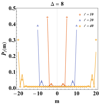
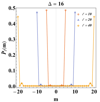
Figure 7: PDF of the staggered subsystem magnetization for several subsystem sizes $\ell$ evaluated in the thermal state $\rho_{\rm SS}$ with inverse effective temperature $\beta_{\rm eff}$ fixed by the value of the energy in the initial Néel state; namely $\beta_{\rm eff}=1.241,\,0.789$ for $\Delta=8,\,16$. Symbols are exact numerical data, lines are the large-$\Delta$ expansion obtained by taking the Fourier transform of (B) and (50). The agreement at $\Delta=16$ is excellent.

In Fig. 7 we compare the PDF in the thermal state with inverse temperature fixed by the condition $\langle{\rm GS}_{\infty}^{+}|H_{\Delta}|{\rm GS}_{\infty}^{+}\rangle={\rm Tr}\left[\rho_{\rm SS}H_{\Delta}\right]$ with the results of the large-$\Delta$/low density expansion. As expected, the agreement is increasingly better for larger values of the anisotropy.

References

- (1) T. Langen, R. Geiger and J. Schmiedmayer, Ultracold Atoms Out of Equilibrium, Ann. Rev. Cond. Matt. Phys. 6, 201 (2015).
- (2) E. Altman, Nonequilibrium quantum dynamics in ultracold quantum gases in Strongly Interacting Quantum Systems out of Equilibrium: Lecture Notes of the Les Houches Summer School, eds T. Giamarchi, A.J. Millis, O. Parcollet, H. Saleur and L.F. Cugliandolo, 99 (2012).
- (3) T. Kinoshita, T. Wenger, D. S. Weiss, A quantum Newton’s cradle, Nature 440, 900 (2006).
- (4) M. Greiner, O. Mandel, T.W. Hänsch, and I. Bloch, Collapse and revival of the matter wave field of a Bose-Einstein condensate, Nature 419, 51-54 (2002).
- (5) L. Hackermuller, U. Schneider, M. Moreno-Cardoner, T. Kitagawa, S. Will, T. Best, E. Demler, E. Altman, I. Bloch and B. Paredes, Anomalous Expansion of Attractively Interacting Fermionic Atoms in an Optical Lattice, Science 327, 1621 (2010).
- (6) S. Trotzky Y.-A. Chen, A. Flesch, I. P. McCulloch, U. Schollwöck, J. Eisert, and I. Bloch, Probing the relaxation towards equilibrium in an isolated strongly correlated 1D Bose gas, Nature Phys. 8, 325 (2012).
- (7) U. Schneider, L. Hackermüller, J. P. Ronzheimer, S. Will, S. Braun, T. Best, I. Bloch, E. Demler, S. Mandt, D. Rasch, and A. Rosch, Fermionic transport and out-of-equilibrium dynamics in a homogeneous Hubbard model with ultracold atoms, Nature Phys. 8, 213 (2012).
- (8) M. Cheneau, P. Barmettler, D. Poletti, M. Endres, P. Schauss, T. Fukuhara, C. Gross, I. Bloch, C. Kollath, and S. Kuhr, Light-cone-like spreading of correlations in a quantum many-body system, Nature 481, 484 (2012).
- (9) T. Langen, R. Geiger, M. Kuhnert, B. Rauer, and J. Schmiedmayer, Local emergence of thermal correlations in an isolated quantum many-body system, Nature Phys. 9, 640 (2013).
- (10) F. Meinert, M.J. Mark, E. Kirilov, K. Lauber, P. Weinmann, A.J. Daley, and H.-C. Nägerl, Quantum Quench in an Atomic One-Dimensional Ising Chain, Phys. Rev. Lett. 111, 053003 (2013).
- (11) J.P. Ronzheimer, M. Schreiber, S. Braun, S.S. Hodgman, S. Langer, I.P. McCulloch, F. Heidrich-Meisner, I. Bloch and U. Schneider, Expansion dynamics of interacting bosons in homogeneous lattices in one and two dimensions, Phys. Rev. Lett. 110, 205301 (2013).
- (12) N. Navon, A.L. Gaunt, R.P. Smith and Z. Hadzibabic, Critical Dynamics of Spontaneous Symmetry Breaking in a Homogeneous Bose gas, Science 347, 167 (2015).
- (13) Y. Tang, W. Kao, K.-Y. Li, S. Seo, K. Mallayya, M. Rigol, S. Gopalakrishnan and B.L. Lev, Thermalization near integrability in dipolar quantum Newton’s cradle, Phys. Rev. X 8, 021030 (2018).
- (14) S. Hofferberth, I. Lesanovsky, T. Schumm, A. Imambekov, V. Gritsev, E. Demler, and J. Schmiedmayer, Probing quantum and thermal noise in an interacting many-body system, Nature Phys. 4, 489 (2008).
- (15) T. Kitagawa, S. Pielawa, A. Imambekov, J. Schmiedmayer, V. Gritsev, and E. Demler, Ramsey Interference in One-Dimensional Systems: The Full Distribution Function of Fringe Contrast as a Probe of Many-Body Dynamics, Phys. Rev. Lett. 104, 255302 (2010).
- (16) T. Kitagawa, A. Imambekov, J. Schmiedmayer, and E. Demler, The dynamics and prethermalization of one-dimensional quantum systems probed through the full distributions of quantum noise, New J. Phys. 13, 73018 (2011).
- (17) M. Gring, M. Kuhnert, T. Langen, T. Kitagawa, B. Rauer, M. Schreitl, I. Mazets, D. A. Smith, E. Demler, and J. Schmiedmayer, Relaxation and Prethermalization in an Isolated Quantum System, Science 337, 1318 (2012).
- (18) A. Mazurenko, C.S. Chiu, G. Ji, M.F. Parsons, M. Kanasz-Nagy, R. Schmidt, F. Grusdt, E. Demler, D. Greif and M. Greiner, Experimental realization of a long-range antiferromagnet in the Hubbard model with ultracold atoms, Nature 545, 462 (2017).
- (19) M. Först et al, Melting of Charge Stripes in Vibrationally Driven : Assessing the Respective Roles of Electronic and Lattice Order in Frustrated Superconductors, Phys. Rev. Lett. 112, 157002 (2014).
- (20) R. Mankowsky, M. Först and A. Cavalleri, Non-equilibrium control of complex solids by nonlinear phononics, Rep. Progr. Phy. 79 064503 (2016).
- (21) J. M. Deutsch, Quantum statistical mechanics in a closed system, Phys. Rev. A 43, 2046 (1991).
- (22) M. Srednicki, Chaos and quantum thermalization, Phys. Rev. E50, 888 (1994).
- (23) M. Rigol, V. Dunjko, and M. Olshanii, Thermalization and its mechanism for generic isolated quantum systems, Nature 452, 854 (2008).
- (24) M. Rigol, V. Dunjko, V. Yurovsky, and M. Olshanii, Relaxation in a Completely Integrable Many-Body Quantum System: An Ab Initio Study of the Dynamics of the Highly Excited States of 1D Lattice Hard-Core Bosons, Phys. Rev. Lett. 98, 50405 (2007).
- (25) A. C. Cassidy, C. W. Clark, and M. Rigol, Generalized Thermalization in an Integrable Lattice System, Phys. Rev. Lett. 106, 140405 (2011).
- (26) J.-S. Caux and F.H.L. Essler, Time Evolution of Local Observables After Quenching to an Integrable Model, Phys. Rev. Lett. 110, 257203 (2013).
- (27) E. Ilievski, J. De Nardis, B. Wouters, J.-S. Caux, F.H.L. Essler, T. Prosen, Complete Generalized Gibbs Ensemble in an interacting Theory, Phys. Rev. Lett. 115, 157201 (2015).
- (28) B. Pozsgay, The generalized Gibbs ensemble for Heisenberg spin chains, J. Stat. Mech. P07003 (2013).
- (29) M. Fagotti and F.H.L. Essler, Stationary behaviour of observables after a quantum quench in the spin-1/2 Heisenberg XXZ chain, J. Stat. Mech. P07012 (2013).
- (30) M, Fagotti, M, Collura, F.H.L. Essler, and P. Calabrese, Relaxation after quantum quenches in the spin-1/2 Heisenberg XXZ chain, Phys. Rev. B 89, 125101 (2014).
- (31) B. Wouters, J. De Nardis, M. Brockmann, D. Fioretto, M. Rigol, J.-S. Caux, Quenching the Anisotropic Heisenberg Chain: Exact Solution and Generalized Gibbs Ensemble Predictions, Phys. Rev. Lett. 113, 117202 (2014).
- (32) M. Brockmann, B. Wouters, D. Fioretto, J. De Nardis, R. Vlijm and J.-S. Caux, Quench action approach for releasing the Néel state into the spin-1/2 XXZ chain, Stat. Mech. P12009 (2014).
- (33) B. Pozsgay, M. Mestyán, M.A. Werner, M. Kormos, G. Zaránd, and G. Takács, Correlations after Quantum Quenches in the XXZ Spin Chain: Failure of the Generalized Gibbs Ensemble, Phys. Rev. Lett. 113, 117203 (2014).
- (34) M. Mestyán, B. Pozsgay, G. Takács, and M.A. Werner, Quenching the XXZ spin chain: quench action approach versus generalized Gibbs ensemble, J. Stat. Mech. P04001 (2015).
- (35) E. Ilievski, E. Quinn, J. De Nardis and M. Brockmann, String-charge duality in integrable lattice models, J. Stat. Mech. 063101 (2016).
- (36) G. Vidal, Classical Simulation of Infinite-Size Quantum Lattice Systems in One Spatial Dimension, Phys. Rev. Lett. 98, 070201 (2007).
- (37) R. Orús and G. Vidal, Infinite time-evolving block decimation algorithm beyond unitary evolution, Phys. Rev. B 78, 155117 (2008).
- (38) P. Barmettler, M. Punk, V. Gritsev, E. Demler, and E. Altman, Relaxation of antiferromagnetic order in spin-1/2 chains following a quantum quench, Phys. Rev. Lett. 102, 130603 (2009).
- (39) P. Barmettler, M. Punk, V. Gritsev, E. Demler, and E. Altman, Quantum quenches in the anisotropic spin-1/2 Heisenberg chain: different approaches to many-body dynamics far from equilibrium, New J. Phys. 12, 055017 (2010).
- (40) S. Sotiriadis and J. Cardy, Quantum quench in interacting field theory: A self-consistent approximation, Phys. Rev. B 81, 134305 (2010).
- (41) Y.D. van Nieuwkerk and F.H.L. Essler, Self-consistent time-dependent harmonic approximation for the Sine-Gordon model out of equilibrium, arXiv:1812.06690.
- (42) S. Groha, F.H.L. Essler and P. Calabrese, Full Counting Statistics in the Transverse Field Ising Chain, SciPost Phys. 4, 043 (2018).
- (43) F.H.L. Essler and R.M. Konik, Finite Temperature Dynamical Correlations in Massive Integrable Quantum Field Theories, J. Stat. Mech. P09018 (2009).
- (44) A.J.A. James, F.H.L. Essler and R.M. Konik, Finite Temperature Dynamical Structure Factor of Alternating Heisenberg Chains, Phys. Rev. B78, 094411 (2008).
- (45) W.D. Goetze, U. Karahasanovic and F.H.L. Essler, Low-Temperature Dynamical Structure Factor of the Two-Leg Spin-1/2 Heisenberg Ladder, Phys. Rev. B82, 104417 (2010).
- (46) B. Pozsgay and G. Takacs, Form factor expansion for thermal correlators, J. Stat. Mech. P11012 (2010).
- (47) I.M. Szecsenyi and G. Takacs, Spectral expansion for finite temperature two-point functions and clustering, J. Stat. Mech.P12002 (2012).
- (48) P. Calabrese, F.H.L. Essler, and M. Fagotti, Quantum Quench in the Transverse-Field Ising Chain, Phys. Rev. Lett. 106, 227203 (2011).
- (49) P. Calabrese, F.H.L. Essler, and M. Fagotti, Quantum quench in the transverse field Ising chain: I. Time evolution of order parameter correlators. J. Stat. Mech. P07016 (2012).
- (50) D. Schuricht and F.H.L. Essler, Dynamics in the Ising field theory after a quantum quench, J. Stat. Mech., P04017 (2012).
- (51) B. Bertini, D. Schuricht, and F.H.L. Essler, Quantum quench in the sine-Gordon model, J. Stat. Mech. P10035 (2014).
- (52) A. H. MacDonald, S. M. Girvin, D. Yoshioka, Phys. Rev. B 37, 16 (1988).
- (53) L. Bonnes, F.H.L. Essler and A. Läuchli, “Light-Cone” Dynamics After Quantum Quenches in Spin Chains, Phys. Rev. Lett. 113, 187203 (2014).
- (54) B. Bertini, F.H.L. Essler, S. Groha, N.J. Robinson, Thermalization and light cones in a model with weak integrability breaking, Phys. Rev. B 94, 245117 (2016).
- (55) M. Fagotti and P. Calabrese, Entanglement entropy of two disjoint blocks in XY chains, J. Stat. Mech. P04016 (2010).