How to correctly quantify neuronal phase-response curves from noisy recordings

Abstract

At the level of individual neurons, various coding properties can be inferred from the input-output relationship of a cell. For small inputs, this relation is captured by the phase-response curve (PRC), which measures the effect of a small perturbation on the timing of the subsequent spike. Experimentally, however, an accurate experimental estimation of PRCs is challenging. Despite elaborate measurement efforts, experimental PRC estimates often cannot be related to those from modeling studies. In particular, experimental PRCs rarely resemble the generic PRC expected close to spike initiation, which is indicative of the underlying spike-onset bifurcation. Here, we show for conductance-based model neurons that the correspondence between theoretical and measured phase-response curve is lost when the stimuli used for the estimation are too large. In this case, the derived phase-response curve is distorted beyond recognition and takes on a generic shape that reflects the measurement protocol, but not the real neuronal dynamics. We discuss how to identify appropriate stimulus strengths for perturbation and noise-stimulation methods, which permit to estimate PRCs that reliably reflect the spike-onset bifurcation – a task that is particularly difficult if a lower bound for the stimulus amplitude is dictated by prominent intrinsic neuronal noise.

I Introduction

Neuronal dynamics are commonly studied based on the response of a neuron to specific stimuli. The spiking in response to post-synaptic currents or temporally structured inputs, for example, often serves as a first indication for the neuronal code. Constraining the response to weak stimuli, a neuron’s spiking dynamics can be captured by the so-called phase-response curve (PRC). The PRC relates the timing of a short stimulus pulse to the consequential advance or delay of the next spike. As a well-defined theoretical quantity, the PRC is also experimentally accessible. PRCs are valuable to decipher single-cell dynamics, such as the neuronal response to a particular input shape, e.g. synaptic inputs (Reyes and Fetz, 1993a; Netoff et al., 2005b) or noise (Ermentrout et al., 2008), as well as the locking time to a time-dependent stimulus (Kuramoto, 1984; Achuthan et al., 2011). Beyond single cells, PRCs are often used to predict how neurons behave when weakly connected, informing about network dynamics and, in particular, their synchronization state (Van Vreeswijk et al., 1994; Hansel et al., 1995; Ermentrout, 1996; Galán et al., 2005; Teramae and Fukai, 2008; Smeal et al., 2010). Beyond the neurosciences, the PRC is used for various other biological oscillations such as cardiac pacemakers or circadian rhythms (Guevara et al., 1981; Minors et al., 1991).

As we show in the following, suboptimal measurement protocols yield PRCs that do not accurately reflect neuronal dynamics. In order to estimate PRCs experimentally, neuronal spiking is perturbed by an experimentally known stimulus. The amplitude range of this stimulus is bounded from below and from above: On one hand, the experimental stimulus has to be chosen large enough to overcome intrinsic noise, which perturbs spiking in addition to the stimulus (Manwani and Koch, 1999). On the other hand, the stimulus has to be weak enough such that the PRC is a valid description of the dynamics: Stimulus amplitudes have to be sufficiently small to allow the dynamics to relax back to the limit cycle within one period, because the PRC assumes independence of subsequent spikes. As a rule of thumb, the larger the intrinsic noise, the more restricted the range of acceptable stimulation amplitudes.

Relatively strong intrinsic noise is, for example, typical for cortical and hippocampal neurons, which often show notable spike jitter even for constant step current stimuli. We show that the consequential variability of the phase response observed experimentally can impair PRC measurements (Wang et al., 2013; Stiefel and Ermentrout, 2016). This was not observed previously because the methods for quantification of PRCs were typically illustrated with neurons showing only low levels of intrinsic noise, and thus stable firing rates (for a review see Torben-Nielsen et al. (2010a)).

Here, we address the identification of spike-onset bifurcations from PRC measurements. Spiking in neurons can be classified into four basic mechanisms of spike initiation (Izhikevich, 2007). The corresponding spike-onset bifurcations give rise to distinguishable, generic PRCs that reflect neuronal dynamics at spike onset (Ermentrout, 1996; Izhikevich, 2000). We show that the mapping between PRC and spike-onset bifurcation is lost when the measurement stimulus is not chosen appropriately. In this case, the PRC shape becomes independent of the neuron’s dynamics, and only reflects the measurement protocol.

In the following, we compare the measurement accuracy of three different PRC methods faced with strong intrinsic noise. While Torben-Nielsen et al. (2010a) have previously considered different methods under relatively benign conditions, we are interested in extreme conditions with large stimuli or large intrinsic noise levels. Exploring the border where a PRC estimation becomes invalid allows us to delineate the range of experimental conditions under which PRC measurements can be expected to actually yield information on neuronal dynamics.

II Methods

II.1 Models

PRCs were measured for conductance-based neuron models with three different spike onset bifurcations, for details see Appendix. Of the four possible limit cycle bifurcations for spike initiation (Izhikevich, 2007), we have chosen those that result in biologically realistic all-or-none spikes with finite voltage amplitude at spike onset: the subcritical Hopf bifurcation, the saddle-node on invariant cycle (SNIC) bifurcation and the saddle-homoclinic orbit (HOM) bifurcation. The level of the intrinsic noise was set by the standard deviation of an additive zero-mean white-noise current, see Appendix.

II.2 Phase-response curve

For a regular spiking conductance-based neuron model with baseline period $T$ (firing rate $f=1/T$), weakly perturbed spiking can be described by an input-output equivalent phase oscillator,

$$\dot{\varphi}=1+Z(t)s(t),$$ (1)

with $Z$ as PRC, and a time-dependent stimulus $s(t)$. In response to the stimulus $s(t)$, the spike at $t=t_{i+1}$ following the spike $t=t_{i}$ is advanced or delayed according to the phase deviation

$$\Delta\varphi=\int_{t=t_{i}}^{t_{i}+T}Z(t)s(t)\textrm{d}t.$$ (2)

II.3 Theoretical estimation of the PRC

For mathematical neuron models, the PRC can be gained by numerical integration, for a review see Govaerts and Sautois (2006). For a conductance based neuron model with equation $\dot{x}=F(x)$, the linearized dynamics on the limit cycle are given as $\dot{x}=Jx$ with the Jacobian $J=\frac{\partial F}{\partial x}$. The corresponding adjoint equation is $\dot{y}=-J^{\mathrm{T}}y$. As these dynamics are unstable, backward integration in time along the limit cycle leads to a stable solution $y$, whose first entry corresponds to the voltage PRC (Ermentrout and Kopell, 1991; Ermentrout, 1996). We use this method to derive the “true” PRC for the models. The comparison of theoretical PRC and PRCs estimated with experimentally-inspired methods allows us to suggest the appropriate input strength, as well as a reasonable noise level, both of which can be employed in biological experiments to prevent false PRC measures as mentioned in the introduction.

II.4 Experimental methods of PRC measurements

We consider three different methods for PRC estimation. The estimation analyzes spike timing in response to a known stimulus. For the first method, neuronal spiking is perturbed by a sequence of short current pulses, the other two method use a noise stimulus. In addition, the neuron is stimulated with a DC current that ensures repetitive spiking; we choose a baseline firing rate of 10Hz (i.e., with period $T$ = 100ms). The simulation duration is sufficient to record about 500 perturbed spikes, for details see Appendix.

For two consecutive spikes at time $t=t_{i}$ and $t=t_{i+1}$, the actual interspike interval duration is $\textrm{ISI}_{i}=t_{i+1}-t_{i}$. For the phase response, we normalize the time during the unperturbed period $T$ to a phase variable $\varphi$ that ranges from zero to one. For a perturbed interspike interval, the change in duration is captured by the phase deviation, $\Delta\varphi_{i}=1-(t_{i+1}-t_{i})/T$, which is positive for spike advances, and negative for phase delays.

For plotting purposes, the PRCs are commonly fitted either with polynomial functions, e.g., Netoff et al. (2005a), or with Fourier series consisting of a low number of Fourier coefficient, e.g., Galán et al. (2005). As we are here also interested in PRCs with steep components (such as the PRC of the HOM model in Figure 2a), we choose a Fourier series of order five (i.e., with 11 Fourier components) to fit our PRC estimates,

$$Z(\varphi)=a_{0}+\sum_{j=1}^{5}\left(a_{j}\cos(2\pi j\varphi)+b_{j}\sin(2\pi j\varphi)\right),$$ (3)

with Fourier coefficients ${a_{0},a_{1},...a_{5},b_{1},...,b_{5}}$. Using the same number of Fourier components for all PRC estimates facilitates the comparison of different methods.

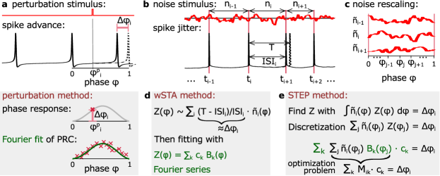
Figure 1: Experimental methods for PRC measurements. a: Individual time-point perturbation. The phase deviation $\Delta\varphi$, resulting from stimulation with a short current pulse, is plotted against the timing of the current pulse, and fitted by a curve. b: Time-continuous noise stimulation. Spikes are jittered due to a continuous noise-stimulation. c: Noise is rescaled to the phase variable. d: The wSTA method estimates the PRC via a weighted spike-triggered average. e: The STEP method relies on an error minimization of the input-and-PRC-based prediction of spike jitter.

II.4.1 PRC estimation based on individual-timepoint perturbation

For the PRC estimation based on individual-timepoint perturbations, the repetitively spiking neuron is stimulated with delta current pulses of a specific amplitude. The perturbation method was chosen for most experimentally measured PRCs (Reyes and Fetz, 1993b, a; Goldberg et al., 2007; Tsubo et al., 2007; Wang et al., 2013), as it is intuitive and easily analyzed. Here, the interval between two successive pulses is chosen randomly between 150ms and 250ms, such that most perturbations occur as single events in every second interspike interval. This ensures the independence of subsequent perturbations, allowing the dynamics a whole period to relax.

The analysis evaluates interspike intervals in which a current pulse occurs. The timing of the perturbation is related to the resulting phase deviation, compare Figure 1a. Given a current pulse at $t=t_{p}$ between two consecutive spikes at $t=t_{i}$ and $t=t_{i+1}$, the PRC relates the phase deviation, $\Delta\varphi_{i}=1-(t_{i+1}-t_{i})/T$, to the phase at which the current pulse occurred, $\varphi^{p}_{i}=(t_{p}-t_{i})/T$ (Rinzel and Ermentrout, 1989). An estimate of the PRC in units of phase deviation is gained by plotting the phase deviation against the perturbation phase. More precisely, each point of this graph corresponds to a stochastic drawing from the underlying PRC. In order to get the PRC in response to current perturbations, the PRC in units of phase deviation is divided by the amplitude of the perturbation stimulus.

For neurons with intrinsic noise, even weak noise perturbs the raw data so strongly that the PRC shape can often not be identified by naked eye. To fit a curve to the raw PRC data, we here use Galán’s method (Galán et al., 2005; Netoff et al., 2011), for which the Fourier components of Eq. (3) are given for a set of $N$ perturbed spikes as

$$a_{0}=\frac{1}{N}\sum_{i=1}^{N}\Delta\varphi_{i},\quad a_{j}=\frac{1}{N}\sum_{i=1}^{N}\Delta\varphi_{i}\cos(2\pi j\varphi^{p}_{i}),$$

$$\quad b_{j}=\frac{1}{N}\sum_{i=1}^{N}\Delta\varphi_{i}\sin(2\pi j\varphi^{p}_{i}).$$

II.4.2 PRC estimation based on time-continuous noise stimulation

For the PRC estimation based on noise-stimulation, the repetitively spiking neuron is stimulated with a zero-mean noise stimulus. We use a colored noise current with time resolution of $dt=10\mu\textrm{s}$, resulting from filtering a white noise signal with a cut-off frequency of 1000Hz.

For each spike, the recorded phase deviation $\Delta\varphi_{i}$ is related to the noise snippet $n_{i}$ that corresponds to the preceding interspike interval, see Figure 1b. The duration of the noise snippet $n_{i}(t)$ is rescaled to the phase variable, resulting in a phase-dependent noise snippet $\tilde{n}_{i}(\varphi)$, see Figure 1c.

To estimate PRCs from the noise-stimulated spike trains, we use the weighted Spike-Triggered Average (wSTA) introduced by Ota et al. (2009) and the STandardized Error Prediction (STEP) method introduced by Torben-Nielsen et al. (2010b).

The wSTA method sums over the phase-dependent noise snippets, while weighting each noise snippet by a variant of the phase deviation $\bar{\Delta\varphi}=(T/(t_{i+1}-t_{i})-1)$, see Figure 1d. For the correct amplitude scaling, the result is then divided by the variance of the noise input.

The STEP method optimizes the PRC shape to predict the phase deviation caused by the noise input since the previous spike. The idea takes advantage of Eq. (2), which predicts the phase deviation resulting from the stimulus $s(t)=n_{i}(t)$. Both the PRC and the phase-dependent noise snippets are discretized by a temporal binning with 200 phase bins. This allows to replace the integration in Eq. (2) by a simple sum of the PRC and the phase-dependent snippet $\tilde{n}_{i}$ (Figure 1e). To create an optimization matrix $\mathbf{{M}}$, the binned versions of noise and base functions are multiplied (Figure 1e). Linear least square optimization (here we used the python function numpy.linalg.lstsq()) allows to find the Fourier coefficients that, when multiplied by the matrix $\mathbf{{M}}$, best recover the phase deviations extracted from the raw data of spike times.

An advantage of the perturbation method and the wSTA method compared to the STEP method is that the PRC estimates can be implemented as an ongoing process that continuously allows to add new data as it is available. In contrast, the STEP method, and similar methods that rely on spike prediction error minimization, require a set of noise/spike-timing pairs of a fixed size, and, at least in current implementations, the optimization has to be redone when new data is collected.

III Results

In order to measure PRCs experimentally from repetitively firing neurons, the spike times are perturbed by an additional stimulus consisting of either a noise current or short pulse-like perturbations. Under the assumption that the stimulus has to be weak, intrinsic noise in real neurons makes the appropriate scaling of the stimulus amplitude a non-trivial problem (Netoff et al., 2011). The stimulus has to be large enough to stand out against the intrinsic noise, yet also small enough to prevent the instantaneous induction of spikes.

While most previous studies focus on the PRC shape, and neglect the PRC amplitude, we here also evaluate the PRC amplitude. The PRC amplitude is essential for a quantitative comparison of measurements, as it scales quantities derived from the PRC such as the synchronization range or the transition time until locking is established.

III.1 PRC estimates with perturbations or noise stimuli

Figure 2a-b shows PRC estimates for models without intrinsic noise with three different spike generation mechanisms (top to bottom), using three different methods (left to right: perturbation method, wSTA method and STEP method), see Methods for details. For comparison, each small panel depicts the theoretical PRC (brown) and PRCs estimated from spiking in response to different stimulus strengths (color-coded from green to violet). While all three methods estimate the shape of the PRC with similar quality, the STEP method has a tendency to overestimate the amplitude of the PRC, which is not observed for the perturbation method and the wSTA method.

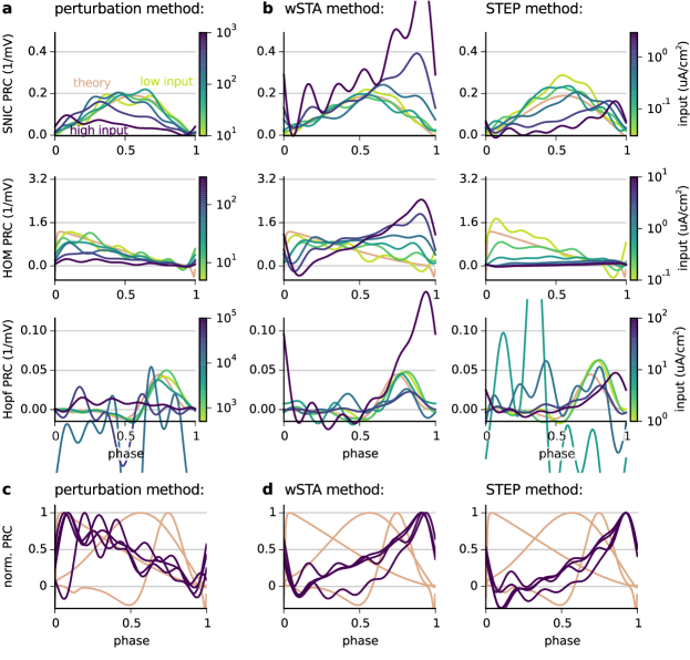
Figure 2: Comparing PRC measurements for three spike generation mechanism (input strength is color-coded from green to violet). The smooth theoretical PRC is depicted in brown. a: PRCs measured with the perturbation method. b: PRCs measured with wSTA and STEP method. c-d: Comparison of different dynamical classes at highest stimulus amplitude from (a-b).

For the Hopf model, the PRC derived with the wSTA method seems reasonable. In contrast, the perturbation method and the STEP method both lead to strongly wiggling PRCs for intermediate stimulus amplitudes, see Figure 2a-b. The wiggling PRCs occur for stimulus amplitudes for which the model becomes extremely sensitive to inputs (the CV shows a maximum in response to these noise strength). As a side-note, this behavior was also observed for another model with subcritical Hopf bifurcation at spike onset, the original Hodgkin-Huxley model (Hodgkin and Huxley, 1952).

III.2 Stimulus amplitude dependence

The range of stimulus amplitudes in Figure 2a-b is chosen to illustrate the transition from good to bad PRC estimates. Because the models lack intrinsic noise, the theoretical curve (brown) is best fitted by the PRC with the lowest input strength (green), and reasonable fits are derived for a range of small stimulus levels. The correspondence between theoretical and estimated PRC is lost for intermediate stimulus levels, and the estimated PRC approaches a characteristic shape for large stimulus levels. Figure 2c-d summarizes the PRC estimates corresponding to the largest stimulus strength (the violet curves from Figure 2a-b). For all methods, these PRCs have a characteristic shape that is hardly distinguishable for different spike generation mechanisms, and thus the PRC is not informative about neuronal dynamics. With such a large input, the drive is too strong to estimate meaningful PRCs, and we call this regime in the following the overdriven regime.

III.3 Shape of overdriven PRCs

The stereotypical PRC shape in the overdriven regime (Figure 2c-d) shows a linear relation for intermediate phases, with a steep connection around phase zero that is enforced by the periodicity of the Fourier-series fit. The linear decrease/increase observed for the perturbation and noise-stimulation methods, respectively, results from instantaneous spikes in response to large perturbations in the stimulus.

For the perturbation method (Figure 2c), the instantaneous initiation of spikes results in larger phase advances for earlier perturbation phases, which directly translate into a linear decrease, see Figure 3a. For the overdriven PRC in units of phase deviation, the slope of the PRC is minus one, which has been termed the causality limit (Netoff et al., 2011) or causal limit (Wang et al., 2013).

For the noise methods, spikes are mostly induced by spontaneous, large deviations of the noise stimulus. As a result, the noise snippets show an exceptionally large amplitude right before the spike, i.e., close to phase one (Figure 3b). Adding those snippets up in a weighted spike-triggered average, transfers the large amplitude close to phase one to the PRC, which eventually results in a linearly increasing overdriven PRC (Figure 2d). Also for the STEP method, this temporal stretching induces a bias. As the neuron seems to react particularly sensitively to inputs right before the spike, it again induces a large PRC amplitude close to a phase equal to one.

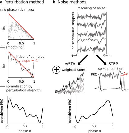
Figure 3: Perturbation and noise-stimulation methods lead to different but stereotypic PRCs. a: For the perturbation method, the overdriven PRC result from the advance of the spike to the time point of the perturbation. b: The shape of the overdriven PRC results for the noise stimulation methods from temporally stretched noise snippets with an elevation before the following spike.

How easily an overdriven PRC can be confounded with a real PRC depends on the combination of true PRC and estimation method. For example, the overdriven PRC of the perturbation method can be easily mistaken for the PRC of a HOM spike generation, while the overdriven PRCs of the noise methods might be mistaken for the PRC of a Hopf spike generation.

III.4 Dependence on internal noise

When measuring PRCs in biological neurons, recordings will be perturbed by various intrinsic noise sources including ion channel noise and recording noise (Manwani and Koch, 1999). We next test the stability of PRC estimates for models implementing intrinsic noise with a strong, yet biologically realistic standard deviation, see Appendix for details.

With intrinsic noise, we observe an intermediate stimulus strength that leads to optimal PRC estimates (third column in Figure 4). For small stimulus amplitudes, the stimulus’ effect on spike timing is veiled by the intrinsic noise, which jitters the spikes more than the stimulus. This results in PRC estimates hardly above noise level, and the quality of the PRC estimates augments with increasing stimulus amplitude (Figure 4, from the first to the third column), while the estimation error decreases. Further increase in the stimulus amplitude leads to the overdriven regime, first indications of which are visible in the forth column of Figure 4; the shift in the peak (compare Figure 2a-b) will continue with increasing stimulus amplitude until the linear PRC is fully established. The error amplitude continues to decrease with stimulus amplitude in the overdriven regime (data not shown). Indeed, the overdriven regime implies a stark, unrealistic reduction in both error types, which shows in published experimental results (Reyes and Fetz, 1993a, b; Goldberg et al., 2007).

A comparison between two intrinsic noise levels demonstrates that, as expected, larger intrinsic noise results in larger errors and increases the minimal possible stimulus amplitude (Figure 4, stronger noise in bottom panels compared to top).

Figure 4: Perturbation and noise-stimulation methods perform similar under high intrinsic noise levels. The PRC estimation is exemplified with the SNIC model, theoretical PRC in brown; the intrinsic noise is adapted to a baseline coefficient of variation (CV) of 0.2 and 0.3, respectively. For the bottom traces, the PRC estimation directly reaches the overdriven regime once the stimulus amplitude is large enough to counter the intrinsic noise, not allowing for an intermediate, appropriate range of stimulus amplitudes. Bootstrapping of the data results in standard deviation errors for the PRC (transparent colored area) and for the zero-PRC background (grey area), see Appendix.

Interestingly, all PRC estimation methods result in a comparable PRC quality (similar shape, amplitude and error levels). This result contrasts previous suggestions that the noise-stimulation method should be less disturbed by intrinsic noise compared to the perturbation method (Izhikevich, 2007; Netoff et al., 2011). In Figure 4, even strong intrinsic noise that induces a baseline coefficient of variation (CV) of about 0.2 leads to similar PRC estimates for all methods, while small differences might be observed for slightly higher noise levels with a CV of about 0.3, which is close to the maximum intrinsic noise that still allows to derive PRCs.

III.5 Practical scaling of the input signal

When measuring PRCs from an experimentally recorded neuron, what is the correct amplitude of the signal? Our results suggest that the stimulus in addition to the DC current (i.e., perturbation or noise) should increase the firing rate by less than 10% above baseline (i.e., when stimulated only with the DC current). The increase in firing rate results from the positive mean value of the PRC observed for most neurons, which predicts that positive inputs will, on average, advance spikes to earlier phases. The stronger the input amplitude, the larger the increase in firing rate. In particular, our data suggests that the overdriven regime correlates with a relative increase in firing rate exceeding 10%.

So far, common practice recommended to aim for noise stimuli that are sufficiently large to induce voltage deflections on the order of 1mV, visible by bare eye (Netoff et al., 2011). Yet, experimental results complying with these recommendations already show indications of the overdriven regime (Reyes and Fetz, 1993b; Goldberg et al., 2007). Also in our simulations, we found that at least for neurons with relatively high intrinsic noise, this best practice overestimates the required stimulus amplitude and thus results in overdriven PRCs.

To bound the stimulus amplitude, one could consider the increase in spike jitter due to the stimulation, as measured by the coefficient of variation (CV). In our numerical simulations, the resulting CV, can be relatively large (up to a CV of 1) without reaching the overdriven regime, depending on the neuronal dynamics. Accordingly, we found absolute CV values to be of minor help to establish the correct stimulus amplitude.

To summarize, a correct stimulus amplitude is indicated by a relative increase in firing rate by maximally 10% when adding the stimulus to the DC current. In contrast to the common assumption that the perturbing stimulus should be clearly identifiable against the intrinsic noise, the stimulus signal is in this case not visible by eye in the interspike voltage trace.

III.6 Checking the PRC estimate

The reporting of overdriven PRCs is undesirable, because they can severely misrepresent neuronal dynamics. To check the quality of PRC estimates, we propose three post-experimental analyses.

As mentioned above, one hallmark of the overdriven regime is an unrealistically low level of estimation errors, see Sect. III.4. Thus, reported PRCs should always be complemented by meaningful error bars, like those based on bootstrapping (described in the Appendix).

The recording of PRC data for multiple stimulus amplitudes provides a good test against overdriven PRCs for all estimation methods. For the perturbation method, this was previously recommended to identify stimuli that are too weak (Achuthan et al., 2011). We argue that after normalization with the stimulus strength, the amplitude of all PRC estimates with appropriate stimulus strength is comparable, while stimuli with too large an amplitude deviate and show a larger (wSTA) or smaller (STEP and perturbations) PRC amplitude. These size effects are easily singled out in recordings, in contrast to the above described alterations in PRC shape, which could be confused with the unknown, actual PRC shape as described in Sect. III.3. Recording multiple stimulus amplitudes thus helps to spot overdriven PRCs, yet at the cost of a prolongation of the total recording duration.

The noise methods provide a clear hallmark of overdriven PRCs without prolongating the recording duration when the same set of recorded spikes is evaluated with the wSTA as well as the STEP method. As can be seen in Figure 2b, both noise-stimulus methods yield similar PRC amplitudes as long as the input strength is appropriate. Yet, the effect of overdriven stimulation on the PRC amplitude is opposite for both methods. We thus propose to estimate PRCs from the same data via STEP and wSTA methods. A comparison of their respective amplitudes allows one to distinguish between valid and overdriven PRC measurements: Only if the corresponding PRCs are of similar amplitude, the measurement was performed with an appropriate input strength. If the estimated PRCs differ considerably in their (mean) amplitude, the measurement was most likely overdriven. This test can also be applied to existing data, as it is based on the same experimental recording being analyzed in two different ways.

IV Discussion

Neuronal phase-response curves have been measured for over twenty years (Reyes and Fetz, 1993a, b). PRCs are valuable to analyze neuronal dynamics, and can be used to predict synchronization and locking behavior of the neuron. We report pitfalls of experimental PRC measurements by comparing theoretical PRCs with PRCs estimated based on simulated spike trains. We find that reliable PRC estimates require an intermediate stimulus amplitude, sufficiently high to overcome intrinsic noise, but not too high to infringe fundamental PRC assumptions. As a result of the analysis, we propose to use stimulus amplitudes that change the firing rate by not more than 10% and that do not visibly impair the spike train. Stimulus amplitudes that are too large result in overdriven PRCs. Mild cases of overdriven PRCs are marked by a linear increase or decrease with reduced PRC error at low or high phases, respectively. Comparable hallmarks can be observed in previous experimental PRC measurements (Reyes and Fetz, 1993a, b; Goldberg et al., 2007; Farries and Wilson, 2012a, b; Wang et al., 2013). Even for mildly overdriven PRC estimates, information about neuronal dynamics may be occluded and conclusions based on these PRCs should be derived with care.

While experimental studies often refer to their estimated PRCs as “finite” PRCs, due to the finite, i.e., non-zero, stimulus amplitude of the experimental set-up, we here show that the distinction between “finite” PRC and the theoretical “infinitesimal” PRC is not supported by our results. We find that PRCs estimated with finite stimulus amplitude either fit the “infinitesimal” PRC, or they are not informative about neuronal dynamics: For stimuli that are too small, PRCs estimates are below noise level, and for stimuli that are too large, the PRCs approach a method-specific, generic shape that depicts the neuron misleadingly as a simplistic response machine. The transition from PRCs hardly above noise level, to PRCs with clear overdriven characteristics, is also observed in experimental studies with an increase in stimulus amplitude (Reyes and Fetz, 1993a; Netoff et al., 2005b). As these experimental examples show no clear PRC estimate that lies between intrinsic-noise-dominated and overdriven, the range of appropriate, intermediate stimulus amplitudes seems to be relatively small for the recorded hippocampal and cortical cells.

Here, we have compared PRC estimations for three methods. With optimal stimulus amplitude, all methods perform similarly (Torben-Nielsen et al., 2010a), and, contrary to previous assumptions (Izhikevich, 2007; Netoff et al., 2011), we show that even under noisy conditions, the perturbation method does not per se perform worse than the noise-stimulation methods. Yet, the prevention of overdriven PRCs is facilitated by the noise-stimulation methods compared to the perturbation method. Noise stimulation data allows to estimate the PRC based on the wSTA as well as the STEP method, and different PRC amplitudes in both measures provide a clear indication for overdriven PRCs.

Overdriven PRC estimates are a common problem in experimental studies. Farries and Wilson (2012a, b) report that even relatively large stimuli lead to reliable PRC estimates. Their solution to the problem of overdriven PRCs is a removal of the data points close to the causality limit. Others have related the causality limit to a biased sampling of phase (Phoka et al., 2010) or phase advance data (Wang et al., 2013). The authors propose methods to estimate the total distributions from the available, partial observations in order to get more realistic PRC estimates. While these approaches may help to extract more information from overdriven PRCs than the traditional analysis, they do not address the alterations in phase response due to the excessive stimulus amplitude discussed here.

The PRC amplitude is rarely reported in the literature, as many studies normalize the PRC amplitude arbitrarily, e.g., to one. This practice removes important information about the PRC: Not only is the amplitude required for any quantitative description of neuronal dynamics, it also provides a most valuable tool in testing for the overdriven regime. We stress that the correct amplitude scaling is as easily extracted from PRC data as the PRC shape itself.

Preventing overdriven PRCs becomes particularly relevant when measuring neurons with relatively high levels of intrinsic noise, such as cortical or hippocampal neurons, compared to neurons with stable repetitive firing. High levels of noise are also common when PRCs are estimated not for individual cells, but for whole brain areas. In these cases, attempted PRC measurements often suffer from exaggerated stimulus amplitudes in order to counter the intrinsic noise. In contrast, when measured with the appropriate stimulus amplitude, PRCs enrich our set of “diagnostic” tools to quantify neuronal dynamics.

Appendix

Conductance-based neuron models

Conductance-based neuron models were based on established models from the literature. The Hopf model was first described by Morris and Lecar; we use the version from Ermentrout and Terman (2010), p. 50-51. The SNIC and HOM models are versions of the Wang-Buzsaki model (Wang and Buzsáki, 1996). The membrane voltage $v$ of the models follows the dynamics

$$\frac{\mathrm{d}v}{\mathrm{d}t}=(I_{\mathrm{in}}+g_{\mathrm{L}}(E_{\mathrm{L}}-v)+I_{\mathrm{gates}})/C_{\mathrm{m}}.$$

The input current is the sum of a DC current, a time-dependent stimulus and an intrinsic noise $\xi$, $I_{\mathrm{in}}=I_{\mathrm{DC}}+s(t)+\sigma\xi$. For simulations without intrinsic noise, $\sigma=0$. The model parameters are summarized in Table 1.

Table 1: Parameters of the Hopf model and the SNIC model. The HOM model is equivalent to the SNIC model, but with $\phi=1.5$ and $I_{\mathrm{DC}}=0.166\mu$A/cm².

Parameter	Hopf	SNIC
$C_{\mathrm{m}}$	$20\mu$F/cm2	$1\mu$F/cm2
$E_{\mathrm{L}}$	$-60$mV	$-65$mV
$E_{\mathrm{Na}}$	$120$mV	$55$mV
$E_{\mathrm{K}}$	$-84$mV	$-90$mV
$g_{\mathrm{L}}$	$2\mathrm{mS/cm}^{2}$	$0.1\mathrm{mS/cm}^{2}$
$g_{\mathrm{Na}}$	$4.4\mathrm{mS/cm}^{2}$	$35\mathrm{mS/cm}^{2}$
$g_{\mathrm{K}}$	$8\mathrm{mS/cm}^{2}$	$9\mathrm{mS/cm}^{2}$
$I_{\mathrm{DC}}$	$90.76\mu$A/cm2	$0.212\mu$A/cm2
$\phi$	$0.04$	$1$

Gating for the Hopf model:

For the Hopf model,

$$I_{\mathrm{gates}}(v,n)=g_{\mathrm{Na}}m_{\infty}(v)(E_{\mathrm{Na}}-v)+g_{\mathrm{K}}n(E_{\mathrm{K}}-v).$$

The kinetics of the ion channel gating $n$ are given by

$$\frac{\mathrm{d}n}{\mathrm{d}t}=\phi\frac{n_{\infty}(v)-n}{\tau_{n}(v)},$$

with $\tau_{n}(v)={1\mathrm{ms}}/{\cosh\left((v/\mathrm{mV}-2)/60\right)}$. The ion channel activation curves are given as

$$m_{\infty}(v) = 0.5(1+\tanh((v/\mathrm{mV}-(-1.2))/18)),$$

$$n_{\infty}(v) = 0.5(1+\tanh((v/\mathrm{mV}-2)/30)).$$

Gating for the SNIC and HOM models:

For the SNIC model,

$$I_{\mathrm{gates}}(v,n,h)=g_{\mathrm{Na}}m_{\infty}(v)^{3}h(E_{\mathrm{Na}}-v)+g_{\mathrm{K}}n^{4}(E_{\mathrm{K}}-v).$$

The kinetics of the ion channel gating are given by

$$\frac{\mathrm{d}h}{\mathrm{d}t} = \phi(\alpha_{\textrm{h}}(v)(1-h)-\beta_{\textrm{h}}(v)h),$$

$$\frac{\mathrm{d}n}{\mathrm{d}t} = \phi(\alpha_{\textrm{n}}(v)(1-n)-\beta_{\textrm{n}}(v)n),$$

with

$$\alpha_{\textrm{h}}(v) = 0.07\exp(-\frac{v/\mathrm{mV}+58}{20})/\mathrm{ms},$$

$$\beta_{\textrm{h}}(v) = \frac{1}{1+\exp(-0.1v/\mathrm{mV}-2.8)}/\mathrm{ms},$$

$$\alpha_{\textrm{n}}(v) = \frac{0.01v/\mathrm{mV}+0.34}{1-\exp(-0.1v/\mathrm{mV}-3.4)}/\mathrm{ms},$$

$$\beta_{\textrm{n}}(v) = 0.125\exp(-\frac{v/\mathrm{mV}+44}{80})/\mathrm{ms},$$

The ion channel activation curve for the gating variable $m$ is given as

$$m_{\infty}(v) = \frac{\alpha_{\textrm{m}}(v)}{\alpha_{\textrm{m}}(v)+4\exp(-\frac{v/\mathrm{mV}+60}{18})},$$

$$\alpha_{\textrm{m}}(v) = \frac{0.1v/\mathrm{mV}+3.5}{1-\exp(-0.1v/\mathrm{mV}-3.5)}.$$

The HOM model is equivalent to the SNIC model, but with $\phi=1.5$ and $I_{\mathrm{in}}=0.166\mu$A/cm².

Conductance-based neuron models were simulated numerically with the simulation environment brian2 (Stimberg et al., 2014). To record 500 perturbed spikes, the recording duration is 50 seconds for the noise-stimulation methods, and 100 seconds for the perturbation method, where only every second spike is perturbed. We observed that the interspike interval depends on the time resolution $dt$ of the simulation. We have chosen $dt$ = 0.001ms for all models, to ensure that a three times smaller time step changed the deterministic interspike interval by less than 5%.

To investigate the tolerance of PRC measurements towards an unknown noise source, PRCs were in a second step measured for neuron models that included intrinsic noise, implemented as an additive zero-mean white-noise current (the brian2-implemented variable xi). The noise levels chosen in this study correspond to relatively strong intrinsic noise, with a phase noise of $\tilde{\sigma}=2\sqrt{\textrm{ms}}$ or $\tilde{\sigma}=3\sqrt{\textrm{ms}}$ standard deviation (Figure 4). The next section shows how to translate the phase noise into the standard deviation of the brian2-implemented noise variable xi. The chosen phase noise results in a CV of around 0.2 and 0.3, respectively, which is within a biologically realistic range.

As a side-note, while the stimulus amplitude appropriate for PRC estimation is larger for perturbations than for a noise stimulus, the latter induce more spike jitter (larger CVs) compared to the perturbations. It seems that as the perturbation is temporally precise, even small spike deviations are sufficient to estimate PRCs, while the continuous input delivered by the noise stimulus requires larger deviations to estimate the PRC, probably because every spike informs about the full phase range, instead of just one particular phase.

Adaptation of intrinsic noise levels for brian2 models

Comparable levels of the intrinsic noise between models can be ensured by identical noise levels in the phase reduction. This requires the following choice of the standard deviation of the intrinsic noise current, $\sigma$: The deterministic phase equation Eq. (1) is $\dot{\varphi}(t)=1+Zs(t)$ with current input $s(t)$ and PRC $Z$. With the intrinsic noise as input, and taking a temporal mean, we get $\dot{\varphi}(t)=1+\tilde{\sigma}\eta$, with the variance of the white noise $\eta$ as $\tilde{\sigma}^{2}=\sigma^{2}\int_{0}^{1}Z^{2}(\varphi)\mathrm{d}\varphi$. Setting the phase noise $\tilde{\sigma}$ to the same value in all models, we find the appropriate current noise strength as $\sigma=\tilde{\sigma}\frac{C_{\mathrm{m}}}{T}\left[\int_{0}^{1}Z^{2}(\varphi)\right]^{-0.5}\textrm{d}\varphi$, where $C_{\mathrm{m}}$ is the membrane capacitance of the model. For the simulations, we evaluate this formula with the theoretical PRCs gained from backwards integration of the adjoint equation as $Z$, see Section II.3.

Error estimation by bootstrapping

In order to evaluate the quality of the PRC, we use a bootstrap approach to estimate errors for the phase response curves. Two different kinds of phase-dependent errors are considered, the baseline error which results from PRC estimates on shuffled data, and the error on the PRC estimate.

In order to provide an error for the PRC, we repetitively estimate PRCs using only a restricted amount of spikes. We estimated PRCs in 100 repetitions from a set about 250 spikes, randomly chosen from the total set of about 500 perturbed spikes. The standard deviation of the 100 PRC estimates was used as PRC error.

In order to provide a baseline for the PRC estimate – above which a significant PRC should rise – we measure PRCs for random combinations of noise snippets and spike advances. We measure the PRC in 100 repetitions for a random permutation of the numbering $i$ of spike deviations $\{\Delta\varphi_{i}\}$, and calculate the standard deviation for the resulting 100 estimates. The mean of these estimates results in a PRC close to zero, such that the resulting standard deviation corresponds to the range within which a zero, i.e., non-significant PRC estimate is to be expected. This error around zero provides a lower bound to PRCs that are significantly different from zero.

Amplitude scaling for estimated phase-response curves

The appropriate unit for most experimentally derived PRCs is cm²/$\mu$A, which naturally arises for PRCs that measure the phase advance in response to a current, such as a noise stimulus or perturbation in $\mu$A/cm². For this study, however, we aim at comparing experimentally measured PRCs with theoretical PRCs. The theoretical PRCs gained from backwards integration of the adjoint equation have a unit of 1/mV, as they quantify the phase advance in response to a voltage perturbation in units of mV. For comparison, we transform the estimated PRCs into the units of the theoretical PRCs by dividing the current PRC by the membrane capacitance and the time window of the input, $Z(\Delta v)=Z(\Delta I)\;C_{\mathrm{m}}/\tilde{\tau}$, where $\tilde{\tau}$ is the temporal resolution of the measured PRC. $\tilde{\tau}$ corresponds for the perturbation methods to the duration of an individual perturbation (in our case $\tilde{\tau}=0.1\mathrm{ms}$), and for the noise-stimulation method to the time bin used to evaluate the PRC (i.e., spiking period divided by the number of data points per PRC estimate, in our case $\tilde{\tau}=T/200$).

References

- Achuthan et al. (2011) Achuthan S, Butera RJ, Canavier CC (2011) Synaptic and intrinsic determinants of the phase resetting curve for weak coupling. Journal of Computational Neuroscience 30(2):373–390
- Ermentrout (1996) Ermentrout B (1996) Type I Membranes, Phase Resetting Curves, and Synchrony. Neural Computation 8(5):979–1001
- Ermentrout and Kopell (1991) Ermentrout GB, Kopell N (1991) Multiple pulse interactions and averaging in systems of coupled neural oscillators. Journal of Mathematical Biology 29(3):195–217
- Ermentrout and Terman (2010) Ermentrout GB, Terman DH (2010) Mathematical Foundations of Neuroscience. Springer Science & Business Media, Berlin
- Ermentrout et al. (2008) Ermentrout GB, Galán RF, Urban NN (2008) Reliability, synchrony and noise. Trends in Neurosciences 31(8):428–434
- Farries and Wilson (2012a) Farries MA, Wilson CJ (2012a) Biophysical basis of the phase response curve of subthalamic neurons with generalization to other cell types. Journal of Neurophysiology 108(7):1838–1855
- Farries and Wilson (2012b) Farries MA, Wilson CJ (2012b) Phase response curves of subthalamic neurons measured with synaptic input and current injection. Journal of Neurophysiology 108(7):1822–1837
- Galán et al. (2005) Galán RF, Ermentrout GB, Urban NN (2005) Efficient Estimation of Phase-Resetting Curves in Real Neurons and its Significance for Neural-Network Modeling. Physical Review Letters 94(15):158101
- Goldberg et al. (2007) Goldberg JA, Deister CA, Wilson CJ (2007) Response Properties and Synchronization of Rhythmically Firing Dendritic Neurons. Journal of Neurophysiology 97(1):208–219
- Govaerts and Sautois (2006) Govaerts W, Sautois B (2006) Computation of the Phase Response Curve: A Direct Numerical Approach. Neural Computation 18(4):817–847
- Guevara et al. (1981) Guevara MR, Glass L, Shrier A (1981) Phase locking, period-doubling bifurcations, and irregular dynamics in periodically stimulated cardiac cells. Science 214(4527):1350–1353
- Hansel et al. (1995) Hansel D, Mato G, Meunier C (1995) Synchrony in excitatory neural networks. Neural Computation 7(2):307–337
- Hodgkin and Huxley (1952) Hodgkin AL, Huxley AF (1952) A quantitative description of membrane current and its application to conduction and excitation in nerve. The Journal of Physiology 117(4):500–544
- Izhikevich (2000) Izhikevich EM (2000) Neural excitability, spiking and bursting. International Journal of Bifurcation and Chaos 10(6):1171–1266
- Izhikevich (2007) Izhikevich EM (2007) Dynamical Systems in Neuroscience. MIT Press, Cambridge, MA, USA
- Kuramoto (1984) Kuramoto Y (1984) Chemical Oscillations, Waves, and Turbulence. Springer Science & Business Media, Berlin
- Manwani and Koch (1999) Manwani A, Koch C (1999) Detecting and Estimating Signals in Noisy Cable Structures, II: Information Theoretical Analysis. Neural Computation 11(8):1831–1873
- Minors et al. (1991) Minors DS, Waterhouse JM, Wirz-Justice A (1991) A human phase-response curve to light. Neuroscience Letters 133(1):36–40
- Netoff et al. (2005a) Netoff TI, Acker CD, Bettencourt JC, White JA (2005a) Beyond two-cell networks: experimental measurement of neuronal responses to multiple synaptic inputs. Journal of Computational Neuroscience 18(3):287–295
- Netoff et al. (2005b) Netoff TI, Banks MI, Dorval AD, Acker CD, Haas JS, Kopell N, White JA (2005b) Synchronization in Hybrid Neuronal Networks of the Hippocampal Formation. Journal of Neurophysiology 93(3):1197–1208
- Netoff et al. (2011) Netoff TI, Schwemmer MA, Lewis TJ (2011) Experimentally estimating phase response curves of neurons: Theoretical and practical issues. In: Schultheiss NW, Prinz AA, Butera RJ (eds) Phase Response Curves in Neuroscience: Theory, Experiment, and Analysis, Springer Science & Business Media, Berlin, chap 5, pp 95–129
- Ota et al. (2009) Ota K, Nomura M, Aoyagi T (2009) Weighted Spike-Triggered Average of a Fluctuating Stimulus Yielding the Phase Response Curve. Physical Review Letters 103(2):024101
- Phoka et al. (2010) Phoka E, Cuntz H, Roth A, Häusser M (2010) A New Approach for Determining Phase Response Curves Reveals that Purkinje Cells Can Act as Perfect Integrators. PLoS Comput Biol 6(4):e1000768
- Reyes and Fetz (1993a) Reyes AD, Fetz EE (1993a) Effects of transient depolarizing potentials on the firing rate of cat neocortical neurons. Journal of Neurophysiology 69(5):1673–1683
- Reyes and Fetz (1993b) Reyes AD, Fetz EE (1993b) Two modes of interspike interval shortening by brief transient depolarizations in cat neocortical neurons. Journal of Neurophysiology 69(5):1661–1672
- Rinzel and Ermentrout (1989) Rinzel J, Ermentrout GB (1989) Analysis of neural excitability and oscillations, MIT Press, Cambridge, MA, USA, pp 135–169
- Smeal et al. (2010) Smeal RM, Ermentrout GB, White JA (2010) Phase-response curves and synchronized neural networks. Philosophical Transactions of the Royal Society B: Biological Sciences 365(1551):2407–2422
- Stiefel and Ermentrout (2016) Stiefel KM, Ermentrout GB (2016) Neurons as oscillators. Journal of Neurophysiology 116(6):2950–2960
- Stimberg et al. (2014) Stimberg M, Goodman DFM, Benichoux V, Brette R (2014) Equation-oriented specification of neural models for simulations. Frontiers in Neuroinformatics 8
- Teramae and Fukai (2008) Teramae Jn, Fukai T (2008) Temporal Precision of Spike Response to Fluctuating Input in Pulse-Coupled Networks of Oscillating Neurons. Physical Review Letters 101(24):248105
- Torben-Nielsen et al. (2010a) Torben-Nielsen B, Uusisaari M, Stiefel KM (2010a) A Comparison of Methods to Determine Neuronal Phase-Response Curves. Frontiers in Neuroinformatics 4
- Torben-Nielsen et al. (2010b) Torben-Nielsen B, Uusisaari M, Stiefel KM (2010b) A novel method for determining the phase-response curves of neurons based on minimizing spike-time prediction error. arXiv:10010446 [q-bio]
- Tsubo et al. (2007) Tsubo Y, Takada M, Reyes AD, Fukai T (2007) Layer and frequency dependencies of phase response properties of pyramidal neurons in rat motor cortex. European Journal of Neuroscience 25(11):3429–3441
- Van Vreeswijk et al. (1994) Van Vreeswijk C, Abbott LF, Ermentrout GB (1994) When inhibition not excitation synchronizes neural firing. Journal of Computational Neuroscience 1(4):313–321
- Wang et al. (2013) Wang S, Musharoff MM, Canavier CC, Gasparini S (2013) Hippocampal CA1 pyramidal neurons exhibit type 1 phase-response curves and type 1 excitability. Journal of Neurophysiology 109(11):2757–2766
- Wang and Buzsáki (1996) Wang XJ, Buzsáki G (1996) Gamma Oscillation by Synaptic Inhibition in a Hippocampal Interneuronal Network Model. The Journal of Neuroscience 16(20):6402–6413