Supervised Learning for Multi-Block Incomplete Data

Abstract

In the supervised high dimensional settings with a large number of variables and a low number of individuals, one objective is to select the relevant variables and thus to reduce the dimension. That subspace selection is often managed with supervised tools. However, some data can be missing, compromising the validity of the sub-space selection. We propose a Partial Least Square (PLS) based method, called Multi-block Data-Driven sparse PLS “mdd-sPLS”, allowing jointly variable selection and subspace estimation while training and testing missing data imputation through a new algorithm called Koh-Lanta. This method was challenged through simulations against existing methods such as mean imputation, nipals, softImpute and imputeMFA. In the context of supervised analysis of high dimensional data, the proposed method shows the lowest prediction error of the response variables. So far this is the only method combining data imputation and response variable prediction. The superiority of the supervised multi-block mdd-sPLS method increases with the intra-block and inter-block correlations. The application to a real data-set from a rVSV-ZEBOV Ebola vaccine trial revealed interesting and biologically relevant results. The method is implemented in a R-package available on the CRAN and a Python-package available on pypi.

1 Introduction

Missing data may also happen in high-dimensional settings where the number of variables is very large but not fully completed. Among the many different methodological solutions, of which a description can be found in Bertsimas et al. (2018), this paper focuses on singular value decomposition (SVD)-based methods in the context of simple imputation. The SVD-based imputation methods assume that the eigen vectors are not too much influenced by the missing values and also can be denoised by alternating SVD-decompositions and imputations through linear combinations of the current eigen vectors until convergence is reached (Troyanskaya et al., 2001; Hastie et al., 2015). The mean imputation is used as a reference method and leads to good results in many situations. Hastie et al. (2015) propose a particularly fast ridge-regression and SVD soft-thresholding alternated method, designed for the mono-block context. Husson and Josse (2013) develop a multi-block method called imputeMFA that uses multiple axis decomposition with self-tunable ridge penalization. The nipals algorithm, for Nonlinear Iterative Partial Least Squares firstly detailed by Wold (1966), allows dealing with missing observations (see for example Nelson et al., 1996) in the context of unsupervised problems with principal component analysis (PCA) but also in supervised problems with the Partial Least Squares (PLS). Other methods not considered in this paper are either not based on SVD such as missForest developed by Stekhoven and Bühlmann (2011) or are multiple imputation methods such as mice detailed by Buuren and Groothuis-Oudshoorn (2010).

All the methods existing so far and presented above are two-steps approaches where the data are first imputed and then the imputed data set is analyzed using any unrelated statistical tool. Our objective was to develop a method able to impute missing covariates and predict the response in the same time, for a multi-block supervised data set with potential missing data in the covariate part.

In the following, matrices are written with bold capital letters and vectors with bold lower-case letters. For any matrix ${\bf M}$, $\mathbf{m}^{(i)}$ denotes its $i^{th}$-column. Let $\mathbf{X}\in\mathbb{R}^{n\times p}$ and $\mathbf{Y}\in\mathbb{R}^{n\times q}$, be respectively the covariate matrix and the response matrix, describing $n$ individuals through $p$ (resp. $q$) variables. Unless otherwise stated, data matrices $\mathbf{X}$ and $\mathbf{Y}$ are supposed to be standardized (zero-mean and unit-variance).
The PLS problem maximizes the covariance between both of the projections of $\mathbf{X}$ and $\mathbf{Y}$ on their proper weights denoted by $\mathbf{u}\in\mathbb{R}^{p}$ and $\mathbf{v}\in\mathbb{R}^{q}$ respectively. The underlying optimization problem can be written as

$$\underset{(\mathbf{u},\mathbf{v})}{\max} \mathbf{u}^{T}\mathbf{X}^{T}\mathbf{Y}\mathbf{v}$$ (1)

s.t. $$\mathbf{u}^{T}\mathbf{u}=\mathbf{v}^{T}\mathbf{v}=1,$$

for the current axis decomposition. The nipals permits to solve that problem. If further axes are needed, deflations are successively performed to remove the information carried by previous axes before solving the problem (1) on the corresponding residual matrices. It has been shown that (1) is equivalent to find eigen-vector linked to the largest eigen-value of $\mathbf{X}^{T}\mathbf{Y}\mathbf{Y}^{T}\mathbf{X}$ such as reformulated by Höskuldsson (1988).

To deal with the variable selection problem in PLS, two existing methods are presented hereafter. They are based on the $\mathcal{L}$asso formulation which shrinks the $\mathcal{L}_{1}$-norm of the weights (see Tibshirani, 1996). Based on the SCoTLASS solution to sparse PCA, proposed by Jolliffe et al. (2003), Lê Cao et al. (2008) considered a $\mathcal{L}_{1}$-norm penalization of the $\bf X$ and $\bf Y$ weights, introducing two $\mathcal{L}$agrangian coefficients which are fixed by the user, denoted as $\mathcal{L}$asso parameters. The associated approach has been implemented in the R-package mixOmics, see Lê Cao et al. (2009), and is denoted as classic-sPLS in the following. As pointed out by Zou et al. (2006) and recalled by Chun and Keleş (2010), problem from Lê Cao et al. (2008) is not convex and solutions are not in practice sufficiently sparse. Chun and Keleş (2010) proposed an alternative formulation to mitigate those drawbacks. Introducing a parameter $\kappa$, they can reduce the concave part of the original problem and so reduces its impact on the global optimization problem. The authors performed simulations showing that a low $\kappa$ indeed provides “a numerically easier optimization problem” but no general result was given. The main drawback is the computational cost due to the number of parameters. Furthermore, their problem allows to select only on the $\bf X$ data set while  Lê Cao et al. (2008) allow to select variables on both data sets $\bf X$ and $\bf Y$. This is clearly a limit if the number $q$ of variables in $\mathbf{Y}$ is large and so tends to draw uncorrelated subspaces.

Other variable selection methods have been recently studied, such as the SVD decomposition of thresholded variance matrices, developed to tackle the sparse PCA question. d’Aspremont et al. (2005) have developed an elegant convex relaxed optimization problem and detailed an algorithm to solving it. Subsequently, Amini and Wainwright (2008) have compared that SDP solution to the Diagonal-Thresholding (DT) method, developed by Johnstone and Lu (2004) and Johnstone and Lu (2009). This method showed comparable results with higher computational efficiency. Different types of threshold operators are considered and studied for example by Rothman et al. (2009) and Johnstone and Lu (2009) and more recently by Cai and Liu (2011). Deshpande and Montanari (2016) detailed an algorithm in which the SVD is performed on the soft-thresholded variance-covariance matrix based on results of Krauthgamer et al. (2015) for which element-wise hard-thresholding was considered. Strong theoretical results about selectivity and consistency exist for those approaches and Deshpande and Montanari (2016) have proved the consistency of the soft-thresholding covariance matrix as an estimator of the covariance matrix in the high-dimensional context, $n<<p$, and using a spiked model hypothesis on the covariable X for which the authors seeks a sparse estimation of the variance-covariance matrix. In the present work, the matrix $\mathbf{Y^{T}X}$, which is at the core of the PLS problem through its SVD, has been modified under soft-thresholding manipulations which is justified by some of the works cited above and detailed below.

In regards of the context of multi-block high-dimensional data, several supervised approaches inspired by the PLS have been proposed. The covariate part is defined through $T$ different matrices $\mathbf{X}_{1},...,\mathbf{X}_{T}$ describing the same $n$ individuals. The adaptation of the PLS method to the multi-block structure has been initially proposed through the “SW-Harald-HW multi-block algorithm” by Wold (1984). A few years later  Wangen and Kowalski (1989) detailed this approach today known as MBPLS (for Multi-Block Partial Least Square) through the optimization problem

$$\underset{(\mathbf{u},\boldsymbol{\beta},\mathbf{v})}{\max} \sum_{t=1}^{T}\beta_{t}\mathbf{v}^{T}\mathbf{Y}^{T}\mathbf{X}_{t}\mathbf{u}_{t}$$

s.t. $$\mathbf{u}_{t}^{T}\mathbf{u}_{t}=\mathbf{v}^{T}\mathbf{v}=\boldsymbol{\beta}^{T}\boldsymbol{\beta}=1,$$

where the ${\beta}_{t}^{\prime}s$ gathering the information from the $T$ blocks $\mathbf{X}_{t}$ via their weight $\mathbf{u}_{t}$, and they make it possible to build the super-component $\sum_{t=1}^{T}\beta_{t}\mathbf{X}_{t}\mathbf{u}_{t}$. MBPLS is a nipals flavored method, using deflation procedures to obtain further axes. Initially the deflation of each block was made on its proper component, but Westerhuis et al. (1997) have shown the interest, in terms of prediction, to deflate each block on the super-component. Many authors have decided to challenge that question of deflation (see for example Westerhuis and Smilde, 2001). Supposing that each block has been divided by its square root number of variables, Qin et al. (2001) have demonstrated the similarities of the MBPLS problem with a classical PLS problem. Westerhuis and Smilde (2001) have rewritten the MBPLS problem by re-weighting a standard PLS model built on the concatenated matrix of the $T$ blocks. Bougeard et al. (2011) implemented the MBPLS algorithm in the R-package ade4 with the super-component deflation version of Westerhuis and Smilde (2001).  Bougeard et al. (2011) bind the MBPLS problem to the RA problem (Redundancy Analysis) defined through the same criterion as PLS, covariance maximization of the covariates projection and response projections, but here weights $(\mathbf{u}_{t})_{t\in\llbracket 1,T\rrbracket}$ are not directly constrained while components $(\mathbf{X}_{t}\mathbf{u}_{t})_{t\in\llbracket 1,T\rrbracket}$ are constrained to $\mathcal{L}_{2}$-norm equal to 1. Their solution uses a regularization by convexly balance the power of the variance-covariance matrix of each block towards the identity matrix, and permitting to solve the MBRA (Multi-Block Redundancy Analysis) problem in the context of badly conditioned matrices. That solution has been generalized to the canonical correlation analysis by Tenenhaus and Tenenhaus (2011) and the corresponding method is called RGCCA. A sparse version of that method has been developed and detailed by Tenenhaus et al. (2014) using $\mathcal{L}_{1}$-norm regularization of the weights. Those methods use nipals typed algorithms and the authors demonstrated their monotonically convergences.

Here, we propose a method to deal with variable selection on multi-block data structured with a specific case of missing data (some entire block rows are missing). The proposed approach is called mdd-sPLS for multi-block data-driven sparse PLS, the term data-driven has been chosen because of the highly interpretable nature of the penalization parameter, it corresponds to the minimum correlation accepted between $\bf X$ and $\bf Y$ variables to put it in the model. It shows good theoretical performances on variable selection and regularization capacities. Simulations and applications to real data sets exhibit its practical, interpretable and numerical interests in comparison to four baseline methods in the presence of missing samples.

The paper is organized as follows. Section 2 describes the covariance-thresholding sparse PLS, called ct-sPLS when there are no missing values. Useful theoretical results are provided in this context. Section 3 details the proposed multi-block approach, (mdd-sPLS), and the chosen algorithm to deal with missing data, denoted Koh-Lanta. Section 4 studies the numerical behavior of the mdd-sPLS approach through simulations. Section 5 provides results on a real data set from an Ebola rVSV phase 1 vaccine trial. Concluding remarks are given in Section 6. The method is implemented in the R-package https://cran.r-project.org/package=ddsPLS and in the Python-package https://pypi.org/project/py_ddspls/.

2 Covariance-Thresholding Sparse PLS (ct-sPLS)

In this section, we focus on the mono-block context associated with the two data matrices ${\bf X}\in{\mathbb{R}}^{n\times p}$ and ${\bf Y}\in\mathbb{R}^{n\times q}$ without missing data. First, let us define the soft-thresholding operator, applied term to term to a matrix, as

$$S_{\lambda}:\quad x\rightarrow\mbox{sign}(x)(|x|-\lambda)_{+},$$

where $\lambda\in[0,1]$ is a regularization parameter and $(.)_{+}=\max(0,.)$. Thus, the matrix $S_{\lambda}(\mathbf{Y}^{T}\mathbf{X}/(n-1))$ is the soft-thresholded version of the empirical correlation matrix between $\mathbf{X}$ and $\mathbf{Y}$ (since these matrices are assumed to be standardized) with respect to the threshold $\lambda$.

The proposed ct-sPLS problem, written for a $R$-dimensional decomposition, is defined as

$$\begin{array}[]{cl}\displaystyle\max_{\mathbf{U}\in\mathbb{R}^{p\times R}}&\sum_{r=1}^{R}||S_{\lambda}\Big{(}\frac{\mathbf{Y}^{T}\mathbf{X}}{n-1}\Big{)}\mathbf{u}^{(r)}||_{2}^{2}\\ \text{s.t.}&\mathbf{U}^{T}\mathbf{U}=\mathbb{I}_{R}.\end{array}$$ (2)

Solution of problem (2) is

$$\mathbf{U}=\mathbf{SVD}_{R}\Big{(}S_{\lambda}\left(\frac{\mathbf{Y}^{T}\mathbf{X}}{n-1}\right)\Big{)}=:\textbf{ct-sPLS}(\mathbf{X},\mathbf{Y},\lambda,R)\in\mathbb{R}^{p\times R},$$

where $\mathbf{SVD}_{R}({\bf M})$ gives the $R$ first right-singular-vectors of $\bf M$. The $R$ components rely on the same regularization parameter $\lambda$, which can be obtained thanks to cross-validation. Note that there is no deflation step for the construction of the $R$ different axes constructions. Similarly, let $\mathbf{V}\in\mathbb{R}^{q\times R}$ be the $R$ first left singular vectors of $S_{\lambda}(\mathbf{Y}^{T}\mathbf{X}/(n-1))$. The associated components of $\bf X$ and $\bf Y$ are respectively denoted by $\mathbf{T=XU}\in\mathbb{R}^{n\times R}$ and $\mathbf{S=YV}\in\mathbb{R}^{n\times R}$.

It is relevant to have a regression model in the context of supervised learning in order to explain $\bf Y$ by $\bf X$. In the following a linear approximation, $\mathbf{Y\approx XB}$, is shown to be reasonable, where $\bf B$ is constructed using the ct-sPLS components $\bf T$ and $\bf S$.

Some theoretical results are formulated hereafter. Section 2.1 proves that ct-sPLS method is a sparse method. Section 2.2 provides consistency results. This implies the considered method indeed performs regularization over the data and also allows building the associated regression model based on the ct-sPLS components.

2.1 Sparsity

The following theorem illustrates the ability of the ct-sPLS method to provide a sparse solution $\bf U$.

Theorem 2.1.

Let $(\mathbf{X},\mathbf{Y})\in\mathbb{R}^{n\times p}\times\mathbb{R}^{n\times q}$ assumed to be standardized. Let $\lambda\in[0,1]$ such as $\mathbf{S}=S_{\lambda}\left(\frac{\mathbf{Y}^{T}\mathbf{X}}{n-1}\right)$ is not null and $\mathbf{u}\in\mathbb{R}^{p}$ and $\mathbf{v}\in\mathbb{R}^{q}$ respectively the right and left singular vectors associated to the same, non null, singular value denoted $\sqrt{\theta}$. Then, we have

$$\begin{split}\forall i=\llbracket 1,p\rrbracket:\quad<\mathbf{s}^{(i)},\mathbf{v}>=0\iff u_{i}=0\end{split}$$

where ${u}_{i}$ stands for the $i^{th}$-element of $\mathbf{u}$ and ${\bf s}^{(i)}$ stands for the $i^{th}$-column of $\mathbf{S}$.

Proof.

According to the definition of $\mathbf{u}$, $\mathbf{v}$ and $\sqrt{\theta}$, we get $u_{i}=0\iff(\mathbf{S}^{T}\mathbf{S}\mathbf{u})_{i}=\theta u_{i}=0$. Moreover, $(\mathbf{S}^{T}\mathbf{S}u)_{i}={\mathbf{s}^{(i)}}^{T}\mathbf{S}\mathbf{u}=<{\mathbf{s}^{(i)}},\mathbf{S}\mathbf{u}>$. Since $\mathbf{S}\mathbf{u}=\sqrt{\theta}\mathbf{v}$, by definition of the left and right singular vectors, we get $<{\mathbf{s}^{(i)}},\mathbf{S}\mathbf{u}>=<{\mathbf{s}^{(i)}},\sqrt{\theta}\mathbf{v}>=\sqrt{\theta}<{\mathbf{s}^{(i)}},\mathbf{v}>=0\iff<{\mathbf{s}^{(i)}},\mathbf{v}>=0$. ∎

In Theorem 2.1, the nullity of an element of weights $\bf u$ associated with $\mathbf{X}$ is the only one case considered. Equivalent results can straightforwardly obtained for the weights $\bf v$ associated with $\mathbf{Y}$ considering $\mathbf{S}^{T}$ instead of $\mathbf{S}$. This implies that the ct-sPLS method simultaneously selects variables in the $\mathbf{X}$ part and in the $\mathbf{Y}$ part. The condition obtained in the previous theorem is computationally unacceptable for the user and in practice ct-sPLS user would appreciate an upper-bound to the cardinality of $\mathbf{u}$ and $\mathbf{v}$, the number of variables selected for the $\bf X$ part and for the $\bf Y$ part respectively. The next corollary indicates that for all $\lambda$ in $[0,1]$, there exists an easy to compute upper bound to the number of variable selected for $\bf X$ and for $\bf Y$. Let $\mathbf{Card}({\bf u})=\#\{\mbox{Non null elements in }{\bf u}\}$.

Corollary 2.1.1.

Under assumptions of Theorem 2.1, we have

$$\begin{split}\mathbf{Card}({\bf u})&\leq p-\#\{\textit{Null columns of $S_{\lambda}\left(\frac{\mathbf{Y}^{T}\mathbf{X}}{n-1}\right)$}\},\\ \mathbf{Card}({\bf v})&\leq q-\#\{\textit{Null rows of $S_{\lambda}\left(\frac{\mathbf{Y}^{T}\mathbf{X}}{n-1}\right)$}\}.\end{split}$$

Proof.

Applying Theorem 2.1 and counting cases where the $i^{th}$ column (respectively the $j^{th}$ row) of $S_{\lambda}\left(\frac{\mathbf{Y}^{T}\mathbf{X}}{n-1}\right)$ are filled with null elements only, then the corresponding ${\bf u}$ (respectively ${\bf v}$) coefficients are equal to $0$, which demonstrates the corollary. ∎

The previous corollary is applied, for a given $\lambda$, to any singular-space of $S_{\lambda}(\frac{\mathbf{Y}^{T}\mathbf{X}}{n-1})$. This is only data-dependent, under the $\lambda$ user appreciation. Note that the cardinality of any axis of $\bf U$ and $\bf V$ is not monotonic. In Appendix A, a simulation study exhibits a particular case, for $R=1$ considering the singular-space associated with the largest singular-value, in which the cardinality of $\bf u$ is not monotonic.

2.2 Consistency

Under additional (theoretical) assumptions, we will show that it is relevant to consider a regression model in order to explain $\bf Y$ by $\bf X$ using the ct-sPLS components $\bf T=YV$ and $\bf S=XU$.

As described by Johnstone and Lu (2004), let us consider that $\bf X$ and $\bf Y$ follow two spiked covariance models:

$$\left\{\begin{aligned} {\bf X}&={\bf L}{\bf\Omega}_{x}^{1/2}{\bf U}^{T}_{mod}+{\bf E}_{x}\\ {\bf Y}&={\bf L}{\bf\Omega}_{y}^{1/2}{\bf V}^{T}_{mod}+{\bf E}_{y}\\ \end{aligned}\right.,$$ (3)

where ${\bf\Omega}_{x}$ and ${\bf\Omega}_{y}$ are $R$-dimensional diagonal matrices with strictly positive diagonal elements, ${\bf U}_{mod}\in\mathbb{R}^{p\times R}$ and ${\bf V}_{mod}\in\mathbb{R}^{q\times R}$ are two matrices with orthonormal columns, ${\bf L}\in\mathbb{R}^{n\times R}$ is a matrix where elements are i.i.d. standard Gaussian random effects, ${\bf E}_{x}\in\mathbb{R}^{n\times p}$ (resp. ${\bf E}_{y}\in\mathbb{R}^{n\times q}$) is a matrix such that each row follows the standard multivariate normal distribution $N_{p}(0,\mathbb{I}_{p})$ (resp. $N_{q}(0,\mathbb{I}_{q})$) and the $n$ rows are independent and mutually independent noise vectors. Note that ${\bf L}$ introduces a common structure to $\bf X$ and $\bf Y$ models. The intuition developed by Deshpande and Montanari (2016) is applied to ${\bf Y^{T}X}/(n-1)$ (instead of ${\bf X^{T}X}/n-\mathbb{I}_{p}$ in the original paper) and permits to use their Theorem 1 inferring the consistency of $S_{\lambda}({\bf Y^{T}X}/(n-1))$ to the population covariance ${\bf V}_{mod}{\bf\Omega}_{y}^{1/2}{\bf\Omega}_{x}^{1/2}{\bf U}^{T}_{mod}$. That result is of prior importance because it implies that the solution of the optimization problem (2) is such that

• $S_{\lambda}({\bf Y^{T}X}/(n-1)){\bf U}$ and ${\bf Y^{T}X}{\bf U}$ span approximately the same $R$-dimensional subspace of $\mathbb{R}^{q}$,

• $S_{\lambda}({\bf X^{T}Y}/(n-1)){\bf V}$ and ${\bf X^{T}Y}{\bf V}$ span approximately the same $R$-dimensional subspace of $\mathbb{R}^{p}$.

Therefore ${\bf U}$ and ${\bf V}$ permit to find a cross-subspace of $\mathbb{R}^{n}$ such as ${\bf S=XU}$ and ${\bf T=YV}$ span approximately the same $R$-dimensional subspace of $\mathbb{R}^{n}$. From this result, it is then possible to construct a regression model to explain $\bf Y$ from $\bf X$ such as $\mathbf{Y\approx XB}$. The matrix $\bf B$, obtained from the ct-sPLS components $\bf T$ and $\bf S$, is detailed in the multi-block framework, see Section 3.2.

3 Multi-Block Data-Driven sparse PLS (mdd-sPLS)

In this section, let us focus on the multi-block context associated with the $T$ data matrices ${\bf X}_{t}\in\mathbb{R}^{n\times p_{t}},t=1\dots,T$ and a single response matrix $\mathbf{Y}\in\mathbb{R}^{n\times q}$. Here missing samples might be in any of the $T$ blocks ${\bf X}_{t}$, which means that any row of any block of covariates can be missing, but not in the response matrix $\bf Y$.

The idea of the multi-block data-driven sPLS (mdd-sPLS) is to use ct-sPLS properties to find structure between the ${\bf X}_{t}$’s and the response matrix $\bf Y$ including variable selection in the context of missing samples. Contrary to some existing multi-block approaches, the mdd-sPLS does not consider correlations between covariate blocks covariances but only covariate block ${\bf X}_{t}$ and response block $\bf Y$ covariances. Two sequential optimization problems are then defined, in terms of intra/inter-blocks weights, particularly stable and efficient in terms of prediction. Note that the proposed method is non “component-wise” in the sense that all the axes are built together and no deflation is used as to answer variance constraint problems discussed in the introduction and inherent to the deflation. Since missing samples can be both in the train sample and in the test sample, a new specific algorithm, called Koh-Lanta hereafter, has been developed. Note that this algorithm has been designed for the mdd-sPLS approach but can be extended to any supervised multi-block method.

Sections 3.1 and 3.2 provide the description of the mdd-sPLS method. The corresponding algorithms are given in Section 3.3. The imputation algorithm Koh-Lanta is described in Section 3.4. The computational complexity of mdd-sPLS is studied in Section 3.5. Finally the adaptation to classification (rather than regression) is discussed and illustrated in Section 3.6.

3.1 Description

Let $R\in\llbracket 0,\min(\min_{t\in\llbracket 1,T\rrbracket}(\mbox{rank}(\mathbf{X}_{t})),\mbox{rank}(\mathbf{Y}))\rrbracket$. The mdd-sPLS approach splits into three steps.

• Step 1: solve independently the $T$ ct-sPLS problems based on ${\bf X}_{t}$ and $\bf Y$.

  It provides the weights $(\mathbf{U}_{t})_{t\in\llbracket 1,T\rrbracket}$

  $$\mathbf{U}_{t}:=\textbf{ct-sPLS}(\mathbf{X}_{t},\mathbf{Y},\lambda,R)=\mathbf{SVD}_{R}(\mathbf{M}_{t})\in\mathbb{R}^{p_{t}\times R},$$

  where $\mathbf{M}_{t}=S_{\lambda}\big{(}\frac{\mathbf{Y}^{T}\mathbf{X}_{t}}{n-1}\big{)}.$

• Step 2: combine information from the $T$ blocks.

  Let $\mathbf{Z}=[\mathbf{M}_{1}\mathbf{U}_{1},\cdots,\mathbf{M}_{T}\mathbf{U}_{T}]$. In order to combine information from all the blocks and to recover a common $R$-dimensional subspace, we introduce the super-weights $(\underline{\boldsymbol{\mathbf{\beta}}}_{t})_{t\in\llbracket 1,T\rrbracket}\in\mathbb{R}^{R\times R}$ associated with block $t$ defined as

  $$\underline{\boldsymbol{\beta}}=\big{[}\underline{\boldsymbol{\mathbf{\beta}}}_{1}^{T},\cdots,\underline{\boldsymbol{\mathbf{\beta}}}_{T}^{T}\big{]}^{T}=\mathbf{SVD}_{R}(\mathbf{Z})\in\mathbb{R}^{RT\times R}.$$

• Step 3: predict $\bf Y$ using a regression model.

  The weights $(\mathbf{U}_{t})_{t\in\llbracket 1,T\rrbracket}$ and the super-weights $(\underline{\boldsymbol{\mathbf{\beta}}}_{t})_{t\in\llbracket 1,T\rrbracket}$ are used to build the matrices $(\mathbf{B}_{t})_{t\in\llbracket 1,T\rrbracket}$ approximating the regression model

  $$\mathbf{Y}\approx\sum_{t=1}^{T}\mathbf{X}_{t}\mathbf{B}_{t}\in\mathbb{R}^{{n}\times{q}},$$ (4)

  This step is detailed in the following section.

Remark.

If there exists a covariate matrix ${\bf X}_{t^{*}}$ such that $S_{\lambda}\big{(}\mathbf{Y}^{T}\mathbf{X}_{t^{*}}/(n-1)\big{)}=\mathbf{0}$, the corresponding solution to the first step of mdd-sPLS is the null matrix. The same process is applied if more that one matrix is null. If all the matrices are null, the solution is the empty solution.

3.2 Details on Method’s Third Step

The underlying regression model is constructed with the same statistical assumptions as described by Johnstone and Lu (2004), already used in (3) in the mono-block (ct-sPLS) context and denoted as spike covariance models

$$\left\{\begin{aligned} {\bf X}_{1}&={\bf L}{\bf\Omega}_{1}^{1/2}{\bf U}^{T}_{1,mod}+{\bf E}_{1}\\ &\vdots\\ {\bf X}_{T}&={\bf L}{\bf\Omega}_{T}^{1/2}{\bf U}^{T}_{T,mod}+{\bf E}_{T}\\ {\bf Y}&={\bf L}{\bf\Omega}_{y}^{1/2}{\bf V}^{T}_{mod}+{\bf E}_{y}\\ \end{aligned}\right.$$

where $({\bf\Omega}_{t})_{t\in\llbracket 1,T\rrbracket}$ and ${\bf\Omega}_{y}$ are $R$-dimensional diagonal matrices with strictly positive diagonal elements. $({\bf U}_{t,mod}\in\mathbb{R}^{p_{t}\times R})_{t\in\llbracket 1,T\rrbracket}$ and ${\bf V}_{mod}\in\mathbb{R}^{q\times R}$ are matrices with orthonormal columns. ${\bf L}\in\mathbb{R}^{n\times R}$ is a matrix where elements are i.i.d. standard Gaussian random effects, $({\bf E}_{t}\in\mathbb{R}^{n\times p_{t}})_{t\in\llbracket 1,T\rrbracket}$ (respectively ${\bf E}_{y}\in\mathbb{R}^{n\times q}$) are matrices such that each row follows the standard multivariate normal distribution $(N_{p_{t}}(0,\mathbb{I}_{p_{t}}))_{t\in\llbracket 1,T\rrbracket}$ (respectively $N_{q}(0,\mathbb{I}_{q})$) and the $n$ rows are independent and mutually independent noise vectors. Let us mention that the matrix ${\bf L}$ does not depend of $t$ and thus introduces a common structure between the ${\bf X}_{t}$’s and $\bf Y$ models. Moreover let us recall that the matrix ${\boldsymbol{\beta}}$ of super-weights gathers information from the different covariates corresponding to the different blocks.

Under these assumptions, using Theorem 1 from Deshpande and Montanari (2016) and extending the context of Section 2.1 to $T$ soft-thresholded matrices $S_{\lambda}(\mathbf{Y}^{T}\mathbf{X}_{t}/(n-1))$, Theorem 1 insures that $\mathbf{U}_{t}\in\mathbb{R}^{p_{t}\times R}$ (the optimal $R$-dimensional right-singular matrix of $S_{\lambda}(\mathbf{Y}^{T}\mathbf{X}_{t}/(n-1))$) is close to the optimal $R$-dimensional right-singular matrix of $\mathbf{Y}^{T}\mathbf{X}_{t}$.

Let us introduce the following notations

$$\left\{\begin{array}[]{ll}\mathbf{U}_{t,super}&=\mathbf{U}_{t}\underline{\boldsymbol{\mathbf{\beta}}}_{t}\in\mathbb{R}^{p_{t}\times R}\\ \mathbf{T}_{super}&=\sum_{t=1}^{T}\mathbf{X}_{t}\mathbf{U}_{t,super}\in\mathbb{R}^{n\times R}\\ \mathbf{V}_{super}&=norm_{2}(\mathbf{Z}\underline{\boldsymbol{\mathbf{\beta}}})\in\mathbb{R}^{q\times R}\\ \mathbf{S}_{super}&=\mathbf{YV}_{super}\in\mathbb{R}^{n\times R}\\ \end{array}\right.,$$

where $norm_{2}$ is the function that returns the columns normalized to a $\mathcal{L}_{2}$-norm equal to 1 if the corresponding column is non null and 0 otherwise.

The aim is to provide weights that favor the most predictive directions ${\bf u}_{t}^{(r)}$ for $\bf Y$. The matrix $\mathbf{U}_{t,super}$ is the super-weight corresponding to the $t^{th}$-block. The matrix $\mathbf{T}_{super}$ is the super-component for covariate part, which is the most predictive of $\bf Y$. The matrix ${\bf V}_{super}$ is the weight enabling to build the component ${\bf S}_{super}$ of the response part. The component $\mathbf{T}_{super}$ and ${\bf S}_{super}$ describes the $n$ individuals from the point of view of the covariates and the response. Let us write the regression model

$${\bf S}_{super}={\bf T}_{super}\mathbf{B}_{0,mod}+{\bf E}_{ort},$$ (5)

where ${\bf E}_{ort}\in\mathbb{R}^{n\times R}$ a residual matrix and $\mathbf{B}_{0,mod}\in\mathbb{R}^{R\times R}$ the matrix of parameters. Freedom is given to the user to determine if the model is sufficiently informative. Let us introduce ${\bf V}_{ort}=\mathbf{SVD}_{R}({\bf T}_{super})$ and ${\bf\Delta}_{ort}$ the diagonal matrix filled with the corresponding square singular values. Using Moore-Penrose pseudo-inverse of ${{\bf T}_{super}}^{T}{\bf T}_{super}$, the parameters $\mathbf{B}_{0,mod}$ can be estimated by

$${\bf B}_{0}={\bf V}_{ort}{\bf\Delta}_{ort}^{-1}{\bf V}_{ort}^{T}{\bf T}_{super}^{T}{\bf S}_{super},$$

which is the best solution in the regression problem (5) according to Penrose (1956). One can therefore rewrite (5) as

$${\bf S}_{super}={\bf YV}_{super}\approx\sum_{t=1}^{T}{\bf X}_{t}{\bf U}_{t,super}{\bf B}_{0}.$$

And so

$${\bf Y}\approx{\bf YV}_{super}{\bf V}_{super}^{T}\approx\sum_{t=1}^{T}{\bf X}_{t}{\bf U}_{t,super}{\bf B}_{0}{\bf V}_{super}^{T}.$$

This approximation is discussed in the next remark. Finally, by identification with (4), one obtains

$${\bf B}_{t}={\bf U}_{t,super}{\bf B}_{0}{\bf V}_{super}^{T}.$$ (6)

Remark.

Since the application ${\bf Y}\rightarrow{\bf Y}{\bf V}_{super}{\bf V}_{super}^{T}$ is a projection on the common subspace between the response and the covariate matrices, it is usual (see for example Manne, 1987) to write, instead of (6), the approximation ${\bf Y}\approx\sum_{t=1}^{T}{\bf X}_{t}{\bf B}_{t}$ already introduced in (4). This notation takes into account that no better regression model is accessible in the context of PLS modelling. The proposed method allows to know which variable of the Y part is indeed predicted by the model, since the Theorem 2.1 insures the mdd-sPLS method selects variables both in the $\mathbf{X}_{t}$’s and in Y.

3.3 Algorithms of the Multi-Data-Driven-sPLS

First, the algorithm of the ct-sPLS method is provided in Algorithm 1. Then, the algorithm of mdd-sPLS approach is described in Algorithm 2. In the following, $\odot$ is the Hadamard product $\mathbf{A}//\mathbf{B}$ denotes the term-to-term division operator of matrices (or vectors) $\mathbf{A}$ and $\mathbf{B}$. Let $\boldsymbol{1}_{n}$ denote the $n$-dimensional vector of 1’s and $diag$ which returns, for a given square matrix $\mathbf{X}$, the row vector of the diagonal elements of $\mathbf{X}$. The notation $\mathcal{M}[.]$ makes it possible to extract any attribute of the considered object obtained from ct-sPLS or mdd-sPLS method, the available attributes correspond to the outputs of the corresponding algorithms.

Algorithm 1 ct-sPLS

1:procedure ct-sPLS($\mathbf{X},\mathbf{Y},\uplambda,R$)

2:     $({\boldsymbol{\mu}}_{x},{\boldsymbol{\mu}}_{y})\leftarrow\frac{1}{n}(\boldsymbol{1}_{n}^{T}\mathbf{X},\boldsymbol{1}_{n}^{T}\mathbf{Y})$

3:     $({\boldsymbol{\sigma}}_{x}^{2},{\boldsymbol{\sigma}}_{y}^{2})\leftarrow\frac{1}{n-1}\Big{(}\boldsymbol{1}_{n}^{T}\big{(}(\mathbf{X}-\boldsymbol{1}_{n}{\boldsymbol{\mu}}_{x})\odot(\mathbf{X}-\boldsymbol{1}_{n}{\boldsymbol{\mu}}_{x})\big{)},\boldsymbol{1}_{n}^{T}\big{(}(\mathbf{Y}-\boldsymbol{1}_{n}{\boldsymbol{\mu}}_{y})\odot(\mathbf{Y}-\boldsymbol{1}_{n}{\boldsymbol{\mu}}_{y})\big{)}\Big{)}$

4:     $\mathbf{X}\leftarrow(\mathbf{X}-\boldsymbol{1}_{n}{\boldsymbol{\mu}}_{x})//({\boldsymbol{1}_{n}\boldsymbol{\sigma}}_{x}),\quad\mathbf{Y}_{i}\leftarrow(\mathbf{Y}_{i}-{\boldsymbol{\mu}}_{y})//({\boldsymbol{1}_{n}\boldsymbol{\sigma}}_{y})$

5:     $\mathbf{M}=S_{\uplambda}\big{(}\frac{\mathbf{Y}^{T}\mathbf{X}}{n-1}\big{)}$, $\mathbf{U}\leftarrow\mathbf{SVD}_{R}(\mathbf{M})$, $\mathbf{V}\leftarrow norm_{2}(\mathbf{M}\mathbf{U})$

6:     return $(\mathbf{U},\mathbf{V},\mathbf{M}$,${\boldsymbol{\mu}}_{x},{\boldsymbol{\sigma}}_{x},{\boldsymbol{\mu}}_{y},{\boldsymbol{\sigma}}_{y},\mathbf{X},\mathbf{Y})$

7:end procedure

Algorithm 2 mdd-sPLS

1:procedure mdd-sPLS($\mathbf{X}=\{\mathbf{X_{t}}\}_{t\in\llbracket 1,T\rrbracket},\mathbf{Y},\lambda,R$)

2:     for $t\in\llbracket 1,T\rrbracket$ do

3:         $\mathcal{M}_{t}\leftarrow\texttt{ct-sPLS}(\mathbf{X}_{t},\mathbf{Y},\lambda,R)$

4:     end for

5:     $({\boldsymbol{\mu}}_{x},{\boldsymbol{\mu}}_{y})\leftarrow\big{(}(\mathcal{M}_{t}[{\boldsymbol{\mu}}_{x}])_{t\in\llbracket 1,T\rrbracket},\mathcal{M}_{1}[{\boldsymbol{\mu}}_{y}]\big{)}$

6:     $({\boldsymbol{\sigma}}_{x},{\boldsymbol{\sigma}}_{y})\leftarrow\big{(}(\mathcal{M}_{t}[{\boldsymbol{\sigma}}_{x}])_{t\in\llbracket 1,T\rrbracket},\mathcal{M}_{1}[{\boldsymbol{\sigma}}_{y}]\big{)}$

7:     $\mathbf{M}\leftarrow\big{(}\mathcal{M}_{t}[\mathbf{M}]\big{)}_{t\in\llbracket 1,T\rrbracket}$

8:     $\underline{\boldsymbol{\beta}}\leftarrow\mathbf{SVD}_{R}(\mathbf{Z})$

9:     $\forall t\in\llbracket 1,T\rrbracket,\quad\mathbf{U}_{t,super}\leftarrow\mathcal{M}_{t}[\mathbf{U}]\underline{\boldsymbol{\mathbf{\beta}}}_{t}$,  $\mathbf{T}_{super}\leftarrow\sum_{t=1}^{T}\mathbf{X}_{t}\mathbf{U}_{t,super}$

10:     $\mathbf{V}_{super}\leftarrow norm_{2}(\mathbf{Z}\underline{\boldsymbol{\beta}})$,  $\mathbf{S}_{super}\leftarrow\mathbf{Y}\mathbf{V}_{super}$

11:     ${\bf V}_{ort}\leftarrow\mathbf{SVD}_{R}({\bf T}_{super})$, ${\boldsymbol{\Delta}}_{ort}\leftarrow({\bf T}_{super}{\bf V}_{ort})^{T}{\bf T}_{super}{\bf V}_{ort}$

12:     ${\bf B}_{0}={\bf V}_{ort}{\bf\Delta}_{ort}^{-1}{\bf V}_{ort}^{T}{\bf T}_{super}^{T}{\bf S}_{super}$,  $\mathcal{B}\leftarrow\big{(}{\bf U}_{t,super}{\bf B}_{0}{\bf V}_{super}^{T}\big{)}_{t\in\rrbracket 1,T\llbracket}$

13:     return $(\mathbf{U}=(\mathcal{M}_{t}[\mathbf{U}])_{t\in\llbracket 1,t\rrbracket},\mathbf{V}=(\mathcal{M}_{t}[\mathbf{V}])_{t\in\llbracket 1,t\rrbracket},\mathbf{T}_{super},\mathbf{S}_{super},\mathcal{B},\mathbf{M},\boldsymbol{\mu}_{x},\boldsymbol{\sigma}_{x},\boldsymbol{\mu}_{y},\boldsymbol{\sigma}_{y})$

14:end procedure

Let $\mathcal{M}$ be the mdd-sPLS model built on train data sets $(\mathbf{X}_{1}^{(train)},\dots,\mathbf{X}_{T}^{(train)},\mathbf{Y}^{(train)})$. Given test data sets $\mathbf{X}^{(test)}:=(\mathbf{X}_{1}^{(test)},\dots,\mathbf{X}_{T}^{(test)})$ of $m$ individuals, the prediction operator, denoted by $\mathcal{P}$, allows to estimate the response $\mathbf{Y}^{(test)}$ by

$$\mathcal{P}(\mathbf{X}^{(test)},\mathcal{M})=\Big{(}\sum_{t=1}^{T}\big{(}(\mathbf{X}^{(test)}_{t,i}-\mathcal{M}[{\boldsymbol{\mu}}_{x}]_{t})\odot(\mathcal{M}[{\boldsymbol{\sigma}}_{y}]//\mathcal{M}[{\boldsymbol{\sigma}}_{x}]_{t})\big{)}\mathcal{M}[\mathcal{B}]_{t}+\mathcal{M}[{\boldsymbol{\mu}}_{y}]\Big{)}_{i\in\llbracket 1,m\rrbracket},$$

where $\mathbf{X}^{(test)}_{t,i}$ denotes the row vector containing the information in the data set $\mathbf{X}^{(test)}$ relative to block $t$ and individual $i$. The treatment of missing values is described in the next section through the Koh-Lanta algorithm. In the mono-block case without missing values, the classical regression data set, called liver toxicity, has been used to illustrate the behavior of the method and the corresponding results are provided in Appendix B.

3.4 Koh-Lanta Algorithm: Impute Train & Test Data Sets

For most machine learning procedures, the user splits the available data into a train data set used to build the model (in order to recover the underlying structure) and a test data set allowing to evaluate the validity and the precision of the model. Let $m$ denote the number of individuals in the train data set. Without loss of generality the $m$ first individuals among the $n$ individuals are in the train data set. In the following, mathematical symbols powered by a $o$ concern the train part and mathematical symbols powered by $b$ concern the test part. Missing samples can appear in the train and/or in the test data set. A visual presentation of the data is given in Figure 1.

$\mathbf{X}=(\mathbf{X}_{1},..,\mathbf{X}_{T})=\left(\begin{aligned} \mathbf{X}^{o}\\ \mathbf{X}^{b}\end{aligned}\right)=$( ,.., )

$\quad\mathbf{Y}=$

Figure 1: Structure of a $T$-blocks multi-block data set for train (resp.test) part, denoted by “$o$” (resp. ‘$b$”) symbol. Missing values are symbolized by hatched areas.

For any data set $\bf X$ the following notation $\mathbf{X}_{\texttt{blocks}|\texttt{indiv}|\texttt{variables}}$ allows to extract the information from $\bf X$ relative to the blocks indexed by blocks, to the individuals indexed indiv and to the variables indexed by variables. The use of a dot as index for any of those indices means that all the indexes are taken into account. For instance, $\mathbf{X}_{\texttt{blocks}|\texttt{indiv}|.}$ takes all the variables for blocks in blocks and individuals in indiv. To distinguish train and test parts of the data set, the following notations are introduced

$$\begin{array}[]{|lcl|lcl|}\hline\cr\vrule\lx@intercol\hfil\text{Train part}\hfil\lx@intercol\vrule\lx@intercol&\lx@intercol\hfil\text{Test part}\hfil\lx@intercol\vrule\lx@intercol\\ \hline\cr\mathcal{I}^{o}&=&\{i=1,\dots,m\}&\quad\mathcal{I}^{b}&=&\{i=(m+1),\dots,n\}\\ \mathcal{I}_{t}^{o}&=&\{i\in\mathcal{I}_{o}|\mathbf{X}_{t|i|.}\text{ is missing}\}&\quad\mathcal{I}_{t}^{b}&=&\{i\in\mathcal{I}|\mathbf{X}_{t|i|.}\text{ is missing}\}\\ \mathcal{J}_{t}^{o}&=&\{i\in\mathcal{I}_{o}|\mathbf{X}_{t|i|.}\text{ is present}\}&\quad\mathcal{J}_{t}^{b}&=&\{i\in\mathcal{I}|\mathbf{X}_{t|i|.}\text{ is present}\}\\ \hline\cr\end{array}$$

Moreover let us also define $\forall i\in\llbracket 1,n\rrbracket,\quad\mathcal{K}_{i}=\{t\in\llbracket 1,T\rrbracket|\mathbf{X}_{t|i|.}\text{ is missing}\}$.

The objective of the Koh-Lanta algorithm is to impute predicted values in place of missing samples in the train data set and in the test data set. Two stages have been designed to solve that problem. The first stage, denoted as “The Tribe Stage”, imputes in the train data set. It uses an EM based algorithm, alternating between estimating the general model $\mathcal{M}^{\star}$ and using that model for imputation of $\mathbf{X}_{.|\mathcal{I}^{o}|.}^{\star}$. The second stage, denoted as “The Reunification Stage”, allows predicting the potential missing values of the test data set. Those two stages are detailed below.

3.4.1 Train-Data Imputation and Model Construction: The Tribe Stage

The “Tribe Stage” can be described thanks to the following algorithm.

1. $\forall t\in\llbracket 1,T\rrbracket,\mathbf{X}_{t|\mathcal{I}^{o}_{t}|.}^{\star}$ are imputed to the mean variables estimated on $\mathbf{X}_{t|\mathcal{J}^{o}_{t}|.}^{\star}$,

2. Model construction:

   • $\mathcal{M}^{\star}\leftarrow\text{Mdd-sPLS}(\mathbf{X}_{.|\mathcal{I}^{o}|.}^{\star},\mathbf{Y}_{\mathcal{I}^{o}},\lambda,R)$,

   • $\mathcal{V}^{\star}\leftarrow\big{\{}\mathcal{V}^{\star}_{t}=\{j\in 1..p_{t}|\mathcal{M}^{\star}[\mathbf{U}]_{t}\neq 0\}\big{\}}_{t\in\llbracket 1,T\rrbracket}$,

3. Imputation process, $\forall t\in\llbracket 1,T\rrbracket|\mathcal{I}_{t}\neq\varnothing$:

   • $\mathcal{M}_{t}\leftarrow\text{Mdd-sPLS}(\mathcal{M}^{\star}[\mathbf{S}_{super}]_{t|\mathcal{J}_{t}^{o}},\mathbf{X}_{t|\mathcal{J}_{t}^{o}|\mathcal{V}^{\star}_{t}},\lambda,R)$,

   • $\mathbf{X}_{t|\mathcal{I}_{t}^{o}|\mathcal{V}^{\star}_{t}}^{\star}\leftarrow\mathcal{P}(\mathcal{M}^{\star}[\mathbf{S}_{super}]_{t|\mathcal{I}_{t}^{o}},\mathcal{M}_{t})$

4. Back to 1. until convergence of $\mathcal{M}^{\star}[\mathbf{T}_{super}]$.

5. Return $(\mathcal{M}^{\star},\mathbf{X}^{\star},\mathcal{V}^{\star})$

Note that $\mathcal{M}^{\star}$ is always learned with $\mathbf{X}_{.|\mathcal{I}^{o}|.}^{\star}$ as predictors and $\mathbf{Y}_{\mathcal{I}^{o}}$ as response variables. In the imputation process, only variables in $\mathcal{V}^{\star}$ are considered because the objective is to impute, for a given block, only the variables on which the learning has been done. So this imputation stage takes into account only the best features, the best elements for each block, for each tribe. This is why this step is called “The Tribe Stage”.

3.4.2 Test-Data Imputation and Prediction: The Reunification Stage

The “Reunification Stage” can be described thanks to the following algorithm.

• $\forall i\in\mathcal{I}^{b}$:

  1. $\mathcal{M}_{i}\leftarrow\text{Mdd-sPLS}(\mathcal{M}^{\star}[\mathbf{T}_{super}]_{\bar{K_{i}}|\mathcal{I}^{0}},\mathbf{X}_{K_{i}|\mathcal{I}^{0}|\mathcal{V}^{\star}_{K_{i}}},\lambda,R)$

  2. $\mathbf{X}_{K_{i}|i|\mathcal{V}^{\star}_{\bar{K_{i}}}}^{\star}\leftarrow\mathcal{P}(\mathcal{M}^{\star}[\mathbf{S}_{super}]_{t|\mathcal{I}_{t}^{o}},\mathcal{M}_{i})$

• $\mathbf{Y}_{\mathcal{I}^{b}}\leftarrow\mathcal{P}(\cup\{\mathbf{X}_{\bar{K_{i}}|\mathcal{I}^{b}|.},\mathbf{X}_{K_{i}|\mathcal{I}^{b}|.}^{\star}\},\mathcal{M}^{\star})$

• Return $\mathbf{Y}_{\mathcal{I}^{b}}$.

where $\mathcal{M}^{\star}$, $\mathbf{X}^{\star}$ and $\mathcal{V}^{\star}$ were obtained in the “Tribe Stage”. This step is based on the model $\mathcal{M}^{\star}$ which is then used to impute missing values of the test data set and then to predict its response.

3.5 Computational Complexity

In that section, for sake of simplicity, let $p$ denote the order of magnitude of the number of covariables in the $\textbf{X}_{t}$’s blocks. Only the highest operations in terms of computational time have been taken into account hereafter, operations with at least quadratic terms in $q$ or $p$. Plus it is supposed that the number $R$ of components computed is largely smaller than $q$, $p$ or even $n$.

Let us focus on the case where there are no missing values. The mdd-SPLS algorithm needs in its first step the computation of $T$ ct-sPLS, only covariance and SVD computations are greedy, the corresponding complexity is then $O(nTqp+Tpq\min(p,q))$=$O(Tpq(n+min(p,q))$. In its second step, one SVD is performed and the associated complexity is $O(Tpq\min(p,q))$. In the third step, another SVD is performed to get regression parameters but the corresponding complexity is $O(n)$ and so negligible against other. Finally, the total computational complexity is

$$O\big{(}Tqp(n+\min(p,q))\big{)}.$$

The computation of the $T$ SVD in the first step clearly dominates the computational complexity. Note that different cases may arise:

• $n>>\max(q,p)$: this is the classical context of data analysis. The total complexity is $O(nTpq)$, which implies linearity in each of the parameters. Let us remark that the behavior is the same if $n>>\min(q,p)$.

• $p>>n$: this is the high dimensional context. If

  • $n>>q$, the total complexity becomes $O(nTqp)$ which is again linear in each of the parameters.

  • $n<<q$, the total complexity is now $O(Tq^{2}p)$ which is quadratic in $q$ and linear in $T$ and $p$.

Figure 2 shows computation times of the mdd-SPLS algorithm according to different values of the parameters $n$, $T$, $p$ and $q$. For each set of parameters, 20 simulations were performed. The observed numerical results is clearly consistent with the previous theoretical total complexity. The numerical/theoretical results of the case “$p>>n$ and $q>p$” are not provided here but are similar to the case “$p>>n$ and $q<p$” with linear behavior in $q$ and quadratic behavior in $p$.

Figure 2: Computation times in both of the discussed regimes against $T$, $p$, $n$ and $q$. First row describes cases when $n>>\max(p,q)$ with $(n,T,q,p)=(1000,10,10,100)$ if not varying. Second row describes cases when $p>>n$ with $(n,T,q,p)=(20,10,10,1000)$ if not varying.

3.6 Adaptation to the Classification Case

If the response variables are categorical, the regression model so far discussed for numerical response variables must be adapted to the problem of classification. PLS methods were showed to be efficient through a Logistic Discrimination model. The underlying methodology is based on a classic PLS on the dummy-standardized variables of the response matrix to build a convenient number of components. Those components are used to estimate a Logistic Regression model discriminating original classes, see for example Sjöström et al. (1986) for PLS-Discriminant Analysis and Hosmer and Lemeshow (1989) for the Logistic Regression. Sabatier et al. (2003) showed that this method is biased. Clemmensen et al. (2011) recommend using a standard Linear Discriminant Analysis (LDA) in that context. Because slightly better results were found with the LDA method, it has been conserved in the mdd-sPLS implementation. The mdd-sPLS components are thus built on the standardized complete disjunctive coding of the class membership of the individuals for $R$ components, which are the covariates of the LDA model and where class memberships are responses. Appendix C provides an illustration of the mdd-sPLS approach in this classification framework using the usual data set Penicillium YES data set.

4 Simulation Study

Previous sections have presented mdd-sPLS, a supervised multi-block method which allows regularization and variable selection. A regression model has also been defined. An algorithm to deal with missing samples, which means that a row of a block might be missing in the train or in the test data set, has been proposed. Simulations have been performed to explore the performances of the mdd-sPLS method in term of prediction errors according to:

• increasing proportion of missing values,

• decreasing number of individuals,

• decreasing correlations between the blocks ${\bf X}_{t},t=1,\dots,T$.

Computation times and convergence successes have also been studied. The data generating process is described in Section 4.1. Competing methods (for imputation and prediction) are presented in Section 4.2. Notice that the mdd-sPLS (with Koh-Lanta algorithm) method is the only method that handles the missing data and makes the prediction of the response at the same time, denoted as “all-in-one method”. The other methods are called “two-steps methods” because they first handle missing values and then build a model to predict response. The methodological process used for the “two-steps methods” is detailed and takes into account the choices and comments of the corresponding authors. All numerical results of the simulation study are presented in Section 4.3.

4.1 Data Generating Process

Let us consider a multi-block context with $T=10$ blocks of covariates. The $\textbf{X}_{t}$’s are generated with inter-block relationships (i.e. links between the different blocks) and intra-block relationships (i.e. links between the different variables within a block).

• Each block ${\bf X}_{t}$ is composed of $D=4$ groups of covariates. The number of covariates in each group is equal to 40.

• For $d\in\llbracket 1,D-1\rrbracket$, the group $d$ of block $\textbf{X}_{t}$ is linearly linked to the corresponding group $d$ of the other blocks; the inter-block linear correlation parameter is denoted $\rho_{t}$.

• For a given group $d\in\llbracket 1,D-1\rrbracket$ and a given block $t$, the variables are linearly linked through the intra-block linear correlation parameter, denoted $\rho_{d}$.

• For a given block $t$, the $D^{th}$ group is not linked either to the other groups of the block $t$ nor to the groups of the other blocks.

To resume, the $\mathbf{X}_{t}$’s data sets can be represented as

$$\mathbf{X}=\big{(}\underbrace{\smash[b]{\overbrace{\clubsuit\cdots\clubsuit}^{\text{Group 1}}}\boldsymbol{\cdots}\smash[b]{\overbrace{\spadesuit\cdots\spadesuit}^{\text{Group $D$}}}}_{\mathbf{X}_{1}}\underbrace{\smash[b]{\bullet\cdots\bullet}}_{\mathbf{X}_{\text{2 to T-1}}}\underbrace{\smash[b]{\overbrace{\varclubsuit\cdots\varclubsuit}^{\text{Group 1}}}\cdots\smash[b]{\overbrace{\varspadesuit\cdots\varspadesuit}^{\text{Group $D$}}}}_{\mathbf{X}_{T}}\big{)},$$

where the card game symbols represent variables with different links. To generate the $n$ observations of all the covariates of the $T$ blocks, the multivariate normal distribution has been used with a null vector as mean and a covariance matrix of size $T\times D\times 40=1600$respecting the conditions mentioned above.

The response matrix $\mathbf{Y}$ must be designed with links to the covariates of the blocks $\mathbf{X}_{1},\dots,\mathbf{X}_{T}$.

• The block ${\bf Y}$ is composed of $q=1$ variable since the $\mathcal{L}$asso method, the main prediction benchmark method, works for univariate response.

• ${\bf Y}$ is linked to $5$ of the $10$ blocks. In each of those blocks, only a number of variables denoted $\theta$, randomly chosen in $\Theta=\{4,8,12,16,20,24,28,32,36,40\}$, is indeed taken into account. The $40-\theta$ other variables of that group are filled with Gaussian noises.

  This process allows to simulate strongly correlated data sets if $\theta$ is high for each of the $5$ blocks. Inversely, if the different $\theta$’s are small, the first left singular vector tends to describe less common information.

• The response variable is then obtained as the first left singular vector of the SVD applied to the matrix containing only the informative covariates and is then naturally linearly linked to those informative covariates.

For generation of the missing values, a random process is used to delete some rows (observations) of some blocks ${\bf X}_{t}$, corresponding to a proportion of missing values fixed a priori. A constraint has been taken into account: there must be at least one block of non missing values for each individual.

Figure 3 shows the correlation matrix of all the covariates of the $T=10$ blocks bound together and the right column corresponds to the correlations with the response matrix $\bf Y$, using a data set simulated with $n=100$, $\rho_{t}=0.9$, $\rho_{d}=0.9$ and $30\%$ of missing values. Note that the calculation of the correlations is based only on the non missing values.

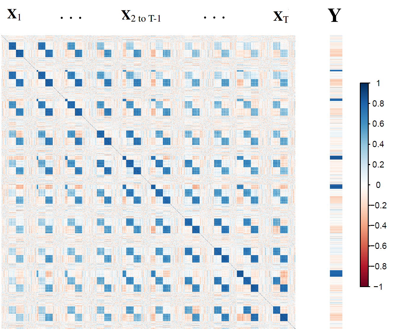
Figure 3: Example of a empirical correlation matrix calculated on a data set simulated with $n=100$, $T=10$, $\rho_{t}=0.9$, $\rho_{d}=0.9$ and $30\%$ of missing values. Correlation scale: from red (-1) to blue (+1)

In the simulation study of Section 4.3, various values for the parameters $n$, $\rho_{t}$, $\rho_{d}$ and the proportion of missing values were considered.

4.2 Competing Methods

mdd-sPLS (with Koh-Lanta algorithm) was compared to several competing methods. Since existing approaches are mostly “two-steps methods”, it is therefore necessary to choose imputation method and prediction method.

The imputation methods selected for this simulation study were:

• mean: this is the simplest way to impute. For a given covariate in a given block, the missing values are estimated with the mean of the non missing values of this covariate.

• softImpute, see Hastie et al. (2015): the imputation is based on the use of fast-ALS dedicated to estimate missing values in a single-block context. Hence, the block structure of the data set is ignored.

• imputeMFA, from the package missMDA, see Husson and Josse (2013): the underlying algorithm takes into account the block structure.

• nipals, suggested by mixOmics authors among other sources: this imputation step is followed by a classic-sPLS. The protocol suggested by the authors is detailed on http://mixomics.org/methods/missing-values/.

Note that the last three imputation methods look for a SVD-modified component-wise structure of the data, as in the proposed mdd-sPLS (with Koh-Lanta algorithm). However, those imputation baseline methods are not supervised and so the number of axes must be tuned by the user.

For the prediction step, three methods were selected:

• mdd-sPLS: the proposed method applied to the imputed data set (i.e. without missing values).

• $\mathcal{L}$asso: the well-known $\mathcal{L}_{1}$-penalized prediction method which is easily usable if the response variable is univariate.

• classic-sPLS: as previously mentioned, this approach is used once the nipals algorithm has been used to impute missing values.

From these different methods of imputation and prediction, we will compare the numerical behavior of the following 8 methodologies:

1. mdd-sPLS with Koh-Lanta algorithm,

2. nipals + classic-sPLS,

3. imputeMFA + mdd-sPLS,

4. imputeMFA + $\mathcal{L}$asso,

5. softImpute + mdd-sPLS,

6. softImpute + $\mathcal{L}$asso,

7. mean + mdd-sPLS,

8. mean + $\mathcal{L}$asso.

In order to properly evaluate the performance of the different methodologies, a learning (train) sample and a test sample should be considered. The given data set is then splitted into a train data set, ($\mathbf{X^{(train)}}$,$\mathbf{Y^{(train)}}$), and a test data set, ($\mathbf{X^{(test)}}$,$\mathbf{Y^{(test)}}$). Let us discuss the strategy of imputation of the train data set and the test data set for the considered methodologies.

• The Koh-Lanta algorithm allows to deal with missing values in the train and test data sets.

• mean: the missing values have been estimated as the mean of the $\mathbf{X^{(train)}}$ variables. They are used to impute $\mathbf{X^{(train)}}$ and $\mathbf{X^{(test)}}$ data sets.

• imputeMFA: the underlying method is used to impute $\mathbf{X^{(train)}}$, but cannot be applied to $\mathbf{X^{(test)}}$ imputation. Thus the missing values of $\mathbf{X^{(test)}}$ was imputed to the means, estimated from $\mathbf{X^{(train)}}$.

• softImpute: even if the authors consider a mono-block problem, it is possible to build a prediction model of imputation (using the softImpute function), which is used to estimate $\mathbf{X^{(test)}}$ from the imputed $\mathbf{X^{(train)}}$ (using the complete function). Note that, apart from the proposed “all-in-one” method (mdd-sPLS with Koh-Lant algorithm), softImpute is the only method reusing the eigen-spaces constructed on $\mathbf{X^{(train)}}$ to impute $\mathbf{X^{(train)}}$ and $\mathbf{X^{(test)}}$.

• nipals: $\mathbf{X^{(train)}}$ is imputed with the nipals function from mixOmics package. The number of components has been arbitrarily fixed to ncomp=3. As for missMDA, there is no particular reason to reuse the eigen-spaces built to impute the $\mathbf{X^{(train)}}$’s missing values to predict the $\mathbf{X^{(test)}}$’s missing values. Thus the $\mathbf{X^{(test)}}$’s missing values are imputed to the mean of the $\mathbf{X^{(train)}}$ data set. Note that the estimation of the classic-sPLS model is based on the imputed $\mathbf{X^{(train)}}$ and $\mathbf{Y^{(train)}}$.

4.3 Simulation Results

The simulation study splits into five parts in order to evaluate:

• the effect of the proportion of missing values,

• the effect of the number of individuals,

• the effect of the inter-block correlation structure,

• the effect of the intra-block correlation structure,

• the computation time and the convergence (of the underlying algorithm) efficiency.

The error considered is the leave-one-out cross-validation root mean square error, denoted RMSEP. For the mdd-sPLS, eight different values were tested for $\lambda$ and the one with the lowest RMSEP error is selected. For the $\mathcal{L}$asso, the glmnet package is used to select the lambda.1se regularization coefficient as proposed by the authors when the low sample size is small. For nipals, softImpute and imputeMFA, the number of components is fixed to $3$. Moreover, eight different values were tested for the softImpute parameter and the most accurate was selected.

The various scenarios considered are inspired by real case problems. For each of the simulation settings, $20$ data sets were generated from the data generating process describes in Section 4.1. Then the eight methodologies presented in section 4.2 were applied to each of the data sets and the associated RMSEP were calculated.

4.3.1 Effect of the Proportion of Missing Values

For the eight methodologies considered, Table 1 provides the RMSEP errors for eight different proportions of missing values from $2\%$, to $60\%$ when the data generating process is based on $\rho_{d}=0.9$, $\rho_{t}=0.9$ (i.e. strong inter/intra-blocks correlations) with $n=100$. Figure 4 shows the performances of the methods.

			2%	5%	8%	10%	15%
	Imputation	Prediction
RMSEP	mdd-sPLS (with Koh-Lanta)		0.243 $\pm$ 0.0535	0.259 $\pm$ 0.0560	0.255 $\pm$ 0.0588	0.260 $\pm$ 0.0582	0.282 $\pm$ 0.0610
	nipals	classic-sPLS	0.251 $\pm$ 0.0514	0.282 $\pm$ 0.0545	0.296 $\pm$ 0.0523	0.313 $\pm$ 0.0510	0.366 $\pm$ 0.0540
	imputeMFA	mdd-sPLS	0.253 $\pm$ 0.0542	0.283 $\pm$ 0.0555	0.291 $\pm$ 0.0567	0.307 $\pm$ 0.0549	0.347 $\pm$ 0.0553
	imputeMFA	Lasso	0.218 $\pm$ 0.0460	0.259 $\pm$ 0.0495	0.269 $\pm$ 0.0425	0.292 $\pm$ 0.0442	0.335 $\pm$ 0.0484
	softImpute	mdd-sPLS	0.251 $\pm$ 0.0531	0.281 $\pm$ 0.0547	0.290 $\pm$ 0.0550	0.304 $\pm$ 0.0531	0.347 $\pm$ 0.0554
	softImpute	Lasso	0.215 $\pm$ 0.0445	0.255 $\pm$ 0.0471	0.267 $\pm$ 0.0403	0.289 $\pm$ 0.0431	0.332 $\pm$ 0.0465
	Mean	mdd-sPLS	0.253 $\pm$ 0.0541	0.284 $\pm$ 0.0553	0.292 $\pm$ 0.0566	0.308 $\pm$ 0.0551	0.348 $\pm$ 0.0557
	Mean	Lasso	0.219 $\pm$ 0.0455	0.260 $\pm$ 0.0495	0.271 $\pm$ 0.0430	0.293 $\pm$ 0.0437	0.337 $\pm$ 0.0477
			20%	30%	40%	50%	60%
	Imputation	Prediction
RMSEP	mdd-sPLS (with Koh-Lanta)		0.300 $\pm$ 0.0625	0.315 $\pm$ 0.0488	0.362 $\pm$ 0.0598	0.413 $\pm$ 0.0555	0.519 $\pm$ 0.0639
	nipals	classic-sPLS	0.407 $\pm$ 0.0475	0.475 $\pm$ 0.0439	0.561 $\pm$ 0.0474	0.639 $\pm$ 0.0412	0.747 $\pm$ 0.0418
	imputeMFA	mdd-sPLS	0.380 $\pm$ 0.0516	0.426 $\pm$ 0.0480	0.488 $\pm$ 0.0536	0.544 $\pm$ 0.0473	0.634 $\pm$ 0.0480
	imputeMFA	Lasso	0.379 $\pm$ 0.0525	0.437 $\pm$ 0.0578	0.516 $\pm$ 0.0615	0.584 $\pm$ 0.0618	0.688 $\pm$ 0.0688
	softImpute	mdd-sPLS	0.379 $\pm$ 0.0519	0.425 $\pm$ 0.0475	0.487 $\pm$ 0.0539	0.541 $\pm$ 0.0469	0.624 $\pm$ 0.0471
	softImpute	Lasso	0.378 $\pm$ 0.0518	0.437 $\pm$ 0.0556	0.514 $\pm$ 0.0588	0.582 $\pm$ 0.0576	0.676 $\pm$ 0.0638
	Mean	mdd-sPLS	0.381 $\pm$ 0.0523	0.426 $\pm$ 0.0479	0.489 $\pm$ 0.0539	0.544 $\pm$ 0.0465	0.628 $\pm$ 0.0473
	Mean	Lasso	0.382 $\pm$ 0.0524	0.441 $\pm$ 0.0548	0.517 $\pm$ 0.0596	0.584 $\pm$ 0.0579	0.679 $\pm$ 0.0643

Table 1: Effect of proportion of missing values on the RMSEP. $100$ simulation results for ($\rho_{d}=0.9,\rho_{t}=0.9$) and $n=100$ individuals. The main statistics are given for each method with (mean $\pm$ std). Bolded results correspond to best results for a given proportion of missing values.

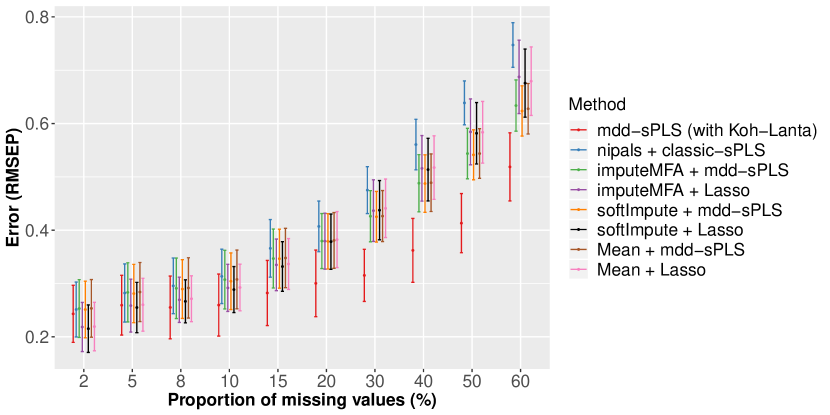
Figure 4: Effect of proportion of missing values on the RMSEP, barplot of Table 1 results.

For small proportions of missing values, all the methodologies provide very similar results with a very slight advantage to the $\mathcal{L}$asso based regression methods. When the proportion of missing values increases, two methods behaved differently compared to the others (Figure 4). From 20% of missing values onward, The mdd-sPLS with Koh-Lanta gave clearly better results than the others methods. When the proportion of missing values is at 50% or more, nipals + classic-sPLS methods provides poorer results compared to all the other approaches.

4.3.2 Effect of the Number n of Individuals

For the eight methodologies considered, Table 2 provides the RMSEP errors for different numbers $n$ of individuals ($n=100,50,20$) when the data generating process is based on $\rho_{d}=0.9$, $\rho_{t}=0.9$ (i.e. strong inter/intra-blocks correlations) with a proportion of missing values equal to 30%. Table 2 provides RMSEP error results for these different numbers $n$ of individuals.

			100	50	20
	Imputation	Prediction
RMSEP	mdd-sPLS (with Koh-Lanta)		0.308 $\pm$ 0.0528	0.335 $\pm$ 0.0643	0.445 $\pm$ 0.139
	nipals	classic-sPLS	0.491 $\pm$ 0.0504	0.497 $\pm$ 0.0665	0.566 $\pm$ 0.124
	imputeMFA	mdd-sPLS	0.420 $\pm$ 0.0530	0.440 $\pm$ 0.0648	0.521 $\pm$ 0.119
	imputeMFA	Lasso	0.438 $\pm$ 0.0599	0.506 $\pm$ 0.0852	0.714 $\pm$ 0.169
	softImpute	mdd-sPLS	0.420 $\pm$ 0.0525	0.436 $\pm$ 0.0644	0.505 $\pm$ 0.119
	softImpute	Lasso	0.436 $\pm$ 0.0581	0.496 $\pm$ 0.0824	0.656 $\pm$ 0.162
	Mean	mdd-sPLS	0.421 $\pm$ 0.0527	0.440 $\pm$ 0.0666	0.528 $\pm$ 0.125
	Mean	Lasso	0.440 $\pm$ 0.0593	0.504 $\pm$ 0.0866	0.721 $\pm$ 0.188

Table 2: Effect of sample size on the RMSEP. $100$ simulation results for ($\rho_{d}=0.9,\rho_{t}=0.9$) and $30\%$ of missing values. The main statistics are given for each method with (mean $\pm$ std). Bolded results correspond to best results for a given number of individuals per sample.

The mdd-sPLS with Koh-Lanta leads to the smallest RMSEP error for the three different sample size $n$. The other mdd-sPLS-based methods have better behavior than the $\mathcal{L}$asso-based methods regardless of the imputation method chosen. Finally, the “two-steps method” softImpute + mdd-sPLS has the second best performance.

4.3.3 Effect of the Inter-Block Correlations

As presented before, the response variable in $\bf Y$ was correlated to some covariates of some $X_{t}$’s blocks with the intensity $\rho_{t}$. Moreover the correlation between different $\bf X_{t}$’s blocks was also equal to $\rho_{t}$. The performances of the methods were evaluated according to the parameter $\rho_{t}$ with $\rho_{t}\in\{0.9,0.7,0.5,0.3\}$. Simulation results are provided in Table 3 and are plotted in Figure 9.

			0.9	0.7	0.5	0.3
	Imputation	Prediction
RMSEP	mdd-sPLS with Koh-Lanta		0.312 $\pm$ 0.0516	0.528 $\pm$ 0.0801	0.662 $\pm$ 0.0948	0.752 $\pm$ 0.0896
	nipals	classic-sPLS	0.470 $\pm$ 0.0451	0.602 $\pm$ 0.0662	0.699 $\pm$ 0.0779	0.766 $\pm$ 0.0751
	imputeMFA	mdd-sPLS	0.421 $\pm$ 0.0487	0.572 $\pm$ 0.0710	0.678 $\pm$ 0.0848	0.756 $\pm$ 0.0822
	imputeMFA	Lasso	0.438 $\pm$ 0.0537	0.598 $\pm$ 0.0740	0.724 $\pm$ 0.103	0.816 $\pm$ 0.0975
	softImpute	mdd-sPLS	0.420 $\pm$ 0.0492	0.570 $\pm$ 0.0706	0.677 $\pm$ 0.0853	0.754 $\pm$ 0.0824
	softImpute	Lasso	0.433 $\pm$ 0.0533	0.591 $\pm$ 0.0723	0.718 $\pm$ 0.102	0.813 $\pm$ 0.100
	Mean	mdd-sPLS	0.421 $\pm$ 0.0492	0.572 $\pm$ 0.0713	0.679 $\pm$ 0.0858	0.756 $\pm$ 0.0827
	Mean	Lasso	0.436 $\pm$ 0.0538	0.598 $\pm$ 0.0743	0.724 $\pm$ 0.105	0.818 $\pm$ 0.0996

Table 3: Effect of inter-block correlation on the RMSEP. $100$ simulation results for $\rho_{d}=0.9$, $\rho_{t}\in\{0.3,0.5,0.7,0.9\}$, $n=100$ individuals and $30\%$ of missing values. The main statistics are given for each methodology with (mean $\pm$ std). Bolded results correspond to the best ones for a given value of $\rho_{t}$.

For any $\rho_{t}$, the mdd-sPLS with Koh-Lanta method is the most accurate one according to the RMSEP. For low values of $\rho_{t}$, the mdd-sPLS-based methods showed better behaviors than the $\mathcal{L}$asso-based ones.

4.3.4 Effect of the Intra-Block Correlations

The following simulations evaluate the impact of a varying intra-correlation on the overall error RMSEP. The other parameters have been fixed to $\rho_{t}=0.9$ and $30\%$ of missing values. Simulations results are provided in Table 4 and are plotted in Figure 10.

			0.3	0.5	0.7	0.9
	Imputation	Prediction
RMSEP	mdd-sPLS with Koh-Lanta		0.399 $\pm$ 0.054	0.346 $\pm$ 0.0563	0.317 $\pm$ 0.0482	0.312 $\pm$ 0.0516
	nipals	classic-sPLS	0.538 $\pm$ 0.0524	0.499 $\pm$ 0.0492	0.485 $\pm$ 0.0453	0.47 $\pm$ 0.0451
	imputeMFA	mdd-sPLS	0.477 $\pm$ 0.0534	0.443 $\pm$ 0.0533	0.433 $\pm$ 0.0468	0.421 $\pm$ 0.0487
	imputeMFA	Lasso	0.565 $\pm$ 0.0691	0.504 $\pm$ 0.0608	0.472 $\pm$ 0.0554	0.438 $\pm$ 0.0537
	softImpute	mdd-sPLS	0.476 $\pm$ 0.0524	0.443 $\pm$ 0.0541	0.433 $\pm$ 0.0467	0.42 $\pm$ 0.0492
	softImpute	Lasso	0.565 $\pm$ 0.0661	0.503 $\pm$ 0.0591	0.472 $\pm$ 0.0531	0.433 $\pm$ 0.0533
	Mean	mdd-sPLS	0.476 $\pm$ 0.0527	0.443 $\pm$ 0.0541	0.434 $\pm$ 0.0469	0.421 $\pm$ 0.0492
	Mean	Lasso	0.572 $\pm$ 0.0697	0.508 $\pm$ 0.0604	0.476 $\pm$ 0.0533	0.436 $\pm$ 0.0538

Table 4: Effect of intra-block correlation on the RMSEP. 100 simulation results for $\rho_{t}=0.9$, $\rho_{d}\in\{0.3,0.5,0.7,0.9\}$, $n=100$ individuals and $30\%$ of missing values. The main statistics are given for each methodology with (mean $\pm$ std). Bolded results correspond to the best ones for a given value of $\rho_{d}$.

Among the four simulated settings, the case $\rho_{d}=0.9$ corresponds to an already discussed one, see Figure 4. It is interesting to see the stability of the results for those new simulations. The data set with $\rho_{d}=0.7$ shows that all the method are equivalent ($\approx 0.31$) except mdd-sPLS (with Koh-Lanta) for which the error is lower ($\approx 0.27$). For higher intra-block correlations, among the baseline imputation methods, the Lasso based prediction methods are more efficient than mdd-sPLS ones but mdd-sPLS (with Koh-Lanta) show lowest errors. For lower intra-block correlations, $\rho\in\{0.3,0.5\}$, among the baseline imputation methods, the Lasso based prediction methods are less efficient than mdd-sPLS but mdd-sPLS (with Koh-Lanta) still lead to better results. It is also interesting to notice that the nipals approach has equivalent results than mdd-sPLS prediction based methods with the baseline imputation methods in all features.

4.3.5 Computation Time and Convergence Quality

Regarding the convergence of the various methods, the mean imputation method is not concerned by this numerical aspect since it is based on only one step of imputation. For the other methodologies, once imputation stages have no further effects on subspace estimation, we considered that the imputation process has converged. The convergence criterion was defined as the stabilization of estimations in the last estimated subspace with a threshold value set to $10^{-9}$ and the maximum number of iterations to $100$. More precisely, let us specify for each method the concerned matrix:

• mdd-sPLS: the matrix $\mathbf{T}_{super}\mathbf{V}_{ort}$, which is defined in the algorithm of the method.

• softImpute: the matrix $U$ of the left-singular vectors (Hastie et al., 2015, Algorithm 2.1),

• imputeMFA: the matrix $\mathbf{U}$ of the left-singular vectors (Josse and Husson, 2016, Chapter 3.1),

• nipals: the matrix of the components $\mathbf{t_{k}}$ (Wold et al., 1983, Algorithm 3c). Since the $\mathbf{t}_{k}$’s are obtained by deflation, the test of convergence is done on each component separately. If one of the components does not converge, we consider that the algorithm did not converge and if all the components converge, then the number of iterations is the mean of the total number of iterations.

$100$ simulated data sets have been generated with $T=10$ blocks of $p=160$ covariates (with $\rho_{d}=0.9$ and $\rho_{t}=0.9$), $30\%$ of missing values and $n\in\{100,50,20\}$. For each considered method, results on convergence rate and number of iterations are presented in the first two parts of Table 5. The prediction errors have also been computed and are represented in Figure 11.

			100	50	20
	Imputation	Prediction
Conv. rate	mdd-sPLS with Koh-Lanta		100 %	100 %	100 %
	nipals		100 %	100 %	100 %
	imputeMFA		99.4 %	98.8 %	99.8 %
	softImpute		71.5 %	85.9 %	92.3 %
$\#$ iterations	mdd-sPLS with Koh-Lanta		3 $\pm$ 0	3 $\pm$ 0	3 $\pm$ 0
	nipals		42.6 $\pm$ 8.64	39.2 $\pm$ 8.29	48.7 $\pm$ 7.71
	imputeMFA		27.0 $\pm$ 10.1	29.7 $\pm$ 11.5	31.2 $\pm$ 8.91
	softImpute		71 $\pm$ 13.3	66.6 $\pm$ 12.9	72.7 $\pm$ 12.5
Time (s)	mdd-sPLS with Koh-Lanta		0.662 $\pm$ 0.209	0.343 $\pm$ 0.0403	0.315 $\pm$ 0.0550
	nipals	classic-sPLS	33.0 $\pm$ 5.27	18. $\pm$ 3.77	22.1 $\pm$ 3.48
	imputeMFA	mdd-sPLS	9.44 $\pm$ 3.39	3.93 $\pm$ 1.45	3.12 $\pm$ 0.600
	softImpute	mdd-sPLS	2.00 $\pm$ 0.984	0.849 $\pm$ 0.155	1.14 $\pm$ 0.175
	Mean	mdd-sPLS	0.0124 $\pm$ 0.00215	0.00683 $\pm$ 0.00069	0.00410 $\pm$ 0.000469

Table 5: Effect of number of individuals. $100$ simulation results for $T=10$ blocks of $p=160$ covariates (with $\rho_{d}=0.9$ and $\rho_{t}=0.9$) and for $30\%$ of missing values. The main statistics (over the $100$ simulations) are given for each method with (mean $\pm$ std). That table is divided in three parts. The first part (lines 1 to 4) corresponds to the convergence rate for each imputation method. The second part (lines 5 to 8) corresponds to the number of iterations for each imputation method, only in case of convergence. The Mean imputation method (that works in 1 iteration and thus always converges) is not taken into account in those two parts. The third part (lines 9 to 13) corresponds to the computation time for each method. $mean$’s are calculated not only over the $100$ simulated data sets but also over the number of individuals (indicated in the column and having an impact on leave-one-out computations) in order to “standardize” the results to the time to that of creating a single model one model. Bolded results correspond to best results for a given number $n$ of individuals.

nipals and mdd-sPLS with Koh-Lanta get $100\%$ convergence. imputeMFA almost always converged while for softImpute almost $30\%$ of imputation processes did not converge when $n=100$. Concerning the number of iterations, denoted $\#$ iterations in Table 5, the mdd-sPLS with Koh-Lanta only needs $3$ iterations before converging. softImpute shows a high number of iterations. nipals needed less iterations to converge. imputeMFA used an average of $\sim 30$ iterations with a large standard deviation relatively to the other methods.

Computations have been performed on Intel® Xeon® CPU E5-2690 v2, 3.00GHz processors. Concerning the computation time, one notice that the Mean process naturally is the fastest. This intuitive result is followed by the mdd-sPLS with Koh-Lanta approach for which the computation time lasts $\sim 0.5$ seconds. On the contrary the nipals method lasts within tens of seconds, imputeMFA is faster but still lasts within seconds (from 3.1 to 9.4 seconds). The softImpute method is faster, less than $2$ seconds. Not surprisingly, the computation time of almost all methods decreased as the number $n$ of individuals decreased, with the exception of the nipals and softImpute algorithms.

4.3.6 Conclusion from the Simulations

In comparison with the other competing methods, mddsPLS with Koh-Lanta clearly exhibits very good performances in terms of predictive capacities in the context of a large proportion of missing values and small number $n$ of individuals. This is shown in the context of strongly correlated blocks as well as in the context of low inter-block information correlation (small $\rho_{t}$). Another set of simulations show the robustness of the results for low $\rho_{d}$ and low $\rho_{t}$ and is presented in Appendix G.

5 Real Data Application: the Ebola rVSV-ZEBOV Data Set

The current work was inspired by this real data application.

5.1 The Data Set

The application is an early phase vaccine trial evaluating the rVSV-ZEBOV Ebola vaccine already studied by Rechtien et al. (2017). As many modern early vaccine trials it includes small number of participants (here, $n=18$) with heterogeneous and high dimensional data sets carrying a lot of information through numerous covariates allowing a deep evaluation of the response to the vaccine.

More specifically, for each participant, the gene expression in whole blood by RNA-seq and the cellular functionality by cytometry have been measured at four different days $\in\{0,1,3,7\}$ after vaccination. Genes of interest were pre-selected by removing those with a variance less than $0.2$ leading to $18~{}301$ genes included in the following analysis. The cellular functionality consisted in the characterization of Natural killers, Dendritic cells and Cytokines, covering a total of 129 variables. So, $T=8$ blocks ${\bf X}_{t}$ of covariates were available, see Table 6 for the number of covariates in each ${\bf X}_{t}$’s blocks.

Moreover, the antibody responses against the Gueckedou strain by ELISA have been measured at days $\in\{28,56,84,180\}$ after vaccination, so ${\bf Y}\in\mathbb{R}^{18\times 4}$. The aim of the analysis was to find the best predictors of the antibody responses among the gene expression (transcriptome) and the cellular functionality.

Recall that the mdd-sPLS method works with standardized variables. This standardization step implies that the information contained in the variance is not taken into account for each of the variables.

Type	RNA-SEQ				Cellular functionality
Block	${\bf X}_{1}$	${\bf X}_{2}$	${\bf X}_{3}$	${\bf X}_{4}$	${\bf X}_{5}$	${\bf X}_{6}$	${\bf X}_{7}$	${\bf X}_{8}$
Day	0	1	3	7	0	1	3	7
$\#(variables)$	10279	10134	9082	9670	129	129	129	129

Table 6: Number of covariates per block ${\bf X}_{t}$.

Because of the sample quality constraints, gene expression was not available in about 30% of cases leading to missing values. For example, Table 7 shows the absence (in blue) of all the RNA-Seq values for a particular individual (in columns) for a particular day (in rows) depicting around $30\%$ of missing values. The data set used in that table is available on the NCBI repository.

Individuals	7	5	9	1	15	10	14	4	2	12	17	16	8	18	13	11	3	6
Day 0: $\mbox{Vec}({\bf X}_{1}^{T})^{T}$
Day 1: $\mbox{Vec}({\bf X}_{2}^{T})^{T}$
Day 3: $\mbox{Vec}({\bf X}_{3}^{T})^{T}$
Day 7: $\mbox{Vec}({\bf X}_{4}^{T})^{T}$

Table 7: Missing values (in blue) in the Ebola rVSV-ZEBOV RNA-Seq data sets ${\bf X}_{t},~{}t=1,\dots,4$, where the notation Vec stands for the Vec operator. For a given individual and a given day, all the corresponding values are missing.

5.2 Statistical Analysis

Four mdd-sPLS-based methodologies were compared through MSEP (means square error of prediction) calculated by leave-one-out cross-validation:

• mdd-sPLS with Koh-Lanta,

• two-step approach: imputation to the mean + mdd-sPLS,

• two-step approach: imputation with softImpute + mdd-sPLS,

• two-step approach: imputation with imputeMFA + mdd-sPLS.

Figure 5 focuses on mdd-sPLS with Koh-Lanta and mean + mdd-sPLS and shows the number of times each response variable has been selected for every optimal $\lambda$ value. All comparisons are provided in Table 9. Since the softImpute method uses random initialization and does not converge systematically, a variability appears in the prediction errors, here depicted by the ($mean\pm std$) notation. All the methods led to the selection of the day 56 response variable in the model, the only variable that was always selected by the four methods. mdd-sPLS with Koh-Lanta clearly retains two response variables in the model: day 56 and day 84.

		Leave-One-Out prediction error
Method		Day 28		Day 56		Day 84		Day 180		Mean
Imputation	Prediction	RMSEP	$\#$	RMSEP	$\#$	RMSEP	$\#$	RMSEP	$\#$	RMSEP
mdd-sPLS with Koh-lanta		1.027	4/18		18/18			1.029	1/18	0.9035
$\lambda=0.8654$				0.6143		0.9426	17/18
Mean	mdd-sPLS	1.028	2/18		18/18			1.029	0/18	0.9326
	$\lambda=0.863$			0.6312		1.041	6/18
softImpute	mdd-sPLS	1.029$\pm$0	($0\pm 0$)/18		($18\pm 0$)/18			1.029$\bf\pm 0.0001374$	($0.3\pm 0.5$)/18	0.9294
	$\lambda=0.8566667$			$0.6326\pm 0.03795$		$1.027\pm 0.002191$	($4.4\pm 0.8$)/18
imputeMFA	mdd-sPLS	1.028	3/18		18/18			1.029	0/18	0.9433
	$\lambda=0.852222$			0.6899		1.026	7/18

Table 8: Results of the leave-one-out cross-validation prediction errors applied to the rVSV data set. The last column gives the mean error. The # symbol represents the number of times each variable is selected in the cross-validation process, among $18$ different models built in the cross-validation process (since $n=18$).

Table 9 shows the final model, selected as minimum for day 56, with $\lambda\simeq 0.866$. The mdd-sPLS with Koh-Lanta approach was highly selective as it kept three covariates while the other methods kept $15$ variables  (see Rechtien et al., 2017, Figure S5 from supplementary materials). As mentionned before, the selection over the $\bf Y$ part was also efficient and kept 2 response variables in the model: the antibody levels at day 56 and day 84.

Finally, the selected covariates were biologically meaningful. The three genes (TIFA_{day 1}, SLC6A9_{day 3}, FAM129B_{day 3}) selected through the proposed approach were also selected by Rechtien et al. (2017) as the three top genes in the sensibility analysis realized with bootstrap analysis. Note that the other three methodologies selected the same three covariates except for the softImpute+mdd-sPLS methods which did not select SLC6A9_{day 3}, the corresponding results are not provided here. For each selected covariate in Table 9, the absolute value of the product between the corresponding weight and super-weight gives a measure of its impact in the model. For TIFA_{day 1}, this value was equal to $0.961$, for SLC6A9_{day 3} equal to $0.107$ and for FAM129B_{day 3} equal to $0.255$. The interpretation was that TIFA_{day 1} was the most important covariate while FAM129B_{day 3} was the second most important one and SLC6A9_{day 3} was the third most important one. Correlations, considering only present samples, between TIFA_{day 1} and Gueckedou strain on days $\in\{28,56,84,180\}$ are respectively equal to $0.83$, $0.96$, $0.90$ and $0.81$.

It is also interesting to interpret the parsimony of the antibody response measurements by selecting day 56 and day 84 and not response measurements at day 28 and day 180. This reflects probably the fact that once established, the antibody response is quite stable over every individual and therefore does not need many repeated measurements to be characterized.

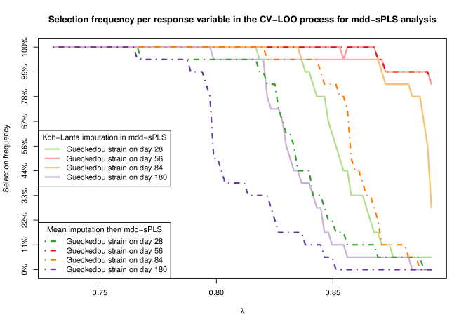
Figure 5: Proportion of selection of each $\mathbf{Y}$ variable for both considered methods on the rVSV data set through Leave-One-Out Cross-Validation. Dotted lines show mean-imputation results and bolded lines full mdd-sPLS with the Koh-Lanta algorithm.

	Block	Variable	Weights	Super-weights
X	Genes on day 1	TIFA	1	-0.961
	Genes on day 3	SLC6A9	0.388	0.277
		FAM129B	0.922
Y	Response	Gueckedou on day 56	-0.924	$\times$
		Gueckedou on day 84	-0.382

Table 9: Ebola rVSV phase I/II constructed mdd-sPLS model for $\lambda=0.8654$. $4$ blocks of gene expression and $4$ blocks of cellular functionality, one for each of the days $\{0,1,3,7\}$, have been introduced but only days $1$ and $3$ blocks of gene expression have been selected. Also, in the response block, only days $56$ and $84$ have been selected. In columns are represented the weights which denote $u_{t}^{(1)}$ for the $\mathbf{X}$ blocks and $v^{(1)}$ for the $\mathbf{Y}$ block and also the super-weights for the $\mathbf{X}$ blocks and denoted by $\beta_{t}^{(1)}$. Only one dimension was found interesting here.

6 Conclusion

The mdd-sPLS method is a SVD-based method (without iteration process) dedicated to multi-block supervised analysis. The Koh-Lanta algorithm deals with missing values in the train sample but also in the test sample and is implemented in the mdd-sPLS method. The considered method shows very good performance on simulated data sets and gave relevant results in the real data application. This approach allows to make variable selection and missing values imputation. The missing data context is limited to entire rows of missing values for certain blocks and can be generalized to any position of missing values by adjusting missing values thanks to known values through a linear model for example. Most of the results, described in this paper, relate to regression problem but the method can also be applied to classification problem.

The mdd-sPLS including Koh-Lanta algorithm method has been implemented in:

• a R-package accessible on the CRAN, https://cran.r-project.org/package=ddsPLS,

• a python-package accessible on PyPi, https://pypi.org/project/py_ddspls/.

Appendix A Monotonicity of the Weight Cardinality: a Counter Example

The remaining question is about the potential decreasing of the number of variables selected per component. In other words, is the number of null coefficients of a given component a decreasing function of $\lambda$? The answer is no as we will see through the following counterexample.

A sample of $n=100$ individuals is generated with the following correlation structure between a 9-dimensional covariate and a two-dimensional response:

$\frac{\mathbf{Y}^{T}\mathbf{X}}{n-1}=$ $X_{1}$ $X_{2}$ $X_{3}$ $X_{4}$ $X_{5}$ $X_{6}$ $X_{7}$ $X_{8}$ $X_{9}$ $Y_{1}$ 1.00 -0.06 -0.10 0.07 0.09 0.15 0.16 0.14 0.22 $Y_{2}$ -0.08 0.98 0.29 -0.18 0.25 0.02 0.04 -0.01 -0.03 .

The $1^{st}$ and the $2^{nd}$ $\mathbf{X}$-variables are clearly well correlated respectively with the $1^{st}$ and the $2^{nd}$ $\mathbf{Y}$-variables. Let us denote by $\bf u$, respectively $\bf v$, the first right, respectively left, eigen vector of the soft-thresholded covariance matrix $S_{\lambda}(\frac{\mathbf{Y}^{T}\mathbf{X}}{n-1})$ for any positive $\lambda$. Figure 6 shows the real cardinalities (black lines) and the upper bound cardinalities (red lines) of $\bf u$ and $\bf v$ weights which correspond the application of Corollary 2.1.1. Vertical lines (discontinuous blue lines) symbolize the vanishing of a coefficient of the current matrix $S_{\lambda}(\frac{\mathbf{Y}^{T}\mathbf{X}}{n-1})$, depending on $\lambda$. When $\lambda\in[0.1,0.14]$, $\mathbf{Card}({\bf u})$ increases, this corresponds to an area in which $\mathbf{Card}({\bf u})$ might take the value $9$, in that part all the columns are different from $0$, except for $\lambda=0.14$, where the variable $X_{8}$ “disappears”.

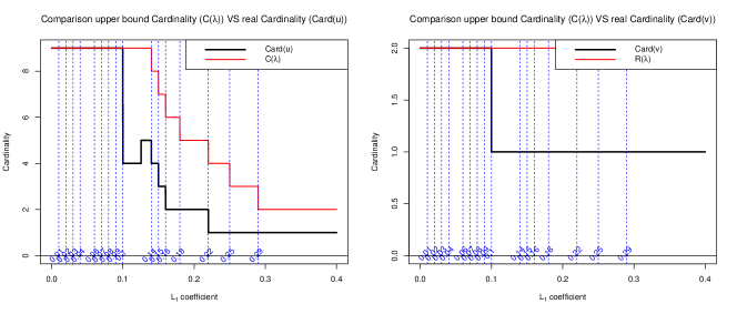
Figure 6: Behaviors of the cardinalities and their upper bounds, defined with corollary 2.1.1, for a simulation case, first component.

Let us zoom on those particular points:

$$\begin{split}u(\lambda=0.12)\approx\begin{matrix}(0,0.97,0.19,-0.07,0.15,0,0,0,0)^{T}\end{matrix}&\rightarrow\mathbf{Card}({\bf u}(\lambda=0.12))=4\\ u(\lambda=0.13)\approx\begin{matrix}(0.99,0,0,0,0,0.023,0.034,0.011,0.10)^{T}\end{matrix}&\rightarrow\mathbf{Card}({\bf u}(\lambda=0.13))=5,\end{split}$$

This is due to the fact that the order of the components associated with the first two-dimensional eigenspace is defined through the $\mathcal{L}_{2}$-norm of the components. However, the $\mathcal{L}_{1}$-shrinkage of the coefficients based on $\lambda$ can change this order since the power of both the first two components are very close to each other, , and only in that case. A way of avoiding this kind of reversal would be to change the soft-thresholding operation with a more $\mathcal{L}_{2}$-shrinkage flavored operation such as the SCAD operation, see for example Fan and Li (2001). But in real cases, the first components are not often sufficiently close in the $\mathcal{L}_{2}$-norm sense to observe this kind of reversal. Thus, it was decided to keep the soft-thresholding operator in the mdds-PLS method.

Appendix B Regression Example: the Liver Toxicity Data Set

In the liver toxicity data set (see Heinloth et al., 2004) $n=64$ male rats of the inbred strain Fisher 334 were exposed to non toxic (50 or 150 mg/kg), moderately toxic (1500 mg/kg) or severely toxic (2000 mg/kg) doses of acetaminophen (paracetamol) in a controlled experiment. The values of $\mathbf{X}\in\mathbb{R}^{64\times 3116}$ are RNA measures and the values of $\mathbf{Y}\in\mathbb{R}^{64\times 10}$ are clinical measures of markers for liver injury. There are no missing values. A comparison of classic-sPLS and the proposed mdd-sPLS is given in Figure 7.

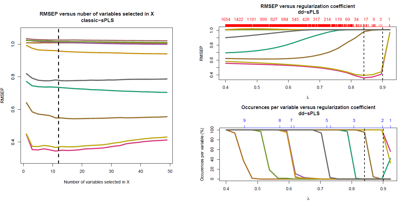
Figure 7: Results of Cross-Validation Leave One Out for both the classic-sPLS and mdd-sPLS methods for the Liver Toxicity data set.

The first two graphics provide the results of leave-one-out cross-validation for the associated tuning parameters: the number of variables for classic-sPLS and the parameter $\lambda$ for mdd-sPLS. The third graphic gives the number of occurrences of each of the ${\bf Y}$’s response variables versus $\lambda$. These 10 response variables are plotted independently, so one curve represents the behavior of one response variable depending on the model and the regularization parameter chosen. Let us comment the results of these two approaches.

• classic-sPLS. According to the suggestion of Lê Cao et al. (2008), the $keep_{Y}$ parameter has arbitrarily been fixed to 2. With this choice, 8 response variables are removed systematically from the built models in the cross-validation process. One hope that the same two response variables are almost always selected, but this is clearly not the case. Indeed, if it were, 8 response variables should have a RMSEP value around 1 (the mean-prediction error, since the variables were standardized), which means that the model does not take into account those variables. However, this observation is only valid for only 5 response. This is problematic because the obtained sparse model strongly depends on this arbitrary choice of the $keep_{Y}$ parameter and thus may provide a wrong model for both selection and prediction.

• mdd-sPLS. The graphic of the RMSEP errors versus $\lambda$ clearly shows that 5 response variables are already estimated to the mean when $\lambda=0.4$ (with corresponding RMSEP errors closed to 1) while the five others are still estimated by the model at this stage. Then, as the regularization parameter $\lambda$ increases, the variability of the RMSEP errors increases since the model has less and less information in the underlying soft-thresholded matrix. By carefully studying this graph, only 2 response variables (the 2 bottom ones) show real learning interest, observable through their decreasing curves while the other curves are increasing. The decreasing part reaches a minimum for $\lambda\approx 0.85$. One can see that this value coincides with the moment when the $3^{rd}$ response variable, in terms of increasing RMSEP ranking, reaches to 1, the symbolic limit of the error. This is equivalent to say that the model doesn’t select that variable.

  The graphic of the occurrences (per response variable) in the estimated models built in the cross-validation process also reinforces the user’s choice to only select two response variables.

Variable		A_43_P14131	A_42_P620915	A_43_P11724	A_42_P802628	A_43_P10606	A_42_P675890	A_43_P23376	A_42_P758454	A_42_P578246	A_43_P17415	A_42_P610788	A_42_P840776	A_42_P705413	A_43_P22616	Mean RMSEP(LOO)	Min RMSEP(LOO)
classic-sPLS	$k_{X}=12$	-0.6	-0.52	0.17	-0.12	-0.14	-0.18	-0.21	-0.18	-0.14	-0.33	-0.07	-0.26			0.78	0.34
mdd-sPLS	$\lambda=0.845$	-0.6	-0.52	0.17	-0.12	-0.14	-0.18	-0.21	-0.18	-0.14	-0.33	-0.07	-0.26	-0.03	-0.01	0.88	0.36
	$\lambda=0.9$	-0.86	-0.51													0.89	0.41

Table 10: Results for classic-sPLS and mdd-sPLS methods: selected genes with their corresponding estimated weights. The two last columns provide the mean and the minimum of the RMSEP errors calculated during the cross-validation process.

Table 10 provides results of $\bf X$’s weights obtained for classic-sPLS and mdd-sPLS with two choices of $\lambda$. Those models have been retained according to Figure 7. classic-sPLS based on mixOmics R package selects 12 genes (with an optimal parameter $keep_{X}$ obtained by cross-validation) and 2 response variables (with the parameter $keep_{y}$ arbitrarily set to 2 by the user). This approach provides the lower cross-validation leave-one-out errors. For the mdd-sPLS method, one can clearly see that the best model, in terms of minimum RMSEP error is not the sparsest one (with 14 genes selected including the 12 genes selected by classic-sPLS). But, looking at the degree of sparsity in $\mathbf{Y}$ also permits to select $\lambda=0.9$ as a good candidate. For that value of $\lambda$ (very close to the optimal one), the number of genes selected goes from 14 to 2 which is a very good model in terms of sparsity. For $\lambda=0.9$, mdd-sPLS (with the first component only) provides an excellent selection simultaneously in $\bf X$ and $\bf Y$, with two variables selected in each matrix and a parameter $\lambda$ close to its optimal value in terms of cross-validation leave-one-out errors.

Appendix C Classification Example: the Penicillium YES Data Set

The Penicillium YES data set (available in the sparseLDA package) is a classification data set describing three Penicillium species: melanoconodium, polonicum, and venetum. In this data set of size $n=36$ (with the three balanced groups), $p=3542$ covariates were extracted from multi-spectral images with 18 spectral bands: $\mathbf{X}\in\mathbb{R}^{36\times 3542}$ and $\mathbf{Y}\in\mathbb{R}^{36\times 3}$ where the three columns of $\bf Y$ are the indicator variables of the groups). More details are available by Clemmensen et al. (2011) where the interest of the Sparse Discriminant Analysis method is highlighted. The Sparse Discriminant Analysis method needed only 2 covariates to perfectly predict the assignment to one of the three groups. A leave-one-out cross-validation has been performed for each fold $i=1,\dots,12$, the $i^{th}$ triplet of melanoconodium, polonicum, and venetum, to optimize the parameter $\lambda$. The mdd-sPLS method (with $\lambda=0.956$ for example) permits to select 4 different covariates, 2 on each of the two components, with a perfect assignment rate. These two components are plotted in Figure 8 and the separation of the three groups is clearly visible.

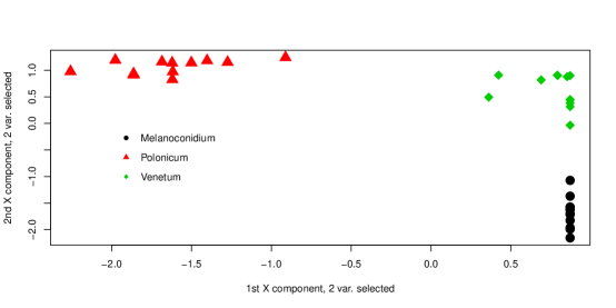
Figure 8: Results of the application of the mdd-sPLS to the Penicillium YES data set.

Appendix D Effect of Varying Inter-Block Correlation

The case of varying inter-block correlation has been analysed in that part. The Figure 9 summarizes the corresponding results. Other parameters have been respectively fixed to $\rho_{d}=0.9$, $30\%$ of missing values, 100 individuals per simulated data set and 100 simulations per $\rho_{t}$.

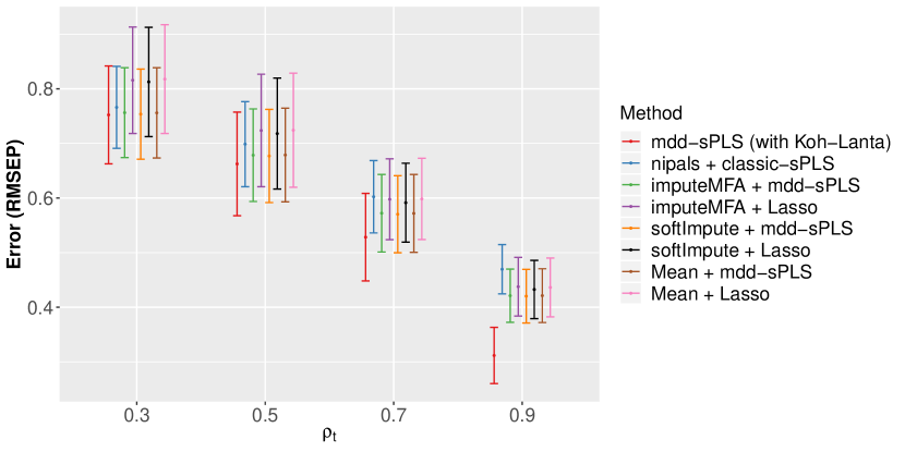
Figure 9: Effect of varying $\rho_{t}$ on the RMSEP, barplot of Table 3 results. For fixed values of $\rho_{d}=0.9$, $30\%$ of missing values, 100 individuals per simulated data set and a total of $100$ simulated data sets

In the context of strongly correlated blocks, mdd-sPLS (with Koh-Lanta) seems to have a better behavior than the other methods where nipals + classic-sPLS is slightly less efficient than other methods where mdd-sPLS prediction based methods are lighlty better than Lasso prediction based methods. As the correlation between blocks shrinks, the mdd-sPLS prediction based methods and mdd-sPLS (with Koh-Lanta) show equivalent results, plus, nipals + classic-sPLS is almost as good as those methods. Finally in that low correlation context, the Lasso prediction based methods, are less efficient than other methods.

Appendix E Effect of Varying Intra-Block Correlation

The case of varying intra-block correlation has been analysed in that part. The Figure 10 summarizes the corresponding results. Other parameters have been respectively fixed to $\rho_{t}=0.9$, $30\%$ of missing values, 100 individuals per simulated data set and 100 simulations per $\rho_{d}$.

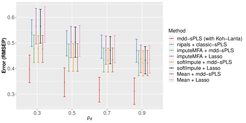
Figure 10: Effect of of varying $\rho_{d}$ on the RMSEP, barplot of Table 4 results. For fixed values of $\rho_{t}=0.9$, $30\%$ of missing values, 100 individuals per simulated data set and a total of $100$ simulated data sets

Whatever is the intensity of the intra-block correlation, mdd-sPLS (with Koh-Lanta) shows better results in terms of prediction error. Furthermore the mdd-sPLS prediction based methods are the second ranked methods. The third position is given to the Lasso prediction based methods for strong intra-block correlations and to nipals + classic-sPLS for low intra-block correlations.

Appendix F Effect of Varying Number of Individuals

The case of varying number of individuals has been analysed in that part. Figure 11 summarizes the corresponding results. Other parameters have been respectively fixed to $\rho_{t}=0.9$, $\rho_{d}=0.9$, $30\%$ of missing values, 100 individuals per simulated data set and 100 simulations per $n$.

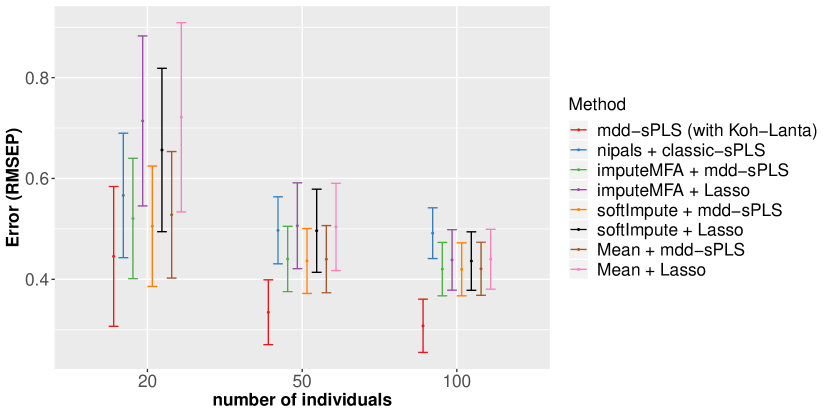
Figure 11: Effect of of varying number of participants on the RMSEP, barplot of Table 5 results. For fixed values of $\rho_{t}=0.9$, $\rho_{d}=0.9$, $30\%$ of missing values and a total of $100$ simulated data sets.

Three cases have been considered. For a low number of individuals, mdd-sPLS (with Koh-Lanta) has the smallest error, the mdd-sPLS prediction based methods and the nipals + classic-sPLS method are slightly less precise and the Lasso prediction based methods are fewer precise. As the number of individuals increase, the nipals + classic-sPLS method seems to be less precise than other methods while mdd-sPLS (with Koh-Lanta) finally gets very better results.

Appendix G Effect of Low Intra-Block and Inter-Block Simulations

The following simulations permit to appreciate the validity of the proposed method if there is little information to catch between blocks (low inter-block correlation) and inside blocks (low intra-block correlation).

Here, the proportion of missing values has been fixed to $30\%$ and the number of individuals to $n=100$. The intra-block correlation has been fixed to $\rho_{d}=0.3$ and the inter-block correlation to $\rho_{t}=0.5$. Figure 12 shows the results for $100$ simulated data sets.

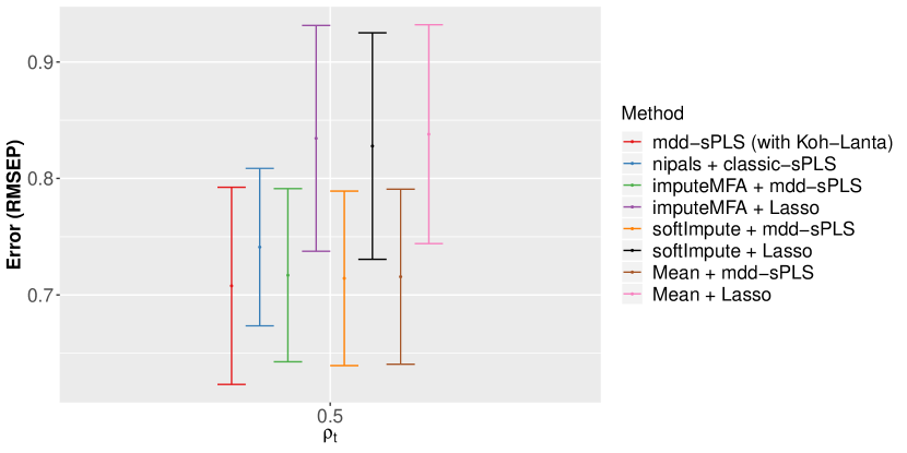
Figure 12: Effect of low intra-block correlation, $\rho_{d}=0.3$, and low inter-block correlation, $\rho_{t}=0.5$, on the overall errors for fixed values of of missing values, $30\%$, for $100$ individuals per simulated data set and a total of $100$ simulated data sets.

For that level of information, the all methods show equivalent performances, with an error close to $\approx 0.73$, except for the Lasso based prediction methods, for which the error is higher $\approx 0.83$.

References

- Amini and Wainwright (2008) Arash A Amini and Martin J Wainwright. High-dimensional analysis of semidefinite relaxations for sparse principal components. In Information Theory, 2008. ISIT 2008. IEEE International Symposium on, pages 2454–2458. IEEE, 2008.
- Bertsimas et al. (2018) Dimitris Bertsimas, Colin Pawlowski, and Ying Daisy Zhuo. From predictive methods to missing data imputation: An optimization approach. Journal of Machine Learning Research, 18(196):1–39, 2018. URL http://jmlr.org/papers/v18/17-073.html.
- Bougeard et al. (2011) Stéphanie Bougeard, El Mostafa Qannari, Coralie Lupo, and Mohamed Hanafi. From multiblock partial least squares to multiblock redundancy analysis. a continuum approach. Informatica, 22(1):11–26, 2011.
- Buuren and Groothuis-Oudshoorn (2010) S van Buuren and Karin Groothuis-Oudshoorn. mice: Multivariate imputation by chained equations in r. Journal of statistical software, pages 1–68, 2010.
- Cai and Liu (2011) Tony Cai and Weidong Liu. Adaptive thresholding for sparse covariance matrix estimation. Journal of the American Statistical Association, 106(494):672–684, 2011.
- Chun and Keleş (2010) Hyonho Chun and Sündüz Keleş. Sparse partial least squares regression for simultaneous dimension reduction and variable selection. Journal of the Royal Statistical Society: Series B (Statistical Methodology), 72(1):3–25, 2010.
- Clemmensen et al. (2011) Line Clemmensen, Trevor Hastie, Daniela Witten, and Bjarne Ersbøll. Sparse discriminant analysis. Technometrics, 53(4):406–413, 2011.
- d’Aspremont et al. (2005) Alexandre d’Aspremont, Laurent E Ghaoui, Michael I Jordan, and Gert R Lanckriet. A direct formulation for sparse pca using semidefinite programming. In Advances in neural information processing systems, pages 41–48, 2005.
- Deshpande and Montanari (2016) Yash Deshpande and Andrea Montanari. Sparse pca via covariance thresholding. Journal of Machine Learning Research, 17(141):1–41, 2016. URL http://jmlr.org/papers/v17/15-160.html.
- Fan and Li (2001) Jianqing Fan and Runze Li. Variable selection via nonconcave penalized likelihood and its oracle properties. Journal of the American statistical Association, 96(456):1348–1360, 2001.
- Hastie et al. (2015) Trevor Hastie, Rahul Mazumder, Jason D Lee, and Reza Zadeh. Matrix completion and low-rank svd via fast alternating least squares. Journal of Machine Learning Research, 16(1):3367–3402, 2015. URL http://jmlr.org/papers/volume16/hastie15a/hastie15a.pdf.
- Heinloth et al. (2004) Alexandra N Heinloth, Richard D Irwin, Gary A Boorman, Paul Nettesheim, Rickie D Fannin, Stella O Sieber, Michael L Snell, Charles J Tucker, Leping Li, Gregory S Travlos, et al. Gene expression profiling of rat livers reveals indicators of potential adverse effects. Toxicological Sciences, 80(1):193–202, 2004.
- Höskuldsson (1988) Agnar Höskuldsson. Pls regression methods. Journal of chemometrics, 2(3):211–228, 1988.
- Hosmer and Lemeshow (1989) DW Hosmer and Stanley Lemeshow. Applied logistic regression. 1989. New York: Johns Wiley & Sons, 1989.
- Husson and Josse (2013) François Husson and Julie Josse. Handling missing values in multiple factor analysis. Food quality and preference, 30(2):77–85, 2013.
- Johnstone and Lu (2004) Iain M Johnstone and Arthur Yu Lu. Sparse principal components analysis. Unpublished manuscript, 7, 2004.
- Johnstone and Lu (2009) Iain M Johnstone and Arthur Yu Lu. On consistency and sparsity for principal components analysis in high dimensions. Journal of the American Statistical Association, 104(486):682–693, 2009.
- Jolliffe et al. (2003) Ian T Jolliffe, Nickolay T Trendafilov, and Mudassir Uddin. A modified principal component technique based on the lasso. Journal of computational and Graphical Statistics, 12(3):531–547, 2003.
- Josse and Husson (2016) Julie Josse and François Husson. missmda: a package for handling missing values in multivariate data analysis. Journal of Statistical Software, 70(1):1–31, 2016.
- Krauthgamer et al. (2015) Robert Krauthgamer, Boaz Nadler, Dan Vilenchik, et al. Do semidefinite relaxations solve sparse pca up to the information limit? The Annals of Statistics, 43(3):1300–1322, 2015.
- Lê Cao et al. (2008) Kim-Anh Lê Cao, Debra Rossouw, Christele Robert-Granié, and Philippe Besse. A sparse pls for variable selection when integrating omics data. Statistical applications in genetics and molecular biology, 7(1), 2008.
- Lê Cao et al. (2009) Kim-Anh Lê Cao, Ignacio González, and Sébastien Déjean. integromics: an r package to unravel relationships between two omics data sets. Bioinformatics, 25(21):2855–2856, 2009.
- Manne (1987) Rolf Manne. Analysis of two partial-least-squares algorithms for multivariate calibration. Chemometrics and Intelligent Laboratory Systems, 2(1-3):187–197, 1987.
- Nelson et al. (1996) Philip RC Nelson, Paul A Taylor, and John F MacGregor. Missing data methods in pca and pls: Score calculations with incomplete observations. Chemometrics and intelligent laboratory systems, 35(1):45–65, 1996.
- Penrose (1956) Roger Penrose. On best approximate solutions of linear matrix equations. In Mathematical Proceedings of the Cambridge Philosophical Society, volume 52, pages 17–19. Cambridge University Press, 1956.
- Qin et al. (2001) S Joe Qin, Sergio Valle, and Michael J Piovoso. On unifying multiblock analysis with application to decentralized process monitoring. Journal of chemometrics, 15(9):715–742, 2001.
- Rechtien et al. (2017) Anne Rechtien, Laura Richert, Hadrien Lorenzo, Gloria Martrus, Boris Hejblum, Christine Dahlke, Rahel Kasonta, Madeleine Zinser, Hans Stubbe, Urte Matschl, Ansgar Lohse, Verena Krähling, Markus Eickmann, Stephan Becker, Selidji Todagbe Agnandji, Sanjeev Krishna, Peter G. Kremsner, Jessica S. Brosnahan, Philip Bejon, Patricia Njuguna, Marylyn M. Addo, Claire-Anne Siegrist, Angela Huttner, Marie-Paule Kieny, Vasee Moorthy, Patricia Fast, Barbara Savarese, Olivier Lapujade, Rodolphe Thiébaut, Marcus Altfeld, and Marylyn Addo. Systems vaccinology identifies an early innate immune signature as a correlate of antibody responses to the ebola vaccine rvsv-zebov. Cell Reports, 20(9):2251–2261, 09 2017. ISSN 2211-1247. doi: 10.1016/j.celrep.2017.08.023. URL http://dx.doi.org/10.1016/j.celrep.2017.08.023.
- Rothman et al. (2009) Adam J Rothman, Elizaveta Levina, and Ji Zhu. Generalized thresholding of large covariance matrices. Journal of the American Statistical Association, 104(485):177–186, 2009.
- Sabatier et al. (2003) Robert Sabatier, Myrtille Vivien, and Pietro Amenta. Two approaches for discriminant partial least squares. In Between data science and applied data analysis, pages 100–108. Springer, 2003.
- Sjöström et al. (1986) Michael Sjöström, Svante Wold, and Bengt Söderström. Pls discriminant plots. In Pattern Recognition in Practice, Volume II, pages 461–470. Elsevier, 1986.
- Stekhoven and Bühlmann (2011) Daniel J Stekhoven and Peter Bühlmann. Missforest—non-parametric missing value imputation for mixed-type data. Bioinformatics, 28(1):112–118, 2011.
- Tenenhaus and Tenenhaus (2011) Arthur Tenenhaus and Michel Tenenhaus. Regularized generalized canonical correlation analysis. Psychometrika, 76(2):257, 2011.
- Tenenhaus et al. (2014) Arthur Tenenhaus, Cathy Philippe, Vincent Guillemot, Kim-Anh Le Cao, Jacques Grill, and Vincent Frouin. Variable selection for generalized canonical correlation analysis. Biostatistics, 15(3):569–583, 2014.
- Tibshirani (1996) Robert Tibshirani. Regression shrinkage and selection via the lasso. Journal of the Royal Statistical Society. Series B (Methodological), pages 267–288, 1996.
- Troyanskaya et al. (2001) Olga Troyanskaya, Michael Cantor, Gavin Sherlock, Pat Brown, Trevor Hastie, Robert Tibshirani, David Botstein, and Russ B Altman. Missing value estimation methods for dna microarrays. Bioinformatics, 17(6):520–525, 2001.
- Wangen and Kowalski (1989) LE Wangen and BR Kowalski. A multiblock partial least squares algorithm for investigating complex chemical systems. Journal of chemometrics, 3(1):3–20, 1989.
- Westerhuis and Smilde (2001) Johan A Westerhuis and Age K Smilde. Deflation in multiblock pls. Journal of chemometrics, 15(5):485–493, 2001.
- Westerhuis et al. (1997) Johan A Westerhuis, Pierre MJ Coenegracht, and Coenraad F Lerk. Multivariate modelling of the tablet manufacturing process with wet granulation for tablet optimization and in-process control. International journal of Pharmaceutics, 156(1):109–117, 1997.
- Wold (1966) Herman Wold. Estimation of principal components and related models by iterative least squares. Multivariate analysis, pages 391–420, 1966.
- Wold (1984) S Wold. Three pls algorithms according to sw. In Proc.: Symposium MULDAST (multivariate analysis in science and technology), pages 26–30, 1984.
- Wold et al. (1983) Svante Wold, Harold Martens, and H Wold. The multivariate calibration problem in chemistry solved by the pls method. In Matrix pencils, pages 286–293. Springer, 1983.
- Zou et al. (2006) Hui Zou, Trevor Hastie, and Robert Tibshirani. Sparse principal component analysis. Journal of computational and graphical statistics, 15(2):265–286, 2006.