Quantum simulation scheme of two-dimensional xy-model Hamiltonian with controllable coupling

Abstract

We study a scheme of quantum simulator for two-dimensional xy-model Hamiltonian. Previously the quantum simulator for a coupled cavity array spin model has been explored, but the coupling strength is fixed by the system parameters. In the present scheme several cavity resonators can be coupled with each other simultaneously via an ancilla qubit. In the two-dimensional Kagome lattice of the resonators the hopping of resonator photonic modes gives rise to the tight-binding Hamiltonian which in turn can be transformed to the quantum xy-model Hamiltonian. We employ the transmon as an ancilla qubit to achieve in situ controllable xy-coupling strength.

1 Introduction

In spite of the remarkable advancements of coherent quantum operation the realization of fully controlled quantum computing is severely challenging in quantum information processing technology. On the other hand, significant attention has been paid to quantum spin models as a promising candidate for quantum simulation of many-body effects Georg ; Cirac ; Buluta . Quantum many-body simulation may provide a variety of possibilities to study the properites of many-body systems, realize a new phase of quantum matter, and eventually lead to the scalable quantum computing, which is hard for classical approaches.

Large-scale quantum simulators consisting of many qubits integrated have been experimentally demonstrated to study the quantum phenomena such as many-body dynamics and quantum phase transition. Quantum simulators have been studied in the so-called coupled cavity array (CCA) model, where a two-level atom in the cavity interacts with its own cavity and the hopping of a photon bewteen cavities gives rise to the cavity-cavity coupling. The CCA model has been applied to study the Jaynes-Cummings Hubbard model (JCHM) HartmanNP ; Xue ; Greentree ; Schmidt ; Koch ; Fan and the Bose-Hubbard model Greentree ; Koch to exhibit the phase transition between Mott insulator and superfluid. However, in the CCA model the cavity-cavity hopping amplitude is set by the system parameters and thus not tunable. In recent studies for one-dimensional quantum simulators using trapped cold atoms Nature51 and trapped ion systems Nature53 the coupling strength was tunable.

Previously the superconducting resonators in two-dimensional lattice have been coupled through an interface capacitance, where the resonator-resonator coupling strength is not controllable as the capacitance is fixed NPreview ; AP . For superconducting resonator cavities in circuit-quantum electrodynamics (QED) systems, qubit is located outside of the cavity MDK ; QIP . Hence a qubit can interact with many resonator cavities surrounding the qubit. By using a qubit as a mediator of coupling between many resonators one can obtain a tunable resonator-resonator coupling which is quite different from the coupling by direct photon hopping in the CCA model.

In this study we consider a lattice model of superconducting resonator cavities coupled by ancilla qubits for simulating the quantum xy-model Hamiltonian. The simulation for quantum xy-model has been studied in one-dimensional Hartmann ; Angelakis and two-dimensional Koch JCHM in the CCA model architecture. In the present model the intervening ancilla qubit which couples cavities has controllable qubit frequency. After discarding the ancilla qubit degrees of freedom by performing a coordinate transformation we show that the photon states in the resonators are described by the tight-binding Hamiltonian which, in turn, can be rewritten as the quantum xy-type interaction Hamiltonian. Consequently, the xy-coupling constant depends on the hopping amplitude of the tight-binding Hamiltonian and thus on the ancilla qubit frequency. We consider two-dimensional Kagome lattice model as well as one-dimensional chain model for the quantum simulation of xy-model Hamiltonian and show that the xy-coupling strength is in situ controllable.

2 Hamiltonian of coupled $n$-resonators

In circuit-QED architectures qubits can be coupled with the transmission resonator at the boundaries of the resonator Blais ; Steffen ; Inomata so that we may couple several resonators to a qubit as depicted in Fig. 1 (a). In principle, any kind of qubits are available, but in this study we employ the transmon as the ancilla qubit coupling the resonators with the advantage of controllability. The Hamiltonian of the system with $n$ resonators and an ancilla qubit in Fig. 1(a) is given by

$$H_{nR}=\frac{1}{2}\omega_{a}\sigma^{z}_{a}+\sum^{n}_{p=1}[\omega_{rp}a^{\dagger}_{p}a_{p}-f_{p}(a^{\dagger}_{p}\sigma^{-}_{a}+\sigma^{+}_{a}a_{p})],$$ (1)

where $a^{\dagger}_{p}$ and $a_{p}$ with the frequency $\omega_{rp}$ are the creation and annihilation operators for microwave photon in $p$-th resonator, respectively, and the Pauli matrix $\sigma^{z}_{a}$ with the frequency $\omega_{a}$ represents the ancilla qubit state, and $f_{p}$ is the coupling amplitude between the photon mode in the $p$-th resonator and the ancilla qubit. This Hamiltonian conserves the excitation number

$${\cal N}_{e}=\sum^{n}_{p=1}N_{rp}+(s_{az}+1/2),$$ (2)

where $s_{az}\in\{-1/2,1/2\}$ are the eigenvalue of the operator $S_{az}=\frac{1}{2}\sigma^{z}_{a}$ for ancilla qubit and $N_{rp}$ is the excitation number of oscillating mode in $p$-th resonator. Here, we consider the subspace that ${\cal N}_{e}=1$ and thus $N_{rp}\in\{0,1\}$, that is, the state of resonator is the superposition of zero and one-photon states which was generated in experiments previously Houck ; Hofheinz08 ; Hofheinz09 .

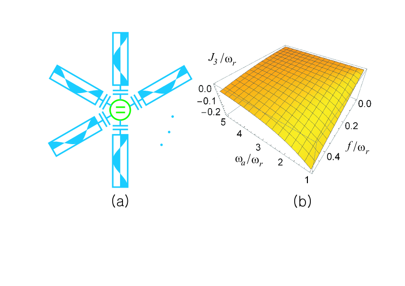
Figure 1: (a) $n$ cavities of circuit-QED resonators are coupled via an intervening ancilla qubit. (b) Effective cavity-cavity coupling, $J_{3}$, for $n=3$ as a function of ancilla qubit frequency $\omega_{a}$ and resonator-ancilla coupling $f$ with the frequency $\omega_{r}$ of resonator photon mode.

In order to obtain the Hamiltonian describing the interaction between photon modes we introduce the transformation

$${\tilde{H}}_{nR}=U^{\dagger}H_{nR}U,$$ (3)

where

$$U=e^{-\sum^{n}_{p=1}\theta_{p}(a^{\dagger}_{p}\sigma^{-}_{a}-\sigma^{+}_{a}a_{p})}.$$ (4)

Here we, for simplicity, assume identical resonators and thus set $\omega_{rp}=\omega_{r},f_{p}=f$ and $\theta_{p}=\theta$. We then expand $U=e^{M}$ with $M=-\sum^{n}_{p=1}\theta_{p}(a^{\dagger}_{p}\sigma^{1}_{a}-\sigma^{+}_{a}a_{p})$ by using the relation $e^{M}=1+M+\frac{1}{2!}M^{2}+\frac{1}{3!}M^{3}+\cdots$ to obtain

$$U_{pp}\!\! = \!\!1-\frac{1}{2!}\theta^{2}\!\!+\!\!\frac{1}{4!}n\theta^{4}\!\!-\!\!\frac{1}{6!}n^{2}\theta^{6}\!\!+\!\!\cdots=\frac{1}{n}(n\!\!-\!\!1\!\!+\!\!\cos\sqrt{n}\theta)$$ (5)

$$U_{n+1,n+1}\!\! = \!\!1-\frac{1}{2!}n\theta^{2}+\frac{1}{4!}n^{2}\theta^{4}-\frac{1}{6!}n^{3}\theta^{6}+\cdots=\cos\sqrt{n}\theta$$ (6)

$$U_{p,n+1}\!\! = \!\!-\theta\!\!+\!\!\frac{1}{3!}n\theta^{3}\!\!-\!\!\frac{1}{5!}n^{2}\theta^{5}\!\!+\!\!\cdots=-\frac{1}{\sqrt{n}}\sin\sqrt{n}\theta=-U_{n+1,p}$$ (7)

$$U_{pq,p\neq q}\!\! = \!\!-\frac{1}{2!}\theta^{2}\!\!+\!\!\frac{1}{4!}n\theta^{4}\!\!-\!\!\frac{1}{6!}n^{2}\theta^{6}\!\!+\!\!\cdots=\frac{1}{n}(\cos\sqrt{n}\theta\!\!-\!\!1).$$ (8)

Here $U$ is a $(n+1)\times(n+1)$ matrix in the basis of $|N_{r1},N_{r2},N_{r3},\cdots,N_{rn},s_{az}\rangle$ and $p,q\in\{1,2,3,\cdots,n\}$.

The degree of freedoms of ancilla qubit and resonator photon modes in the Hamiltonian of Eq. (1) can be decoupled by imposing the condition

$$\tan 2\sqrt{n}\theta=2\sqrt{n}\frac{f}{\Delta}$$ (9)

which can be achieved by adjusting the detuning $\Delta\equiv\omega_{a}-\omega_{r}$ Blais . The resulting transformed Hamiltonian of Eq. (3) becomes

$${\tilde{H}}_{nR}=\left(\begin{array}[]{cccccc}\epsilon^{r}_{1}&J_{n}&J_{n}&\cdots&J_{n}&0\\ J_{n}&\epsilon^{r}_{2}&J_{n}&\cdots&J_{n}&0\\ J_{n}&J_{n}&\epsilon^{r}_{3}&\cdots&J_{n}&0\\ \vdots&\vdots&\vdots&\ddots&\vdots&\vdots\\ J_{n}&J_{n}&J_{n}&\cdots&\epsilon^{r}_{n}&0\\ 0&0&0&\cdots&0&\epsilon^{a}\end{array}\right),$$ (16)

where $\epsilon^{a}$ is the energy for the state that $s_{az}=1/2$ and $N_{rp}=0$ for all $p\in\{1,2,3,\cdots,n\}$, and $\epsilon^{r}_{p}$ is the energy for the state that $s_{az}=-1/2$ and only the $p$-th resonator has one photon, $N_{rp}=1$ and $N_{rq}=0~{}(q\neq p)$. For identical resonators, $\epsilon^{r}_{1}=\epsilon^{r}_{2}=\epsilon^{r}_{3}=\cdots=\epsilon^{r}$ and $\epsilon^{a}$ are explicitly evaluated as

$$\epsilon^{r} = -\frac{1}{2n}\left(\Delta+sgn(\Delta)\sqrt{\Delta^{2}+4nf^{2}}\right)+\frac{1}{2}\omega_{r},$$ (17)

$$\epsilon^{a} = \frac{1}{2}sgn(\Delta)\sqrt{\Delta^{2}+4nf^{2}}+\frac{1}{2}\omega_{r},$$ (18)

and the resonator-resonator coupling is given by

$$J_{n}=\frac{1}{2n}\left(\Delta-sgn(\Delta)\sqrt{\Delta^{2}+4nf^{2}}\right),$$ (19)

where $sgn(\Delta)$ is $+1(-1)$ for $\Delta>0~{}(\Delta<0)$.

In the subspace satisfying ${\cal N}_{e}=1$ the Hamiltonian ${\tilde{H}}_{nR}$ in Eq. (16) can be represented as

$${\tilde{H}}_{nR} = \frac{1}{2}\sum^{2}_{p=1}\omega^{\prime}_{r}(2a^{\dagger}_{p}a_{p}-1)+\sum^{n}_{p,q=1,p\neq q}J_{n}(a^{\dagger}_{p}a_{q}+a_{p}a^{\dagger}_{q})$$ (20)

$$+\frac{1}{2}\omega^{\prime}_{a}\sigma^{z}_{a}.$$

Consequently, $\epsilon^{r}_{p}$ and $\epsilon^{a}$ can be rewritten as $\epsilon^{r}_{p}=\epsilon^{r}=-\frac{n-2}{2}\omega^{\prime}_{r}-\frac{1}{2}\omega^{\prime}_{a}$ and $\epsilon^{a}=-\frac{n}{2}\omega^{\prime}_{r}+\frac{1}{2}\omega^{\prime}_{a}$ so that we can have the relations, $\omega^{\prime}_{a}=-(n\epsilon^{r}-(n-2)\epsilon^{a})/(n-1)$ and $\omega^{\prime}_{r}=-(\epsilon^{r}+\epsilon^{a})/(n-1)$. In this tight-binding Hamiltonian the ancilla qubit operator $\sigma^{z}_{a}$ is decoupled from the resonator photon mode $a$, and afterward we will ignore the ancilla term.

The tight-binding Hamiltonian ${\tilde{H}}_{nR}$ can be easily transformed to the xy-spin model by introducing a pseudo spin operator $\sigma_{p}$ such that $2a_{p}a^{\dagger}_{p}-1=|1_{p}\rangle\langle 1_{p}|-|0_{p}\rangle\langle 0_{p}|=\sigma^{z}_{p}$ and $a^{\dagger}_{p}a_{q}+a_{p}a^{\dagger}_{q}=|1_{p}0_{q}\rangle\langle 0_{p}1_{q}|+|0_{p}1_{q}\rangle\langle 1_{p}0_{q}|=\sigma^{+}_{p}\sigma^{-}_{q}+\sigma^{-}_{p}\sigma^{+}_{q}=(1/2)(\sigma^{x}_{p}\sigma^{x}_{q}+\sigma^{y}_{p}\sigma^{y}_{q})$ as follows:

$$H_{xy}=\frac{1}{2}\sum^{n}_{p=1}\omega^{\prime}_{r}\sigma^{z}_{p}+\frac{1}{2}\sum^{n}_{p,q=1,p\neq q}J_{n}(\sigma^{x}_{p}\sigma^{x}_{q}+\sigma^{y}_{p}\sigma^{y}_{q}).$$ (21)

Here, the hopping parameter $J_{n}$ acts as a xy coupling constant between pseudo spins.

3 xy-model with tunable coupling

Figure 2(a) shows one-dimensional lattice model by extending the structure in Fig. 1(a) for two resonators and an ancilla qubit ($n=2$). The transformation of Hamltonian ${\tilde{H}}_{2R}=U^{\dagger}H_{2R}U$ in Eq. (3) can be evaluated by using the transformation matrix $U=e^{M}=e^{-\sum^{2}_{j=1}\theta_{j}(a^{\dagger}_{j}\sigma^{-}-\sigma^{+}a_{j})}$ with

$$H_{2R}=\left[{\begin{array}[]{ccc}\omega_{r1}-\frac{1}{2}\omega_{a}&0&-f_{1}\\ 0&\omega_{r2}-\frac{1}{2}\omega_{a}&-f_{2}\\ -f_{1}&-f_{2}&\frac{1}{2}\omega_{a}\\ \end{array}}\right],M=\left[{\begin{array}[]{ccc}0&0&-\theta_{1}\\ 0&0&-\theta_{2}\\ \theta_{1}&\theta_{2}&0\\ \end{array}}\right].$$ (28)

For identical resonators such that $\omega_{r1}=\omega_{r2}=\omega_{r},f_{1}=f_{2}=f$, and thus $\theta_{1}=\theta_{2}=\theta$, the transformation matrix can be calculated as

$$U=\left[{\begin{array}[]{ccc}\frac{1}{2}(\cos\sqrt{2}\theta+1)&\frac{1}{2}(\cos\sqrt{2}\theta-1)&-\frac{1}{\sqrt{2}}\sin\sqrt{2}\theta\\ \frac{1}{2}(\cos\sqrt{2}\theta-1)&\frac{1}{2}(\cos\sqrt{2}\theta+1)&-\frac{1}{\sqrt{2}}\sin\sqrt{2}\theta\\ \frac{1}{\sqrt{2}}\sin\sqrt{2}\theta&\frac{1}{\sqrt{2}}\sin\sqrt{2}\theta&\cos\sqrt{2}\theta\\ \end{array}}\right]$$ (32)

with the basis $|N_{r1},N_{r2},s_{az}\rangle\in\{|1,0,-1/2\rangle,|0,1,-1/2\rangle,|0,0,1/2\rangle\}$, the photon number in 1st (2nd) resonator $N_{r1}(N_{r2})$ and the ancilla qubit spin $s_{az}$.

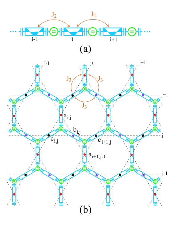
Figure 2: (a) One-dimensional chain of cavity resonators coupled via ancilla qubits with the effective cavity-cavity coupling $J_{2}$. (b) Two-dimensional Kagome lattice of cavity resonators consisting of three triangular sublattices, $a_{i,j}$ (red), $b_{i,j}$(purple) and $c_{i,j}$(black), with effective coupling strength $J_{3}$.

The transformed Hamiltonian ${\tilde{H}}_{2R}$ can be represented as the tight-binding Hamiltonian of Eq. (20),

$${\tilde{H}}_{2R}=\frac{1}{2}\sum^{2}_{i=1}\omega^{\prime}_{r}(2a^{\dagger}_{i}a_{i}-1)+\sum^{N}_{i=1}J_{2}(a^{\dagger}_{i}a_{i+1}+a^{\dagger}_{i+1}a_{i}),$$ (33)

with the hopping parameter $J_{2}=\frac{1}{4}(\Delta-\sqrt{\Delta^{2}+8f^{2}})$, discarding the decoupled ancilla term. This tight-binding Hamiltonian describes photon hopping in the chain model of Fig. 2(a), which can be subsequently transformed to the one-dimensional xy-model Hamiltonian similar to Eq. (21) as

$$H^{1D}_{xy}=\frac{1}{2}\sum^{N}_{i=1}\omega^{\prime}_{r}\sigma^{z}_{i}+\frac{1}{2}\sum^{N}_{i=1}J_{2}(\sigma^{x}_{i}\sigma^{x}_{i+1}+\sigma^{y}_{i}\sigma^{y}_{i+1}).$$ (34)

Further, for $n=3$ we can construct a two-dimensional lattice model as shown in Fig. 2(b). Here the ancilla qubits form the hexagonal lattice, but the resonators the dual lattice, i.e., the Kagoma lattice. The Kagome lattice has been widely studied in the relation of, for example, the frustrated spin model Mielke and the interacting boson model You ; Petrescu . The Kagome lattice in Fig. 2(b) consists of three triangular sublattices denoted as $a_{i,j},b_{i,j}$ and $c_{i,j}$. Here, two triangles consisting of, for example, $a_{i,j},b_{i,j},c_{i,j},a_{i+1,j-1}$ and $c_{i+1,j}$ in Fig. 2(b), make up the unit cell and thus the xy-model Hamiltonian in the Kagome lattice can be written as

$$H^{Kagome}_{xy} = \frac{1}{2}\sum^{N}_{i,j=1}\omega^{\prime}_{r}(\sigma^{z}_{a,i,j}+\sigma^{z}_{b,i,j}+\sigma^{z}_{c,i,j})$$

$$+\frac{1}{2}\sum^{N}_{i,j=1}J_{3}(\sigma^{x}_{a,i,j}\sigma^{x}_{b,i,j}+\sigma^{x}_{b,i,j}\sigma^{x}_{c,i,j}+\sigma^{x}_{c,i,j}\sigma^{x}_{a,i,j}$$

$$+\sigma^{y}_{a,i,j}\sigma^{y}_{b,i,j}+\sigma^{y}_{b,i,j}\sigma^{y}_{c,i,j}+\sigma^{y}_{c,i,j}\sigma^{y}_{a,i,j}$$

$$+\sigma^{x}_{a,i+1,j-1}\sigma^{x}_{c,i+1,j}+\sigma^{x}_{b,i,j}\sigma^{x}_{a,i+1,j-1}+\sigma^{x}_{c,i+1,j}\sigma^{x}_{b,i,j}$$

$$+\sigma^{y}_{a,i+1,j-1}\sigma^{y}_{c,i+1,j}+\sigma^{y}_{b,i,j}\sigma^{y}_{a,i+1,j-1}+\sigma^{y}_{c,i+1,j}\sigma^{y}_{b,i,j}).$$

Photons hop between resonators with amplitude $J_{n}$ which depends on the sign of detuning $\Delta$ in Eq. (19). If $\Delta>0$, the hopping amplitude is negative, $J_{n}<0$, indicating that the hopping process reduces the total system energy and the photons hop between cavities, while for $\Delta<0$ and $J_{n}>0$ the hopping process has energy cost and thus the photon state is localized in the resonator at the ground state. Since typically the transmon qubit frequency $\omega_{a}/2\pi\sim$ 10GHz KochPRA ; Wallraff and the resonator microwave photon frequency in circuit-QED scheme is $\omega_{r}/2\pi\sim$ 5-10GHz Blais , we will consider the parameter range of $\Delta=\omega_{a}-\omega_{r}>0$.

For three resonators coupled to an ancilla qubit ($n=3$) in Fig. 1(a) the hopping amplitude becomes $J_{3}=\frac{1}{6}(\Delta-\sqrt{\Delta^{2}+12f^{2}})$. Figure 1(b) shows $J_{3}$ as a function of the ancilla qubit frequency $\omega_{a}$ and the ancilla-resonator coupling strength $f$. For the resonant case, $\Delta=\omega_{a}-\omega_{r}=0$, the hopping ampltude has the maximum value, $|J_{3}|=f/\sqrt{3}$, and diminishes as the detuning $\Delta$ grows, which means that $J_{3}$ can be controllable between $-f/\sqrt{3}<J_{3}<0$. Here the typical value of the coupling between transmon ancilla and resonator $f/2\pi\sim$ 100MHz Zeytin ; Keller ; Bosman .

If we can adjust the parameters, $\Delta=\omega_{a}-\omega_{r}$ and $f$, the coupling constant $J_{3}$ becomes tunable. The resonator frequency $\omega_{r}$ and the resonator-photon coupling $f$ are usually set in the experiment, but we can tune the ancilla qubit frequency $\omega_{a}$ during the experiment for some qubit scheme. For the transmon qubit the qubit frequency is represented as $\omega_{a}\sim\sqrt{8E_{J}E_{C}}$ with the Josephson coupling energy $E_{J}$ and the charging energy $E_{C}$ KochPRA . Since the Josepson coupling energy $E_{J}=E_{J,max}|\cos(\pi\Phi/\Phi_{0})|$ is controllable by varying the magnetic flux $\Phi$ threading a dc-SQUID loop KochPRA , we can adjust the frequency of the transmon qubit, $\omega_{a}$. In the Hamiltonian for the two-dimensional xy-model in Kagome lattice in Eq. (3) $J_{3}$, corresponding to the coupling constant between pseudo spins $\sigma$, becomes tunable. Hence, in this way we can achieve a quantum simulator for the two-dimensional xy-model in Kagome lattice with in situ tunable coupling.

We can measure the resonator states by attaching measurement ports to the resonators, resulting in a complex lattice design. Instead, as in a recent study Kollar measurement ports can be attached at the boundary of the lattice, but the analysis of the simulation results becomes complicated. In this study we assume identical resonators with equal ancilla qubit-resonator coupling $f$ and further consider a restricted subspace with ${\cal N}_{e}=1$ in the Hilbert space as shown in Eq. (2). If the couplings $f_{p}$ have some fluctuations from the uniform value $f$, the transformed Hamiltonian will deviate from the exact xy-model Hamiltonian. Furthermore, multiple photons or higher harmonic modes in the resonators may be generated, giving rise to errors in the processes. The effect of these non-idealities should be considered in a future study.

4 conclusion

We proposed a scheme for simulating quantum xy-model Hamiltonian in two-dimensional Kagome lattice of resonator cavities with tunable coupling. By using an intervening ancilla qubit several cavities are coupled with each other. We found that the cavity lattice formed by extending this structure can be transformed to the tight-binding lattice of photons after discarding the ancilla qubit degree of freedom. In the subspace of zero and one photon mode in the cavities this Hamiltonian can be described as the quantum xy-model Hamiltonian. We introduced the ancilla transmon qubit whose energy levels can be controlled by varying a threading magnetic flux. The coupling strength can be in situ tuned by adjusting the frequency of ancilla qubit intervening cavities.

- (1) I. M. Georgescu, S. Ashhab and F. Nori: Quantum simulation. Rev. Mod. Phys. 86, 153 (2014)
- (2) J. I. Cirac and P. Zoller: Goals and opportunities in quantum simulation. Nature Phys. 8, 264 (2012)
- (3) I. Buluta and F. Nori: Quantum simulators. Science 326, 108 (2009).
- (4) M. J. Hartmann, F. G. S. L. Brando, and M. B. Plenio: Strongly interacting polaritons in coupled arrays of cavities. Nature Phys. 2, 849 (2006).
- (5) P. Xue, Z. Ficek, and B. C. Sanders: Probing multipartite entanglement in a coupled Jaynes-Cummings system. Phys. Rev. A 86, 043826 (2012)
- (6) A. D. Greentree, C. Tahan, J. H. Cole, and L. C. L. Hollenberg: Quantum phase transitions of light. Natute Phys. 2, 856 (2006).
- (7) S. Schmidt and G. Blatter: Strong Coupling Theory for the Jaynes-Cummings-Hubbard Model. Phys. Rev. Lett. 103, 086403 (2009)
- (8) J. Koch and K. Le Hur: Superfluid–Mott-insulator transition of light in the Jaynes-Cummings lattice. Phys. Rev. A 80, 023811 (2009).
- (9) J. Fan, Y. Zhang, L. Wang, F. Mei, G. Chen, and S. Jia: Superfluid-Mott-insulator quantum phase transition of light in a two-mode cavity array with ultrastrong coupling. Phys. Rev. A 95, 033842 (2017)
- (10) Bernien, H. et al.: Probing many-body dynamics on a 51-atom quantum simulator Nature. 551, 579 (2017)
- (11) Zhang, J. et al.: Observation of a many-body dynamical phase transition with a 53-qubit quantum simulator. Nature 551, 601 (2017)
- (12) Houck, A. A., Türeci, H. E., Koch, J.: On-chip quantum simulation with superconducting circuits. Nature Phys. 8, 292 (2012)
- (13) S. Schmidt and J. Koch: Circuit QED lattices: Towards quantum simulation with superconducting circuits. Ann. Phys. (Berlin) 525, 395 (2013)
- (14) M. D. Kim and J. Kim: Coupling qubits in circuit-QED cavities connected by a bridge qubit. Phys. Rev. A 93 012321 (2016)
- (15) M. D. Kim and J. Kim: Scalable quantum computing model in the circuit-QED lattice with circulator function. Quantum Inf. Process. 16, 192 (2017)
- (16) M. J. Hartmann, F. G. S. L. Brando, and M. B. Plenio: Effective Spin Systems in Coupled Microcavities. Phys. Rev. Lett. 99, 160501 (2007)
- (17) D. G. Angelakis, M. F. Santos, and S. Bose: Photon-blockade-induced Mott transitions and XY spin models in coupled cavity arrays. Phys. Rev. A 76, 031805(R) (2007)
- (18) A. Blais, J. Gambetta, A. Wallraff, D. I. Schuster, S. M. Girvin, M. H. Devoret, and R. J. Schoelkopf: Quantum-information processing with circuit quantum electrodynamics. Phys. Rev. A 75, 032329 (2007)
- (19) M. Steffen, S. Kumar, D. P. DiVincenzo, J. R. Rozen, G. A. Keefe, M. B. Rothwell, and M. B. Ketchen: High-Coherence Hybrid Superconducting Qubit. Phys. Rev. Lett. 105, 100502 (2010)
- (20) K. Inomata, T. Yamamoto, P.-M. Billangeon, Y. Nakamura, and J. S. Tsai: Large dispersive shift of cavity resonance induced by a superconducting flux qubit in the straddling regime. Phys. Rev. B 86, 140508(R) (2012)
- (21) A. A. Houck, D. I. Schuster, J. M. Gambetta, J. A. Schreier, B. R. Johnson, J. M. Chow, L. Frunzio, J. Majer, M. H. Devoret, S. M. Girvin and R. J. Schoelkopf: Generating single microwave photons in a circuit. Nature 449, 328 (2007)
- (22) M. Hofheinz, E. M. Weig, M. Ansmann, R. C. Bialczak, E. Lucero, M. Neeley, A. D. O’Connell, H. Wang, J. M. Martinis and A. N. Cleland: Generation of Fock states in a superconducting quantum circuit. Nature 454, 310 (2008)
- (23) M. Hofheinz, H. Wang, M. Ansmann, R. C. Bialczak, E. Lucero, M. Neeley, A. D. O’Connell, D. Sank, J. Wenner, J. M. Martinis and A. N. Cleland: Synthesizing arbitrary quantum states in a superconducting resonator. Nature 459, 546 (2009)
- (24) see, for example, A. Mielke: Exact ground states for the hubbard model on the Kagome lattice. J. Phys. A., 25, 4335 (1992)
- (25) Y.-Z. You, Z. Chen, X.-Q. Sun, and H. Zhai: Superfluidity of Bosons in Kagome Lattices with Frustration. Physical Review Letters 109, 265302 (2012)
- (26) A. Petrescu, A. A. Houck, and K. L. Hur: Anomalous Hall effects of light and chiral edge modes on the Kagome lattice. Physical Review A 86, 053804 (2012)
- (27) Koch, J., Yu, T. M., Gambetta, J., Houck, A. A., Schuster, D. I., Majer, J., Blais, A., Devoret, M. H., Girvin, S. M., Schoelkopf, R. J.: Charge-insensitive qubit design derived from the Cooper pair box. Phys. Rev. A 76, 042319 (2007)
- (28) A. Wallraff, D. I. Schuster, A. Blais, L. Frunzio, R.-S. Huang, J. Majer, S. Kumar, S. M. Girvin, and R. J. Schoelkopf: Strong coupling of a single photon to a superconducting qubit using circuit quantum electrodynamics. Nature 431, 162 (2004)
- (29) S. Zeytinoğlu, M. Pechal, S. Berger, A. A. Abdumalikov Jr., A. Wallraff, and S. Filipp: Microwave-induced amplitude- and phase-tunable qubit-resonator coupling in circuit quantum electrodynamics. Phys. Rev. A 91, 043846 (2015)
- (30) A. J. Keller, P. B. Dieterle, M. Fang, B. Berger, J. M. Fink, and O. Painter: Al transmon qubits on silicon-on-insulator for quantum device integration. Appl. Phys. Lett. 111, 042603 (2017)
- (31) S. J. Bosman, M. F. Gely, V. Singh, D. Bothner, A. Castellanos-Gomez, and G. A. Steele: Approaching ultrastrong coupling in transmon circuit QED using a high-impedance resonator. Phys. Rev. B 95, 224515 (2017)
- (32) A. J. Kollár, M. Fitzpatrick, and A. A. Houck: Hyperbolic Lattices in Circuit Quantum Electrodynamics. arXiv:1802.09549