Low-dimensional correlations under thermal fluctuations

Abstract

We study the correlation functions of quantum spin $1/2$ two-leg ladders at finite temperature, under a magnetic field, in the gapless phase at various relevant temperatures $T\neq 0$, momenta $q$, and frequencies $\omega$. We compute those quantities using the time-dependent density-matrix renormalization group (T-DMRG) in an optimal numerical scheme. We compare these correlations with the ones of dimerized quantum spin chains and simple spin chains, that we compute by a similar technique. We analyze the intermediate energy modes and show that the effect of temperature leads to the formation of an essentially dispersive mode corresponding to the propagation of a triplet mode in an incoherent background, with a dispersion quite different from the one occurring at very low temperatures. We compare the low-energy part of the spectrum with the predictions of the Tomonaga-Luttinger liquid field theory at finite temperature. We show that the field theory describes in a remarkably robust way the low-energy correlations for frequencies or temperatures up to the natural cutoff (the effective dispersion) of the system. We discuss how our results could be tested in, e.g., neutron-scattering experiments.

I Introduction

The study of a strongly correlated system is of crucial importance for both the cold atom and the condensed matter communities. In particular, both are able to provide experimental realizations with well-controlled microscopic Hamiltonians using either optical latticesBloch et al. (2008); Cazalilla et al. (2011) or quantum magnetsAuerbach (1994). On the theory side, going from the knowledge of the microscopic Hamiltonian to the calculation of the correlations, which can be compared to experimental measurements, is of course a considerable challenge.

One class of systems which presents a very rich set of phases, depending on the precise microscopic interactions, is the one of quantum one-dimensional or quasi-one-dimensional magnets Giamarchi (2003). Indeed, such systems possess ground states ranging from quasi-long-range magnetic order to spin liquids. The coupling of several one-dimensional chains as ladders leads to a very rich phase diagram as a function of the number of legs Dagotto and Rice (1996). The correlations in these systems can be probed by, e.g., inelastic neutron-scattering (INS)Furrer et al. (2009) or nuclear magnetic resonance (NMR)Berthier et al. (2017) experiments, giving a very complete access to the spatial or time dependence of the spin-spin correlations.

In such systems the precise knowledge of the microscopic Hamiltonian allows thus for a drastic test of the theoretical methods used to compute the correlations. However, computing the correlation analytically, by methods such as Bethe-Ansatz Caux and Calabrese (2006) has only proven possible at zero temperature. Comparison with experiments could thus be done for probes, such as neutrons, when the energy of the probe is much larger than the temperature Thielemann et al. (2009a, b). Numerical methods, such as the density-matrix renormalization group (DMRG) White (1992, 1993); Vidal (2003); Daley et al. (2004); Vidal (2004); White and Feiguin (2004); Schollwöck (2011), allowed for a direct calculation of the zero-temperature correlations that could be successfully compared with experiments for ladder systems Bouillot et al. (2011); Schmidiger et al. (2013a).

An important challenge is of course to properly incorporate the finite temperature effects. For temperatures much lower than the magnetic exchanges in the problem this can be accomplished by using a combination of the field theory description, such as the Tomonaga-Luttinger liquid (TLL) theory Giamarchi (2003), and numerics to get an essentially quantitative finite temperature description, which could be successfully compared to experiments Klanjšek et al. (2008); Bouillot et al. (2011); Schmidiger et al. (2012). However, this description breaks down when the temperature becomes comparable to the exchanges or close to a quantum critical point Sachdev (1999); Sachdev et al. (1994), and it is desirable to have a direct way to quantitatively compute the correlations at finite temperature.

Fortunately such a method is provided by the DMRG, which can be used to compute the finite temperature dynamical correlations at the expense of much more heavy calculationsVerstraete et al. (2004); Zwolak and Vidal (2004); Feiguin and White (2005); Barthel (2013). This program has been carried out with success for spin-$1/2$ chainsBarthel et al. (2009) where it allowed one in particular to analyze the surroundings of the quantum critical point close to saturation and neutron experimentsBlosser et al. (2017). Spin-1 single-ion anisotropyBecker et al. (2017); Lange et al. (2018) and dimerized chainsKlyushina et al. (2016) could be analyzed at finite temperature. For the dimers both NMR Coira et al. (2016) and the neutron scatteringCoira et al. (2018) could be computed, allowing one to investigate the broadening effects due to the temperature on the spectrumDamle and Sachdev (1998).

We investigate in the present paper the thermal effects on the spin-spin correlations of a two-leg ladder system. On the theory side this allows for a comparison between the two-leg ladder and the dimerized systems. On the more experimental side this is stimulated by recent INS experiments done in weakly coupled spin-$1/2$ ladders which were done close to a quantum critical point Blosser et al. (2018) or the existence of compounds with relatively small magnetic exchange such as bis-piperidinium copper tetrachloride (BPCC)Ward et al. (2013), for which we can expect the effects of temperature to be a priori more important. From the technical point of view the two-leg ladders are more challenging due to the greater entanglement compared to either spin chains or dimers. In this paper we will mostly focus on the comparison of the thermal effects between the ladders, dimers, and chains. We also compare the direct numerical calculations with the field theory description at finite temperature in order to have a feeling of the range of validity of the field theory description, in a spirit similar to what was done previously for NMR Coira et al. (2016).

The plan of the paper is as follows. In Sec. II, we introduce the low-dimensional models that we will study in the paper. We then explain details about the numerical algorithm for the measure of the low-dimensional correlations in Sec. III. We then present in Sec. IV the dynamical structure factors of the various models at different temperatures that INS experiments can measure also. We finally compare the low-energy spectrum with some analytical field theory in Sec. V and discuss the deviation from bosonization expectations.

II Models

In this paper, we focus on three classes of problems made of coupled spin-$1/2$, namely, (i) ladder systems $\mathcal{L}$ made of two coupled spin chains, (ii) weakly dimerized chains $\mathcal{D}$, and (iii) $\Delta=\frac{1}{2}$ anisotropic XXZ chains $\mathcal{C}$.

II.0.1 Ladder $\mathcal{L}$

We consider a two-leg ladder system with spins coupled by antiferromagnetic Heisenberg couplings on rungs and legs (see Fig. 1)

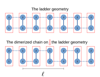
Figure 1: Weakly coupled dimer and two-leg ladder representation. The index $\eta$ corresponds for the ladder to the bottom or upper leg. For the dimer, $\eta$ corresponds to the left or right strong bond cell, thus the labels shuffle when mapped on the two-leg ladder geometry. We add an arrow on the middle cell to visualize the symmetry when we inverse the dimerized chain.

$$H_{\mathcal{L}}=J_{\parallel}\sum_{\ell,\eta}\mathbf{S}_{\ell,\eta}\cdot\mathbf{S}_{\ell+1,\eta}+J_{\perp}\sum_{\ell}\mathbf{S}_{\ell,1}\cdot\mathbf{S}_{\ell,2}-h^{z}\sum_{\ell,\eta}S^{z}_{\ell,\eta}$$ (1)

with stronger rung coupling where $\mathbf{S}_{\ell,\eta}$ denotes a spin-$1/2$ at rung $\ell$ on leg $\eta\in\{1,2\}$. The spin-$1/2$ $\mathbf{S}=(S^{x},S^{y},S^{z})=\frac{\hbar}{2}(\sigma^{1},\sigma^{2},\sigma^{3})$ can be decomposed in lowering and raising operators $S^{\pm}=S^{x}\pm iS^{y}$, where we denote by $\sigma^{i}$ the Pauli matrices, $i\in\{1,2,3\}$. Note that the coupling values are given in (4).

II.0.2 Dimer $\mathcal{D}$

If we remove alternatively the weak bonds along the ladder (see Fig. 1) and map the model to a chain we get a dimerized chain of alternative bonds. For an even number of sites $N$, we always have $\frac{N}{2}$ strong bonds $J_{s}$ and $\frac{N}{2}-1$ weak bonds $J_{w}$. The model is thus

$$H_{\mathcal{D}}=\sum_{n=1}^{N-1}(J-(-1)^{n}\delta J)\mathbf{S}_{n}\cdot\mathbf{S}_{n+1}-h^{z}\sum_{n=1}^{N}S^{z}_{n}$$ (2)

starting with a strong bond at each border $J_{s}=J+\delta J$ and alternating with the weak bonds $J_{w}=J-\delta J$ along the chain. The coupling values are given in (5).

II.0.3 Spin-Chain mapping - $\Delta=\frac{1}{2}$ XXZ chain $\mathcal{C}$

Both previous models can be mapped to an anisotropic single spin chain in some regime of parameters when studying the low-energy behaviorBouillot et al. (2011). If the magnetic field and temperature are such that we neglect the triplet $\left|t^{0}\right\rangle$ and $\left|t^{-}\right\rangle$ population, one can identify a spin-chain behavior in the critical interplay between $\left|t^{+}\right\rangle$ and $\left|s\right\rangle$.

We introduce the pseudo-spin-$1/2$ $\vec{\mathds{S}}$ in the basis $\left|\mathbin{\rotatebox[origin={c}]{90.0}{$\rightarrowtriangle$}}\right\rangle\equiv\left|t^{+}\right\rangle$, $\left|\mathbin{\rotatebox[origin={c}]{-90.0}{$\rightarrowtriangle$}}\right\rangle\equiv\left|s\right\rangle$ mapped by $S^{\pm}_{\eta}\equiv\frac{\eta}{\sqrt{2}}\mathds{S}^{\pm}$ and $S^{z}_{\eta}\equiv\frac{1}{4}\left(1+2\mathds{S}^{z}\right)$ in the singlet-triplet crossing region. The mapping leads to a spin-$1/2$ XXZ chain with $\Delta=\frac{1}{2}$ anisotropy

$$H_{\mathcal{C}}=J\sum_{\ell=1}^{N-1}\left(\mathds{S}^{x}_{\ell}\mathds{S}^{x}_{\ell+1}+\mathds{S}^{y}_{\ell}\mathds{S}^{y}_{\ell+1}+\frac{1}{2}\mathds{S}^{z}_{\ell}\mathds{S}^{z}_{\ell+1}\right)-h^{z}_{eff}\sum_{\ell=1}^{N}\mathds{S}^{z}_{\ell}$$ (3)

The spin-chain mapping fixes the following microscopic parameters for the XXZ model

1. ladder : $J\equiv J_{\parallel}$ and $h^{z}_{eff}=h^{z}-J_{\perp}-\frac{J_{\parallel}}{2}$,

2. dimer : $J\equiv\frac{-J_{w}}{2}$ and $h^{z}_{eff}=h^{z}-J_{s}-\frac{J_{w}}{4}$.

Although these models can be studied independently we consider them here in the regime where their low-energy properties are roughly equivalent. We consider spin chains close to zero magnetization $m_{\mathcal{C}}=0$, which means that both the two-leg ladder and the dimer are at a magnetization around half saturation $m_{\mathcal{L}}=0.5$ and $m_{\mathcal{D}}=0.25$ at $T=0$. We call this point in the paper the studied magnetic point for simplicity.

For the numerical study we fix the ratio of coupling constants of the ladder to values corresponding roughly to the compound BPCC Ward et al. (2013, 2017); Ryll et al. (2014); Tajiri et al. (2004) namely

$$\begin{split}J_{\parallel}&=0.39~{}J_{\perp}\\ J_{\perp}&=1\end{split}$$ (4)

In the same way for the dimer system we have

$$\begin{split}J_{w}&=J-\delta J=0.39~{}J_{s}\\ J_{s}&=J+\delta J=1\end{split}$$ (5)

The corresponding values for the magnetic field are respectively $h^{z}\simeq 1.28~{}J_{\perp}$ for the two-leg ladder and $h^{z}\simeq 1.148~{}J_{s}$ for the dimer. We will consider these values in the rest of the paper. We will not discuss the correction of the constant and the boundary terms in this paper.

One can see how the spin-chain mapping manifests on both models looking at Figs. 3 and 4 compared with Figs. 5 and 6.

III Method T-DMRG ($T\neq 0$)

We implement in this paper a time-dependent density-matrix renormalization group (T-DMRG) procedure Verstraete et al. (2004); Zwolak and Vidal (2004); Feiguin and White (2005); Barthel (2013), a method based on the earlier DMRG algorithm White (1992, 1993); Vidal (2003); Daley et al. (2004); Vidal (2004); White and Feiguin (2004); Schollwöck (2011).

The method is schematically represented in Fig. 2.

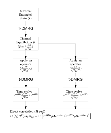
Figure 2: Simulation and measurement of direct correlations by evolving two observables in time to $t_{1}$ and $t_{2}$ at finite temperature using the T-DMRG algorithm. An optimal scheme, explained in Ref. Barthel, 2013, consists in evolving separately the two observables. This scheme requires storing all intermediate steps and contracting them at the end (see text). We use this scheme for the ladders since it can in principle double the resolution. The standard scheme consists in evolving only one observable in time ($t_{2}=0$) and in the present paper we use it both for the dimers and for the chains. Please note, that in our notation $\beta=2\tilde{\beta}$.

The time or imaginary time evolution follows the Suzuki-Trotter decompositionSuzuki (1991); McLachlan (1995). In this paper we used a fourth-order decomposition – that expands the exponentials in terms of gates which now can converge to the thermal equilibrium function $\frac{1}{Z}e^{-\beta H}$. One introduces hierarchical matrices for tensors that increase the amount of information stored in the system based on the local quantum numbersSingh et al. (2011); Hubig et al. (2017) and the global conservation rules.

Both DMRG and T-DMRG algorithm have the same complexity limit in term of the bond dimension $\chi$ of the matrices – during updates after application of above-mentioned gates. The singular value decomposition appears to scaleVidal (2004) as $O(\chi)\sim A\chi^{3}$ but with different prefactors $A$, which increases from $d^{3}$ for DMRG to $d^{6}$ for T-DMRG, where $d$ is the number of local degrees of freedom. A similar scaling applies to the memory case in which $O(\chi)\sim A\chi^{2}$ with $A\propto d^{2}$ for DMRG and $A\propto d^{4}$ for T-DMRG. For the case of ladders, due to the effective longer range of the couplings, if one represents the system as a chain, the gates have to be applied further which increases further the complexity. This is related to the fact that DMRG is most efficient for quantum problems with a sufficiently low amount of relevant informationEisert et al. (2010) and thus particularly for the low-dimensional problems.

III.1 T-DMRG and a close to optimal scheme

Since the complexities of the two-leg ladder and of the dimer are different due to the longer range of the coupling (see Fig. 1), one needs to restrict the bond dimension $\chi$ according to the problem. We use in this paper values of $\chi$ of the order of $\chi_{\mathcal{L}}\sim 620$ for the two-leg ladders and $\chi_{\mathcal{D}}\sim 2400$ for the dimers.

With the values of $\chi_{\mathcal{L}}$ for the two-leg ladders, the use of the standard scheme Barthel (2013); Coira et al. (2018) of implementation of the time and temperature evolution does not allow us to reach sufficiently long time and resolution for the ladder case. This happens even though the dimers and the two-leg ladders appear to be quite similar. Thus, in order to be able to study reliably the two-leg ladders we have implemented an optimal numerical scheme as described in Ref. Barthel, 2013 (see Fig. 2), which was only scarcely used in the literature previously due to its more demanding implementation. As shown in Fig. 2, the usual procedure evolves only one observable in time, while the optimal scheme consists of evolving both operators in time. In practice, this requires only a logistic approach (storing of the state) and running the jobs in parallelTange (2015). However, due to hardware limits, it is in practice difficult to store all the states and parallelize the contraction properly.

We use the optimal scheme for the two-leg ladder case to increase the resolution of Fig. 3 and Fig. 4. For the other models, we use the normal scheme consisting of evolving only one observable in time (Fig. 2 with $t_{2}=0$).

We compute the spin-spin correlations in space and time

$$\left\langle S^{\alpha}_{x_{0}}(t)S^{\gamma}_{x_{1}}\right\rangle_{\beta}$$ (6)

for positive time $t\geq 0$ and fixed observable at $x_{0}$. We detail in Sec. IV how we Fourier transform the measured correlations. We compute these correlations for various temperatures as given in Table 1.

Table 1: Temperatures presented in Figs. 3–12 and 14. All the results are given at the studied magnetic point in the middle of the critical gapless phase.

Model	Figure	Temperature
ladder $\mathcal{L}$	Fig. 3	$T=0.25~{}J_{\perp}\simeq 0.64~{}J_{\parallel}$
	Fig. 4	$T=0.595~{}J_{\perp}\simeq 1.526~{}J_{\parallel}$
$\leftharpoonup$ slices (Sec.V) $\rightarrow$	Fig. 12	$0.64~{}J_{\parallel}\lesssim T\lesssim 1.526~{}J_{\parallel}$
dimer $\mathcal{D}$	Fig. 5	$T=0.25~{}J_{s}\simeq 1.28~{}J_{w}/2$
	Fig. 6	$T=0.595~{}J_{s}\simeq 3.05~{}J_{w}/2$
	Fig. 14	$T=0.05~{}J_{s}\simeq 0.26~{}J_{w}/2$
$\leftharpoonup$ $t^{0}$ excitation  $\rightarrow$	Figs. 8,9	$0.05~{}J_{s}\lesssim T\lesssim 0.595~{}J_{s}$
$\leftharpoonup$ slices (Sec.V) $\rightarrow$	Fig. 11	$0.26~{}J_{w}/2\lesssim T\lesssim 3.05~{}J_{w}/2$
chain $\mathcal{C}$	Fig. 7	$T=0.25~{}J$
$\leftharpoonup$ slices (Sec.V) $\rightarrow$	Fig. 10	$0.1~{}J\lesssim T\lesssim 3.05~{}J$

III.2 Simulation accuracy

Comparing the initial DMRG version with the finite temperature algorithm, one sees that the variance of the Hamiltonian $\left\langle\left(H-\left\langle H\right\rangle\right)^{2}\right\rangle$ is now finite and no longer a criterion for convergence. To define the convergence of the calculation, we use the discarded weight quantityBarthel (2013), namely the total weight of discarded eigenvalues according to the singular value $\lambda_{j}$ decomposition.

$$\epsilon_{i}\equiv\left(\frac{\left\lVert X_{\scriptsize\text{trunc}}-X\right\rVert}{\left\lVert X\right\rVert}\right)^{2}=\frac{\sum_{j>\chi}\lambda_{j}^{2}}{\sum_{j}\lambda_{j}^{2}}$$ (7)

where $i$ can denote the inverse temperature $\beta$, the time $t$ or a single step process depending on the context. The sum applies in all quantum sector blocks. $X$ is in the matrix product operatorVerstraete et al. (2004) form and $X_{\scriptsize\text{trunc}}$ is the truncated matrix product approximation with the renormalized bond dimension fixed to $\chi$.

The norm can be viewed as the Frobenius normBarthel (2013). $\chi$ is the bond dimension of the mixed state, and corresponds to the number of states kept in the system. This discarded weight quantity is a good indicator of the T-DMRG algorithm precision (see Appendix A).

III.2.1 Ladders $\mathcal{L}$

For the two-leg ladder, we fixed the size to a total of $2\cdot 45=90$ ladder sites. The run uses a truncation error $\epsilon_{\beta}=10^{-18}$ and steps in imaginary time $\delta\beta=\frac{1}{100}$ to converge to the thermal equilibrium $\beta=4.0~{}J_{\perp}^{-1}$, $3.04~{}J_{\perp}^{-1}$ and $1.68~{}J_{\perp}^{-1}$ which are the three temperatures considered for the ladders in the present paper.

The initial bond dimension $\chi_{\beta}<800$ remains largely controlled (it did not reach the limit size $800$) in this initial step since the temperatures are quite large. Then we fix for all the different observables the truncation $\epsilon_{t}=10^{-13}$, $\delta t=\frac{1}{16}$ and bond dimension $\chi_{t}=620$. Typically the amount of information in the time simulation grows until the maximal bond dimension is reached. Then, one loses a precision of $\epsilon_{i}$ at each step by discarding the smallest singular values $\lambda_{j}$ according to (7), which is mandatory if one wants to keep the numerical algorithmic complexity size $\chi$ of the matrices fixed. The algorithm stops when the total discarded weight passes a threshold $\sum_{i\in\{\text{all steps}\}}\epsilon_{i}>10^{-2}$ or when a single step lacks in precision $\epsilon_{i}>10^{-5}$.

The above precision is for the middle site observable (left column of Fig. 2). All the other observables run in parallel with the same time algorithm procedure (or half the sites using afterwards the symmetry along the ladder). In order to be sufficiently fast, we reduce the bond dimension $\chi_{t}=400$ as well as the final time $t_{2}\sim 7-8~{}J_{\perp}^{-1}$ to ensure a precision $\epsilon_{t}\lesssim 10^{-7}$. We can then compute the direct correlations in Fig. 2 with $t_{1}$ up to $19-23~{}J_{\perp}^{-1}$ (time within the bulk without encountered borders) and we find a good overlap between all different time correlations – it gets a bit worse for values of $t_{1}$ close to the maximal reachable time as expected. This optimal scheme brings an increase in time $t=\left|t_{1}\right|+\left|t_{2}\right|$ or a resolution improvement of $\sim 30-50\%$ in the worst or best scenario.

III.2.2 Dimers $\mathcal{D}$

For the dimer case, we get a similar resolution in $J_{s}$ without using the optimal scheme for $L=90$ sites. We first converge with the truncation error $\epsilon_{\beta}=10^{-18}$ with steps $\delta\beta=\frac{1}{100}$ to the thermal equilibrium at $\beta=20~{}J_{\perp}^{-1}$, $10~{}J_{\perp}^{-1}$, $4.0~{}J_{\perp}^{-1}$, $1.68~{}J_{\perp}^{-1}$. One then fixes all the different observables and time evolves by $\delta t=\frac{1}{16}$ with the truncation $\epsilon_{t}=10^{-13}$ with the limited bond $\chi_{t}=2400$. The simulation stops again according to the same threshold and the final times are for the high temperatures of order $t_{\text{max}}\sim 27-58~{}J_{\perp}^{-1}$. For a lower temperature $T\ll J_{w}$, one can achieve a better resolution similar to standard DMRG results (see Ref. Coira et al., 2018).

IV Correlations for ladders, dimers and chains

IV.1 Dynamical structure factor

We first need to transform the real-time and -space data to find the dynamical structure factor.

$$S^{\alpha\gamma}(\mathbf{q},\omega)=\int_{-\infty}^{\infty}\!\mathrm{d}\mathbf{r}\,\mathrm{d}t\,\mathrm{e}^{i(\omega t-\mathbf{q}\cdot\mathbf{r})}\langle{S}^{\alpha}(\mathbf{r},t){S}^{\gamma}(0,0)\rangle$$ (8)

In the following equations, $\alpha,\gamma\in\{x,y,z,\pm\}$ denote any component of the spin-$1/2$.

The T-DMRG simulation gives the direct correlations $\left\langle S^{\alpha}_{x_{0}}(t)S^{\gamma}_{x_{1}}\right\rangle_{\beta}$ restricted to positive time $t\geq 0$. In order to avoid making errors using spatial invariance too early (before time inversion which can be critical for dimers) we use the retarded susceptibility to ensure an exact procedure. Although this sounds a priori more complicated, it actually becomes more straightforward since the time symmetry is carried by the Kramers-Kronig relations. Furthermore, the $S^{z}$ sector of the spin does not need the average magnetization – hidden in the real part – to calculate the connected correlation.

IV.1.1 Chains $\mathcal{C}$

We illustrate this procedure for the spin chain. We first Fourier transform in time the retarded susceptibility that we get by expressing it in a function of our direct correlations

$$\chi^{\alpha\gamma}_{\text{ret}}(\omega,x_{0},x_{1})=\int dt\;e^{+i(\omega+i\varepsilon)t}(-i\Theta(t))\left\langle\left[S^{\alpha}_{x_{0}}(t),S^{\gamma}_{x_{1}}\right]\right\rangle$$

$$=-i\int_{0}^{+\infty}dte^{+i(\omega+i\varepsilon)t}\left(\left\langle S^{\alpha}_{x_{0}}(t)S^{\gamma}_{x_{1}}\right\rangle-\overline{\left\langle S^{\alpha\dagger}_{x_{0}}(t)S^{\gamma\dagger}_{x_{1}}\right\rangle}\right)$$

where $\overline{\left\langle\dots\right\rangle}$ denotes complex number conjugation and $S^{\pm\dagger}_{x_{0}}=S^{\mp}_{x_{0}}$. We then use translation invariance $x=x_{1}-x_{0}$ in the bulk and Fourier transform the space

$$\chi^{\alpha\gamma}_{\text{ret}}(q,\omega)=\int dx\;e^{-iqx}\chi^{\alpha\gamma}_{\text{ret}}(\omega,x)$$

to finally get the dynamical structure factor worked out using the Lehmann representation

$$S^{\alpha\gamma}(q,\omega)=\frac{-2}{1-e^{-\beta\omega}}\operatorname{Im}\left(\chi_{\text{ret}}^{\alpha\gamma}(q,\omega)\right)$$

The detail of this equality can be found in Appendix B.

IV.1.2 Ladders $\mathcal{L}$

For the ladder, we have two species of correlations according to the leg index $\eta\in\{1,2\}$. We use the $q_{\perp}$ momentum to represent the correlations since it is a good quantum number. Thereby the observables and correlations separate in the symmetric $q_{\perp}=0$ or antisymmetric $q_{\perp}=\pi$ sectors. We use the following definitions

$$S^{\alpha}_{\ell,q_{\perp}=0} \equiv S^{\alpha}_{\ell,1}+S^{\alpha}_{\ell,2}$$

$$S^{\alpha}_{\ell,q_{\perp}=\pi} \equiv S^{\alpha}_{\ell,1}-S^{\alpha}_{\ell,2}$$

and calculate the dynamical structure factor from there. The two correlations are fully represented in the two $q_{\perp}$ quantum sectors

$$\left\langle S^{\alpha}_{q_{\perp}}(q,\omega)S^{\gamma}_{q_{\perp}}\right\rangle=2\left(\left\langle S^{\alpha}_{1}(q,\omega)S^{\gamma}_{1}\right\rangle\pm\left\langle S^{\alpha}_{1}(q,\omega)S^{\gamma}_{2}\right\rangle\right)$$

where the index corresponds to correlations on the same legs or, respectively, different legs. The symmetric $q_{\perp}=0$ case corresponds to the sum while the antisymmetric $q_{\perp}=\pi$ case is the difference. Using the rung symmetry, all other mixtures vanish, $\left\langle S^{\alpha}_{q_{\perp}=0}(q,\omega)S^{\gamma}_{q_{\perp}=\pi}\right\rangle=0$.

IV.1.3 Dimers $\mathcal{D}$

Dimers have less symmetry than the two-leg ladder. One can map the dimer on the ladder structure, but $q_{\perp}$ is not a good quantum number anymore. This can be seen for the $\left\langle S^{\alpha}_{\ell,1}S^{\gamma}_{0,2}\right\rangle$ correlation, which is not symmetric by space inversion anymore – in contrast to the ladder case (see Appendix C). In one direction the correlation starts with a weak bond while in the other direction it starts with a strong bond. However, we can map the dimer on the ladder by introducing similar definitions

$$S^{\alpha}_{\ell,q_{\perp}=0} \equiv(S^{\alpha}_{\ell,1}+S^{\alpha}_{\ell,2})$$

$$S^{\alpha}_{\ell,q_{\perp}=\pi} \equiv(S^{\alpha}_{\ell,1}-S^{\alpha}_{\ell,2})(-1)^{\ell}$$

The new ladder labeling introduces the oscillating sign according to Fig. 1 while the symmetric observable $S^{\alpha}_{\ell,q_{\perp}=0}$ remains untouched by the permutation. Note that the crossed correlations $\left\langle S^{\alpha}_{q_{\perp}=0}(q,\omega)S^{\gamma}_{q_{\perp}=\pi}\right\rangle\neq 0$ are not vanishing but not very transparent to analyze. We thus focus on the correlations

$$\left\langle S^{\alpha}_{q_{\perp}=0}(q,\omega)S^{\gamma}_{q_{\perp}=0}\right\rangle$$

$$\left\langle S^{\alpha}_{q_{\perp}=\pi}(q,\omega)S^{\gamma}_{q_{\perp}=\pi}\right\rangle$$

These correlations look similar to the two-leg ladder up to finite signal strength absent in the ladders as can be seen in Fig. 5 and Fig. 6.

For completeness, we also present in Appendix D (Fig. 14) the results in the more conventional chain notation in which we separate the correlations in $\left\langle S^{\alpha}_{1}(q,\omega)S^{\gamma}_{1}\right\rangle$ and $\left\langle S^{\alpha}_{1}(q,\omega)S^{\gamma}_{2}\right\rangle$, which are now two-site cell translation invariant.

IV.1.4 Filter

In the previous paragraph, we made major assumptions such as translation invariance and infinite time integration. Respectively, we then should expect errors of the order $\Delta q=\frac{\pi}{d_{max}}$ and $\Delta\omega=\frac{\pi}{t_{max}}$ inside each Fourier transformation due to finite-size effects. As usual, the most relevant error comes from the real-time resolution which is much harder to get. In order to remove finite-size effects on our data and give more weight to the short space and time steps, one can introduce a selective mask.

In the first part (Sec. IV.2), we add a weak Gaussian filter $M(x,t)=e^{-(Ax/d_{max})^{2}}e^{-(Bt/t_{max})^{2}}$ where we choose $A=B=1.5$.

In the second part (Sec. V), where we compare the results with the field theory expectation, we avoid all filters and work with the raw correlations.

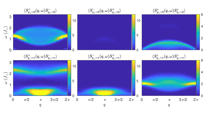
Figure 3: Spin-spin correlations of a spin-$1/2$ two-leg ladder in units of $J_{\perp}=1$ with $J_{\parallel}=0.39~{}J_{\perp}$ at $T=0.25~{}J_{\perp}\simeq 0.64~{}J_{\parallel}$ for magnetic field $h^{z}=1.28~{}J_{\perp}$ corresponding to $m_{\mathcal{L}}\simeq 0.5$. The resolution is $\Delta\omega=\frac{\pi}{30~{}J_{\perp}^{-1}}$ using the optimal scheme.

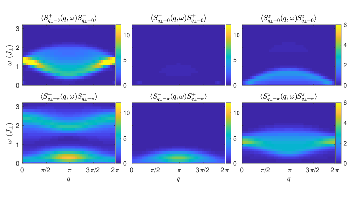
Figure 4: Spin-spin correlations of a spin-$1/2$ two-leg ladder in units of $J_{\perp}=1$ with $J_{\parallel}=0.39~{}J_{\perp}$ and at $T=0.595~{}J_{\perp}\simeq 1.526~{}J_{\parallel}$ for magnetic field $h^{z}=1.28~{}J_{\perp}$ corresponding to $m_{\mathcal{L}}\simeq 0.5$. The resolution is $\Delta\omega=\frac{\pi}{22.5~{}J_{\perp}^{-1}}$ using the optimal scheme.

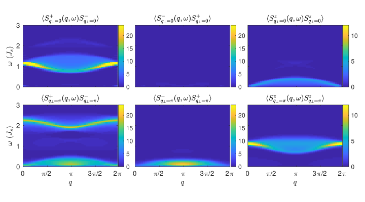
Figure 5: Weakly coupled dimerized chain in units of $J_{s}=1$ with $J_{w}=0.39~{}J_{s}$ at $T=0.25~{}J_{s}\simeq 1.28~{}J_{w}/2$ for magnetic field $h^{z}=1.148~{}J_{s}$ corresponding to $m_{\mathcal{D}}\simeq 0.25$. The resolution is $\Delta\omega=\frac{\pi}{35~{}J_{s}^{-1}}$ using the standard scheme.

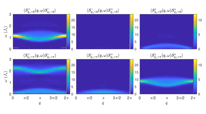
Figure 6: Weakly coupled dimerized chain in units of $J_{s}=1$ with $J_{w}=0.39~{}J_{s}$ at $T=0.595~{}J_{s}\simeq 3.05~{}J_{w}/2$ for magnetic field $h^{z}=1.148~{}J_{s}$ corresponding to $m_{\mathcal{D}}\simeq 0.25$. The resolution is $\Delta\omega=\frac{\pi}{27~{}J_{s}^{-1}}$ using the standard scheme.

IV.2 Results for the correlation functions

Let us now present the results based on the calculations described in the previous sections.

The central results of this section are the calculation of the correlation functions for the ladders at finite temperature. Results for the two-leg ladder model (1) are presented in Fig. 3 for a temperature of $T=0.25~{}J_{\perp}$ and in Fig. 4 for temperature $T=0.595~{}J_{\perp}$. Previous results but at zero temperature $T=0$ can be found in Ref. Bouillot et al., 2011.

All allowed transitions for an isolated rung can be found in Table 2 for the symmetric and antisymmetric spin observables. Briefly we review the different excitations that appear in the two-leg strong rung ladder, and we will discuss it further in the next sections. In the gapless phase, the lowest excitation spectrum is of course due to the interplay of the singlets with the triplets forming the Descloizeaux-Pearson continuum spectrum (see Sec. V for a finer study of the low spectrum behavior and Fig. 7). At intermediate energy, one sees the dispersion of a single triplet excitation $\left|t^{0}\right\rangle$ in the correlations $\left\langle S^{+-}_{q_{\perp}=0}\right\rangle$ and $\left\langle S^{zz}_{q_{\perp}=\pi}\right\rangle$ (see the $t-J$ modelBouillot et al. (2011) which breaks down here at finite $T\neq 0$, see Fig. 8). In addition to the same energy scale, there is a weak two-triplet excitation signal in $\left\langle S^{-+}_{q_{\perp}=0}\right\rangle$. At large energy scale, one encounters another weak two-triplet excitation in the $\left\langle S^{zz}_{q_{\perp}=0}\right\rangle$ as well as a transition to the single triplet $\left|t^{-}\right\rangle$ excitation in the $\left\langle S^{+-}_{q_{\perp}=\pi}\right\rangle$.

Table 2: Transition elements of the symmetric and antisymmetric spin-$1/2$ operator $\left\langle\cdot\right|S^{\alpha}_{q_{\perp}}\left|\cdot\right\rangle$ in the isolated rung picture. According to the Lehmann representation (see Appendix B), all above-mentioned spectra can be identified by the following transitions.

$\mathbin{\rotatebox[origin={c}]{55.0}{$\left\langle S^{\alpha}_{q_{\perp}}\right\rangle$}}$	$\left|s\right\rangle$	$\left|t^{+}\right\rangle$	$\left|t^{0}\right\rangle$	$\left|t^{-}\right\rangle$
$\left\langle s\right|$	$\emptyset$	$\scriptstyle\left\langle S^{-}_{\pi}\right\rangle=-\sqrt{2}$	$\scriptstyle\left\langle S^{z}_{\pi}\right\rangle=1.0$	$\scriptstyle\left\langle S^{+}_{\pi}\right\rangle=\sqrt{2}$
$\left\langle t^{+}\right|$	$\scriptstyle\left\langle S^{+}_{\pi}\right\rangle=-\sqrt{2}$	$\scriptstyle\left\langle S^{z}_{0}\right\rangle=1.0$	$\scriptstyle\left\langle S^{+}_{0}\right\rangle=\sqrt{2}$	$\emptyset$
$\left\langle t^{0}\right|$	$\scriptstyle\left\langle S^{z}_{\pi}\right\rangle=1.0$	$\scriptstyle\left\langle S^{-}_{0}\right\rangle=\sqrt{2}$	$\emptyset$	$\scriptstyle\left\langle S^{+}_{0}\right\rangle=\sqrt{2}$
$\left\langle t^{-}\right|$	$\scriptstyle\left\langle S^{-}_{\pi}\right\rangle=\sqrt{2}$	$\emptyset$	$\scriptstyle\left\langle S^{-}_{0}\right\rangle=\sqrt{2}$	$\scriptstyle\left\langle S^{z}_{0}\right\rangle=-1$

In the same way, and in order to be able to compare with the ladder results, we present the finite temperature correlations for the dimerized system. Similar calculations, albeit at different temperatures and couplings, were given in Ref. Coira et al., 2018. The comparison of the results of the present paper with the results of Ref. Coira et al., 2018 for the correlation $\left\langle S_{1}^{\alpha}S_{1}^{\gamma}\right\rangle_{\beta}$ in the gapless phase is very good. We find similar limitations during the time evolution process for the most cumbersome $\frac{e^{-\beta H}}{Z}S^{+}$ observable and similar improvement of resolution when lowering the temperature.

The dimerized system mapped on the ladder geometry is shown in Fig. 5 at a temperature $T=0.25~{}J_{s}$ and in Fig. 6 for a temperature $T=0.595~{}J_{s}$. As one can see, most of the excitations can be identified with the two-leg ladder pretty well.

Finally we also present the results for the chains at similar temperatures in Fig. 7. Finite temperature calculations of spin chains were also presented in Ref. Barthel et al., 2009.

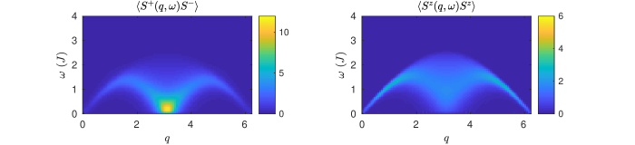
Figure 7: XXZ spin-$1/2$ chain with anisotropy $\Delta=\frac{1}{2}$ and coupling $J=1$ at $T=0.25~{}J$ for an external magnetic field $h=0~{}J$ corresponding to a zero magnetization $m_{\mathcal{C}}=0$. The resolution is $\Delta\omega=\frac{\pi}{52~{}J^{-1}}$.

IV.3 Discussion of the T-DMRG results

First let us note that the weights in the correlations redistribute differently than for the zero-temperature caseBouillot et al. (2011). Due to the finite temperature effects, some negative energy transitions are allowed in the correlations (see Fig. 14). We only present the results for the positive frequency domain $\omega\geq 0$ since one can relate them to the negative frequencies using the detailed balance equation (17)

$$S^{\alpha\gamma}(q,\omega)=e^{-\beta\omega}S^{\gamma\alpha}(-q,-\omega)$$ (9)

Since the raising and lowering are not self-conjugate operators, they are allowed at finite temperature to get negative intensities (see Fig. 14).

Even though the natures of the correlations are quite different due to the different species of correlations, ladders and dimers are quite related and give good information on each other. There are indeed many similarities in the structure factors. The triplets are quite well aligned in energy. One difference that can be directly seen in the numerical results but will be deepened using the mapping onto an effective spin chain (see Sec. V.3) is that the dimer has an effective dispersion of $J_{w}/2$ compared to $J_{\parallel}$ for the two-leg ladder. All quantities depending on the weak bonds thus rescale for the dimer by a factor of $2$. For this reason, we use a twice larger colorbar color code for the dimer than the ladder to represent the intensities on a similar scale – but all presented results stay in unity of $J_{s}$ and $J_{\perp}$. In addition, due to the asymmetry of the dimer, some signals survive in the region where the ladder is actually gapped (correlations in $q_{\perp}=0$ and $q_{\perp}=\pi$ are not allowed between the $\left|t^{+}\right\rangle$ and $\left|t^{0}\right\rangle$ or $\left|t^{0}\right\rangle$ and $\left|t^{-}\right\rangle$). This is a remnant of the different types of geometries and the absence of “ladder-like” symmetries in the dimer case (see Appendix C). In addition to that, the weak two-triplet $\left\langle S^{-+}_{q_{\perp}=0}\right\rangle$ at intermediate energy scale is absent in the dimerized chain.

Concerning the effective temperature in each model, the two-leg ladder remains more coherent in the low-energy spectrum than the dimer since it “feels” a twice smaller temperature in units of the effective dispersion. We discuss the low spectrum in more details in the next section (Sec. V) by comparing the results with field theory predictions.

Let us now turn to the higher part of the energy spectrum. This part of the spectrum is of course beyond the reach of the field theory and the mapping onto the anisotropic spin chain. As a general tendency we get weaker intensities and more spread signals when the temperature increases. The temperature leads also to a broadening of the modes, that was analyzed for the dimers from the numerical resultsCoira et al. (2018). We see here that the ladders show similar behaviors in term of broadening (see Figs. 3 and 4). We concentrate here on the spectrum corresponding to an excitation to the state $\left|t^{0}\right\rangle$ and study in detail its temperature dependence, in particular for the same order or larger temperature than the weak coupling (see Fig. 8). For both ladders and dimers, this part of the spectrum corresponds to modes in which a singlet or a $\left|t^{+}\right\rangle$ state is converted into a $\left|t^{0}\right\rangle$. One can thus examine this part of the spectrum as a single hole in a $t-J$ model Bouillot et al. (2011) for which the “hole” corresponds to the state $\left|t^{0}\right\rangle$ and the two “spin” states are played by the singlet and $\left|t^{+}\right\rangle$ states. At low (or zero) temperature as was clearly shown both for ladders at zero temperature (see Figs. 12,13 in Bouillot et al., 2011) and for dimers (see Figs. 11,12 in Coira et al., 2018) (note that the antisymmetric signal $q_{\perp}=\pi$ is shifted by $\pi$ in our results compared to the chain (in agreement with our Fig. 14)), the spectrum corresponds to two cosine dispersions centered around the two minima $q=\pi/2$ and $q=3\pi/2$ because the creation of a $\left|t^{0}\right\rangle$ state is accompanied by the destruction of either a singlet $\left|s\right\rangle$ or a triplet $\left|t^{+}\right\rangle$ (see Sec. V.C.3.b in Bouillot et al., 2011). At the magnetic field we have applied, the low part of the excited spectrum corresponds to the low-energy states $\left|t^{+}\right\rangle$ and $\left|s\right\rangle$ with momentum for the excitations of $q=\pm\pi/2$ at half filling.

From our numerical results we can follow the dispersion of the $\left|t^{0}\right\rangle$ mode as the temperature increases from temperatures small to large compared to the effective dispersion. The results are shown in Fig. 8.

The lower temperature is clearly in agreement with the previous results both for the dimers and for the ladders with the dispersion minima around $\pi/2$ and $3\pi/2$ resulting from the mapping to an effective $t-J$ model. As the temperature increases we see that the modes become increasingly incoherent and broaden. Quite surprisingly the numerical result shows that the dispersion leads to a relevant intensity corresponding to a coherent like mode, with its maximum intensity at the bottom of the spectrum, with a minimum which is now shifted to around $q\sim\pi$. This behavior is observed for the dimers as shown in Figs. 8 and 9, but also for ladders as can be seen from Fig. 4. Giving a precise description of this effective “mode” is an interesting and challenging question since it originally appears from the many-body dynamics. An interesting challenge would be finding the temperature for which the incoherent minimal peak would become maximal.

Although it is difficult to connect this observation directly to an analytical calculation, one can infer that the change of the spectrum comes from the fact that the spinon excitations that would correspond to the two pseudo-spin singlet $\left|s\right\rangle$ and triplet $\left|t^{+}\right\rangle$ states are now essentially totally incoherent since the temperature is greater than their dispersion, leading to essentially the dispersion of the bare hole.

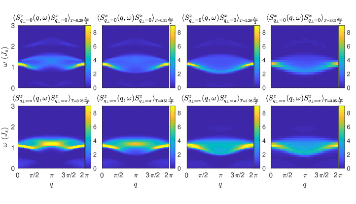
Figure 8: The single triplet excitation $t^{0}$ in weakly coupled dimerized chain in units of $J_{s}=1$ with $J_{w}=0.39~{}J_{s}$ at magnetic field $h^{z}=1.148~{}J_{s}$ corresponding to $m_{\mathcal{D}}\simeq 0.25$ for various temperature $T=0.05,\,0.1,\,0.25,\,0.595~{}(J_{s})$. The last two columns corresponds to top left and bottom right panels of Figs. 5 and 6. At the lowest temperatures we see that the minima of the dispersion are situated around $q=\pi/2$ and $q=3\pi/2$ in agreement with the predictions of the mapping of this system to a $t-J$ model Bouillot et al. (2011). When the temperature increases and becomes larger than $J_{w}$ one sees that a coherent-like mode with a minimum around $q=\pi$ appears at the bottom of the spectrum in an incoherent background (see text and Fig. 9).

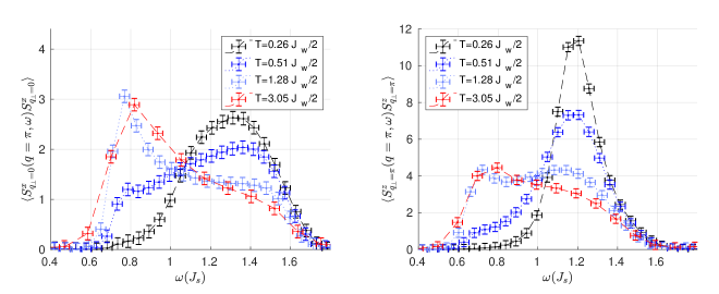
Figure 9: Slice at $q=\pi$ of Fig. 8 focusing on the energy range of the $\left|t^{0}\right\rangle$ excitation for the correlations $\left\langle S^{x}_{q_{\perp}=0}(q=\pi)S^{x}_{q_{\perp}=0}\right\rangle$ on the left and $\left\langle S^{z}_{q_{\perp}=\pi}(q=\pi)S^{z}_{q_{\perp}=\pi}\right\rangle$ on the right. We see a shift of the spectral weight there moving the mode from $1.2-1.4~{}J_{s}$ at low temperature to $0.7-0.85~{}J_{s}$ at large temperature. This complex mechanism appears to arise from the many-body dynamics and breaks the usual low-temperature picture done by the $t-J$ mappingBouillot et al. (2011).

V Comparison with field theory

Let us now turn to the low-energy part of the spectra. Both the two-leg ladder and the dimer system can be mappedBouillot et al. (2011); Coira et al. (2018) at the studied magnetic point to an anisotropic spin-$1/2$ $\Delta=\frac{1}{2}$ XXZ model. This allows us to use the standard bosonization method to extract the dynamical correlation functions Giamarchi (2003) both at zero temperature, and using the conformal invariance of the field theory, at low temperature. In a similar way to what was done for the NMR relaxation time Coira et al. (2016) one can thus compare the numerical results with the field theory description.

V.1 Bosonization of the spin-$1/2$ chain

Let us give a brief reminder of the field theory description. One introducesGiamarchi (2003) two continuous real bosonic fields $\phi$ and $\theta$ to represent the low-energy excitations. For an XXZ spin chain, the effective Hamiltonian is

$$H=\frac{\hbar}{2\pi}\int\,dx\frac{uK}{\hbar^{2}}(\nabla\theta(x))^{2}+\frac{u}{K}(\nabla\phi(x))^{2}$$ (10)

where $u$ is the velocity of excitations and $K$ is a dimensionless parameter, controlling the decay of the correlation functions. The spin operators are represented in terms of the fields $\phi$ and $\theta$ byGiamarchi (2003)

$$S^{z}(\mathbf{r}) =m_{z}+\frac{-1}{\pi}\nabla\phi(\mathbf{r})+\frac{2}{2\pi\alpha}\cos(2\phi(\mathbf{r})-\pi(1+2m_{z})x)$$

$$S^{\pm}(\mathbf{r}) =\frac{e^{\mp i\theta(\mathbf{r})}}{\sqrt{2\pi\alpha}}\left(\cos(\pi x)+\cos(2\phi(\mathbf{r})-2\pi m_{z}x)\right)$$ (11)

where $m_{z}$ is the magnetization.

For ladders and dimerized chains, we use the spin-chain mapping described in Sec. II.0.3 to relate the observables to the ones of a spin chain.

$$\begin{split}\mathds{S}^{z}_{l}\;&=2S^{z}_{l,k}-\frac{1}{2}\\ \mathds{S}^{\pm}_{l}&=(-1)^{k}\sqrt{2}~{}S^{\pm}_{l,k}\end{split}$$ (12)

The spin-spin correlation functions are given in the retarded susceptibility form bySchulz and Bourbonnais (1983); Chitra and Giamarchi (1997); Giamarchi (2003)

$$\chi_{\kappa}(\breve{q},\omega)=-\frac{\sin(\pi\kappa)\alpha^{2}}{u}\left(\frac{2\pi\alpha}{\beta u}\right)^{2\kappa-2}\text{B}\left(\frac{\kappa}{2}-i\frac{\beta(\omega-u\breve{q}+i\varepsilon)}{4\pi},1-\kappa\right)\text{B}\left(\frac{\kappa}{2}-i\frac{\beta(\omega+u\breve{q}+i\varepsilon)}{4\pi},1-\kappa\right)$$ (13)

where $\beta$ is the inverse temperature, $\alpha$ is a short distance cutoff, and $\breve{q}$ is the momentum centered on the field-dependent dispersion (the usual momentum $q$ is defined in Sec. IV.1.1). $\kappa$ is an exponent that depends on the precise correlation function under consideration. In this paper we look at the studied magnetic point and at slices at $q=\pi\pm 0.14$ (note that we are slightly above half saturation too), which would correspond to the $\breve{q}=0$ slice with TLL exponents $2\kappa=2K$ or $2\kappa=\frac{1}{2K}$ according to equation (14).

The non-universal parameters of the field theory (TLL parameters and amplitudes for the correlation functions) can be computed directly allowing an essentially parameter free calculation of the correlation functions. For the spin chain with $\Delta=\frac{1}{2}$, exact Bethe-Ansatz results Giamarchi and Tsvelik (1999) fix $K=0.75$ and $u=1.299$. However, for the two-leg ladder and the dimer those parameters need to be fixed from a numerical calculation with the microscopic model.

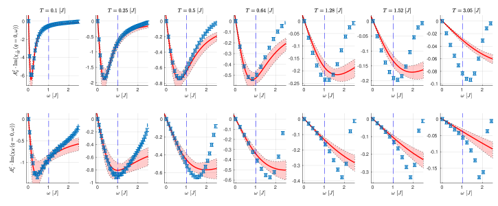
Figure 10: Transverse (top) and longitudinal (bottom) spin-spin correlation functions for a spin-$1/2$ chain as a function of the frequency $\omega$ for a fixed wave vector $q=\pi$ and $\breve{q}=0$, respectively (see Eq. (14)). The field theory expression (13) in red is directly compared with the numerical T-DMRG calculation of the correlation (blue). The numerics are obtained from the Fourier transform of the output simulation without Gaussian filter (Sec. IV.1.4). We have taken $A_{x}^{\mathcal{C}}\simeq 0.135$, $A_{z}^{\mathcal{C}}\simeq 0.09$, and $K^{\mathcal{C}}\simeq 0.745$. The shadow region corresponds to the maximum and minimum of all TLL parameters moving by $\pm 10\%$.

V.2 Extraction of TLL parameters at $T=0$

Table 3: TLL parameters extracted from $T=0$ DMRG data for the chain, dimer, and two-leg ladder systems. In italic in row $A_{z}$, $A^{\mathcal{C}}_{z}$ could not be extracted directly from the DMRG but has been fixed between the chain and the ladder (see text).

TLL parameters	chain $\mathcal{C}$	dimer $\mathcal{D}$	ladder $\mathcal{L}$
$A_{x}$	$0.135$	$0.1469$	$0.166$
$B_{x}$	$0.021$	$0.0135$	$0.007$
$A_{z}$	$0.09$	$\mathit{0.082}$	$0.078$
$K$	$0.745$	$0.754$	$0.85$

In order to fix the various parameters we use the expression of the correlation functions at zero temperatureGiamarchi (2003)

$$\left\langle S^{x}_{i}S^{x}_{j}\right\rangle =(-1)^{|i-j|}A_{x}\left(\frac{1}{{|i-j|}}\right)^{\frac{1}{2K}}-B_{x}\left(\frac{1}{{|i-j|}}\right)^{2K+\frac{1}{2K}}$$

$$\left\langle\delta S^{z}_{i}\delta S^{z}_{j}\right\rangle =\frac{-K}{2\pi^{2}}\left(\frac{1}{{|i-j|}}\right)^{2}+A_{z}(-1)^{|i-j|}\left(\frac{1}{{|i-j|}}\right)^{2K}$$

These expressions can then be used, by comparison with the numerical results, to extract Hikihara and Furusaki (2001); Bouillot et al. (2011) the non-universal amplitudes $A_{x}$, $B_{x}$, and $A_{z}$ and the $K$ parameter. We perform the zero-temperature DMRG calculation of the correlation functions using the ALPS libraryDolfi et al. (2014).

We first extracted the $A_{x}$ and $K$ parameter from the $\left\langle S^{x}_{i}S^{x}_{j}\right\rangle$ correlation since it has the slowest decay. We then use the obtained value of $K$ in the $\left\langle S^{z}_{i}S^{z}_{j}\right\rangle$ correlation and fix $A_{z}$. We avoid boundary effects by considering correlations near the middle of the chain and by using space invariance for few sites in the bulk. With this procedure, we estimate all errors on the extracted values of about $20\%$. The velocity $u$ is computed from the compressibility $\frac{K}{u\pi}=\frac{\partial m}{\partial h}$. In this paper we used $u\simeq 1.3$. The TLL values can be found in the table 3 and are consistent when they can be compared with previous resultsHikihara and Furusaki (2001); Bouillot et al. (2011).

For the dimer system, it is more difficult than for the chain and the ladder to extract the TLL parameters. For instance, the $\left\langle S^{z}_{i}S^{z}_{j}\right\rangle$ correlation decreases very fast while on the other hand the local magnetization still oscillates. With the asymmetry in the correlation, it becomes difficult to extract from there any estimation of $A^{\mathcal{D}}_{z}$. This particular value has thus been fixed to be between the chain and the ladder value.

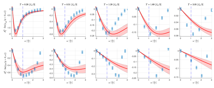
Figure 11: Transverse (top) and longitudinal (bottom) spin-spin correlation functions for a dimerized chain as a function of the frequency $\omega$ for a fixed wave vector $q=\pi$ and $\breve{q}=0$, respectively (see Eq. (14)). The field theory expression (13) in red is directly compared with the numerical T-DMRG calculation of the correlation (blue). The numerics are obtained from the Fourier transform of the output simulation without Gaussian filter (Sec. IV.1.4). We have taken $A_{x}^{\mathcal{D}}\simeq 0.1469$, $A_{z}^{\mathcal{D}}\simeq 0.082$, and $K^{\mathcal{D}}\simeq 0.754$. The shadow region corresponds to the maximum and minimum of all TLL parameters moving by $\pm 10\%$.

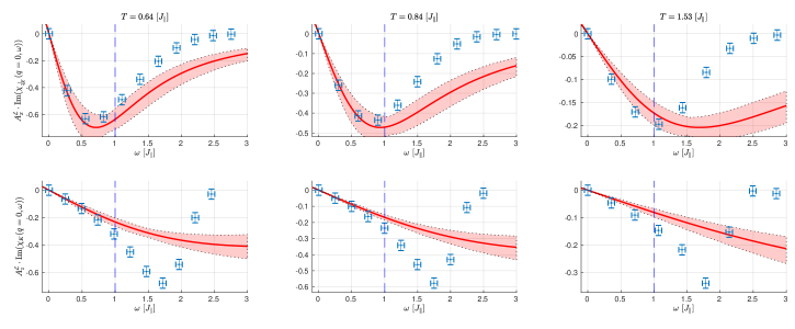
Figure 12: Transverse (top) and longitudinal (bottom) spin-spin correlation functions for a two-leg ladder as a function of the frequency $\omega$ for a fixed wave vector $q=\pi$ and $\breve{q}=0$, respectively (see Eq. (14)). The field theory expression (13) in red is directly compared with the numerical T-DMRG calculation of the correlation (blue). The numerics are obtained from the Fourier transform of the output simulation without Gaussian filter (Sec. IV.1.4). We have taken $A_{x}^{\mathcal{L}}\simeq 0.166$, $A_{z}^{\mathcal{L}}\simeq 0.078$, and $K^{\mathcal{L}}\simeq 0.85$. The shadow region corresponds to the maximum and minimum of all TLL parameters moving by $\pm 10\%$.

V.3 Bosonization and T-DMRG comparison

Since we have now fixed all the non-universal TLL parameters and amplitudes from Table 3, we can use the field theory expression (13) to obtain the correlation functions at finite temperature without any adjustable parameter. For the comparison between the direct numerical calculation of the correlations and the field theory, we consider the correlations at $q=\pi$ which are directly related to (16) and (13) by

$$\begin{split}A_{x}\operatorname{Im}\left(\chi_{\frac{1}{4K}}(\breve{q}=0,\omega)\right)&=\frac{1-e^{-\beta\omega}}{-2}\left\langle\mathds{S}^{x}(q=\pi,\omega)\mathds{S}^{x}\right\rangle\\ A_{z}\operatorname{Im}\left(\chi_{K}(\breve{q}=0,\omega)\right)&=\frac{1-e^{-\beta\omega}}{-2}\left\langle\delta\mathds{S}^{z}(q=\pi,\omega)\delta\mathds{S}^{z}\right\rangle\end{split}$$ (14)

The short-distance cutoff $\alpha$ can be taken as equal to $1$ inside the retarded susceptibility since it is reabsorbed in the non-universal amplitudes $A_{x}=\left(\frac{\alpha^{\frac{1}{2K}-1}}{4\pi a^{\frac{1}{2K}-1}}\right)$ and $A_{z}=\left(\frac{\alpha^{2K-2}}{a^{2K-2}2\pi^{2}}\right)$ according to definition (V.1), where $a$ is the lattice spacing unit cell.

Let us first compare the field theory prediction with the numerical calculations of the correlations for the anisotropic spin-$1/2$ chain. The result is shown in Fig. 10.

As can be seen from the slices 10, 11, and 12 the agreement is excellent both for the longitudinal and the transverse correlations, for temperatures up to $T\lesssim 0.5J$ for all frequencies up to $\omega\lesssim J$ at which one would expect in any case the field theory description to cease to be valid, irrespectively of the thermal effects. Note that the frequency regime for which the field theory is valid is much broader than what was the case for the NMR relaxation time Coira et al. (2016). This is probably due to the fact that here we focus on a specific value of $q$ (slice) for which massless modes down to zero energy exist, rather than perform a summation over all $q$ modes. It also confirms that for a quite broad range of temperatures and frequencies, the conformal modification of the zero-temperature correlations correctly gives the finite temperature behavior. At larger temperatures $T>0.64J$ and above, deviations start to appear, even if the low-energy part of the spectrum remains remarkably robust even at quite high temperatures. Note in particular the axis intensities in Fig. 10 that clearly show how well equation (13) predicts the low spectrum behavior.

Quite remarkably, a similar excellent agreement is found for dimer and ladder systems as, respectively, shown in Fig. 11 and Fig. 12. The range of temperatures and frequencies for which the low-energy effective theory works remarkably well is again quite broad. Both ladders and dimers also show an excellent agreement with the field theory prediction for frequencies up to the natural cutoff of the model, $J_{\parallel}$ for the two-leg ladder, or $J_{w}/2$ for the dimer system. For the ladder, although we can only reach the relatively high temperatures of more than half $J_{\parallel}$, the field theory remains quite excellent up to frequencies of order $\omega\lesssim J_{\parallel}$.

The extension of the TLL theory to finite temperature gives an excellent quantitative description of the correlations up to temperatures and energies close to the bandwidth of the problem. This very robust behavior of the field theory description, in a broad range of frequencies and temperatures, up to – and sometimes even beyond – the natural cutoff of the theory is of course directly relevant in the way that we can trust the application of such theories for treating more complex realizations (such as, e.g., coupled systems). This is of course especially important to tackle the physics of compounds with low enough magnetic exchanges, such that they can be manipulated by realistic magnetic fields. The drawback of such compounds is of course that the natural scale of energies (e.g., in a INS experiment) or temperatures that one can reach is getting closer to the magnetic exchange.

VI Conclusion

In this paper, we computed using a T-DMRG technique the dynamical structure factor of a two-leg spin-$1/2$ ladder system, as a function of the energy, momentum, and temperature. We use an optimal scheme for the implementation of the time evolution in order to be able to reach the necessary resolution for the two-leg ladder system. We focus on the intermediate magnetic field regime for which the magnetization per rung or per dimer is half of the saturation value. There the system has massless excitation and a low-energy part that can be mapped onto a Tomonaga-Luttinger liquid.

The results are indicated in Fig. 3 and Fig. 4. We compare these spectra with those of dimerized systems and of an anisotropic $\Delta=\frac{1}{2}$ XXZ chain, to which the low-energy part of the previous systems can be mapped. We examine in particular the evolution of the intermediate energy part of the spectrum getting thermally populated by the triplet $\left|t^{0}\right\rangle$. For the low-temperature part we examine the spin-chain mapping and compare the finite temperature correlations with the conformal modification of the TLL field theory. We show that there is an excellent agreement between the numerics and the field theory for energies and temperatures that extend up to values corresponding to the spin exchange of the weak-coupling energy scale ($J_{\parallel}$ for ladders and $J_{w}/2$ for dimers).

Our paper shows clearly the direct possibility to use with an excellent accuracy the field theory description to study more complex systems of ladders such as weakly three-dimensional coupled ladders even if the temperature or the interladder coupling reaches reasonably strong values. It also shows that for systems as complex as the ladders we have an essentially exact description even at finite temperatures from the numerics and similar features can be found in related models (that we have already analyzed in that way), namely, spin chains and dimerized systems.

Our calculation can potentially be directly comparable to measurements done with neutron scattering on two-leg ladder systems. Compounds such as (C₅H₁₂N)₂CuBr₄ (BPCB)Rüegg et al. (2008), (C₇H₁₀N)₂CuBr₄ (DIMPY)Schmidiger et al. (2013b), and (C₅H₁₂N)₂CuCl₄ (BPCC)Ward et al. (2017) are of course prime candidates for such study. Very successful comparisons of the broad features of the neutrons have already been done with the zero-temperature numerics and no high temperature as the one we have studied yet exists in the literature in the gapless regime. We hope that the present paper will stimulate experimentalists to perform these experiments, either in BPCB or in similar compounds at larger temperature $J_{\parallel}\lesssim T\lesssim J_{\perp}$, in particular to probe the $\left|t^{0}\right\rangle$ incoherent dispersion. For BPCB Bouillot et al. (2011), the couplings are, respectively, $J_{\parallel}\simeq 3.55~{}\text{K}$ and $J_{\perp}\simeq 12.6~{}\text{K}$ and the $\left|t^{0}\right\rangle$ mode is situated around the $J_{\perp}$ energy scale (see Figs. 3 and 4) and therefore located at a neutron energy of approximately $1~{}\text{meV}$. One could thus expect to see the change of behavior for the $\left|t^{0}\right\rangle$ mode, as described by Figs. 8 and 9, when going from $T=200~{}\text{mK}$ to $T=10~{}\text{K}$.

Our results open the door to a finer study of the temperature effects, or the study via numerics of the vicinity of quantum critical points in ladders for which such temperature effects are crucial to take into account.

Appendix A Convergence and precision

Note first that we use the Suzuki-Trotter decomposition in the normalized units of the biggest energy scale to be consistent with the diverse numerical precision and matrix conditioning.

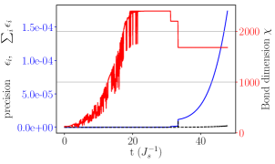
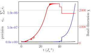
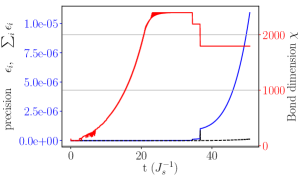
Figure 13: Example of how the precision – truncated weight $\epsilon_{i}$ (dashed black line), sum of all discarded weight $\sum_{i}\epsilon_{i}$ (solid blue line) and bond dimension $\chi$ (red line) – grows with the time for three different observables $e^{+iHt}\frac{e^{-\tilde{\beta}H}S^{\alpha}}{\sqrt{Z_{2\tilde{\beta}}}}e^{-iHt}$ in the ladder case at low temperature $\beta=2\tilde{\beta}=20.0~{}J_{s}^{-1}$. From top to bottom, we have $\alpha$ equal to “$+$”, “$-$” and “$z$”. The bond dimension truncation grows first until reaching $2400$. The computation starting to be too heavy, we reduce it to $2200$. Then after a computational time of the order of a few days we reduced it again to $1700$ to reach reasonable computational times.

As a rule of thumb, we set the maximal bond dimension for the problem ($\chi_{\mathcal{L}}=620$, $\chi_{\mathcal{D}}=2400$ ). Of course, it requires much less computational ressources to run the less consuming observables ($\frac{e^{-\beta H}}{Z}S^{-}$ and $\frac{e^{-\beta H}}{Z}S^{z}$, see Fig. 13) at smaller bond dimension $\chi$. However, the artificial oscillation would start at different precision scales which we try to avoid. We always start with some maximal value $\chi$ and then, if needed, reduce the bond dimension to more quickly reach the final resolution of the problem. This gives full accuracy for the initial short time evolution which reduces the possibility of cumulative errors.

We present in Fig. 13 a plot of the bond dimension with the truncated weight $\epsilon_{i}$ (one step) of the Suzuki-Trotter process and the sum of all discarded weights $\sum_{i}\epsilon_{i}$ (integration) for three observables.

The typically used measure of errors in the simulation, namely, the $\epsilon_{i}$, is shown as the dashed black curve. In this paper we, however, use the sum of all the discarded weights as the relevant error $\sum_{i}\epsilon_{i}$. We believe that this more stringent criterion helps to obtain results which are more accurate and reproducible.

Appendix B Lehmann representation and the detailed balance

The Lehmann representation consists of computing the averages using the exact eigenenergies $E_{n}$ and eigenvectors $|n\rangle$ of the Hamiltonian:

$$\left\langle A(t)B\right\rangle=\frac{1}{Z}\sum_{n,m}e^{-\beta E_{n}}e^{i(E_{n}-E_{m})t}\left\langle n\right|A\left|m\right\rangle\left\langle m\right|B\left|n\right\rangle$$

It follows that the imaginary part of the susceptibility has the following symmetries:

$$\operatorname{Im}(\chi^{\alpha\gamma}_{\text{ret}}(q,\omega))=-\operatorname{Im}(\chi^{\gamma\alpha}_{\text{ret}}(-q,-\omega))$$ (15)

due to

$${\scriptstyle\frac{-\pi}{Z}\sum_{n,m}(e^{-\beta E_{n}}-e^{-\beta E_{m}})\left\langle n\right|S^{\alpha}_{\frac{q}{2}}\left|m\right\rangle\left\langle m\right|S^{\gamma}_{-\frac{q}{2}}\left|n\right\rangle\delta(\omega+E_{n}-E_{m})=}$$

$${\scriptstyle\frac{-\pi}{Z}\sum_{n,m}(e^{-\beta E_{m}}-e^{-\beta E_{n}})\left\langle n\right|S^{\gamma}_{-\frac{q}{2}}\left|m\right\rangle\left\langle m\right|S^{\alpha}_{\frac{q}{2}}\left|n\right\rangle\delta(-\omega+E_{n}-E_{m})}$$

The dynamical structure factor is related to the imaginary part of the susceptibility

$$S^{\alpha\gamma}(q,\omega)=\frac{-2}{1-e^{-\beta\omega}}\operatorname{Im}(\chi^{\alpha\gamma}_{\text{ret}}(q,\omega))$$ (16)

due to

$${\scriptstyle\frac{-\pi}{Z}\sum_{n,m}(e^{-\beta E_{n}}-e^{-\beta E_{m}})\left\langle n\right|S^{\alpha}\left|m\right\rangle\left\langle m\right|S^{\gamma}\left|n\right\rangle\delta(\omega+E_{n}-E_{m})}=$$

$${\scriptstyle\frac{(1-e^{-\beta\omega})}{(-2)}\frac{(2\pi)}{Z}\sum_{n,m}e^{-\beta E_{n}}\left\langle n\right|S^{\alpha}\left|m\right\rangle\left\langle m\right|S^{\gamma}\left|n\right\rangle\delta(\omega+E_{n}-E_{m})}$$

Thus the detailed balance equation follows from the two equations (15) and (16)

$$S^{\alpha\gamma}(q,\omega)=e^{-\beta\omega}S^{\gamma\alpha}(-q,-\omega)$$ (17)

Appendix C Symmetries in ladders and dimers

For the ladder, the rung and leg inversion symmetries for the middle cell rung $\ell_{0}=\frac{N+1}{2}$ of a ladder with an odd number of rungs $N$ lead to

$$\left\langle S^{\alpha}_{\eta_{1},\ell}(t)S^{\gamma}_{\eta_{2},\ell_{0}}\right\rangle =\left\langle S^{\alpha}_{\eta_{2},-\ell}(t)S^{\gamma}_{\eta_{1},\ell_{0}}\right\rangle=$$

$$\left\langle S^{\alpha}_{\eta_{2},\ell}(t)S^{\gamma}_{\eta_{1},\ell_{0}}\right\rangle =\left\langle S^{\alpha}_{\eta_{1},-\ell}(t)S^{\gamma}_{\eta_{2},\ell_{0}}\right\rangle$$

with $\eta_{1},\eta_{2}\in\{1,2\}$. All correlations are space symmetric in the $\ell$ coordinate and we have equivalence between top-top and bottom-bottom correlations as well as bottom-top and top-bottom correlations. This makes the decomposition of the correlation in the $q_{\perp}\in\{0,\pi\}$ sectors appropriate.

For the dimer, there is only one rung or leg symmetry. For the middle rung cell $\ell_{0}=\frac{N+1}{2}$ and for an odd number of rungs, we have

$$\left\langle S^{\alpha}_{1,\ell}(t)S^{\gamma}_{1,\ell_{0}}\right\rangle =\left\langle S^{\alpha}_{2,-\ell}(t)S^{\gamma}_{2,\ell_{0}}\right\rangle\neq$$

$$\left\langle S^{\alpha}_{2,\ell}(t)S^{\gamma}_{2,\ell_{0}}\right\rangle =\left\langle S^{\alpha}_{1,-\ell}(t)S^{\gamma}_{1,\ell_{0}}\right\rangle$$

The left-left and right-right correlations have the same number of couplings in both $\ell$ directions with reversed order (strong$+$weak vs weak$+$strong). They are pretty similar up to boundary effects.

The left-right and right-left correlations

$$\left\langle S^{\alpha}_{1,\ell}(t)S^{\gamma}_{2,\ell_{0}}\right\rangle =\left\langle S^{\alpha}_{2,-\ell}(t)S^{\gamma}_{1,\ell_{0}}\right\rangle\neq$$

$$\left\langle S^{\alpha}_{2,\ell}(t)S^{\gamma}_{1,\ell_{0}}\right\rangle =\left\langle S^{\alpha}_{1,-\ell}(t)S^{\gamma}_{2,\ell_{0}}\right\rangle$$

are, however, very sensitive to the dimer geometry. For the first site correlations $\ell-\ell_{0}\in\{-1,+1\}$, one crosses different amounts of coupling in each direction (weak vs strong$+$weak). This asymmetry makes those correlations very sensitive to the dimerization structure even in the infinite-size limit. For those reasons, the $q_{\perp}\in\{0,\pi\}$ is not a valid quantum number for the dimer even though there exist many similarities with the ladder.

Appendix D Dimer spectrum along the chain direction

The main text presents the results of the dimer (see Fig. 5) using the two-leg ladder representation (as shown in Fig. 1). For completeness and more easy comparison with Ref. Coira et al., 2018 we also show in Fig. 14 the results in the chain geometry.

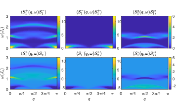
Figure 14: Correlations along the chain of the weakly coupled dimerized chain at $T=0.05~{}J_{s}$ with $J_{w}=0.39~{}J_{s}$ and $J_{s}=1$ for magnetic field corresponding to $m_{\mathcal{D}}\simeq 0.25$ (compare with Fig. 5). Note that, due to the geometry, the unit cells are now two sites periodic and the reciprocal space is $\pi$ periodic.

The figure shows how the left-left cell $\left\langle S^{\alpha}_{1}(q,\omega)S^{\gamma}_{1}\right\rangle$ and left-right cell $\left\langle S^{\alpha}_{1}(q,\omega)S^{\gamma}_{2}\right\rangle$ disperse.

References

- Bloch et al. (2008) I. Bloch, J. Dalibard, and W. Zwerger, Reviews of Modern Physics 80, 885 (2008).
- Cazalilla et al. (2011) M. A. Cazalilla, R. Citro, T. Giamarchi, E. Orignac, and M. Rigol, Reviews of Modern Physics 83, 1405 (2011).
- Auerbach (1994) A. Auerbach, Interacting Electrons and Quantum Magnetism, Graduate Texts in Contemporary Physics (Springer-Verlag, New York, 1994).
- Giamarchi (2003) T. Giamarchi, Quantum Physics in One Dimension, International Series of Monographs on Physics (Oxford University Press, Oxford, 2003).
- Dagotto and Rice (1996) E. Dagotto and T. M. Rice, Science 271, 618 (1996).
- Furrer et al. (2009) A. Furrer, J. Mesot, and T. Strässle, Neutron Scattering in Condensed Matter Physics (WORLD SCIENTIFIC, 2009) https://www.worldscientific.com/doi/pdf/10.1142/4870 .
- Berthier et al. (2017) C. Berthier, M. Horvatić, M.-H. Julien, H. Mayaffre, and S. Krämer, Comptes Rendus Physique 2016 Prizes of the French Academy of Sciences /Prix 2016 de l’Académie des sciences, 18, 331 (2017).
- Caux and Calabrese (2006) J.-S. Caux and P. Calabrese, Physical Review A 74, 031605 (2006).
- Thielemann et al. (2009a) B. Thielemann, C. Rüegg, H. M. Rønnow, A. M. Läuchli, J.-S. Caux, B. Normand, D. Biner, K. W. Krämer, H.-U. Güdel, J. Stahn, K. Habicht, K. Kiefer, M. Boehm, D. F. McMorrow, and J. Mesot, Physical Review Letters 102, 107204 (2009a).
- Thielemann et al. (2009b) B. Thielemann, C. Rüegg, K. Kiefer, H. M. Rønnow, B. Normand, P. Bouillot, C. Kollath, E. Orignac, R. Citro, T. Giamarchi, A. M. Läuchli, D. Biner, K. W. Krämer, F. Wolff-Fabris, V. S. Zapf, M. Jaime, J. Stahn, N. B. Christensen, B. Grenier, D. F. McMorrow, and J. Mesot, Physical Review B 79, 020408 (2009b).
- White (1992) S. R. White, Phys. Rev. Lett. 69, 2863 (1992).
- White (1993) S. R. White, Phys. Rev. B 48, 10345 (1993).
- Vidal (2003) G. Vidal, Phys. Rev. Lett. 91, 147902 (2003).
- Daley et al. (2004) A. J. Daley, C. Kollath, U. Schollwöck, and G. Vidal, Journal of Statistical Mechanics: Theory and Experiment 2004, P04005 (2004).
- Vidal (2004) G. Vidal, Phys. Rev. Lett. 93, 040502 (2004).
- White and Feiguin (2004) S. R. White and A. E. Feiguin, Phys. Rev. Lett. 93, 076401 (2004).
- Schollwöck (2011) U. Schollwöck, Annals of Physics 326, 96 (2011), january 2011 Special Issue.
- Bouillot et al. (2011) P. Bouillot, C. Kollath, A. M. Läuchli, M. Zvonarev, B. Thielemann, C. Rüegg, E. Orignac, R. Citro, M. Klanjšek, C. Berthier, M. Horvatić, and T. Giamarchi, Physical Review B 83, 054407 (2011).
- Schmidiger et al. (2013a) D. Schmidiger, S. Mühlbauer, A. Zheludev, P. Bouillot, T. Giamarchi, C. Kollath, G. Ehlers, and A. M. Tsvelik, Physical Review B 88, 094411 (2013a).
- Klanjšek et al. (2008) M. Klanjšek, H. Mayaffre, C. Berthier, M. Horvatić, B. Chiari, O. Piovesana, P. Bouillot, C. Kollath, E. Orignac, R. Citro, and T. Giamarchi, Physical Review Letters 101, 137207 (2008).
- Schmidiger et al. (2012) D. Schmidiger, P. Bouillot, S. Mühlbauer, S. Gvasaliya, C. Kollath, T. Giamarchi, and A. Zheludev, Physical Review Letters 108, 167201 (2012).
- Sachdev (1999) S. Sachdev, Quantum Phase Transitions (Cambridge University Press, 1999).
- Sachdev et al. (1994) S. Sachdev, T. Senthil, and R. Shankar, Physical Review B 50, 258 (1994).
- Verstraete et al. (2004) F. Verstraete, J. J. García-Ripoll, and J. I. Cirac, Phys. Rev. Lett. 93, 207204 (2004).
- Zwolak and Vidal (2004) M. Zwolak and G. Vidal, Phys. Rev. Lett. 93, 207205 (2004).
- Feiguin and White (2005) A. E. Feiguin and S. R. White, Phys. Rev. B 72, 220401 (2005).
- Barthel (2013) T. Barthel, New Journal of Physics 15, 073010 (2013).
- Barthel et al. (2009) T. Barthel, U. Schollwöck, and S. R. White, Physical Review B 79, 245101 (2009).
- Blosser et al. (2017) D. Blosser, N. Kestin, K. Y. Povarov, R. Bewley, E. Coira, T. Giamarchi, and A. Zheludev, Physical Review B 96, 134406 (2017).
- Becker et al. (2017) J. Becker, T. Köhler, A. C. Tiegel, S. R. Manmana, S. Wessel, and A. Honecker, Physical Review B 96, 060403 (2017).
- Lange et al. (2018) F. Lange, S. Ejima, and H. Fehske, Physical Review B 97, 060403 (2018).
- Klyushina et al. (2016) E. S. Klyushina, A. C. Tiegel, B. Fauseweh, A. T. M. N. Islam, J. T. Park, B. Klemke, A. Honecker, G. S. Uhrig, S. R. Manmana, and B. Lake, Physical Review B 93, 241109 (2016).
- Coira et al. (2016) E. Coira, P. Barmettler, T. Giamarchi, and C. Kollath, Physical Review B 94, 144408 (2016).
- Coira et al. (2018) E. Coira, P. Barmettler, T. Giamarchi, and C. Kollath, Physical Review B 98, 104435 (2018).
- Damle and Sachdev (1998) K. Damle and S. Sachdev, Physical Review B 57, 8307 (1998).
- Blosser et al. (2018) D. Blosser, V. K. Bhartiya, D. J. Voneshen, and A. Zheludev, Physical Review Letters 121, 247201 (2018).
- Ward et al. (2013) S. Ward, P. Bouillot, H. Ryll, K. Kiefer, K. W. Krämer, C. Rüegg, C. Kollath, and T. Giamarchi, Journal of Physics. Condensed Matter: An Institute of Physics Journal 25, 014004 (2013).
- Ward et al. (2017) S. Ward, M. Mena, P. Bouillot, C. Kollath, T. Giamarchi, K. P. Schmidt, B. Normand, K. W. Krämer, D. Biner, R. Bewley, T. Guidi, M. Boehm, D. F. McMorrow, and C. Rüegg, Physical Review Letters 118, 177202 (2017).
- Ryll et al. (2014) H. Ryll, K. Kiefer, C. Rüegg, S. Ward, K. W. Krämer, D. Biner, P. Bouillot, E. Coira, T. Giamarchi, and C. Kollath, Physical Review B 89, 144416 (2014).
- Tajiri et al. (2004) T. Tajiri, H. Deguchi, M. Mito, S. Takagi, H. Nojiri, T. Kawae, and K. Takeda, Journal of Magnetism and Magnetic Materials Proceedings of the International Conference on Magnetism (ICM 2003), 272-276, 1070 (2004).
- Suzuki (1991) M. Suzuki, Journal of Mathematical Physics 32, 400 (1991).
- McLachlan (1995) R. McLachlan, SIAM Journal on Scientific Computing 16, 151 (1995).
- Singh et al. (2011) S. Singh, R. N. C. Pfeifer, and G. Vidal, Physical Review B 83, 115125 (2011).
- Hubig et al. (2017) C. Hubig, I. P. McCulloch, and U. Schollwöck, Physical Review B 95, 035129 (2017).
- Eisert et al. (2010) J. Eisert, M. Cramer, and M. B. Plenio, Reviews of Modern Physics 82, 277 (2010).
- Tange (2015) O. Tange, “Gnu parallel 20150322 (’hellwig’),” (2015), GNU Parallel is a general parallelizer to run multiple serial command line programs in parallel without changing them.
- Schulz and Bourbonnais (1983) H. J. Schulz and C. Bourbonnais, Physical Review B 27, 5856 (1983).
- Chitra and Giamarchi (1997) R. Chitra and T. Giamarchi, Physical Review B 55, 5816 (1997).
- Giamarchi and Tsvelik (1999) T. Giamarchi and A. M. Tsvelik, Physical Review B 59, 11398 (1999).
- Hikihara and Furusaki (2001) T. Hikihara and A. Furusaki, Physical Review B 63, 134438 (2001).
- Dolfi et al. (2014) M. Dolfi, B. Bauer, S. Keller, A. Kosenkov, T. Ewart, A. Kantian, T. Giamarchi, and M. Troyer, Computer Physics Communications 185, 3430 (2014).
- Rüegg et al. (2008) C. Rüegg, K. Kiefer, B. Thielemann, D. F. McMorrow, V. Zapf, B. Normand, M. B. Zvonarev, P. Bouillot, C. Kollath, T. Giamarchi, S. Capponi, D. Poilblanc, D. Biner, and K. W. Krämer, Physical Review Letters 101, 247202 (2008).
- Schmidiger et al. (2013b) D. Schmidiger, P. Bouillot, T. Guidi, R. Bewley, C. Kollath, T. Giamarchi, and A. Zheludev, Physical Review Letters 111, 107202 (2013b).