Models of Collapsing and Expanding Cylindrical Source in $f(R,T)$ Theory

Abstract

We discuss the collapsing and expanding solutions of anisotropic charged cylinder in the context of $f(R,T)$ theory ($R$ represents the Ricci scalar and $T$ denotes the trace of energy-momentum tensor). For this purpose, we take an auxiliary solution of Einstein-Maxwell field equations and evaluate expansion scalar whose negative values lead to collapse and positive values give expansion. For both cases, the behavior of density, pressure, anisotropic parameter as well as mass is explored and the effects of charge as well as model parameter on these quantities are examined. The energy conditions are found to be satisfied for both solutions.

Keywords: $f(R,T)$ gravity; Self-gravitating objects; Electromagnetic theory.
PACS: 04.20.Jb; 04.40.Dg; 04.40.Nr; 04.50.Kd.

1 Introduction

Gravitational force is amenable for governing many astrophysical phenomena like formation of stars, keeping stars together in galaxies, gravitational collapse and restricting the heavenly bodies in their respective orbits. A star is in equilibrium state under the balance of pressure (directed outward) and gravity (directed inward). It undergoes collapse if gravity exceeds pressure and experiences expansion when pressure overcomes gravity. During the life, a star experiences both these phenomena. Oppenheimer and Snyder [1] are pioneers to study the gravitational collapse for dust matter. Misner and Sharp worked on the collapse of a star considering isotropic [2] as well as anisotropic fluid [3].

After that many researchers studied the process of collapse for different configurations. Stark and Piran [4] examined the gravitational waves emitted by the gravitational collapse of rotating relativistic polytropes. Herrera et al. [5] examined the dynamical instability of spherical symmetric collapsing fluid suffering heat dissipation and showed that dissipation increases the instability. Harada [6] investigated the final outcome of gravitational collapse of a sphere with perfect fluid distribution and discussed the limits when the singularity is naked or not. Joshi and Dwivedi [7] explored the final outcome of spherical symmetric dust collapse. Depending upon the initial pressure and density distribution, they discussed different new black hole solutions.

The $f(R)$ gravity is a direct generalization of general relativity (GR) obtained by replacing $R$ with $f(R)$ in the Einstein-Hilbert action. Many astrophysical and cosmological phenomena have been explored within the scenario of $f(R)$ theory. The contributions of $f(R)$ terms can lead different consequences on various phenomena. Sharif and Kausar [8] discussed the perfect fluid collapse in this theory and solved the equations assuming constant Ricci scalar. They showed that $f(R)$ terms play the role of anti gravitational force. Cembranos et al. [9] worked on spherical dust collapse and showed that the contribution of $f(R)$ terms slows down the collapsing process. Hence in general, it can be deduced that the inclusion of higher order curvature terms reduce the collapse rate. Also in GR, a gravitational wave has two polarization modes while in $f(R)$ theory it is shown that gravitational wave has two extra modes than GR [10].

Harko et al. [11] proposed a more generalized gravitational theory known as $f(R,T)$ gravity. The curvature-matter coupling produces a deviation from geodesic motion which may yield interesting results and help to explore dark side of the universe [12]. Shabani and Farhoudi [13] investigated cosmological viability of some $f(R,T)$ gravity models using solar system constraints. Moraes et al. [14] studied the equilibrium configurations of neutron and quark stars in this theory concluding that mass can cross observational limits. Noureen and Zubair [15] investigated the stability of anisotropic spherical star in the framework of $f(R,T)$ yielding some constraints on physical quantities. Carvalho et al. [16] analyzed white dwarfs using an Equation of state describing ionized atoms embedded in a relativistic Fermi gas of electrons in curvature-matter coupling scenario. They observed that white dwarfs have larger radius and mass in $f(R,T)$ gravity than those observed in GR and $f(R)$ theory.

Recent detection of gravitational waves has brought motivation to study the collapse phenomenon with the existence of gravitational waves in the exterior. It is well-known by Bhirkoff’s theorem that a spherical symmetric vacuum spacetime cannot have gravitational radiation. In this context, the next assumption is cylindrical system, because Einstein and Rosen found exact solution of the field equations which models the propagation of cylindrical gravitational waves. Sharif and Bhatti [17] discussed charged expansion-free cylindrical system and found that stability is controlled by charge, density and pressures. Yousaf et al. [18] discussed the stability of cylindrical stellar system through perturbation technique and found its dependence on the stiffness parameter, matter variables as well as $f(R,T)$ dark source terms. Sharif and Farooq investigated the dynamics of charged cylindrical collapse in $f(R)$ gravity with perfect [19] as well as bulk viscous dissipative fluid [20] and concluded that collapse rate slows down due to dark source terms.

Rosseland and Eddington [21] were the first who figured out the possibility that stars can have electric charge. After that the presence of electromagnetic field in self-gravitating systems is explored by many researchers. The effect of charge on spherical collapse [22] and on the stability of compact objects [23] have been investigated with the conclusion that charge halts the collapse as well as increases the stability regions. Bhatti and Yousaf [24] explored the effects of electromagnetic field on plane symmetric anisotropic dissipative fluid configuration in Palatini $f(R)$ gravity. They concluded that matter inhomogeneity is enhanced with charge while it is decreased due to modified gravity terms. Mansour et al. [25] analyzed the features of compact stars in the presence of weak electromagnetic field in $f(R)$ gravity.

Glass [26] studied the collapsing and expanding solutions for a non-static anisotropic spherical source within the scenario of GR. Abbas extended this work for plane symmetric configuration [27], charged spherical source [28] and for charged cylindrical geometry [29] in GR as well as for sphere in $f(R,T)$ gravity [30]. We discussed these solutions for charged spherical configuration in $f(R,T)$ theory [31]. In this paper, we investigate the effects of charge on the evolution of a non-static cylindrical source in $f(R,T)$ gravity. The paper is planned as follows. In the coming section, we discuss the outline of work done then in next one we formulate the Einstein-Maxwell equations for $f(R,T)=R+2\lambda T$ gravity model (where $\lambda$ is coupling constant also called model parameter) and discuss the cases of collapse and expansion. In the last section, we summarize our results.

2 Physical Goals

In this section, we first discuss physical goals of the research work presented in this paper and then elaborate the technique to achieve these objectives. Here, we would like to explore physical characteristics of a cylindrical star during the phases of collapse and expansion in the dark energy dominated era. When a star starts to loose the hydrostatic equilibrium, firstly, its outer layers expand and it becomes a red-giant. However, after some time, the star suffers a supernova explosion and experiences a collapse. In order to discuss the whole scenario in an expanding universe, we consider $f(R,T)$ theory of gravity as discussed in the introduction as an alternative to GR. Also, to extend our discussion, we observe the effects of electromagnetic field and consider a charged star. We aim to discuss the behavior of density, pressures, pressure anisotropy and mass of the star as well as check the energy conditions for the obtained solutions. We also investigate the effects of curvature-matter coupling and presence of charge on the collapse and expansion phases of the star’s life.

For this purpose, we generate collapsing and expanding solutions for our cylindrically symmetric model. We then analyze the physical parameters graphically such that the density and mass remain positive. Also, the obtained values of density and pressures must satisfy the energy conditions for the viability of the solution otherwise there is a possibility of existence of exotic fluid that is an unrealistic situation. The value of curvature-matter coupling constant is taken such that our model $f(R,T)=R+2\lambda T$ satisfies the viability conditions

$$f_{R}>0,\quad 1+\frac{f_{T}}{8\pi}>0\quad\text{and}\quad f_{RR}>0,$$

which yield the constraint $\lambda>-4\pi$ for the considered model. In the graphical analysis, free parameters appearing in the solution are fixed such that our solution is physically acceptable, i.e., mass as well as density are positive and energy conditions are satisfied. In order to examine the effects of electromagnetic field and curvature-matter coupling constant, we vary the values of the total charge and $\lambda$ in the plots and check the corresponding increase and decrease in the respective quantity.

3 Einstein-Maxwell Field Equations

The $f(R,T)$ gravity action with the contribution of electromagnetic field is defined as

$$S=\int d^{4}x\sqrt{-g}\left[\frac{1}{16\pi}f(R,T)+\mathcal{L}_{m}+\mathcal{L}_{e}\right].$$ (1)

The electromagnetic Lagrangian density $\mathcal{L}_{e}$ has the form $\mathcal{L}_{e}=mF_{\mu\nu}F^{\mu\nu},~{}m$ is an arbitrary constant, $F_{\mu\nu}=\phi_{\nu,\mu}-\phi_{\mu,\nu}$ represents the electromagnetic field tensor and $\phi_{\mu}$ represents the four potential. The field equations for the above action are

$$f_{R}R_{\mu\nu}-\frac{1}{2}g_{\mu\nu}f+(g_{\mu\nu}\Box-\nabla_{\mu}\nabla_{\nu})f_{R}=8\pi T_{\mu\nu}-f_{T}(T_{\mu\nu}+\Theta_{\mu\nu})+8\pi E_{\mu\nu},$$ (2)

where $f_{R}$ and $f_{T}$ denote the derivatives of $f(R,T)$ with respect to $R$ and $T$, respectively. The expression for $\Theta_{\mu\nu}$ is given by

$$\Theta_{\mu\nu}=g^{\gamma\alpha}\frac{\delta T_{\gamma\alpha}}{\delta g^{\mu\nu}},\quad T_{\mu\nu}=g_{\mu\nu}\mathcal{L}_{m}-\frac{\partial\mathcal{L}_{m}}{\partial g^{\mu\nu}},$$ (3)

and the electromagnetic energy-momentum tensor $E_{\mu\nu}$ is defined by

$$E_{\mu\nu}=\frac{1}{4\pi}\left(F_{\mu}^{~{}\alpha}F_{\nu\alpha}-\frac{1}{4}F^{\alpha\beta}F_{\alpha\beta}g_{\mu\nu}\right).$$ (4)

The non-static cylindrically symmetric spacetime is taken as

$$ds^{2}=-A^{2}(t,r)dt^{2}+B^{2}(t,r)dr^{2}+C^{2}(t,r)d\theta^{2}+dz^{2}.$$ (5)

The energy-momentum tensor for anisotropic fluid is given by

$$T_{\mu\nu}=(\rho+p_{r})V_{\mu}V_{\nu}+p_{r}g_{\mu\nu}-(p_{r}-p_{z})S_{\mu}S_{\nu}-(p_{r}-p_{\theta})K_{\mu}K_{\nu},$$ (6)

where $V_{\mu}$ denotes the four velocity, $S_{\mu}$, $K_{\mu}$ are unit four-vectors, $\rho$ stands for density, $p_{r}$, $p_{\theta}$, $p_{z}$ are the pressures in $r$, $\theta$ and $z$ directions, respectively. The four-vectors $V_{\mu}$, $S_{\mu}$ and $K_{\mu}$ have the expressions

$$V^{\mu}=(A^{-1},0,0,0),\quad K^{\mu}=(0,0,C^{-1},0),\quad S^{\mu}=(0,0,0,1),$$ (7)

which satisfy the following relations

$$V^{\mu}V_{\nu}=-1,~{}K^{\mu}K_{\nu}=S^{\mu}S_{\nu}=1,~{}S^{\mu}K_{\nu}=V^{\mu}K_{\nu}=V^{\mu}S_{\nu}=0.$$

The Maxwell equations are given by

$$F^{\mu\nu}_{~{}~{};\nu}=4\pi j^{\mu},$$ (8)

where $j^{\mu}$ represents the four current. In comoving frame, the four potential and four current are defined as

$$\phi_{\mu}=(\phi,0,0,0),\quad j_{\mu}=(\xi,0,0,0),$$ (9)

$\phi$, $\xi$ (both are functions of $t$ and $r$) represent electric scalar potential and charge density, respectively. The Maxwell equations for the metric (5) yield

$$\phi^{{}^{\prime\prime}}+\phi^{{}^{\prime}}\left(\frac{C^{\prime}}{C}-\frac{A^{\prime}}{A}-\frac{B^{\prime}}{B}\right) = 4\pi\xi AB^{2},$$ (10)

$$\dot{\phi}^{{}^{\prime}}+\phi^{{}^{\prime}}\left(\frac{\dot{C}}{C}-\frac{\dot{A}}{A}-\frac{\dot{B}}{B}\right) = 0.$$ (11)

Integration of Eq.(10) gives

$$\phi^{{}^{\prime}}=\frac{AB}{C}q,\quad q=4\pi\int_{0}^{r}\xi BCdr,$$ (12)

where $q$ is the total charge of the cylinder. We take $f(R,T)=R+2\lambda T$ proposed by Harko et al. [11] to explore the effects of curvature-matter coupling on collapsing and expanding solutions. This model has frequently been used in literature [32] which yields a power-law type scale factor and is able to discuss accelerated expansion of the universe. It corresponds to $\Lambda$CDM model with trace dependent cosmological constant or $\Lambda(T)$ gravity discussed by Poplawski [33]. The above mentioned expression of $f(R,T)$ and $\mathcal{L}_{m}=-\rho$ simplify the field equations as

$$G_{\mu\nu}=(8\pi+2\lambda)T_{\mu\nu}+2\lambda\rho g_{\mu\nu}+\lambda Tg_{\mu\nu}+8\pi E_{\mu\nu},$$ (13)

which produces the following set of equations

$$\frac{1}{B^{2}}\left[\frac{B^{\prime}C^{\prime}}{BC}-\frac{C^{\prime\prime}}{C}\right]+\frac{1}{A^{2}}\frac{\dot{B}\dot{C}}{BC}+\frac{A^{2}q^{2}}{C^{2}}=8\pi\rho-\lambda(-\rho+p_{r}+p_{\theta}+p_{z}),$$ (14)

$$\frac{\dot{C}^{\prime}}{C}-\frac{\dot{C}}{C}\frac{A^{\prime}}{A}-\frac{\dot{B}}{B}\frac{C^{\prime}}{C}=0,$$ (15)

$$\frac{1}{A^{2}}\left[\frac{\dot{A}C^{\prime}}{AC}-\frac{\ddot{C}}{C}\right]+\frac{1}{B^{2}}\frac{A^{\prime}C^{\prime}}{AC}+\frac{B^{2}q^{2}}{C^{2}}=8\pi p_{r}+\lambda(\rho+3p_{r}+p_{\theta}+p_{z}),$$ (16)

$$\frac{1}{A^{2}}\left[\frac{\dot{A}\dot{B}}{AB}-\frac{\ddot{B}}{B}\right]+\frac{1}{C^{2}}\left(\frac{\dot{C}}{B}\right)^{2}\left[\frac{A^{\prime\prime}}{A}-\frac{A^{\prime}B^{\prime}}{AB}\right]-\frac{q^{2}}{C^{2}}=8\pi p_{\theta}$$

$$+\lambda(\rho+p_{r}+3p_{\theta}+p_{z}),$$ (17)

$$\frac{1}{A^{2}}\left[-\frac{\ddot{B}}{B}-\frac{\ddot{C}}{C}-\frac{\dot{B}\dot{C}}{BC}+\frac{\dot{A}}{A}\left(\frac{\dot{B}}{B}+\frac{\dot{C}}{C}\right)\right]+\frac{1}{B^{2}}\left[\frac{A^{\prime\prime}}{A}+\frac{C^{\prime\prime}}{C}-\frac{A^{\prime}B^{\prime}}{AB}\right.$$

$$\left.-\frac{C^{\prime}}{C}\left(\frac{B^{\prime}}{B}+\frac{A^{\prime}}{A}\right)\right]-\frac{q^{2}}{C^{2}}=8\pi p_{z}+\lambda(\rho+p_{r}+p_{\theta}+3p_{z}),$$ (18)

where dot and prime represent differentiation with respect to $t$ and $r$, respectively.

A simultaneous solution of the field equations give the following explicit expressions of density and pressure components

$$\rho = \frac{1}{8(8\pi^{2}+6\pi\lambda+\lambda^{2})A^{3}B^{3}C^{2}}\left[q^{2}(8\pi+5\lambda)A^{5}B^{3}-2AB^{2}C(-2(2\pi\right.$$ (19)

$$+ \left.\lambda)\dot{B}\dot{C}+\lambda(C\ddot{B}+B\ddot{C}))+\lambda B^{2}C\dot{A}(2C\dot{B}+B(\dot{C}+2C^{\prime}))-\lambda A^{2}\right.$$

$$\times \left.(C^{2}+\dot{C}^{2})(A^{\prime}B^{\prime}-BA^{\prime\prime})+A^{3}(-2q^{2}\lambda B^{3}+q^{2}\lambda B^{5}+4(2\pi+\lambda)\right.$$

$$\times \left.CB^{\prime}C^{\prime}-4(2\pi+\lambda)BCC^{\prime\prime})\right],$$

$$p_{r} = \frac{1}{8(2\pi+\lambda)(4\pi+\lambda)A^{3}B^{3}C^{2}}\left[-q^{2}\lambda A^{5}B^{3}+q^{2}A^{3}B^{3}(2\lambda+(8\pi\right.$$ (20)

$$+ \left.3\lambda)B^{2})-2AB^{2}C(-\lambda C\ddot{B}+(4\pi+\lambda)B\ddot{C})+B^{2}C\dot{A}(-2\lambda C\dot{B}\right.$$

$$+ \left.B(-\lambda\dot{C}+2(8\pi+3\lambda)C^{\prime}))+A^{2}(4(2\pi+\lambda)BCA^{\prime}C^{\prime}+\lambda(C^{2}\right.$$

$$+ \left.\dot{C}^{2})(A^{\prime}B^{\prime}-BA^{\prime\prime}))\right],$$

$$p_{\theta} = \frac{1}{8(2\pi+\lambda)(4\pi+\lambda)A^{3}B^{3}q^{2}}\left[-q^{2}\lambda A^{5}B^{3}-q^{2}A^{3}B^{3}(8\pi+2\lambda\right.$$ (21)

$$+ \left.\lambda B^{2})-2AB^{2}C((4\pi+\lambda)C\ddot{B}-\lambda B\ddot{C})+B^{2}C\dot{A}(2(4\pi+\lambda)C\dot{B}\right.$$

$$- \left.\lambda B(\dot{C}+2C^{\prime}))+A^{2}(\lambda C^{2}-(8\pi+3\lambda)\dot{C}^{2})(A^{\prime}B^{\prime}-BA^{\prime\prime})\right],$$

$$p_{z} = \frac{-1}{8(2\pi+\lambda)(4\pi+\lambda)A^{3}B^{3}C^{2}}\left[q^{2}\lambda A^{5}B^{3}+2AB^{2}C(2(2\pi+\lambda)\dot{B}\dot{C}\right.$$ (22)

$$+ \left.(4\pi+\lambda)(C\ddot{B}+B\ddot{C}))-B^{2}C\dot{A}(2(4\pi+\lambda)C\dot{B}+B((8\pi+3\lambda)\right.$$

$$\times \left.\dot{C}-2\lambda C^{\prime}))+A^{2}(4(2\pi+\lambda)BCA^{\prime}C^{\prime}+(8\pi+3\lambda)C^{2}(A^{\prime}B^{\prime}\right.$$

$$- \left.BA^{\prime\prime})+\lambda\dot{C}^{2}(-A^{\prime}B^{\prime}+BA^{\prime\prime}))+A^{3}(2q^{2}(4\pi+\lambda)B^{3}+q^{2}\lambda B^{5}\right.$$

$$+ \left.4(2\pi+\lambda)CB^{\prime}C^{\prime}-4(2\pi+\lambda)BCC^{\prime\prime})\right].$$

The anisotropic parameter is defined as

$$\triangle=p_{r}-p_{\theta}.$$ (23)

To investigate the collapse and expansion of considered cylindrical source, the expansion scalar is evaluated as

$$\Theta=\frac{1}{A}\left(\frac{\dot{B}}{B}+\frac{\dot{C}}{C}\right),$$ (24)

and an auxiliary solution of Eq.(15) is

$$A=\frac{\dot{C}}{\alpha C^{\gamma}},\quad B=\alpha C^{\gamma},$$ (25)

where $\gamma$ and $\alpha>0$ are arbitrary constants. The above solution leads to

$$\Theta=\alpha(1+\gamma)C^{\gamma-1}.$$ (26)

The positive values of $\Theta$ provide expansion and its negative values correspond to collapse. The value of $\Theta$ depends on $\alpha,~{}\gamma$ and $C$ in which $\alpha$ and $C$ are always positive implying that we have collapse for $\gamma<-1$ and expansion for $\gamma>-1$. We explore these cases one by one in the following subsections.

3.1 Collapse for $\gamma<-1$

For collapsing solution, we find the unknown metric function $C$ in the solution (25) such that the collapse leads to the formation of trapped surfaces. The mass function for the cylindrically symmetric charged source is obtained as

$$m(t,r)=\frac{1}{8}\left[1-\left(\frac{C^{\prime}}{B}\right)^{2}+\left(\frac{\dot{C}}{A}\right)^{2}\right]+qC.$$ (27)

Equation (25) simplifies the mass expression as

$$m(t,r)=\frac{1}{8}\left(1+\alpha^{2}C^{2\gamma}-\frac{C^{\prime 2}}{\alpha^{2}C^{2\gamma}}\right)+qC.$$ (28)

For trapped surface formation $m=\frac{1}{8}+qC$ [29], which yields

$$C_{trap}=\left[\alpha^{2}(1-2\gamma)r+g(t)\right]^{\frac{1}{1-2\gamma}},$$ (29)

where $g(t)$ is an integration function and the collapsing solution becomes

$$A = \frac{1}{\alpha(1-2\gamma)}\dot{g}\left(\alpha^{2}(1-2\gamma)r+g(t)\right)^{\frac{\gamma}{1-2\gamma}},$$ (30)

$$B = \alpha\left(\alpha^{2}(1-2\gamma)r+g(t)\right)^{\frac{\gamma}{1-2\gamma}},$$ (31)

$$C_{trap} = \left(\alpha^{2}(1-2\gamma)r+g(t)\right)^{\frac{1}{1-2\gamma}}.$$ (32)

For the sake of simplicity, we consider $g(t)$ as a linear function of $t$, i.e., $g(t)=\frac{t}{\alpha^{2}}$ and obtain the following expressions of density and pressures

$$\rho = \frac{\left(\frac{t}{\alpha^{2}}+r(1-2\gamma)\alpha^{2}\right)^{\frac{2+4\gamma}{2\gamma-1}}}{8(1-2\gamma)^{2}(8\pi^{2}+6\pi\lambda+\lambda^{2})\alpha^{6})}\left[q^{2}(8\pi+5\lambda)\left(\frac{t}{\alpha^{2}}+r(1-2\gamma)\alpha^{2}\right)^{\frac{6\gamma}{1-2\gamma}}\right.$$ (33)

$$- \left.\frac{1}{(t+r(1-2\gamma)\alpha^{4})^{2}}\left(2(1-2\gamma)^{2}\gamma(-4\pi+(-1+3\gamma)\lambda)\alpha^{12}\right.\right.$$

$$\times \left.\left.\left(\frac{t}{\alpha^{2}}+r(1-2\gamma)\alpha^{2}\right)^{\frac{2+2\gamma}{1-2\gamma}}\right)+\frac{\gamma(-1+2\gamma)\lambda\alpha^{12}\left(\frac{t}{\alpha^{2}}+r(1-2\gamma)\alpha^{2}\right)^{\frac{2+2\gamma}{1-2\gamma}}}{(t+r(1-2\gamma)\alpha^{4})^{4}}\right.$$

$$\times \left.(1+t^{2}(1-2\gamma)^{2}-2rt(-1+2\gamma)^{3}\alpha^{4}+r^{2}(1-2\gamma)^{4}\alpha^{8})-\frac{1}{(t+r(1-2\gamma)\alpha^{4})^{2}}\right.$$

$$\times \left.\left((1-2\gamma)^{2}\gamma\lambda\alpha^{12}\left(\frac{t}{\alpha^{2}}+r(1-2\gamma)\alpha^{2}\right)^{\frac{2+2\gamma}{1-2\gamma}}(-1-2\alpha^{4}+\gamma(-2+4\alpha^{4}))\right)\right.$$

$$+ \left.(1-2\gamma)^{2}\alpha^{3}\left(\frac{t}{\alpha^{2}}+r(1-2\gamma)\alpha^{2}\right)^{\frac{\gamma}{1-2\gamma}}\left\{-2q^{2}\lambda\alpha^{3}\left(\frac{t}{\alpha^{2}}+r(1-2\gamma)\alpha^{2}\right)^{\frac{3\gamma}{1-2\gamma}}\right.\right.$$

$$+ \left.\left.q^{2}\lambda\alpha^{5}\left(\frac{t}{\alpha^{2}}+r(1-2\gamma)\alpha^{2}\right)^{\frac{5\gamma}{1-2\gamma}}+4\gamma(2\pi+\lambda)\alpha^{5}\left(\frac{t}{\alpha^{2}}+r(1-2\gamma)\alpha^{2}\right)^{\frac{5\gamma}{1-2\gamma}}\right.\right.$$

$$- \left.\left.\frac{1}{(t+r(1-2\gamma)\alpha^{4})^{2}}8\gamma(2\pi+\lambda)\alpha^{9}\left(\frac{t}{\alpha^{2}}+r(1-2\gamma)\alpha^{2}\right)^{\frac{2+\gamma}{1-2\gamma}}\right\}\right],$$

$$p_{r} = \frac{\left(\frac{t}{\alpha^{2}}+r(1-2\gamma)\alpha^{2}\right)^{\frac{2+4\gamma}{2\gamma-1}}}{8(1-2\gamma)^{2}(2\pi^{2}+\lambda)(4\pi^{2}+\lambda)\alpha^{6})}\left[-q^{2}\lambda\left(\frac{t}{\alpha^{2}}+r(1-2\gamma)\alpha^{2}\right)^{\frac{6\gamma}{1-2\gamma}}\right.$$ (34)

$$+ \left.\frac{1}{(t+r(1-2\gamma)\alpha^{4})^{2}}\left(2(1-2\gamma)^{2}\gamma(-8\pi+3(-1+\gamma)\lambda)\alpha^{12}\right.\right.$$

$$\times \left.\left.\left(\frac{t}{\alpha^{2}}+r(1-2\gamma)\alpha^{2}\right)^{\frac{2+2\gamma}{1-2\gamma}}\right)+(q-2q\gamma)^{2}\alpha^{6}\left(\frac{t}{\alpha^{2}}+r(1-2\gamma)\alpha^{2}\right)^{\frac{4\gamma}{1-2\gamma}}\right.$$

$$\times \left.(2\lambda+(8\pi+3\lambda)\alpha^{2}\left(\frac{t}{\alpha^{2}}+r(1-2\gamma)\alpha^{2}\right)^{\frac{2\gamma}{1-2\gamma}})-(-8\pi(-1+2\gamma)\right.$$

$$\times \left.(t+r(1-2\gamma)\alpha^{4})^{2}+\lambda(1+t^{2}(5-12\gamma+4\gamma^{2})-2rt(1-2\gamma)^{2}(-5+2\gamma)\alpha^{4}\right.$$

$$+ \left.r^{2}(-5+2\gamma)(-1+2\gamma)^{3}\alpha^{3}))((t+r(1-2\gamma)\alpha^{4})^{4}\gamma(-1+2\gamma)\alpha^{12}\right.$$

$$\times \left.\left(\frac{t}{\alpha^{2}}+r(1-2\gamma)\alpha^{2}\right)^{\frac{2+2\gamma}{1-2\gamma}})-\frac{1}{(t+r(1-2\gamma)\alpha^{4})^{2}}(1-2\gamma)^{2}\gamma\alpha^{12}\right.$$

$$\times \left.\left(\frac{t}{\alpha^{2}}+r(1-2\gamma)\alpha^{2}\right)^{\frac{2+2\gamma}{1-2\gamma}}(16\pi(-1+2\gamma)\alpha^{4}\right.$$

$$+ \left.\lambda(1-6\alpha^{4}+2\gamma(1+6\alpha^{4})))\right],$$

$$p_{\theta} = \frac{\left(\frac{t}{\alpha^{2}}+r(1-2\gamma)\alpha^{2}\right)^{\frac{2+4\gamma}{-1+2\gamma}}}{8(1-2\gamma)^{2}(2\pi+\lambda)(4\pi+\lambda)\alpha^{6}}\left[-q^{2}\lambda\left(\frac{t}{\alpha^{2}}+r(1-2\gamma)\alpha^{2}\right)^{\frac{6\gamma}{1-2\gamma}}\right.$$ (35)

$$- \left.\frac{2(1-2\gamma)^{2}\gamma(4\pi(-1+3\gamma)+3(-1+\gamma)\lambda)\alpha^{12}\left(\frac{t}{\alpha^{2}}+r(1-2\gamma)\alpha^{2}\right)^{\frac{2+2\gamma}{1-2\gamma}}}{(t+r(1-2\gamma)\alpha^{4})^{2}}\right.$$

$$+ \left.\frac{(1-2\gamma)^{2}\gamma\alpha^{12}\left(\frac{t}{\alpha^{2}}+r(1-2\gamma)\alpha^{2}\right)^{\frac{2+2\gamma}{1-2\gamma}}}{(t+r(1-2\gamma)\alpha^{4})^{2}}(8\pi\gamma+(-1+2\gamma)\lambda(1+2\alpha^{4}))\right.$$

$$+ \left.\frac{(1-2\gamma)^{3}\gamma\alpha^{12}\left(\frac{t}{\alpha^{2}}+r(1-2\gamma)\alpha^{2}\right)^{\frac{2+2\gamma}{1-2\gamma}}}{(t+r(1-2\gamma)\alpha^{4})^{2}}\left(\lambda-\frac{8\pi+3\lambda}{(1-2\gamma)^{2}(t+r(1-2\gamma)\alpha^{4})^{2}}\right.\right.$$

$$- \left.\left.q^{2}(1-2\gamma)^{2}\alpha^{6}\right)\left(\frac{t}{\alpha^{2}}+r(1-2\gamma)\alpha^{2}\right)^{\frac{4\gamma}{1-2\gamma}}\left(8\pi+\lambda\left(2+\alpha^{2}\right.\right.\right.$$

$$\times \left.\left.\left.\left(\frac{t}{\alpha^{2}}+r(1-2\gamma)\alpha^{2}\right)^{\frac{2\gamma}{1-2\gamma}}\right)\right)\right],$$

$$p_{z} = \frac{\alpha^{6}\left(\frac{t}{\alpha^{2}}+r(1-2\gamma)\alpha^{2}\right)^{\frac{2+2\gamma}{-1+2\gamma}}}{8(1-2\gamma)^{2}(2\pi+\lambda)(4\pi+\lambda)}\left[8\pi(1-2\gamma)^{2}\left(\frac{-2\gamma\left(\frac{t}{\alpha^{2}}+r(1-2\gamma)\alpha^{2}\right)^{\frac{2}{1-2\gamma}}}{(t+r(1-2\gamma)\alpha^{4})^{2}}\right.\right.$$ (36)

$$- \left.\left.\frac{q^{2}\left(\frac{t}{\alpha^{2}}+r(1-2\gamma)\alpha^{2}\right)^{\frac{2\gamma}{1-2\gamma}}}{\alpha^{6}}\right)+\lambda\left(\frac{-q^{2}\left(\frac{t}{\alpha^{2}}+r(1-2\gamma)\alpha^{2}\right)^{\frac{2\gamma}{1-2\gamma}}}{\alpha^{12}}\right.\right.$$

$$\times \left.\left.\left(2(1-2\gamma)^{2}\alpha^{6}+\left(\frac{t}{\alpha^{2}}+r(1-2\gamma)\alpha^{2}\right)^{\frac{2\gamma}{1-2\gamma}}+(1-2\gamma)^{2}\alpha^{6}\right.\right.\right.$$

$$\times \left.\left.\left.\left(\frac{t}{\alpha^{2}}+r(1-2\gamma)\alpha^{2}\right)^{\frac{2\gamma}{1-2\gamma}}\right)+(-1+(4rt(1-2\gamma)^{2}\alpha^{4}+2r^{2}(-1+2\gamma)^{3}\alpha^{8})\right.\right.$$

$$\times \left.\left.(-3+\gamma-\alpha^{4}+2\gamma\alpha^{4}+2t^{2}(3+\alpha^{4}+\gamma^{2}(2+4\alpha^{4})-\gamma(7+4\alpha^{4}))))\right.\right.$$

$$\times \left.\left.\left((t+r(1-2\gamma)\alpha^{4})^{4}\gamma(-1+2\gamma)\left(\frac{t}{\alpha^{2}}+r(1-2\gamma)\alpha^{2}\right)^{\frac{2}{1-2\gamma}}\right)^{-1}\right)\right].$$

For the solution (30)-(32), the anisotropic parameter and mass function become

$$\triangle = \frac{\alpha^{6}\left(\frac{t}{\alpha^{2}}+r(1-2\gamma)\alpha^{2}\right)^{\frac{2+2\gamma}{-1+2\gamma}}}{8(1-2\gamma)(4\pi+\lambda)}\left[-q^{2}(-1+\gamma)\alpha^{-6}\left(\frac{t}{\alpha^{2}}+r(1-2\gamma)\alpha^{2}\right)^{\frac{2\gamma}{1-2\gamma}}\right.$$ (37)

$$\times \left.\left(1+\alpha^{2}\left(\frac{t}{\alpha^{2}}+r(1-2\gamma)\alpha^{2}\right)^{\frac{2\gamma}{-1+2\gamma}}\right)+\left(1-4rt(1-2\gamma)^{2}\alpha^{4}(1-\alpha^{4}\right.\right.$$

$$- \left.\left.\gamma(-1+2\alpha^{4}))+2r^{2}(-1+2\gamma)^{3}\alpha^{8}(1-\alpha^{8}-\gamma(-1+2\alpha^{4}))\right.\right.$$

$$+ \left.\left.\frac{2t^{2}(-1+\alpha^{4}+\gamma(3-4\alpha^{4})+\gamma^{2}(-2+4\alpha^{4}))}{(t+r(1-2\gamma)\alpha^{4})^{4}\gamma\left(\frac{t}{\alpha^{2}}+r(1-2\gamma)\alpha^{2}\right)^{\frac{2}{-1+2\gamma}}}\right)\right],$$

$$m = \frac{1}{8}+q\left(\frac{t}{\alpha^{2}}+r(1-2\gamma)\alpha^{2}\right)^{\frac{1}{1-2\gamma}}.$$ (38)

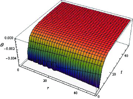
Figure 1: Plot of $\Theta$ versus $r$ and $t$ for $\gamma=-1.5$, $\alpha=0.1$.

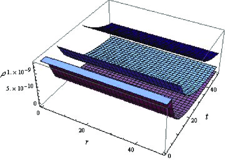
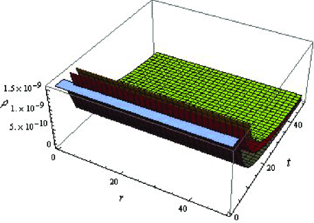
Figure 2: Plots of $\rho$ versus $r$ and $t$ for $\gamma=-1.5$, $\alpha=0.1$. The left graph is for $q=0$ (pink), $q=0.00005$ (blue), $q=0.0001$ (purple) with $\lambda=-0.1$ and the right graph is for $\lambda=-0.1$ (brown), $\lambda=-0.2$ (red), $\lambda=-0.3$ (yellow) with $q=0.0001$.

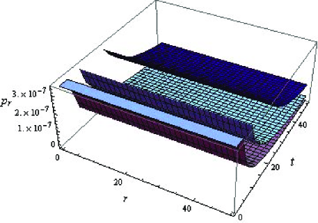
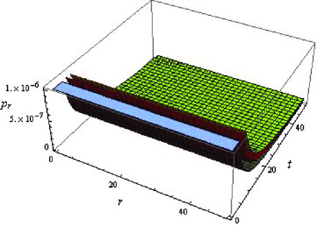
Figure 3: Plots of $p_{r}$ versus $r$ and $t$ for $\gamma=-1.5$, $\alpha=0.1$. The left graph is for $q=0$ (pink), $q=0.01$ (blue), $q=0.02$ (purple) with $\lambda=-0.1$ while the right graph is for $\lambda=-0.1$ (brown), $\lambda=-0.2$ (red), $\lambda=-0.3$ (yellow) with $q=0.01$.

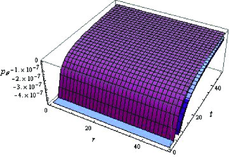
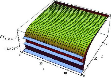
Figure 4: Plots of $p_{\theta}$ versus $r$ and $t$ for $\gamma=-1.5$, $\alpha=0.1$. The left graph is for $q=0$ (pink), $q=0.005$ (blue), $q=0.01$ (purple) with $\lambda=-0.1$ and the right graph is for $\lambda=-0.1$ (brown), $\lambda=-0.15$ (red), $\lambda=-0.2$ (yellow) with $q=0.01$.

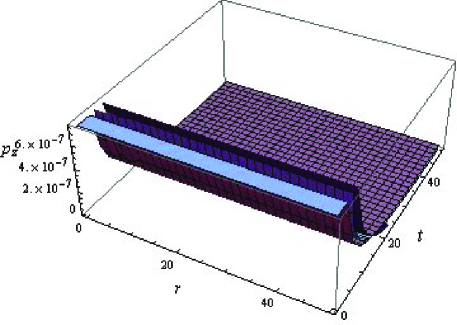
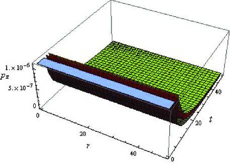
Figure 5: Plots of $p_{z}$ versus $r$ and $t$ for $\gamma=-1.5$, $\alpha=0.1$. The left graph is for $q=0$ (pink), $q=0.01$ (blue), $q=0.02$ (purple) with $\lambda=-0.1$ and the right graph is for $\lambda=-0.1$ (brown), $\lambda=-0.2$ (red), $\lambda=-0.3$ (yellow) with $q=0.01$.

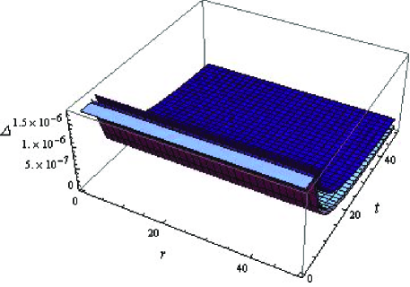
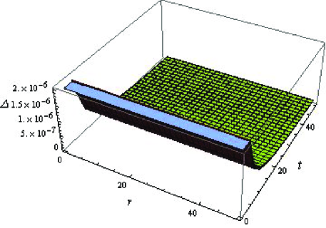
Figure 6: Plots of $\triangle$ versus $r$ and $t$ for $\gamma=-1.5$, $\alpha=0.1$. The left graph is for $q=0$ (pink), $q=0.01$ (blue), $q=0.02$ (purple) with $\lambda=-0.1$ and the right graph is for $\lambda=-0.1$ (brown), $\lambda=-0.2$ (red), $\lambda=-0.3$ (yellow) with $q=0.01$.

For the collapsing case, the graphical representation of different parameters is given in Figures 1-7. We observe that the quantities are changing with respect to temporal coordinate while no change is observed with respect to radial coordinate. The change in different quantities with respect to time is given in Table 1 and the effects of charge as well as model parameter $\lambda$ are summarized in Table 2.

Table 1: Change in parameters with respect to $t$ for the collapse solution

Parameter	$\rho$	$p_{r}$	$p_{\theta}$	$p_{z}$	$\triangle$	$m$
As $t$ increases	decreases	decreases	increases	decreases	decreases	increases

Table 2: Effects of $q$ and $\lambda$ for the collapse solution

Parameter	$\rho$	$p_{r}$	$p_{\theta}$	$p_{z}$	$\triangle$	$m$
As $q$ increases	increases	increases	decreases	decreases	increases	increases
As $\lambda$ decreases	increases	increases	increases	increases	increases	no change

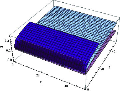
Figure 7: Plot of $m$ versus $r$ and $t$ for $\gamma=-1.5$, $\alpha=0.1$, $q=0$ (pink), $q=0.01$ (blue), $q=0.02$ (purple).

To observe physical viability of our solution, we plot the null (NEC), weak (WEC), strong (SEC) and dominant (DEC) energy conditions for the curvature-matter coupled gravity [35]

• NEC: $\rho+p_{r}-\mathcal{A}\geq 0,~{}\rho+p_{\theta}-\mathcal{A}\geq 0,~{}\rho+p_{z}-\mathcal{A}\geq 0$,

• WEC: $\rho-\mathcal{A}\geq 0,~{}\rho+p_{r}-\mathcal{A}\geq 0,~{}\rho+p_{\theta}-\mathcal{A}\geq 0,~{}\rho+p_{z}-\mathcal{A}\geq 0,$

• SEC: $\rho+p_{r}+p_{\theta}+p_{z}-\mathcal{A}\geq 0$.

• DEC: $\rho-p_{r}-\mathcal{A}\geq 0,~{}\rho+p_{\theta}-\mathcal{A}\geq 0,~{}\rho-p_{z}-\mathcal{A}\geq 0$,

The term $\mathcal{A}=(V^{\beta}V^{\alpha}_{;\beta})_{;\alpha}$ is due to non-geodesic motion of massive particles. We evaluate $\mathcal{A}$ as

$$\mathcal{A}=\frac{1}{B^{2}}\left[\frac{A^{\prime\prime}}{A}+\frac{A^{\prime}}{A}\left(-\frac{B^{\prime}}{B}+\frac{C^{\prime}}{C}+\frac{A^{\prime}}{A}\right)\right]+\frac{\dot{A}^{2}}{A^{4}}.$$ (39)

For the collapse solution, we have

$$\mathcal{A}=\frac{4\gamma^{2}\alpha^{6}\left(\frac{t}{\alpha^{2}}+r(1-2\gamma)\alpha^{2}\right)^{\frac{2\gamma}{-1+2\gamma}}}{(t+r(1-2\gamma)\alpha^{4})^{2}}.$$ (40)

All the energy conditions defined above are plotted in Figures 8-11, the repeated expressions are shown only once. From these plots, it can be easily seen that all the energy conditions are satisfied for the considered values of free parameters of the collapse solution.

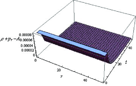
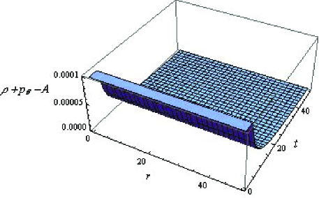
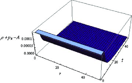
Figure 8: Plots for NEC for $\gamma=-1.5$, $\alpha=0.1$, $q=0.01$ and $\lambda=-0.1$.

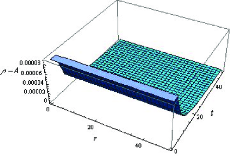
Figure 9: Plot for WEC for $\gamma=-1.5$, $\alpha=0.1$, $q=0.01$ and $\lambda=-0.1$.

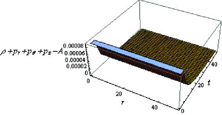
Figure 10: Plot for SEC for $\gamma=-1.5$, $\alpha=0.1$, $q=0.01$ and $\lambda=-0.1$.

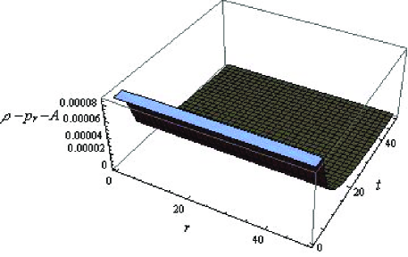
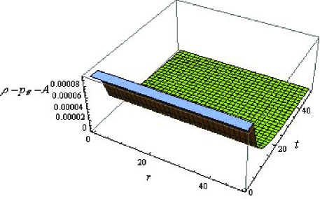
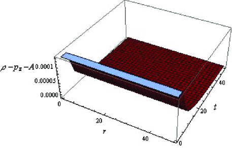
Figure 11: Plots for DEC for $\gamma=-1.5$, $\alpha=0.1$, $q=0.01$ and $\lambda=-0.1$.

3.2 Expansion for $\gamma>-1$

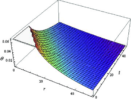
Figure 12: Plot of $\Theta$ versus $r$ and $t$ for $\gamma=0.0001$, $\alpha=1$.

In this case, we require an expression of the metric coefficient $C$ for expanding solution. For convenience, We assume it a linear combination of $r$ and $t$ such that the expansion scalar remains positive for the resulting solution as shown in Figure 12. Thus the expanding solution is given by

$$A=\frac{1}{\alpha(r+t)^{\gamma}},\quad B=\alpha(r+t)^{\gamma},\quad C=r+t.$$ (41)

Consequently, the expressions of $\rho$, $p_{r}$, $p_{\theta}$ and $p_{z}$ take the form

$$\rho = \frac{(r+t)^{-2(2+\gamma)}}{8(8\pi^{2}+6\pi\lambda+\lambda^{2})\alpha^{2}}\left[8\pi(r+t)^{2}(q^{2}+\gamma+(r+t)^{4\gamma}\gamma C^{4})\right.$$ (42)

$$+ \left.\lambda(q^{2}(r+t)^{2}(5-2(r+t)^{2\gamma}\alpha^{2}+(r+t)^{4\gamma}\alpha^{4})-\gamma(-1-2\gamma\right.$$

$$+ \left.t^{2}(-5-2\gamma-3(r+t)^{4\gamma}\alpha^{4}+4(r+t)^{4\gamma}\gamma\alpha^{4})+r^{2}(-5\right.$$

$$- \left.3(r+t)^{4\gamma}\alpha^{4}+\gamma(-2+4(r+t)^{4\gamma}\alpha^{4}))))\right],$$

$$p_{r} = \frac{1}{8(r+t)^{2}(2\pi+\lambda)(4\pi+\lambda)}\left[\frac{-q^{2}(r+t)^{-2\gamma}\lambda}{\alpha^{2}}-\frac{(r+t)^{-2(1+\gamma)}\gamma}{\alpha^{2}}\right.$$ (43)

$$\times \left.(8\pi(r+t)^{2}+(1+2\gamma+r^{2}(5+2\gamma)+2rt(5+2\gamma)+t^{2}(5+2\gamma))\lambda)\right.$$

$$+ \left.2(r+t)^{2\gamma}(-1+\gamma)\gamma\lambda\alpha^{2}+(r+t)^{2\gamma}\gamma(-16\pi+(-5+2\gamma)\lambda)\alpha^{2}\right.$$

$$+ \left.q^{2}(2\lambda+(r+t)^{2\gamma}(8\pi+3\lambda)\alpha^{2})\right],$$

$$p_{\theta} = \frac{1}{8(r+t)^{2}(2\pi+\lambda)(4\pi+\lambda)}\left[\frac{-q^{2}(r+t)^{-2\gamma}\lambda}{\alpha^{2}}+\frac{(r+t)^{-2(1+\gamma)}\gamma(1+2\gamma)}{\alpha^{2}}\right.$$ (44)

$$\times \left.(-8\pi+(-3+r^{2}+2rt+t^{2})\lambda)+2(r+t)^{2\gamma}(-1+\gamma)\gamma(4\pi+\lambda)\alpha^{2}\right.$$

$$+ \left.(r+t)^{2\gamma}\gamma(8\pi\gamma+(-3+2\gamma)\lambda)\alpha^{2}+q^{2}(8\pi+\lambda(2+(r+t)^{2\gamma}\alpha^{2}))\right],$$

$$p_{z} = \frac{(r+t)^{-2(2+\gamma)}}{8(2\pi+\lambda)(4\pi+\lambda)\alpha^{2}}\left[-8\pi(r+t)^{2}(q^{2}(r+t)^{2\gamma}\alpha^{2}+(\gamma+2\gamma^{2})(-1\right.$$ (45)

$$+ \left.(r+t)^{4\gamma}\alpha^{4})-\lambda(q^{2}(r+t)^{2}(1+(r+t)^{2\gamma}\alpha^{2})^{2}+\gamma(1+2\gamma+t^{2}\right.$$

$$\times \left.(-3-6\gamma+3(r+t)^{4\gamma}\alpha^{4}+4(r+t)^{4\gamma}\gamma\alpha^{4})+(r^{2}+2rt)(-3\right.$$

$$+ \left.3(r+t)^{4\gamma}\alpha^{4}+\gamma(-6+4(r+t)^{4\gamma}\alpha^{4})))))\right].$$

The anisotropic parameter and mass function are obtained as

$$\triangle = \frac{(r+t)^{-2(2+\gamma)}}{2(4\pi+\lambda)\alpha^{2}}\left[q^{2}(r+t)^{2+2\gamma}\alpha^{2}(1+(r+t)^{2\gamma}\alpha^{2})+2\gamma^{2}\right.$$ (46)

$$\times \left.(-1+(r^{2}+2rt+t^{2})(r+t)^{4\gamma}\alpha^{4})-\gamma(1+t^{2}+3t^{2}(r+t)^{4\gamma}\alpha^{4}\right.$$

$$+ \left.(r^{2}+2rt)(1+3(r+t)^{4\gamma}\alpha^{4}))\right],$$

$$m = \frac{1}{8}+q(r+t).$$ (47)

The evolution of physical parameters during expansion is represented through Figures 13-18. It is found that the quantities vary with both time and radial coordinates. The graphical analysis is summarized in Tables 3 and 4.

Table 3: Change in parameters with respect to $r$ and $t$ for the expanding solution.

Parameter	$\rho$	$p_{r}$	$p_{\theta}$	$p_{z}$	$\triangle$	$m$
As $r$ increases	decreases	decreases	increases	increases	decreases	increases
As $t$ increases	decreases	decreases	increases	increases	decreases	increases

Table 4: Effects of $q$ and $\lambda$ for the expanding solution.

Parameter	$\rho$	$p_{r}$	$p_{\theta}$	$p_{z}$	$\triangle$	$m$
As $q$ increases	increases	increases	decreases	decreases	increases	increases
As $\lambda$ decreases	increases	increases	decreases	decreases	increases	no change

The acceleration term $\mathcal{A}$ in this case becomes

$$\mathcal{A}=\frac{(r+t)^{-2(1+\gamma)}\gamma^{2}}{\alpha^{2}}(3+(r+t)^{4\gamma}\alpha^{4}).$$

The graphs for energy conditions for expanding solutions are given in Figures 19-22 showing that all the energy conditions are satisfied.

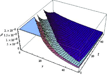
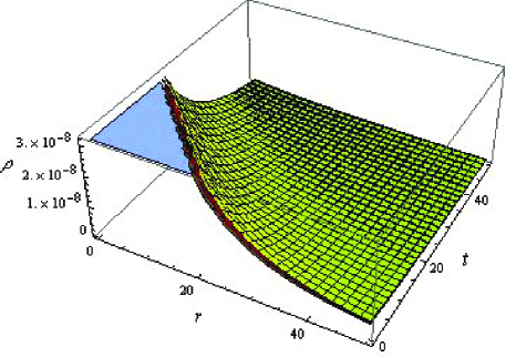
Figure 13: Plots of $\rho$ versus $r$ and $t$ for $\gamma=0.0001$, $\alpha=1$. The left graph is for $q=0$ (pink), $q=0.01$ (blue), $q=0.02$ (purple) with $\lambda=-0.001$ and the right graph is for $\lambda=-0.001$ (brown), $\lambda=-1$ (red), $\lambda=-2$ (yellow) with $q=0.01$.

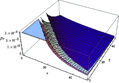
Figure 14: Plots of $p_{r}$ versus $r$ and $t$ for $\gamma=0.0001$, $\alpha=1$. The left graph is for $q=0$ (pink), $q=0.01$ (blue), $q=0.02$ (purple) with $\lambda=-0.001$ while the right graph is for $\lambda=-0.001$ (brown), $\lambda=-1$ (red), $\lambda=-2$ (yellow) with $q=0.01$.

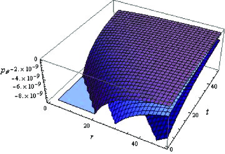
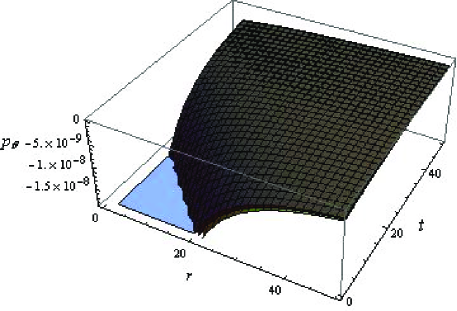
Figure 15: Plots of $p_{\theta}$ versus $r$ and $t$ for $\gamma=0.0001$, $\alpha=1$. The left graph is for $q=0$ (pink), $q=0.01$ (blue), $q=0.02$ (purple) with $\lambda=-0.001$ while the right graph is for $\lambda=-0.001$ (brown), $\lambda=-1$ (red), $\lambda=-2$ (yellow) with $q=0.01$.

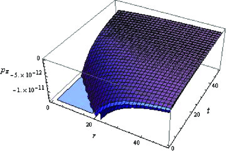
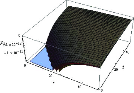
Figure 16: Plots of $p_{z}$ versus $r$ and $t$ for $\gamma=0.0001$, $\alpha=1$. The left graph is for $q=0$ (pink), $q=0.0001$ (blue), $q=0.0002$ (purple) with $\lambda=-0.001$ while the right graph is for $\lambda=-0.001$ (brown), $\lambda=-1$ (red), $\lambda=-2$ (yellow) with $q=0.01$.

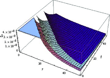
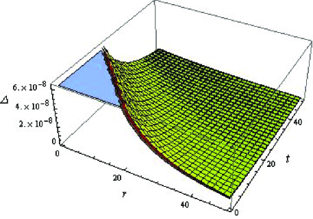
Figure 17: Plots of $\triangle$ versus $r$ and $t$ for $\gamma=0.0001$, $\alpha=1$. The left graph is for $q=0$ (pink), $q=0.01$ (blue), $q=0.02$ (purple) with $\lambda=-0.001$ while the right graph is for $\lambda=-0.001$ (brown), $\lambda=-1$ (red), $\lambda=-2$ (yellow) with $q=0.5$.

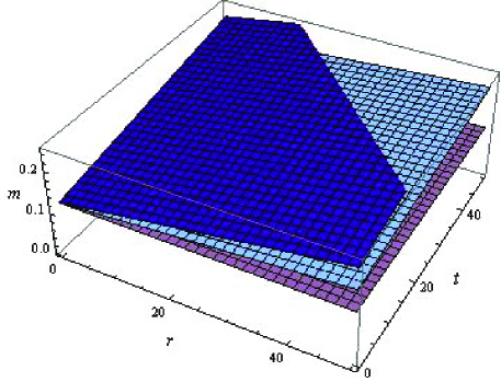
Figure 18: Plot of $m$ versus $r$ and $t$ for $\gamma=0.0001$, $\alpha=1$, $q=0$ (pink), $q=0.001$ (blue), $q=0.002$ (purple).

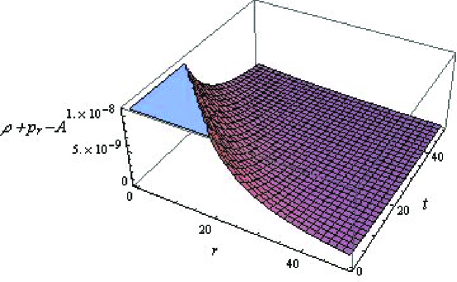
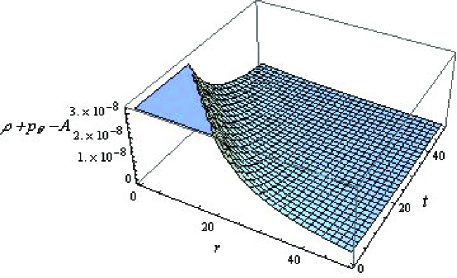
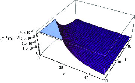
Figure 19: Plots for NEC for $\gamma=0.0001$, $\alpha=1$, $q=0.01$ and $\lambda=-0.001$.

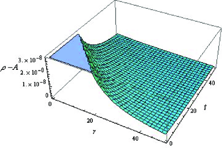
Figure 20: Plot for WEC for $\gamma=0.0001$, $\alpha=1$, $q=0.01$ and $\lambda=-0.001$.

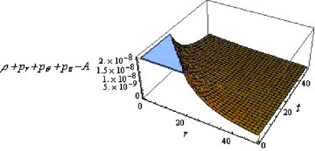
Figure 21: Plot for SEC for $\gamma=0.0001$, $\alpha=1$, $q=0.01$ and $\lambda=-0.001$.

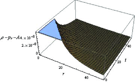
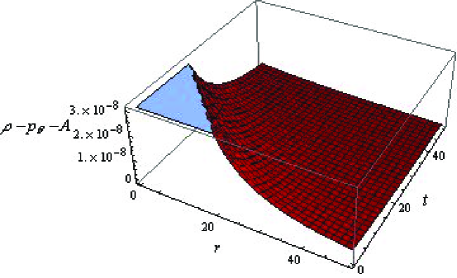
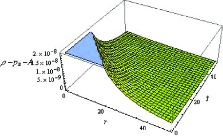
Figure 22: Plots for DEC for $\gamma=0.0001$, $\alpha=1$, $q=0.01$ and $\lambda=-0.001$.

4 Concluding Remarks

Accelerated expansion of the universe is an observed phenomenon which can affect astrophysical processes. To study the consequences of the expanding universe on collapsing and expanding scenarios of a stellar object, we consider charged anisotropic cylindrical source in $f(R,T)$ framework. The solutions of Einstein-Maxwell field equations governing the phenomena of collapse and expansion during stellar evolution are discussed. We explore the role of electromagnetic field and model parameter on the physical features.

In case of collapse solution, the expansion scalar, density, pressures ($p_{r},~{}p_{\theta}$ and $p_{z}$), anisotropy and mass do not change with radial coordinate. For expanding solution, the change remains the same for both coordinates. The behavior of these parameters with respect to time remains the same for both cases, except $p_{z}$. The anisotropy is positive for both cases which enhances the compactness of the system as discussed in [36]. In both cases, the increase in total charge has the same effects on physical quantities. The effects of model parameter is different for $p_{\theta}$ and $p_{z}$ in both cases while it is same for the remaining quantities. We conclude that the collapse rate increases for the collapse solution while the expansion rate decreases for the expanding solution. It is found that the energy conditions are satisfied in both cases showing physical viability of our solutions for the considered values of constants.

Finally, we compare our results with those found in GR or $\lambda=0$ [29]. For our collapse solution, the change in physical quantities is related with increase in time not with radius while in GR the quantities vary with radial coordinate but do not vary with temporal one. In case of expanding cylinder, the physical parameters vary with increase in both time and radius for our solution while in GR the solution only induces a change with respect to $t$. In both cases, the anisotropy decreases for our solutions while it increases in GR. The increase in anisotropy can distort the geometry of the system, i.e., solutions in GR can deform the shape of the system. On the other hand, for our solutions the anisotropy decreases leading to geometry preservation which is due to the dark source terms. It is worthwhile to mention here that our solutions satisfy the energy condition for chosen values of constants which are not shown in the similar works [26]-[29].

Acknowledgment

We would like to thank the Higher Education Commission, Islamabad, Pakistan for its financial support through the Indigenous Ph.D. 5000 Fellowship Program Phase-II, Batch-III.

References

• [1] Oppenheimer, J.R. and Snyder, H.: Phys. Rev. 56(1939)455.
• [2] Misner, C.W., Sharp, D.: Phys. Rev. 136(1964)B571.
• [3] Misner, C.W., Sharp, D.H.: Phys. Lett. 15(1965)279.
• [4] Stark, R.F. and Piran, T.: Phys. Rev. Lett. 55(1985)891.
• [5] Herrera, L., Santos, N.O. and Le Denmat, G.: Mon. Not. R. Astron. Soc. 237(1989)257.
• [6] Harada, T: Phys. Rev. D 58(1998)104015.
• [7] Joshi, P.S. and Dwivedi, I.H.: Class. Quantum Grav. 16(1999)41.
• [8] Sharif, M. and Kausar, H.R.: Astrophys. Space. Sci. 331(2011)281.
• [9] Cembranos, J.A.R., Cruz-Dombriz, A.D.L. and NΓΊez, B.M.: J. Cosmol. Astropart. Phys. 04(2012)021.
• [10] Kausar, H.R., Philippoz, L. and Jetzer, P.: Phys. Rev. D 93(2016)124071.
• [11] Harko, T., Lobo, F.S.N., Nojiri, S. and Odintsov, S.D.: Phys. Rev. D 84(2011)024020.
• [12] Harko, T. and Lobo, F.S.N.: Galaxies 2(2014)410.
• [13] Shabani, H. and Farhoudi, M.: Phys. Rev. D 90(2014)044031.
• [14] Moraes, P.H.R.S.: Eur. Phys. J. C 75(2015)168.
• [15] Noureen, I. and Zubair, M.: Astrophys. Space Sci. 356(2015)103.
• [16] Carvalho, G.A. et al.: Eur. Phys. J. C 77(2017)871.
• [17] Sharif, M. and Bhatti, M.Z.: J. Cosmol. Astropart. phys. 10(2013)056.
• [18] Yousaf, Z., Bhatti, M.Z. and Farwa, U.: Class. Quantum Grav. 34(2017)145002.
• [19] Sharif, M. and Farooq, N.: Eur. Phys. J. Plus 132(2017)355.
• [20] Sharif, M. and Farooq, N.: Int. J. Mod. Phys. D 27(2018)1850013.
• [21] Rosseland, S. and Eddington, A.S.: Mon. Not. R. Astron. Soc. 84(1924)720.
• [22] Bonnor, W.B.: Mon. Not. R. Astron. Soc. 129(1964)443.
• [23] Azam, M., Mardan, S.A. and Rehman, M.A.: Adv. High Energy Phys. 2015(2015)865086.
• [24] Bhatti, M.Z. and Yousaf, Z.: Eur. Phys. J. C 76(2016)219.
• [25] Mansour, H., Lakhal, B. Si and Yanallah, A.: J. Cosmol. Astropart. Phys. 06(2018)006.
• [26] Glass, E.N.: Gen. Relativ. Gravit. 45(2013)266.
• [27] Abbas, G.: Astrophys. Space Sci. 350(2014)307.
• [28] Abbas, G.: Astrophys. Space Sci. 352(2014)955.
• [29] Abbas, G.: Astrophys. Space Sci. 357(2015)56.
• [30] Abbas, G. and Ahmed, R.: Eur. Phys. J. C 77(2017)441.
• [31] Sharif, M. and Siddiqa A.: Int. J. Mod. Phys. DOI: 10.1142/S0218271819500044 (2019).
• [32] Moraes, P.H.R.S.: Eur. Phys. J. C 75(2015)168; Correa, R.A.C. and Moraes, P.H.R.S.: Eur. Phys. J. C 76(2016)100; Das, A., Rahaman, F., Guha, B.K. and Ray, S.: Eur. Phys. J. C 76(2016)654; Das, A., Ghosh, S., Guha, B.K., Das, S., Rahaman, F. and Ray, S.: Phys. Rev. D 95(2017)124011.
• [33] Poplawski, N.J.: arXiv:gr-qc/0608031.
• [34] Misner, C.W. and Sharp, D.: Phys. Rev. B 137(1965)96501360.
• [35] Sharif, M. and Ikram, A.: Int. J. Mod. Phys. D 27(2018)1750182.
• [36] Maurya, S.K., Ray, S., Ghosh, S., Manna, S. and Smitha T.T.: Ann. Phys. 395(2018)152.