Faster arbitrary-precision dot product and matrix multiplication

Abstract

We present algorithms for real and complex dot product and matrix multiplication in arbitrary-precision floating-point and ball arithmetic. A low-overhead dot product is implemented on the level of GMP limb arrays; it is about twice as fast as previous code in MPFR and Arb at precision up to several hundred bits. Up to 128 bits, it is 3-4 times as fast, costing 20-30 cycles per term for floating-point evaluation and 40-50 cycles per term for balls. We handle large matrix multiplications even more efficiently via blocks of scaled integer matrices. The new methods are implemented in Arb and significantly speed up polynomial operations and linear algebra.

I Introduction

The dot product and matrix multiplication are core building blocks for many numerical algorithms. Our goal is to optimize these operations in real and complex arbitrary-precision arithmetic. We treat both floating-point arithmetic and ball arithmetic [21] in which errors are tracked rigorously using midpoint-radius $[m\pm r]$ intervals. Our implementations are part of the open source (LGPL) Arb library [14] (http://arblib.org/) as of version 2.16.

In this work, we only consider CPU-based software arithmetic using GMP [7] for low-level operations on mantissas represented by arrays of 32-bit or 64-bit words (limbs). This is the format used in MPFR [5] as well as Arb. The benefit is flexibility (we handle mixed precision from few bits to billions of bits); the drawback is high bookkeeping overhead and limited vectorization opportunities. In “medium” precision (up to several hundred bits), arithmetic based on floating-point vectors (such as double-double and quad-double arithmetic) offers higher performance on modern hardware with wide SIMD floating-point units (inluding GPUs) [11, 22, 15]. However, such formats typically give up some flexibility (having a limited exponent range, usually assuming a fixed precision for all data).

The MPFR developers recently optimized arithmetic for same-precision operands up to 191 bits [17]. In this work, we reach even higher speed without restrictions on the operands by treating a whole dot product as an atomic operation. This directly speeds up many “basecase” algorithms expressible using dot products, such as classical $O(N^{2})$ polynomial multiplication and division and $O(N^{3})$ matrix multiplication. Section III describes the new dot product algorithm in detail.

For large polynomials and matrices (say, of size $N>50$), reductions to fast polynomial and matrix multiplication are ultimately more efficient than iterated dot products. Section IV looks at fast and accurate matrix multiplication via scaled integer matrices. Section V presents benchmark results and discusses the combination of small-$N$ and large-$N$ algorithms for polynomial operations and linear algebra.

II Precision and accuracy goals

Throughout this text, $p\geq 2$ denotes the output target precision in bits. For a dot product $\smash{s=\sum_{i=0}^{N-1}x_{i}y_{i}}$ where $x_{i},y_{i}$ are floating-point numbers (not required to have the same precision), we aim to approximate $s$ with error of order $\smash{\varepsilon\sim 2^{-p}\sum_{i=0}^{N-1}|x_{i}y_{i}|}$. In a practical sense, this accuracy is nearly optimal in $p$-bit arithmetic; up to cancellations that are unlikely for generic data, uncertainty in the input will typically exceed $\varepsilon$. Since $p$ is arbitrary, we can set it to (say) twice the input precision for specific tasks such as residual calculations. To guarantee an error of $\smash{2^{-p}s}$ or even $p$-bit correct rounding of $s$, we may do a fast calculation as above with (say) $p+20$ bits of precision and fall back to a slower correctly rounded summation [18] only when the fast dot product fails.

A dot product in ball arithmetic becomes

$$\textstyle{\sum_{i=0}^{N-1}[m_{i}\pm r_{i}][m^{\prime}_{i}\pm r^{\prime}_{i}]\subseteq[m\pm r],}$$

$$\textstyle{m\!=\!\sum_{i=0}^{N-1}\!m_{i}m^{\prime}_{i}+\varepsilon,\,r\geq|\varepsilon|+\sum_{i=0}^{N-1}\!|m_{i}|r^{\prime}_{i}\!+\!|m^{\prime}_{i}|r_{i}\!+\!r_{i}r^{\prime}_{i}}.\\$$

We compute $m$ with $p$-bit precision (resulting in some rounding error $\varepsilon$), and we compute a low-precision upper bound for $r$ that is tight up to rounding errors on $r$ itself. If the input radii $r_{i},r_{i}^{\prime}$ are all zero and the computation of $m$ is exact ($\varepsilon=0$), then the output radius $r$ will be zero. If $r$ is large, we can sometimes automatically reduce the precision without affecting the accuracy of the output ball.

We require that matrix multiplication give each output entry with optimal (up to cancellation) accuracy, like the classical algorithm of evaluating $N^{2}$ separate dot products. In particular, for a structured or badly scaled ball matrix like

$$\small\begin{pmatrix}[1.23\!\cdot\!10^{100}\pm 10^{80}]\!\!&-1.5&0\\ 1&\!\![2.34\pm 10^{-20}]\!&[3.45\pm 10^{-50}]\\ 0&2&\!\![4.56\cdot 10^{-100}\pm 10^{-130}]\end{pmatrix}\!,$$

we preserve small entries and the individual error magnitudes. Many techniques for fast multiplication sacrifice such information. Losing information is sometimes the right tradeoff, but can lead to disaster (for example, 100-fold slowdown [12]) when the input data is expensive to compute to high accuracy. Performance concerns aside, preserving entrywise information reduces the risk of surprises for users.

III Arbitrary-precision dot product

The obvious algorithm to evaluate a dot product $\sum_{i=0}^{N-1}x_{i}y_{i}$ performs one multiplication followed by $N-1$ multiplications and additions (or fused multiply-add operations) in a loop. The functions arb_dot, arb_approx_dot, acb_dot and acb_approx_dot were introduced in Arb 2.15 to replace most such loops. The function

void arb_dot(arb_t res, const arb_t initial, int sub,
    arb_srcptr x, long xstep, arb_srcptr y,
    long ystep, long N, long p)

sets res to a ball containing $\textstyle{\textit{initial}+(-1)^{\textit{sub}}\sum_{i=0}^{N-1}x_{i}\,y_{i}}$ where $x_{i}=[m_{i}\pm r_{i}]$, $y_{i}=[m_{i}^{\prime}\pm r_{i}^{\prime}]$ and initial are balls of type arb_t given in arrays with strides of xstep and ystep. The optional initial term (which may be NULL), sub flag and pointer stride lengths (which may be negative) permit expressing many common operations in terms of arb_dot without extra arithmetic operations or data rearrangement.

The approx version is similar but ignores the radii and computes an ordinary floating-point dot product over the midpoints, omitting error bound calculations. The acb versions are the counterparts for complex numbers. All four functions are based on Algorithm 1, which is explained in detail below.

III-A Representation of floating-point numbers

The dot product algorithm is designed around the representation of arbitrary-precision floating-point numbers and midpoint-radius intervals (balls) used in Arb. In the following, $\beta\in\{32,64\}$ is the word (limb) size, and $p_{\operatorname{rad}}=30$ is the radius precision, which is a constant.

An arb_t contains a midpoint of type arf_t and a radius of type mag_t. An arf_t holds one of the special values $0,\pm\infty,\operatorname{NaN}$, or a regular floating-point value

$$\textstyle{m=(-1)^{\textit{sign}}\cdot 2^{e}\cdot\sum_{k=0}^{n-1}b_{k}2^{\beta(k-n)}}$$ (1)

where $b_{k}$ are $\beta$-bit mantissa limbs normalized so that $2^{\beta-1}\leq b_{n-1}\leq 2^{\beta}-1$ and $b_{0}\neq 0$. Thus $n$ is always the minimal number of limbs needed to represent $x$, and we have $2^{e-1}\leq|m|<2^{e}$. The limbs are stored inline in the arf_t structure when $n\leq 2$ and otherwise in heap-allocated memory. The exponent $e$ can be arbitrarily large: a single word stores $|e|<2^{\beta-2}$ inline and larger $e$ as a pointer to a GMP integer.

A mag_t holds an unsigned floating-point value $0,+\infty$, or $r=(b/2^{p_{\operatorname{rad}}})2^{f}$ where $2^{p_{\operatorname{rad}}-1}\leq b<2^{p_{\operatorname{rad}}}$ occupies the low $p_{\operatorname{rad}}$ bits of one word. We have $2^{f-1}\leq|r|<2^{f}$, and as for arf_t, the exponent $f$ can be arbitrarily large.

The methods below can be adapted for MPFR with minimal changes. MPFR variables (mpfr_t) use the same representation as (1) except that a precision $p$ is stored in the variable, the number of limbs is always $n=\lceil p/\beta\rceil$ even if $b_{0}=0$, there is no $n\leq 2$ allocation optimization, the exponent $e$ cannot be arbitrarily large, and $-0$ is distinct from $+0$.

III-B Outline of the dot product

We describe the algorithm for $\emph{initial}=0$ and $\emph{sub}=0$. The general case can be viewed as extending the dot product to length $N+1$, with trivial sign adjustments.

The main observation is that each arithmetic operation on floating-point numbers of the form (1) has a lot of overhead for limb manipulations (case distinctions, shifts, masks), particularly during additions and subtractions. The remedy is to use a fixed-point accumulator for the whole dot product and only convert to a rounded and normalized floating-point number at the end. The case distinctions for subtractions are simplified by using two’s complement arithmetic. Similarly, we use a fixed-point accumulator for the radius dot product.

We make two passes over the data: the first pass inspects all terms, looks for exceptional cases, and determines an appropriate working precision and exponents to use for the accumulators. The second pass evaluates the dot product.

There are three sources of error: arithmetic error on the accumulator (tracked with one limb counting ulps), the final rounding error, and the propagated error from the input balls. At the end, the three contributions are added to a single $p_{\operatorname{rad}}$-bit floating-point number. The approx version of the dot product simply omits all these steps.

Except where otherwise noted, all quantities describing exponents, shift counts (etc.) are single-word ($\beta$-bit) signed integers between $\textit{MIN}=-2^{\beta-1}$ and $\textit{MAX}=2^{\beta-1}-1$, and all limbs are $\beta$-bit unsigned words.

Algorithm 1 Dot product in arbitrary-precision ball arithmetic: given $[m_{i}\pm r_{i}],[m^{\prime}_{i}\pm r^{\prime}_{i}],0\leq i<N$ and a precision $p\geq 2$, compute $[m\pm r]$ containing $\sum_{i=0}^{N-1}[m_{i}\pm r_{i}][m^{\prime}_{i}\pm r^{\prime}_{i}]$.

1:Setup: check unlikely cases (infinities, NaNs, overflow and underflow); determine exponent $e_{s}$ and number of limbs $n_{s}$ for the midpoint accumulator; determine exponent $e_{\operatorname{rad}}$ for the radius accumulator; reduce $p$ if possible. (See details below.)

2:Initialization: allocate temporary space; initialize accumulator limbs $s$: $s_{n_{s}-1},\ldots,s_{0}\leftarrow 0,\ldots,0$, one limb $\textit{err}\leftarrow 0$ for the ulp error on $s_{0}$, and a 64-bit integer $\textit{srad}\leftarrow 0$ as radius accumulator.

3:Evaluation: for each term $t=m_{i}m^{\prime}_{i}$, compute the limbs of $t$ that overlap with $s$, shift and add to $s$ (or two’s complement subtract if $t<0$), incrementing err if inexact. Add scaled upper bound for $|m_{i}|r^{\prime}_{i}+|m^{\prime}_{i}|r_{i}+r_{i}r_{i}^{\prime}$ to srad.

4:Finalization:

1. If $s_{n_{s}-1}\geq 2^{\beta-1}$, negate $s$ (one call to GMP’s mpn_neg) and set $\textit{sign}\leftarrow 1$, else set $\textit{sign}\leftarrow 0$.

2. $m\leftarrow(-1)^{\textit{sign}}\cdot 2^{e_{s}}\cdot(\sum_{k=0}^{n_{s}-1}s_{k}2^{\beta(k-n_{s})})$ rounded to $p$ bits, giving a possible rounding error $\varepsilon_{\text{round}}$.

3. $r\leftarrow\varepsilon_{\text{round}}+\textit{err}\cdot 2^{e_{s}-n_{s}\beta}+\textit{srad}\cdot 2^{e_{\operatorname{rad}}-p_{\operatorname{rad}}}$ as a floating-point number with $p_{\operatorname{rad}}$ bits (rounded up).

4. Free temporary space and output $[m\pm r]$.

III-C Setup pass

The setup pass in Algorithm 1 uses the following steps:

1. $N_{\operatorname{nonzero}}\leftarrow 0$ (number of nonzero terms).

2. $e_{\operatorname{max}}\leftarrow\textit{MIN}$ (upper bound for term exponents).

3. $e_{\operatorname{min}}\leftarrow\textit{MAX}$ (lower bound for content).

4. $e_{\operatorname{rad}}\leftarrow\textit{MIN}$ (upper bound for radius exponents).

5. For $0\leq i<N$:

   1. If any of $m_{i},m_{i}^{\prime},r_{i},r_{i}^{\prime}$ is non-finite or has an exponent outside of $\pm 2^{\beta-4}$ (unlikely), quit Algorithm 1 and use a fallback method.

   2. If $m_{i}$ and $m_{i}^{\prime}$ are both nonzero, with respective exponents $e,e^{\prime}$ and limb counts $n,n^{\prime}$:

      • Set $N_{\operatorname{nonzero}}\leftarrow N_{\operatorname{nonzero}}+1$.

      • Set $e_{\operatorname{max}}\leftarrow\max(e_{\operatorname{max}},\,e+e^{\prime})$.

      • If $p>2\beta$, $e_{\operatorname{min}}\leftarrow\min(e_{\operatorname{min}},\,e+e^{\prime}-\beta(n+n^{\prime}))$.

   3. For each product $|m_{i}|r_{i}^{\prime}$, $|m_{i}^{\prime}|r_{i}$, $r_{i}r_{i}^{\prime}$ that is nonzero, denote the exponents of the respective factors by $e,e^{\prime}$ and set $e_{\operatorname{rad}}\leftarrow\max(e_{\operatorname{rad}},e+e^{\prime})$.

6. If $e_{\operatorname{max}}\!=\!e_{\operatorname{rad}}\!=\!\textit{MIN}$, quit Algorithm 1 and output $[0\pm 0]$

7. (Optimize $p$.) If $e_{\operatorname{max}}=\textit{MIN}$, set $p\leftarrow 2$. Otherwise:

   1. If $e_{\operatorname{rad}}\neq\textit{MIN}$, set $p\leftarrow\min(p,e_{\operatorname{max}}-e_{\operatorname{rad}}+p_{\operatorname{rad}})$ (if the final radius $r$ will be larger than the expected arithmetic error, we can reduce the precision used to compute $m$ without affecting the accuracy of the ball $[m\pm r]$).

   2. If $e_{\operatorname{min}}\neq\textit{MAX}$, set $p\leftarrow\min(p,e_{\operatorname{max}}-e_{\operatorname{min}}+p_{\operatorname{rad}})$ (if all terms fit in a window smaller than $p$ bits, reducing the precision does not change the result).

   3. Set $p\leftarrow\max(p,2)$.

8. Set $\textit{padding}\leftarrow 4+\operatorname{bc}(N)$, where $\operatorname{bc}(\nu)=\lceil\log_{2}(\nu+1)\rceil$ denotes the binary length of $\nu$.

9. Set $\textit{extend}\leftarrow\operatorname{bc}(N_{\operatorname{nonzero}})+1$.

10. Set $n_{s}\leftarrow\max(2,\lceil(p+\textit{extend}+\textit{padding})/\beta\rceil)$.

11. Set $e_{s}\leftarrow e_{\operatorname{max}}+\textit{extend}$.

All terms $|m_{i}m_{i}^{\prime}|$ are bounded by $2^{e_{\operatorname{max}}}$ and similarly all radius terms are bounded by $2^{e_{\operatorname{rad}}}$. The width of the accumulator is $p$ bits plus extend leading bits and padding trailing bits, rounded up to a whole number of limbs $n_{s}$. The quantity extend guarantees that carries never overflow the leading limb $s_{n_{s}-1}$, including one bit for two’s complement negation; it is required to guarantee correctness. The quantity padding adds a few guard bits to enhance the accuracy of the dot product; this is an entirely optional tuning parameter.

III-D Evaluation

For a midpoint term $m_{i}m_{i}^{\prime}\neq 0$, denote the exponents of $m_{i},m_{i}^{\prime}$ by $e,e^{\prime}$ and the limb counts by $n,n^{\prime}$. The multiply-add operation uses the following steps.

1. Set $\textit{shift}\leftarrow e_{s}-(e+e^{\prime})$, $\textit{shift\_bits}\leftarrow\textit{shift}\bmod\beta$, $\textit{shift\_limbs}\leftarrow\lfloor\textit{shift}/\beta\rfloor$.

2. If $\textit{shift}\geq\beta n_{s}$, set $\textit{err}\leftarrow\textit{err}+1$ and go on to the next term (this term does not overlap with the limbs in $s$).

3. Set $p_{t}\leftarrow\beta n_{s}-\textit{shift}$ (effective bit precision needed for this term), and set $n^{\prime\prime}\leftarrow\lceil p_{t}/\beta\rceil+1$. If $n>n^{\prime\prime}$ or $n^{\prime}>n^{\prime\prime}$, set $\textit{err}\leftarrow\textit{err}+1$. (We read at most $n^{\prime\prime}$ leading limbs from $m$ and $m^{\prime}$ since the smaller limbs have a negligible contribution to the dot product; in case of truncation, we increment the error bound by 1 ulp.)

4. Set $n_{t}\leftarrow\min(n,n^{\prime\prime})+\min(n^{\prime},n^{\prime\prime})$. The term will be stored in up to $n_{t}+1$ temporary limbs $t_{n_{t}},\ldots,t_{0}$ pre-allocated in the initialization of Algorithm 1.

5. Set $t_{n_{t}-1},\ldots,t_{0}$ to the product of the top $\min(n,n^{\prime\prime})$ limbs of $m$ and the top $\min(n^{\prime},n^{\prime\prime})$ limbs of $m^{\prime}$ (this is one call to GMP’s mpn_mul). We now have the situation depicted in Figure 1.

6. (Bit-align the limbs.) If $\textit{shift\_bits}\neq 0$, set $t_{n_{t}},\ldots,t_{0}$ to $t_{n_{t}-1},\ldots,t_{0}$ right-shifted by shift_bits bits (this is a pointer adjustment and one call to mpn_rshift) and then set $n_{t}\leftarrow n_{t}+1$.

7. (Strip trailing zero limbs.) While $t_{0}=0$, increment the pointer to $t$ and set $n_{t}\leftarrow n_{t}-1$.

Figure 1: The accumulator $s_{n_{s}-1},\ldots,s_{0}$ and the term $t_{n_{t}-1},\ldots,t_{0}$, prior to limb alignment. More significant limbs are shown towards the left.

It remains to add the aligned limbs of $t$ to the accumulator $s$. We have two cases, with $v$ denoting the number of overlapping limbs between $s$ and $t$ and $d_{s}$ and $d_{t}$ denoting the offsets from $s_{0}$ and $t_{0}$ to the overlapping segment. If $\textit{shift\_limbs}+n_{t}\leq n_{s}$ (no discarded limbs), set $d_{s}\leftarrow n_{s}-\textit{shift\_limbs}-n_{t}$, $d_{t}\leftarrow 0$ and $v\leftarrow n_{t}$. Otherwise, set $d_{s}\leftarrow 0$, $d_{t}\leftarrow n_{t}-n_{s}+\textit{shift\_limbs}$, $v\leftarrow n_{s}-\textit{shift\_limbs}$ and $\textit{err}\leftarrow\textit{err}+1$. The addition is now done using the GMP code

cy = mpn_add_n(s + ds, s + ds, t + dt, v);
mpn_add_1(s + ds + v, s + ds + v, shift_limbs, cy);

if $m_{i}m_{i}^{\prime}>0$, or in case $m_{i}m_{i}^{\prime}<0$ using mpn_sub_n and mpn_sub_1 to perform a two’s complement subtraction.

Our code has two more optimizations. If $n\leq 2,n^{\prime}\leq 2$, $n_{s}\leq 3$, the limb operations are done using inline code instead of calling GMP functions, speeding up precision $p\leq 128$ (on 64-bit machines). When $p_{t}\geq 25\beta$ and $\min(n,n^{\prime})\beta>0.9p_{t}$, we compute $n^{\prime\prime}$ leading limbs of the product using the MPFR-internal function mpfr_mulhigh_n instead of mpn_mul. This is done with up to 1 ulp error on $s_{0}$ and is therefore accompanied by an extra increment of err.

III-E Radius operations

For the radius dot product $\sum_{i=0}^{N-1}|m_{i}|r^{\prime}_{i}+|m^{\prime}_{i}|r_{i}+r_{i}r_{i}^{\prime}$, we convert the midpoints $|m_{i}|$, $|m^{\prime}_{i}|$ to upper bounds in the radius format $r=(b/2^{p_{\operatorname{rad}}})2^{e}$ by taking the top $p_{\operatorname{rad}}$ bits of the top limb and incrementing; this results in the weakly normalized mantissa $2^{p_{\operatorname{rad}}-1}\leq b\leq 2^{p_{\operatorname{rad}}}$. The summation is done with an accumulator $(\textit{srad}/2^{p_{\operatorname{rad}}})2^{e_{\operatorname{rad}}}$ where srad is one unsigned 64-bit integer (1 or 2 limbs). The step to add an upper bound for $(a/2^{p_{\operatorname{rad}}})(b/2^{p_{\operatorname{rad}}})2^{e}$ is $\textit{srad}\leftarrow\textit{srad}+\lfloor(ab)/2^{p_{\operatorname{rad}}+e_{\operatorname{rad}}-e}\rfloor+1$ if $e_{\operatorname{rad}}-e<p_{\operatorname{rad}}$ and $\textit{srad}\leftarrow\textit{srad}+1$ otherwise.

By construction, $e_{\operatorname{rad}}\geq e$, and due to the 34 free bits for carry accumulation, srad cannot overflow if $N<2^{32}$. (Larger $N$ could be supported by increasing $e_{\operatorname{rad}}$, at the cost of some loss of accuracy.) We use conditionals to skip zero terms; the radius dot product is therefore evaluated as zero whenever possible, and if the input balls are exact, no radius computations are done apart from inspecting the terms.

III-F Complex numbers

Arb uses rectangular “balls” $[a\pm r]+[b\pm s]i$ to represent complex numbers. A complex dot product is essentially performed as two length-$2N$ real dot products. This preserves information about whether real or imaginary parts are exact or zero, and both parts can be computed with high relative accuracy when they have different scales. The algorithm could be adapted in the obvious way for true complex balls (disks).

For terms where both real and imaginary parts have similar magnitude and high precision, we use the additional optimization of avoiding one real multiplication via the formula

$$(a+bi)(c+di)=ac-bd+i[(a+b)(c+d)-ac-bd].$$ (2)

Since this formula is applied exactly and only for the midpoints, accuracy is not compromised. The cutoff occurs at the rather high 128 limbs (8192 bits) since (2) is implemented using exact products and therefore competes against mulhigh; an improvement is possible by combining mulhigh with (2).

IV Matrix multiplication

We consider the problem of multiplying an $M\times N$ ball matrix $[A\pm R_{A}]$ by an $N\times K$ ball matrix $[B\pm R_{B}]$ (where $R_{A},R_{B}$ are nonnegative matrices and $[\pm]$ is interpreted entrywise). The classical algorithm can be viewed as computing $MP$ dot products of length $N$. For large matrices, it is better to convert from arbitrary-precision floating-point numbers to integers [21]. Integer matrices can be multiplied efficiently using multimodular techniques, working modulo several word-size primes followed by Chinese remainder theorem reconstruction. This saves time since computations done over a fixed word size have less overhead than arbitrary-precision computations. Moreover, for modest $p$, the running time essentially scales as $O(p)$ compared to the $O(p^{2})$ with dot products, as long as the cost of the modular reductions and reconstructions does not dominate. The downside of converting floating-point numbers to integers is that we either must truncate entries (losing accuracy) or zero-pad (losing speed).

Our approach to matrix multiplication resembles methods for fast and accurate polynomial multiplication discussed in previous work [20],[14]. For polynomial multiplication, Arb scales the inputs and converts the coefficients to integers, adaptively splitting the polynomials into smaller blocks to keep the height of the integers small. The integer polynomials are then multiplied using FLINT [10], which selects between classical, Karatsuba and Kronecker algorithms and an asymptotically fast Schönhage-Strassen FFT. Arb implements other operations (such as division) via methods such as Newton iteration that asymptotically reduce to polynomial multiplication.

In this section, we describe an approach to multiply matrices in Arb following similar principles. We compute $[A\pm R_{A}][B\pm R_{B}]$ using three products $AB$, $|A|R_{B}$, $R_{A}(|B|+R_{B})$ where we use FLINT integer matrices for the high-precision midpoint product $AB$. FLINT in turn uses classical multiplication, the Strassen algorithm, a multimodular algorithm employing 60-bit primes, and combinations of these methods. An important observation for both polynomials and matrices is that fast algorithms such as Karatsuba, FFT and Strassen multiplication do not affect accuracy when used on the integer level.

Figure 2: Matrix multiplication $C=AB$ using scaled blocks.

IV-A Splitting and scaling

The earlier work by van der Hoeven [21] proposed multiplying arbitrary-precision matrices via integers truncated to $p$-bit height, splitting size-$N$ matrices into $m^{2}$ blocks of size $N/m$, where the user selects $m$ to balance speed and accuracy. Algorithm 2 improves on this idea by using a fully automatic and adaptive splitting strategy that guarantees near-optimal entrywise accuracy (like the classical algorithm).

Algorithm 2 Matrix multiplication using blocks: given ball matrices $[A\pm R_{A}]$, $[B\pm R_{B}]$ and a precision $p\geq 2$, compute $[C\pm R_{C}]$ containing $[A\pm R_{A}][B\pm R_{B}]$

1:$[C\pm R_{C}]\leftarrow[0\pm 0]$ $\triangleright$ Initialize the zero matrix

2:$h\leftarrow 1.25\min(p,\max(p_{A},p_{B}))\!+\!192$, where $p_{M}$ is the minimum floating-point precision needed to represent all entries of $M$ exactly $\triangleright$ Height bound tuning parameter

3:$S\leftarrow\{0,\ldots,N-1\}$ where $N$ is the inner dimension

4:while $S\neq\{\}$ do

5:     Extract $s\subseteq S$ such that $|E_{s}A_{s}|<2^{h}$ and $|B_{s}F_{s}|<2^{h}$

6:     if $\operatorname{size}(s)<30$ then $\triangleright$ Basecase for short blocks

7:         Extend $s$ to $\min(30,\operatorname{size}(S))$ indices

8:         $[C\pm R_{C}]\leftarrow[C\pm R_{C}]+A_{s}B_{s}$ (using dot products)

9:     else

10:         $T\leftarrow(E_{s}A_{s})(B_{s}F_{s})$ $\triangleright$ Matrix product over $\mathbb{Z}$

11:         $[C\pm R_{C}]\leftarrow[C\pm R_{C}]+E_{s}^{-1}TF_{s}^{-1}$ $\triangleright$ Ball addition, with possible rounding error on $C$ added to $R_{C}$

12:     end if

13:     $S\leftarrow S\setminus s$

14:end while

15:Compute $R_{1}=|A|R_{B}$ and $R_{2}=R_{A}(|B|+R_{B})$ by splitting and scaling into blocks of double as above (but using floating-point arithmetic with upper bounds instead of ball arithmetic), and set $R_{C}\leftarrow R_{C}+R_{1}+R_{2}$

16:Output $[C\pm R_{C}]$

We split $A$ into column submatrices $A_{s}$ and $B$ into row submatrices $B_{s}$, where $s$ is some subset of the indices. For any such $A_{s}$, and for each row index $i$, let $e_{i,s}$ denote the unique scaling exponent such that row $i$ of $2^{e_{i,s}}A_{s}$ consists of integers of minimal height ($e_{i,s}$ is uniquely determined unless row $i$ of $A_{s}$ is identically zero, in which case we may take $e_{i,s}=0$). Similarly let $f_{j,s}$ be the optimal scaling exponent for column $j$ of $B_{s}$. Then the contribution of $A_{s}$ and $B_{s}$ to $C=AB$ consists of $E_{s}^{-1}((E_{s}A_{s})(B_{s}F_{s}))F_{s}^{-1}$ where $E_{s}=\operatorname{diag}(2^{e_{i,s}})$ scales the rows of $A_{s}$ and $F_{s}=\operatorname{diag}(2^{f_{i,s}})$ scales the columns of $B_{s}$ (see Figure 2), and where we may multiply $(E_{s}A_{s})(B_{s}F_{s})$ over the integers.

Crucially, only magnitude variations within rows of $A_{s}$ (columns of $B_{s}$) affect the height; the rows of $A_{s}$ can have different magnitude from each other (and similarly for $B_{s}$).

We extract indices $s$ by performing a greedy search in increasing order, appending columns to $A_{s}$ and rows to $B_{s}$ as long as a height bound is satisfied. The tuning parameter $h$ balances the advantage of using larger blocks against the disadvantage of using larger zero-padded integers. In the common case where both $A$ and $B$ are uniformly scaled and have the same (or smaller) precision as the output, one block product is sufficient. One optimization is omitted from the pseudocode: we split the rectangular matrices $E_{s}A_{s}$ and $B_{s}F_{s}$ into roughly square blocks before carrying out the multiplications. This reduces memory usage for the temporary integer matrices and can reduce the heights of the blocks.

We compute the radius products $|A|R_{B}$ and $R_{A}(|B|+R_{B})$ (where $|A|$ and $|B|$ are rounded to $p_{\textrm{rad}}$ bits) via double matrices, using a similar block strategy. The double type has a normal exponent range of $-1022$ to $1023$, so if we set $h=900$ and center $E_{s}A_{s}$ and $B_{s}F_{s}$ on this range, no overflow or underflow can occur. In practice a single block is sufficient for most matrices arising in medium precision computations.

IV-B Improvements

Algorithm 2 turns out to perform reasonably well in practice when many blocks are used, but it could certainly be improved. The bound $h$ could be tuned, and the greedy strategy to select blocks is clearly not always optimal. Going even further, we could extract non-contiguous submatrices, add an extra inner scaling matrix $G_{s}G_{s}^{-1}$ for the columns of $A_{s}$ and rows of $B_{s}$, and combine scaling with permutations. Finding the best strategy for badly scaled or structured matrices appears to be a difficult problem. There is some resemblance to the balancing problem for eigenvalue algorithms [16].

Both Algorithm 2 and the analogous algorithm used for polynomial multiplication in Arb have the disadvantage that all input bits are used, unlike classical multiplication based on Algorithm 1 which omits negligible limbs. This important optimization for non-uniform polynomials (compare [20]) and matrices should be considered in future work.

IV-C Complex matrices

We multiply complex matrices using four real matrix multiplications $(A+Bi)(C+Di)=(AC-BD)+(AD+BC)i$ outside of the basecase range for using complex dot products. An improvement would be to use (2) to multiply the midpoint matrices when all entries are uniformly scaled; (2) could also be used for blocks with a splitting and scaling strategy that considers the real and imaginary parts simultaneously.

V Benchmarks

Except where noted, the following results were obtained on an Intel i5-4300U CPU using GMP 6.1, MPFR 4.0, MPC 1.1 [4] (the complex extension of MPFR), QD 2.3.22 [11] (106-bit double-double and 212-bit quad-double arithmetic), Arb 2.16, and the December 2018 git version of FLINT.

V-A Single dot products

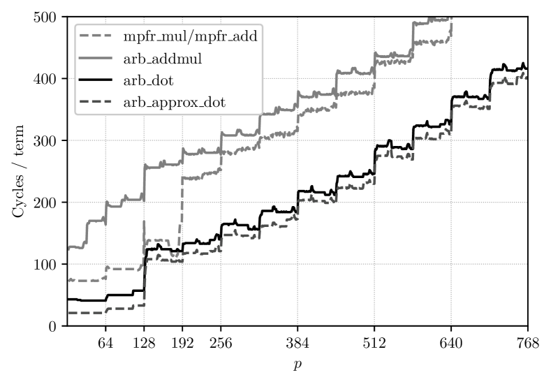
Figure 3: Dot product cost (cycles/term) as a function of the precision $p$, using MPFR, simple Arb code (arb_addmul in a loop), and Algorithm 1 in Arb (both ball and approximate floating-point versions).

Figure 3 and Table I show timings measured in CPU cycles per term for a dot product of length $N=100$ with uniform $p$-bit entries. We compare a simple loop using QD arithmetic, three MPFR versions, a simple Arb loop (addmul denoting repeated multiply-adds with arb_addmul), and Algorithm 1 in Arb, both for balls (dot denoting arb_dot) and floating-point numbers (approx denoting arb_approx_dot). Similarly, we include results for complex dot products, comparing MPC and three Arb methods. The mul/add MPFR version uses mpfr_mul and mpfr_add, with a preallocated temporary variable; fma denotes multiply-adds with mpfr_fma; our sum code writes exact products to an array and calls mpfr_sum [18] to compute the sum (and hence the dot product) with correct rounding. We make several observations:

• The biggest improvement is seen for $p\leq 128$ (up to two limbs). The ball dot product is up to 4.2 times faster than the simple Arb loop (and 2.0 times faster than MPFR); the approx version is up to 3.7 times faster than MPFR.

• A factor 1.5 to 2.0 speedup persists up to several hundred bits, and the speed for very large $p$ is close to the optimal throughput for GMP-based multiplication.

• Ball arithmetic error propagation adds 20 cycles/term overhead, equivalent to a factor 2.0 when $p\leq 128$ and a negligible factor at higher precision.

• At $p=106$, the approx dot product is about as fast as QD double-double arithmetic, while the ball version is half as fast; at $p=212$, either version is twice as fast as QD quad-double arithmetic.

• Complex arithmetic costs quite precisely four times more than real arithmetic. The speedup of our code compared to MPC is even greater than compared to MPFR.

• A future implementation of a correctly rounded dot product for MPFR and MPC using Algorithm 1 with mpfr_sum as a fallback should be able to achieve nearly the same average speed as the approx Arb version.

TABLE I: Cycles/term to evaluate a dot product ($N=100$).

	QD	MPFR (real)			Arb (real)
$p$		​​mul/add	fma	sum	​​addmul	dot	​​approx
53		74	99	108	169	40	20
106	26	97	156	124	203	49	27
159		140	183	169	257	123	105
212	265	237	208	188	277	133	117
424		350	288	288	374	215	201
848		670	619	597	705	522	499
1696		1435	1675	1667	1823	1471	1451
3392		4059	4800	4741	4875	3906	3880
​​13568		​33529	​39546	​39401	​39275	​32476	​32467
		MPC (complex)			Arb (complex)
$p$		​​mul/add			​​addmul	dot	​​approx
53		570			772	166	84
106		885			911	208	112
159		1016			1243	499	419
212		1123			1346	555	478
424		1591			1735	882	775
848		2803			3054	2097	2045
1696		8355			6953	5889	5821
3392		​18527			​17926	​15691	​15618
​​13568		​​129293			​​127672	​​125757	​​125634

TABLE II: Cycles/term to evaluate a dot product, variable $N$.

	Arb (real), dot				Arb (real), approx
$p$	$\!\!N\!=\!2$	$\!\!\!\!N\!=\!4$	$\!\!\!\!N\!=\!8$	$\!\!\!\!N\!=\!16$	$\!\!\!N\!=\!2$	$\!\!\!\!N\!=\!4$	$\!\!\!\!N\!=\!8$	$\!\!\!\!N\!=\!16$
53	89	65	53	44	64	41	31	23
106	98	75	61	53	71	47	37	31
212	215	175	159	143	177	147	136	125
848	614	571	552	535	567	547	522	507

For small $N$, the initialization and finalization overhead in Algorithm 1 is significant. Table II shows that it nevertheless performs better than a simple loop already for $N=2$ and quickly converges to the speed measured at $N=100$.

Algorithm 1 does even better with structured data, for example when the balls are exact, with small-integer coefficients, or with varying magnitudes. As an example of the latter, with $N=1000$, $p=1024$, and terms $(1/i!)\cdot(\pi^{-i})$, Algorithm 1 takes 0.035 ms while an arb_addmul loop takes 0.33 ms.

V-B Basecase polynomial and matrix operations

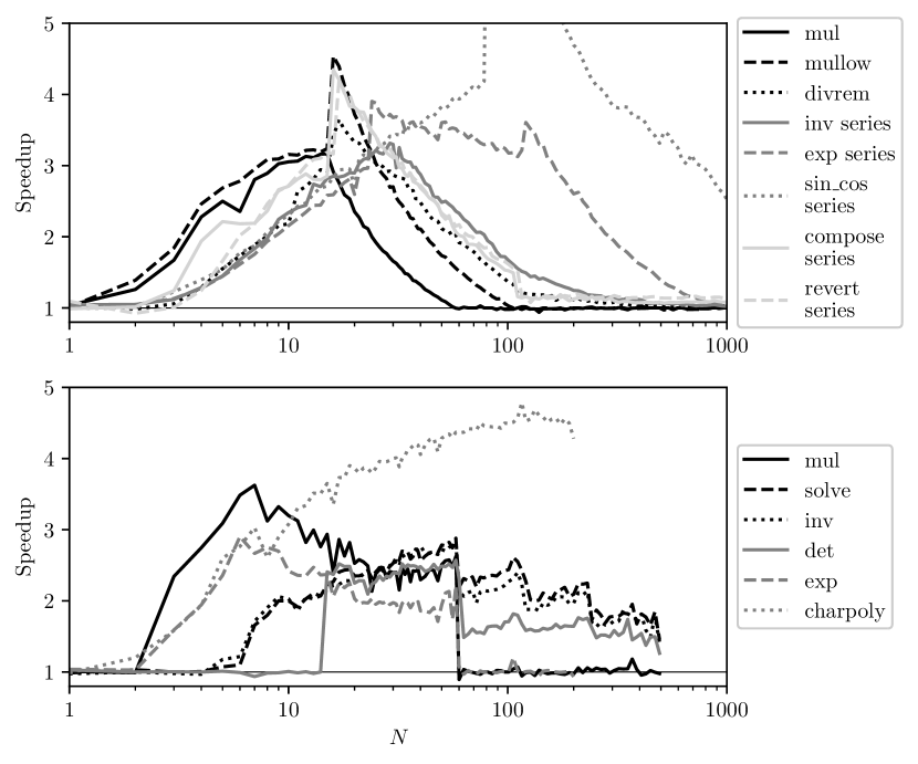
Figure 4: Speedup of Arb 2.15 over 2.14 for various operations on polynomials (top) and matrices (bottom), here for $p=64$ and complex coefficients.

The new dot product code was added in Arb 2.15 along with re-tuned cutoffs between small-$N$ and large-$N$ algorithms. Figure 4 shows the speedup of Arb 2.15 over 2.14 for operations on polynomials and power series of length $N$ and matrices of size $N$, here for $p=64$ and complex coefficients.

This shows the benefits of Algorithm 1, even in the presence of a fast large-$N$ algorithm (the block algorithm for matrix multiplication was added in Arb 2.14). The speedup typically grows with $N$ as the dot product gains an increasing advantage over a simple multiply-add loop, up to the old cutoff point for switching to a large-$N$ algorithm. To the right of this point, the dot product then gives a diminishing speedup over the large-$N$ algorithm up to the new cutoff. Jumps are visible where the old cutoff was suboptimal. We make some more observations:

• The speedup around $N\approx$ 10 to 30 is notable since this certainly is a common size for real-world use.

• Some large-$N$ algorithms like Newton iteration series inversion and block recursive linear solving use recursive operations of smaller size, so the improved basecase gives an extended “tail” speedup into the large-$N$ regime.

• The power series exponential and sine/cosine improve dramatically. The large-$N$ method uses Newton iteration which costs several polynomial multiplications, while the $O(N^{2})$ basecase method uses the dot product-friendly recurrence $\exp(a_{1}x+a_{2}x^{2}+\ldots)=b_{0}+b_{1}x+b_{2}x^{2}+\ldots$, $b_{0}=1$, $b_{k}=(\sum_{j=1}^{k}(ja_{j})b_{k-j})/k$. The cutoffs have been increased to $N=750$ and $N=1400$ (for this $p$).

• The characteristic polynomial (charpoly) does not currently use matrix multiplication in Arb, so we get the pure dot product speedup for large $N$.

• Series composition and reversion use baby-step giant-steps methods [2, 13] where dot products enter in both length-$N$ polynomial and size-$\!\sqrt{\!N}$ matrix multiplications.

V-C Large-$N$ matrix multiplication

TABLE III: Time (s) to multiply size-$N$ matrices. (#) is the number of blocks $A_{s}B_{s}$ used by the block algorithm, where greater than one.

	Uniform real				Pascal		Uniform complex
$p$	QD	MPFR​​	Arb​​​​​	Arb	Arb​​​​​	Arb	MPC​​	Arb	Arb
			dot	block	dot	block		dot	block​​​
$N=100$
53		0.035​​	0.019	0.0041​	0.016	0.021	0.28	0.071​​	0.017​​
106	0.011​​	0.042​​	0.023	0.011	0.018	0.031	0.40	0.086​​	0.049​​
212	0.11​​	0.11	0.061	0.021	0.063	0.046	0.50	0.23	0.092​​
848		0.30	0.23	0.089	0.23	0.12	1.2	0.85	0.34
​​3392		1.7	1.7	0.48	1.7	0.55	7.1	6.1	1.9
$N=300$
53		0.96	0.51	0.13	0.37	0.57 (3)​	8.1	2.0	0.37
106	0.30	1.2	0.69	0.23	0.47	0.70 (3)​	12	2.6	0.87
212	3.0	3.0	2.2	0.34	1.8	1.2 (3)​	14	7.5	1.5
848		7.9	6.2	1.2	5.1	2.4 (2)​	33	26	4.9
​​3392		46	47	6.0	44	7.3	200	172	24
$N=1000$
53		36	19	3.6	12	20 (10)​	313	75	14
106	11	44	25	5.6	14	23 (10)​	454	97	22
212	111	110	76	8.2	43	35 (9)​	539	342	33
848		293	258	27	122	80 (5)​	1230​​	1074​​	107
​​3392		1725​​	1785	115	1280	226 (2)​	7603​​	6789​​	457

Table III shows timings to compute $A\cdot A$ where $A$ is a size-$N$ matrix. We compare two algorithms in Arb (both over balls): dot is classical multiplication using iterated dot products, and block is Algorithm 2. The default matrix multiplication function in Arb 2.16 uses the dot algorithm for $N\leq 40$ to $60$ (depending on $p$) and block for larger $N$; for the sizes of $N$ in the table, block is always the default. We also time QD, MPFR and MPC classical multiplication (with two basic optimizations: tiling to improve locality, and preallocating a temporary inner variable for MPFR and MPC).

We test two kinds of matrices. The uniform $A$ is a matrix where all entries have similar magnitude. Here, the block algorithm only uses a single block and has a clear advantage; at $N=1000$, it is 5.3 times as fast as the classical algorithm when $p=53$ and 16 times as fast when $p=3392$.

The Pascal matrix $A$ has entries $\pi\cdot{i+j\choose i}$ which vary in magnitude between unity and $4^{N}$. This is a bad case for Algorithm 2, requiring many blocks when $N$ is much larger than $p$. Conversely, the classical algorithm is faster for this matrix than for the uniform matrix since Algorithm 1 can discard many input limbs. In fact, for $p\leq 128$ the classical algorithm is roughly 1.5 times as fast as the block algorithm for $N$ where Arb uses the block algorithm by default, so the default cutoffs are not optimal in this case. At higher precision, the block algorithm does recover the advantage.

V-D Linear solving, inverse and determinants

TABLE IV: Time (s) to solve a size-$N$ real linear system in arbitrary-precision arithmetic. * indicates that the slower but more accurate Hansen-Smith algorithm is used.

$N$	$p$	Eigen	Julia	Arb (approx)​​​​	Arb (ball)
10	53	0.00028	0.000066	0.000021	0.00013*
10	106	0.00029	0.000070	0.000025	0.000040
10	212	0.00033	0.00010	0.000055	0.000074
10	848	0.00043	0.00022	0.00014	0.00016
10	3392	0.0012	0.0010	0.00088	0.00090
100	53	0.051	0.064	0.0069	0.040*
100	106	0.054	0.070	0.0084	0.049*
100	212	0.080	0.10	0.024	0.10*
100	848	0.16	0.22	0.080	0.35*
100	3392	0.71	0.90	0.49	0.50
1000	53	37	301	2.3	13*
1000	106	39	401	3.3	20*
1000	212	64	488	6.6	36*
1000	848	132	947	24	118*
1000	3392	601	2721	153	609*

Arb contains both approximate floating-point and ball versions of real and complex triangular solving, LU factorization, linear solving and matrix inversion. All algorithms are block recursive, reducing the work to matrix multiplication asymptotically for large $N$ and to dot products (in the form of basecase triangular solving and matrix multiplication) for small $N$. Iterative Gaussian elimination is used for $N\leq 7$.

In ball (or interval) arithmetic, LU factorization is unstable and generically loses $O(N)$ digits even for a well-conditioned matrix. This problem can be fixed with preconditioning [19]. The classical Hansen-Smith algorithm [9] solves $AX=B$ by first computing an approximate inverse $R\approx A^{-1}$ in floating-point arithmetic and then solving $(RA)X=RB$ in interval or ball arithmetic. Direct LU-based solving in ball arithmetic behaves nicely for the preconditioned matrix $RA\approx I$.

Arb provides three methods for linear solving in ball arithmetic: the LU algorithm, the Hansen-Smith algorithm, and a default method using LU when $N\leq 4$ or $p>10N$ and Hansen-Smith otherwise. In practice, Hansen-Smith is typically 3-6 times as slow as the LU algorithm. The default method thus attempts to give good performance both for well-conditioned problems (where low precision should be sufficient) and for ill-conditioned problems (where high precision is required). Similarly, Arb computes determinants using ball LU factorization for $N\leq 10$ or $p>10N$ and otherwise via preconditioning using approximate LU factors [19].

Table IV compares speed for solving $AX=B$ with a uniform well-conditioned $A$ and a vector $B$. Due to the new dot product and matrix multiplication, the LU-based approximate solving in Arb is significantly faster than LU-based solving with MPFR entries in both the Eigen 3.3.7 C++ library [8] and Julia 1.0  [1]. The verified ball solving in Arb is also competitive. Julia is extra slow for large $N$ due to garbage collection, which incidentally makes an even bigger case for an atomic dot product avoiding temporary operands.

V-E Eigenvalues and eigenvectors

TABLE V: Time (s) for eigendecomposition of size-$N$ complex matrix

$N$	$p$	Julia	Arb (approx)​​​	Arb (Rump)​​	Arb (vdHM)​
10	128	0.021	0.0036	0.0082	0.0045
10	384	0.043	0.011	0.022	0.013
100	128	8.8	2.5	18.2	2.9
100	384	18.5	8.7	59	9.8
1000	128	$>3\!\cdot\!10^{4}$	2764		2981
1000	384		9358		9877

Table V shows timings for computing the eigendecomposition of the matrix with entries $e^{i(jN+k)^{2}},0\leq j,k<N$. Three methods available in Arb 2.16 are compared. The approx method is the standard QR algorithm [16] (without error bounds), with $O(N^{3})$ complexity. We include as a point of reference timings for the QR implementation in the Julia package GenericLinearAlgebra.jl using MPFR arithmetic. The other two Arb methods compute rigorous enclosures in ball arithmetic by first finding an approximate eigendecomposition using the QR algorithm and then performing a verification using ball matrix multiplications and linear solving. The Rump method [19] verifies one eigenpair at a time requiring $O(N^{4})$ total operations, and the vdHM method [21, 24] verifies all eigenpairs simultaneously in $O(N^{3})$ operations.

The kernel operations in the QR algorithm are rotations $(x,y)\leftarrow(cx+sy,\,\overline{c}y-\overline{s}x)$, i.e. dot products of length 2, which we have only improved slightly in this work. A useful future project would be an arbitrary-precision QR implementation with block updates to exploit matrix multiplication. Our work does already speed up the initial reduction to Hessenberg form in the QR algorthm, and it speeds up both verification algorithms; we see that the vdHM method only costs a fraction more than the unverified approx method. The Rump method is more expensive but gives more precise balls than vdHM; this can be a good tradeoff in some applications.

VI Conclusion and perspectives

We have demonstrated that optimizing the dot product as an atomic operation leads to a significant reduction in overhead for arbitrary-precision arithmetic, immediately speeding up polynomial and matrix algorithms. The performance is competitive with non-vectorized double-double and quad-double arithmetic, without the drawbacks of these types. For accurate large-$N$ matrix multiplication, using scaled integer blocks (in similar fashion to previous work for polynomial multiplication) achieves even better performance.

It should be possible to treat the Horner scheme for polynomial evaluation in similar way to the dot product, with similar speedup. (The dot product is itself useful for polynomial evaluation, in situations where powers of the argument can be recycled.) More modest improvements should be possible for single arithmetic operations in Arb. See also [23].

In addition to the ideas for algorithmic improvements already noted in this paper, we point out that Arb would benefit from faster integer matrix multiplication in FLINT. More than a factor two can be gained with better residue conversion code and use of BLAS [3, 6]. BLAS could also be used for the radius matrix multiplications in Arb (we currently use simple C code since the FLINT multiplications are the bottleneck).

The FLINT matrix code is currently single-threaded, and because of this, we only benchmark single-core performance. Arb does have a multithreaded version of classical matrix multiplication performing dot products in parallel, but this code is typically not useful due to the superior single-core efficiency of the block algorithm. Parallelizing the block algorithm optimally is of course the more interesting problem.

References

- [1] J. Bezanson, A. Edelman, S. Karpinski, and V. B. Shah. Julia: A fresh approach to numerical computing. SIAM review, 59(1):65–98, 2017.
- [2] R. P. Brent and H. T. Kung. Fast algorithms for manipulating formal power series. Journal of the ACM, 25(4):581–595, 1978.
- [3] J. Doliskani, P. Giorgi, R. Lebreton, and E. Schost. Simultaneous conversions with the residue number system using linear algebra. ACM Transactions on Mathematical Software (TOMS), 44(3):27, 2018.
- [4] A. Enge, M. Gastineau, P. Théveny, and P. Zimmermann. MPC: a library for multiprecision complex arithmetic with exact rounding. http://www.multiprecision.org/mpc/, 2018.
- [5] L. Fousse, G. Hanrot, V. Lefèvre, P. Pélissier, and P. Zimmermann. MPFR: A multiple-precision binary floating-point library with correct rounding. ACM Transactions on Mathematical Software, 33(2):13, 2007.
- [6] P. Giorgi. Toward high performance matrix multiplication for exact computation. https://www.lirmm.fr/~giorgi/seminaire-ljk-14.pdf, 2014.
- [7] T. Granlund and the GMP development team. GNU MP: The GNU Multiple Precision Arithmetic Library, 6.1.2 edition, 2017.
- [8] G. Guennebaud and B. Jacob. Eigen. http://eigen.tuxfamily.org/, 2018.
- [9] E. Hansen and R. Smith. Interval arithmetic in matrix computations, Part II. SIAM Journal on Numerical Analysis, 4(1):1–9, 1967.
- [10] W. B. Hart. Fast library for number theory: an introduction. In Int. Congress on Mathematical Software, pages 88–91. Springer, 2010.
- [11] Y. Hida, X. S. Li, and D. H. Bailey. Library for double-double and quad-double arithmetic. NERSC Division, Lawrence Berkeley National Laboratory, 2007.
- [12] F. Johansson. Arb: a C library for ball arithmetic. ACM Communications in Computer Algebra, 47(4):166–169, 2013.
- [13] F. Johansson. A fast algorithm for reversion of power series. Mathematics of Computation, 84:475–484, 2015.
- [14] F. Johansson. Arb: efficient arbitrary-precision midpoint-radius interval arithmetic. IEEE Transactions on Computers, 66:1281–1292, 2017.
- [15] M. Joldes, O. Marty, J.-M. Muller, and V. Popescu. Arithmetic algorithms for extended precision using floating-point expansions. IEEE Transactions on Computers, 65(4):1197–1210, 2016.
- [16] D. Kressner. Numerical Methods for General and Structured Eigenvalue Problems. Springer-Verlag, 2005.
- [17] V. Lefèvre and P. Zimmermann. Optimized Binary64 and Binary128 arithmetic with GNU MPFR. In 2017 IEEE 24th Symposium on Computer Arithmetic (ARITH), pages 18–26. IEEE, 2017.
- [18] Vincent Lefèvre. Correctly rounded arbitrary-precision floating-point summation. IEEE Transactions on Computers, 66(12):2111–2124, 2017.
- [19] S. M. Rump. Verification methods: Rigorous results using floating-point arithmetic. Acta Numerica, 19:287–449, 2010.
- [20] J. van der Hoeven. Making fast multiplication of polynomials numerically stable. Technical Report 2008-02, U. Paris-Sud, France, 2008.
- [21] J. van der Hoeven. Ball arithmetic. Technical report, HAL, 2009.
- [22] J. van der Hoeven and G. Lecerf. Faster FFTs in medium precision. In 2015 IEEE 22nd Symposium on Computer Arithmetic (ARITH), pages 75–82. IEEE, 2015.
- [23] J. van der Hoeven and G. Lecerf. Evaluating straight-line programs over balls. In 2016 IEEE 23rd Symposium on Computer Arithmetic (ARITH), pages 142–149, 2016.
- [24] J. van der Hoeven and B. Mourrain. Efficient certification of numeric solutions to eigenproblems. In International Conference on Mathematical Aspects of Computer and Information Sciences, pages 81–94. Springer, 2017.