Performance modelling of access control mechanisms for local and vehicular wireless networks

Abstract

Carrier sense multiple access collision avoidance (CSMA/CA) is the basic scheme upon which access to the shared medium is regulated in many wireless networks. With CSMA/CA a station willing to start a transmission has first to find the channel free for a given duration otherwise it will go into backoff, i.e. refraining for transmitting for a randomly chosen delay. Performance analysis of a wireless network employing CSMA/CA regulation is not an easy task: except for simple network configuration analytical solution of key performance indicators (KPI) cannot be obtained hence one has to resort to formal modelling tools. In this paper we present a performance modelling study targeting different kind of CSMA/CA based wireless networks, namely: the IEEE 802.11 Wireless Local Area Networks (WLANs) and the 802.11p Vehicular Ad Hoc Networks (VANETs), which extends 802.11 with priorities over packets. The modelling framework we introduce allows for considering: i) an arbitrarily large number of stations, ii) different traffic conditions (saturated/non-saturated), iii) different hypothesis concerning the shared channel (ideal/non-ideal). We apply statistical model checking to assess KPIs of different network configurations.

1 Introduction

Communication protocols regulate the behaviour of communicating nodes within a concurrent environment. The Open System Interconnection (OSI) model [11] defines a layered architecture for network protocols. The Medium Access Control (MAC) layer, part of the data-link layer, determines which node is allowed to access the underlying physical-layer (i.e. the medium) at any given moment in time. A MAC scheme is mainly concerned with reducing the possibility of collisions (i.e. simultaneous transmissions over a shared channel) from taking place. The basic mechanism used for reducing the likelihood of collisions, usually referred to as Carrier Sense Multiple Access (CSMA), is that, before starting a transmission, any node should sense the medium clear for a given period.

IEEE 802.11 WLAN. Wireless local area networks (WLANs) are wireless networks for which either the communication is managed by a centralised Access Point (AP) or, in the case of ad-hoc, nodes communicate in a peer-to-peer fashion through a distributed coordination function. The IEEE 802.11 [12] is a family of standards which specifies a number of MAC schemes and the Physical (PHY) layer for WLANs. The primary MAC scheme of the standard is called Distributed Coordination Function (DCF). It describes a de-centralised mechanism which allows network stations to coordinate for the use of a (shared) medium in an attempt to avoid collision. The DCF is a variant of the CSMA/CA MAC scheme developed for collision avoidance over a shared medium using a randomised backoff procedure. Two variants of the DCF have been defined in the standard: the Basic Access (BA), which uses a single acknowledgement to confirm the successful reception of a data packet, and the Request-To-Send/Clear-To-Send (RTS/CTS), which employs a double-handshaking scheme so to reduce costly collisions on large data packets.

IEEE 802.11p VANET. In the realm of Intelligent Transportation Systems (ITS) the main concern is one of improving the effectiveness as well as the safety of future transportation systems. ITS entail hybrid communication scenarios where both Inter-Vehicle-Communication (IVC), based on ad-hoc connections between moving vehicles, and Roadside-Vehicle-Communication (RVC), concerned with the exchanging of information between moving vehicles and fixed roadside infrastructures, co-exist. In order to cope with specific needs of such hybrid scenarios, an adaptation of the IEEE 802.11 MAC layer, named 802.11p Wireless Access in Vehicular Environments (WAVE) standard, has been introduced for Vehicular Ad Hoc Networks (VANETs). The 802.11p MAC is based on an adaptation of the CSMA/CA scheme, called Enhanced Distributed Channel Access (ECDA) protocol, to the case of a network whereby traffic with different level of priority, called Access Categories (AC), circulates between wireless nodes.

Our contribution. In this paper we present a formal modelling study for the analysis of performances of wireless networks using RTS/CTS based MAC protocols specifically i) WLANs (i.e. 802.11) and ii) VANETs (i.e. 802.11p). To this aim we develop formal models in terms of Generalized Semi-Markov Process (GSMP) expressed through an high-level stochastic Petri net formalism, namely Stochastic Symmetric Nets (SSN) [8], which we analyse through specific performance indicators defined through the HASL properties specification language [5]. The models we developed are configurable and allow for taking into account different scenario including the network dimension, different incoming traffic conditions, the possible presence of faults affecting the channel during the transmission of some packet. For both the 802.11 and 802.11p scenarios we developed and asses KPI expressed in terms of temporal logic specifications.

1.1 Related work

Performance analysis of the IEEE 802.11 family of Wi-Fi protocols has been the subject of several research studies [7, 6, 14, 13] each of which considers specific modelling assumptions concerning e.g. the traffic model that is considered (i.e. saturated traffic, packets arrival following a Poisson law, etc), the presence/absence of errors on the channel and in case of errors how errors are modelled. In its pivotal work Bianchi [7], introduced a simple analytical model that, under given constraints (i.e. finite number of stations and ideal channel condition) allow for computing the throughput of the IEEE 802.11 Distribution Coordination Function (DCF) for both the Basic Access (BA) and the RTS/CTS versions of the DCF. Taking from the two-dimensional discrete-time Markov chain (DTMC) model of Bianchi, many extensions have been considered. In [2] a 4D DTMC, inspired by Bianchi’s 2D model, has been introduced for considering the case of imperfect channels, that is, taking into account that transmission over a wireless medium is affected by errors. More specifically in [2] the imperfect nature of channels is modelled through a constant bit error probability $P_{b}$ (i.e. the probability that an error occurs during the transmission of a single bit of data). In [13] the BA version of the 802.11 MAC is analysed through probabilistic model checking but taking into account only simple modeling assumption (2-nodes network dimension, ideal channel, no specific traffic model).

2 RTS/CTS carrier-sensing protocol

CSMA/CA MAC schemes are based on the simple idea that a station willing to transmit data packets has first to gain access to the channel through a sensing phase depending on which the station may either start transmitting, if the channel has been sensed free along the entire sensing phase, or, if the channel has been sensed busy, refrain from doing so for a randomly chosen duration (backoff). Collisions may take place whenever at least two stations ends the sensing phase at the same time, however by employing a randomised backoff delay, the probability of collisions decreases with the number of successive collisions. There are two versions of CSMA/CA scheme, the basic access (BA), which we do not consider in this paper, and the Request-to-Send/Clear-to-Send (RTS/CTS).

Figure 1: 1-hop carrier-sensing and packets-transmission timing in RTS/CTS 802.11

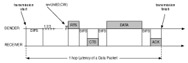
802.11 RTS/CTS: with the RTS/CTS DCF the transmission of data between a sender and a receiver is regulated by means of a double handshaking scheme which employs three small-sized, control-packets to regulate the transmission of (larger) data packets (Figure 1). The sender senses the channel for a randomly chosen duration before sending a RTS control packet to the receiver, on reception of which, the receiver, replies with a CTS control packet to the sender (first handshaking). The actual transmission of DATA packets starts as soon as the sender has received the CTS. Finally when the DATA transmission is over, the receiver acknowledges the sender with an ACK control packet (second handshaking). The RTS-CTS-DATA-ACK timing sequence is illustrated in Figure 1, which also points out the latency for a successful transmission of a DATA packet over 1-hop. To decrease the probability of collisions, the carrier-sensing time $t_{CS}$, also named Contention Window (CW), which is discretely slotted in a finite number of slots of fixed duration $aSlot_{t}$ ($aSlot_{t}$ being a parameter of the standard whose value depends on the underlying PHY layer), is randomly chosen. A contention takes place when at least two stations are performing carrier-sensing at the same time. The one that has (randomly) chosen the shortest number of available slots in the CW, wins the contention. The loser, instead, goes into backoff and increases the dimension of the CW by a power of $2$ (i.e. the new contention window size $CW^{\prime}$ is given by $CW^{\prime}=(CW_{m}+1)\cdot 2^{bc}-1$ where $bc$, the BackoffCounter, increases with the number of consecutive unsuccessful transmissions). The minimum and maximum size of contention window, respectively $CW_{m}$ and $CW_{M}$, are set by the standard and depends on the PHY layer. For the Frequency Hopping Single Spectrum (FHSS) PHY layer they are equal to $CW_{min}\!=\!16$ (initial value of $bc=0$) and $CW_{max}\!=\!1024$ (maximum value of $bc_{max}=6$). Apart from $t_{CS}$, two fixed-length time intervals are also relevant in the RTS/CTS DCF, namely: Distributed InterFrame Space (DIFS), the Short InterFrame Space (SIFS), where $SIFS\!<\!DIFS$ and which are defined by the PHY layer in the adopted networking stack (see Table 1). It should be noted that a collision can take place not only when two contending stations (randomly) pick the same carrier-sensing time (i.e. $t_{CS}$), but also, as pointed out by Heindl it et al. [10], because of the existence of the so-called vulnerable period, which accounts for three factors: the time of radio waves propagation through the medium ($aAirPropagationTime$), the time a station takes for accessing the medium ($aCCATime$) and the time a station takes for switching from receiving to transmitting mode($aRxTxTurnaroundTime$). As a consequence the duration of $aSlot_{t}$ is set by the IEEE standard to a value larger than the vulnerable period (i.e. the value $aSlot_{t}$ depends on the PHY-layer dependent parameters $aCCATime$ and $aRxTxTurnaroundTime$ plus the negligible $aAirPropagationTime$).

802.11p RTS/CTS with priority classes: The 802.11p MAC is based on an extension of the CSMA/CA RTS/CTS scheme, called Enhanced Distributed Channel Access (ECDA), which supports 4 priority levels, called Access Categories (AC), for data traffic, namely: Background (AC_BK), i.e. the lowest priority, Best effort (AC_BE), Video (AC_VI) and Voice (AC_VO), i.e. the highest priority. EDCA is designed so that higher-priority traffic is more likely (than lower-priority) to be be granted access to the shared medium and successfully being transmitted. In practice this is obtained by associating each AC with a contention window (CW) whose size is inversely proportional to the corresponding priority level. Therefore, for example, the CW for AC_BK (lowest priority) has to be larger than that of AC_VO (highest priority). Table 2 depicts the CW characterisation for the ACs of ECDA, where aCWmin and aCWmax are parameters set by the 802.11p protocol. One can notice that AC_VO is the dominant AC as its CW is not only the minimal one but also it does not overlap to the CW of any other AC.

3 Background: stochastic symmetric Petri nets

To carry out the performance modelling study of 802.11 protocols we used a coloured stochastic Petri net formalism, namely the Stochastic Symmetric Net (SSN) [8], to model networks using 802.11/802.11p MAC, and we applied the Hybrid Automata Specification Language (HASL) [5] formalism (through the C OSMOS  statistical model checker [4]) to assess relevant performance indicators against the SSN models. For the sake of space we only give a very succinct overview of the SSN and HASL formalisms referring the reader to the literature for a detailed treatment.

Stochastic Symmetric Nets. Like any Petri net formalism an SSN model is a bi-partite graph consisting of place nodes (circles) and transition nodes (bars). Places may contain (countably many) tokens and are connected to transitions through arcs which are labelled with arc functions. An SSN model describes a continuous-time, discrete-state stochastic process whose states correspond with the possible markings of the SSN (a marking gives the content of each place of the SSN). The peculiarity of SSN models is that tokens may be associated with information, hence they may have different colours, instead of being all indistinguishable as with non-coloured PN formalisms. Therefore places and transitions of an SSN are associated with a color domain (CD) built from elementary types called color classes ($\{C1,...,Cn\}$) with $cd(p)$, resp. $cd(t)$, denoting the CD of place $p$, resp. transition $t$ (see Table 4 and Table 3 for the CDs of 802.11p SSN model). SSN color classes are finite, non empty and disjoint sets, they may be ordered (in this case a successor function is defined on the class, inducing a circular order among the elements in the class), and may be partitioned into (static) subclasses. An SSN transition may be immediate (drawn as a thin filled in bar) or timed which means its firing delay is sampled (the moment it gets enabled) from a probability distribution that may be exponential (thick empty bar) or general (thick filled in bar). A coloured transition may be associated with a guard, i.e. a boolean-valued expression built on top of colored variables by means of the following basic predicates: $x\!=\!y$, $x\!\in\!\mathit{subclass}$, $d(x)\!=\!d(y)$ where $x$ and $y$ are variables of the transition with same type, and $d(x)$ denotes the static subclass $x$ belongs to.A valid transition binding is an assignment of values to its variables, satisfying the predicate expressed by the guard. A pair (transition,binding) is called transition instance. Each arc connecting a place $p$ and a transition $t$ is labeled with an expression denoting a function $\mathit{arcf:cd(t)\to Bag(cd(p))}$ where $Bag(A)$ is the set of all possible multisets that may be built on set $A$. The valuation of $\mathit{arcf}$ given a legal binding of $t$ gives the multiset of colored tokens to be withdrawn from (in case of input arc) or to be added to (in case of output arc) the place connected to that arc upon firing of such transition instance. The arc expressions in SSNs are built upon a limited set of primitive functions whose domains must be color classes. Typically an arc expression is a linear combination of function tuples (denoted $\langle f1,\ldots,fn\rangle$), and each element of a tuple is either a projection function, denoted by a variable in the transition color domain (e.g. $sa$ and $sb$ in the tuple $\langle sa,sb,p,pt\rangle$ appearing as the labelling in several arcs of the SSN of Figure 2), a successor function, denoted $\mathit{x\!+\!+}$ were $x$ is a variable whose type is an ordered class; a constant function, denoted $\mathit{C_{i}.All}$ returning all elements of (sub)class $C_{i}$; a complement function denoted $\mathit{C_{i}.All}\!-\!x$ where $x$ is a variable of type $C_{i}$. The dynamics of an SSN model is defined in terms of transition instances enabling and firing: a transition instance is enabled if the marking of all of its input places is compatible with it (i.e. if the marking enables the transition instance). Upon firing a transition instance modifies the state of the SSN by removing (resp. adding) tokens from its input (resp. output) places. For example, w.r.t. the SSN in Figure 2, assuming colour classes $\mathit{St\!=\!\{st1,st2\}}$ and $\mathit{Pr\!=\!\{pr1\}}$, the initial marking of place $\mathit{Idle}$ (colour domain $\mathit{St\!\times\!Pr}$) being $\mathit{\langle St,Pr\rangle\!=\!\{\langle st1,pr1\rangle,\langle st2,pr1\rangle\}}$ enables two instances of timed transition $\mathit{PacketArrival}$ (given its guard $sa\!\neq\!sb$), namely $\mathit{\langle st1,st2,pr1,rts\rangle}$ $\mathit{\langle st2,st1,pr1,rts\rangle}$. The firing of the first instance consumes $\mathit{\langle st1,pr1\rangle}$ from $\mathit{Idle}$ and adds $\mathit{\langle st1,st2,pr1,rts\rangle}$ to $\mathit{Sense}$.

4 Modelling of 802.11/802.11p networks

To analyse the performance of two versions of the protocol we developed two SSN models, one modelling a network whose stations use the 802.11 MAC, the other where stations that use the 802.11p MAC. The models we developed are based on the following assumptions: 1) Clicque network topology: the network consists of $N$ stations arranged in a clique (i.e. every station can overhear every other station). 2) Traffic direction: each station has a unique target station to which it addresses its incoming traffic. 3) Incoming traffic: each station is either under a) a saturated regime (i.e. a packet ready to be transmitted is invariably present) or b) its incoming traffic is given by an Poisson process with parameter $\lambda$. 4) Perfect/Imperfect channel: the wireless medium is supposed to behave either a) as a perfect channel (i.e. transmitted data are never affected by errors) or b) as an imperfect channel with some error probability (details below). 5) Vulnerable period: the radio device of each station is supposed to exhibit a certain delay for switching between transmission/reception mode. The duration of such period is called the vulnerable period and is one source of traffic collisions within the network.
Channel error model. To model the possibility that transmissions undergo errors due to the channel we adopted the burst-noise binary channel model [9]. A burst noise channels may be subsumed by a two-states Markov chain where one state ($G$ as in good) represents the absence of noise while the other ($B$ as in burst errors) represents the presence of an error spike which affects the channel impeding a transmission to correctly take place. We equipped our Petri nets models with an implementation of such burst-noise binary channel model.

4.1 SSN models of 802.11/802.11p networks

We developed two SSN models one for 802.11 networks the other for 802.11p’s. For the sake of space we only present the 802.11p version of the model, which is somehow a generalisation of the 802.11’s. The 802.11p SSN model relies on the definition of a number of color classes (Table 3) and color domains (Table 4) that are used to characterise the type of the various elements (places and tranisitions). The model consists essentially of three parts: the 802.11p core module, representing the prioritised carrier-sensing and RTS/CTS handshaking mechanism, the backoff module, representing the behaviour of a station in case of a collision and the medium module representing the state of the wireless channel. We present these 3 modules separately bearing in mind that they are part of the same SSN model.

Figure 2: SSN model of the 802.11p prioritised RTS/CTS scheme

802.11p core SSN module

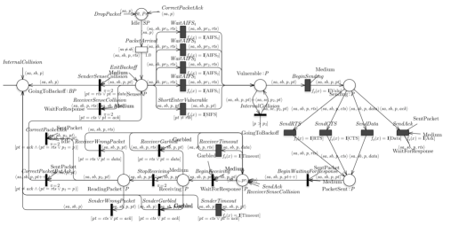
Figure 2 depicts the portion of the SSN model representing the traffic generation and prioritised RTS/CTS handshaking protocol. It consists of three main parts: the generation of incoming data traffic (timed transition $\mathit{PacketArrival}$), the carrier-sensing phase (timed transitions $\mathit{WaitAIFS}_{i}$, $\mathit{WaitSIFS}$), the packets transmission phase (timed transitions $\mathit{sendRTS}$, $\mathit{sendCTS}$, $\mathit{sendDATA}$, $\mathit{sendACK}$), the handling of packets received/overheard by a station (the sub-net in between places $\mathit{WaitForResponse}$, $\mathit{Receiving}$ and $\mathit{ReadingPacket}$). Let us describe the various parts of the model. Place $\mathit{Idle}$ (color domain $\mathit{SP}$) is initially filled up with tokens corresponding with all pairs from $\mathit{St}\!\times\!\mathit{Pr}$, representing that each station may generate incoming traffic with any level of priority. The firing of the outgoing timed (exponentially distributed) transition $\mathit{PacketArrival}$ consumes a $\langle sa,p\rangle$ token and produces the $\langle sa,sb,p,rts\rangle$ token (added to place $\mathit{Sense}$) indicating that station $sa$ is ready to send an $rts$ request with priority $p$ to station $sb$ ($sa\!\neq\!sb$). A token $\langle sa,sb,p,pt\rangle$ in place $\mathit{Sense}$ (representing an ongoing transmission of a packet of type $pt$ and priority $p$ from station $sa$ to $sb$) is then moved either to i) place $\mathit{Vulnerable}$ through either one of the four mutually-exclusive timed (deterministic) transition $\mathit{WaitAIFS}_{i}$ (only that corresponding to the actual priority value $p$ is enabled), if packet type $pt\!=\!rts$ and the medium remains free for $\mathit{AIFS}_{i}$ time units, or through $\mathit{WaitSIFS}$ if packet type $pt\!\neq\!rts$ and medium stay free for $\mathit{SIFS}$, or if the medium gets occupied in the meantime ii) to $\mathit{GoingToBackoff}$ (through immediate transition $\mathit{SenderSenseCollision}$) if $sa$ is the sender of an $rts$ or $data$ packet or iii) to $\mathit{WaitForResponse}$ (through immediate transition $\mathit{ReceiverSenseCollision}$) if $sa$ is a station responding with either a $cts$ or $ack$ to $sb$. A token $\langle sa,sb,p,pt\rangle$ from place $\mathit{Vulnerable}$ moves to $\mathit{Sending}$ (after $\mathit{Vuln}$ time units through timed transition $\mathit{BeingSending}$), and in so doing it adds one (uncoloured) token to $\mathit{Medium}$ indicating that the number of transmitting stations has increased. Observe that the immediate transition $\mathit{InternalCollision}$ (which is also consuming tokens from $\mathit{Vulnearble}$) deals with the case of competing packets sent, with different level of priorities, by a common station $sa$: in this case only the packet with the highest priority stays in $\mathit{Vulnerable}$, while packets with lower priority are moved to $\mathit{GoingToBackoff}$ (i.e. highest priority packet wins the internal competition by “overtaking” lower priority packets). From place $\mathit{Sending}$ a token $\langle sa,sb,p,pt\rangle$ moves to $\mathit{PacketSent}$ if the packet type is either $rts$, $cts$ or $data$, after a delay corresponding with the kind of packets, and then, with no delay, it is further moved to $\mathit{WaitForResponse}$ through immediate transition $\mathit{BeginWaitingForResponse}$ which while removing a token from $\mathit{Medium}$ (hence decreasing the occupation of the wireless channel) and storing the $\langle sa,sb,p,pt\rangle$ in place $\mathit{SentPacket}$ for later retrieval, also updates the packet type of token $\langle sa,sb,p,pt\rangle$ to $\langle sa,sb,p,pt\!+\!+\rangle$, indicating that station $sa$ is now ready to wait for a reply message (of type $pt\!+\!+$, i.e. $cts$ in reply to $rts$ or $ack$ in replay to $data$) from $sb$. Place $\mathit{WaitForResponse}$ is initialised with marking $\langle St,s1,pr1,rts\rangle$ indicating that each station of $St$ is, initially, ready to get engaged into replying to an $rts$ request ($s1$ and $pr1$ being irrelevant at this stage). As the medium gets occupied but not garbled all tokens in $\mathit{WaitForResponse}$ are moved (with no delay) to $\mathit{Receiving}$ and from there, as soon as the channel gets free (and assuming it hasn’t been garbled before) they move on to $\mathit{ReadingPacket}$. Thus, at the end of a transmission phase, place $\mathit{ReadingPacket}$ contains all tokens representing all possible combinations of responses that all stations may be engaged in. On completion of the transmission corresponding to token $\langle sb,sa,p,pt\rangle$ being added to $\mathit{SentPacket}$ the corresponding token $\langle sa,sb,p_{2},pt\rangle$, if present, is consumed from $\mathit{ReadingPacket}$ (through either one of the prioritised transitions $\mathit{CorrectPacketButAck}$ or $\mathit{CorrectPacketAck}$) representing the creation of the response, by the destination station $sa$, to the transmitted packet $pt$. Notice that $\mathit{CorrectPacketButAck}$ triggers the response to an $\mathit{rts}$, $\mathit{cts}$ or $\mathit{data}$ packet by adding the token $\langle sa,sb,p,pt\!+\!+\rangle$ to $\mathit{Sense}$ hence moving to the next step of the RTS/CTS protocol for the processed packet. Conversely $\mathit{CorrectPacketAck}$ represents the end of the RTS/CTS handshaking hence it puts back a $\langle sa,p\rangle$ token to $\mathit{Idle}$ which restart the cycle for the transmission of a priority level $p$ packet by station $sa$. On the other hand all tokens $\langle sa,sb,p,pt\rangle$ that remain in $\mathit{ReadingPacket}$ after a response to the transmitted packet has been treated (through either $\mathit{CorrectPacketButAck}$ or $\mathit{CorrectPacketAck}$) are either put back to $\mathit{WaitForResponse}$ (if they represent a receiver, i.e. transition $\mathit{ReceiverWrongPacket}$) or they are moved to $\mathit{GoingToBackoff}$ (if they represent a sender that was expecting either a $\mathit{cts}$ or an $\mathit{ack}$ response to a previosuly sent packet $\mathit{rts}$ or $\mathit{data}$).

Figure 3: SSN model of the 802.11p backoff mechanism (top left) and the medium (bottom right).

802.11p backoff SSN module

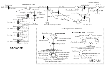
With the 802.11p DCF the selection of the backoff duration, i.e. the selection of the number of time slots a packet has to wait before starting a new transmission attempt, depends on the priority class of the packet as well as on the backoff round, i.e. the number of times a packet has unsuccessfully went through the carrier-sensing phase without winning the contention. Therefore a model of 802.11p backoff procedure must be equipped with necessary means to take into account the priority level of each packet hence the size of the contention window for each priority level. Figure 3 (top left) depicts the SSN subnet representing the randomised selection of the backoff delay for a packet of a given priority level $p$. A backoff begins when a token $\langle sa,sb,p\rangle$ is added to place $\mathit{GoingToBackoff}$ (color domain $\mathit{BP}$) indicating that something went wrong (e.g. a collision or a lack of handshaking) during the transmission of a priority $\mathit{p}$ packet from station $\mathit{sa}$ towards $\mathit{sb}$. The first step then is the updating of the backoff round counter which boils down to adding of a token $\langle sa,sb,p,tx\rangle$ to place $\mathit{TxAttemptsCounter}$ (whose color domain is $\mathit{SRPCoun}t$ and where variable $\mathit{tx}\!\in\!\mathit{TxCount}$ stores the backoff counter) through either transition $\mathit{GoToBackoff}$ (enabled if the failed transmission attempt is the first one, hence initialising $\mathit{tx}$ to color $\mathit{tx_{1}}$) or through transition $\mathit{ReturnToBackoff}$ (enabled by any further failed transmission attempt and increasing $\mathit{tx}$ by 1). Once a token $\langle sa,sb,p\rangle$ enters place $\mathit{ChoosingBackoff}$ having, in the process, also added (or updated) a $\langle sa,sb,p,tx\rangle$ token to place $\mathit{TxAttemptsCounter}$, either one between the mutually exclusive transitions $\mathit{ChooseBackoff}$ or $\mathit{DropPacket}$ transition is enabled. Transition $\mathit{ChooseBackoff}$ realises the probabilistic selection of the backoff counter value $b$, corresponding to the priority level $p$ of the backoffing packet, by adding token $\langle sa,sb,p,b\rangle$ to place $\mathit{BackoffCounter}$. Such a selection is achieved through randomly choosing (through the test arc between transition $\mathit{ChooseBackoff}$ and place $\mathit{BackoffMappings}$) a token $\langle p,tx,b\rangle$ among those specified by the invariant marking of $\mathit{BackoffMappings}$ (Table 5). The marking of $\mathit{BackoffMappings}$ associates with each priority level $\mathit{pr_{i}}$ and re-transmission attempt $\mathit{tx_{j}}$ the corresponding CW expressed as the union of color subclasses $\cup_{k=1}^{k^{\prime}}bs_{k}$ (where $k^{\prime}$ is a function of $pr_{i}$ and $tx_{j}$). Therefore, for example, for the first re-transmission attempt (i.e. $\mathit{tx=tx_{1}}$) of a priority $p_{1}$ packet the backoff value $b$ is chosen randomly as $b\in\ \mathit{bs_{1}}=\mathit{\{b1,\ldots,b4\}}$ (which corresponds with the narrowest CW i.e. the AC_V0 category) as the initial marking $\mathit{BM_{0}}$ contains tokens $<pr1,tx1,bs1>$. Similarly for the second re-transmission attempt (of a priority $p_{1}$ packet) $b$ is chosen randomly as $b\in\ \mathit{bs_{1}}\cup\mathit{bs_{2}}=\mathit{\{b1,\ldots,b8\}}$ as marking $\mathit{BM_{0}}$ contains tokens $<pr1,tx2,bs1+bs2>$ and so on. Once a $\langle sa,sb,p,b\rangle$ token is added to place $\mathit{BackoffCounter}$ (i.e. the backoff delay $b$ is selected) the actual backoff (sensing) period begins: $b$ is decremented every $\mathit{aSlot}$ time units (deterministic transition $\mathit{DecrementBackoff}$) however, as soon as the medium gets occupied, the decrement of $b$ is suspended by moving token $\langle sa,sb,p,b\rangle$ from $\mathit{BackoffCounter}$ to $\mathit{PausingBackoff}$ (immediate transition $\mathit{PauseBackoff}$). Token $\langle sa,sb,p,b\rangle$ is moved back to $\mathit{BackoffCounter}$ only after the channel got freed and stayed free for $\mathit{AIFS_{i}}$ time units (where $i\!\in\!\{1,2,3,4\}$ denotes the priority level $p$ of the backoff-ing packet). The backoff for a token $\langle sa,sb,p,b\rangle$ ends as soon as the backoff counter has reached 1 (i.e. $b\!=\!b1$): at this point token $\langle sa,sb,p,b1\rangle$ is removed from $\mathit{BackoffCounter}$ (immediate transition $\mathit{ExitBackoff}$) and $\langle sa,sb,p,rts\rangle$ is pushed back to $\mathit{Sense}$ which represent the re-start of the transmission procedure for station $\mathit{sa}$ to sent a priority $p$ packet to $\mathit{sb}$.

802.11p medium SSN module

Figure 3 (bottom right) shows the part of the SSN model representing the shared channel. It consists of 2 uncoloured places: $\mathit{Medium}$, whose marking corresponds with the number of transmitting stations, and $\mathit{Garbled}$, which contains a token whenever a collision has taken place or an error spike has occurred on the channel. Transition $\mathit{GettingGarbled}$ sets the state of the medium to garbled (adding a token in place $\mathit{Garbled}$) as soon as $\mathit{Medium}$ contains at least 2 tokens (i.e. at least two stations are transmitting). Transition $\mathit{EndingGarbled}$ ends the garbled state of the medium by removing a token from $\mathit{Garbled}$ as soon as the $\mathit{Medium}$ is emptied. Place $\mathit{SentPacket}$ (domain $P$) stores the information relative to an ongoing transmission in terms of a token $\mathit{\langle sa,sb,p,pt\rangle}$ where $sa$ is the sender station, $sb$ the receiver ,$p$ the priority level $p$ and $tp$ the packet type). The medium SSN is also equipped with a subnet for modelling the presence of error spikes affecting an ongoing transmission. To study the effect of a noisy channel on the network performances it suffices that place $\mathit{NotErrorSpike}$ initially contains a token in which case transition $\mathit{EnterinErrorSpike}$ reproduce the occurence of errors on the channel (following an Exponential distribution with configurable rate, $0.01$ in the picture), by adding a token in $\mathit{Medium}$ (hence triggering a collision if a transmission is going on). The end of an error-spike is modelled by transition $\mathit{ExitingErrorSpike}$ (also Exponentially distributed with a configurable rate).

5 analysis of 802.11/802p models

We analysed the performances of both the 802.11 and 802.11p network models  by means of the C OSMOS  statistical model checker [4, 1]. We considered a number of key performance indicators (KPI) including 1) the throughput (THR) of a network station (i.e. the number of successfully transmitted packets per time unit); 2) the busyTimeRatio (BTR, i.e. the ratio between the time the channel is occupied by some transmitting station and the total operation time of the network). We encoded such KPIs in terms of HASL specifications for SSN models [3] and used them to run a number of experiments to assess the impact that 1) a faulty channel, 2) the incoming traffic, 3) the network dimension have on the KPIs. In the remainder we present an excerpt of the results obtained. Figure 4 shows an example of an HASL specification (a linear hybrid automaton, LHA) we used to assess the THR for priority $p$ traffic on the 802.11p model.

[scale=.6]./sectionsCR/lha1

Figure 4: The LHA for measuring the throughput

The LHA in Figure 4 has an initial ($l_{1}$) and a final ($l_{2}$) location and uses a clock ($t$) plus a counter of successfully terminated transmissions for a priority $p$ packet ($Throughput[p]$). On processing a trajectory $Throughput[p]$ is incremented each time an instance of the $\mathit{CorrectButAck}$ transition (Figure 2) with the corresponding priority $p$ level occur (which coincides with the termination of the transmission of a priority $p$ packet). The LHA ends measure at time $T$ and the value of THR is obtained as $Throughput[p]/T$.

(a) Throughput 802.11

(b) BusyTimeRatio 802.11

(c) saturated traffic 802.11

(d) 2 stations, non-saturated traffic 802.11

(e) Throughput 802.11p

(f) BusyTimeRatio 802.11p

(g) traffic rate $\lambda\!=\!100$ 802.11p

(h) traffic rate $\lambda\!=\!1000$ 802.11p

Figure 5: Impact of network dimension and noisy-channel on throughput and BTR for 802.11 and 802.11p networks

5.1 Results

Impact of network dimension and incoming traffic.

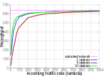
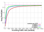
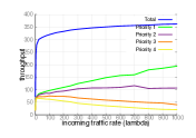
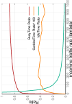
Figure 5(a) and 5(b) depict the estimated THR and BTR for the 802.11 model computed (for different network dimensions) in function of the traffic arrival rate $\lambda$ (i.e. under a non-saturated regime) and assuming the channel is not affected by errors (ideal channel). Both the THR and the BTR exhibit an asymptotic profile (the faster the inter-arrival rate the higher the throughput, resp. the BTR) and both are upper bounded by the nominal maximum throughput under saturated regime (which is $\sim\!640$ packets per second), resp. the saturated nominal maximum BTR Figure 5(e) and 5(f), refer to the same kind of experiment for the 802.11p model (for a network with $N=2$ nodes). Plots in Figure 5(e) highlight the effect of prioritised management of data traffic: the higher the traffic the larger the difference between high priority and low priority throughput. Figure 5(f) shows the BTR as well as the ratio between the time the channel is idle (over the total observation time) and the ratio between the time the channel is garbled (collision).

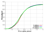
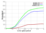
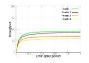
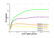
Impact of faulty channel. Figure 5(c),  5(d),  5(g) and 5(h) report on assessing the effect that a faulty channel has on the network performances. The THR and BTR are measured in function of the period of an error spike (determined by the rate of transition $\mathit{EnteringErrorSpike}$). Results show that the throughput increases with the error-spike period however (for the 802.11 model under saturated regime Figure 5(c)) the THR is unaffected by the network dimension (identical plot for different number of stations) indicating that the performances gradient induced by the network dimension in case of ideal channel (Figure 5(a)) fades away in presence of a faulty channel. Conversely under a non-saturated regime (802.11 model Figure 5(d)) the error-spike period affects the throughput differently depending on the traffic arrival rates. Finally Figure 5(g) and 5(h) show the effect of the error-spike on the prioritised throughput in a 802.11p network showing that the effect of a faulty channel, in terms of the gradient between higher and lower priority throughput is more evident under a high traffic regime (Figure 5(h)) than under a low traffic regime (Figure 5(g)).

6 Conclusion

We presented a performance modelling study of two versions of MAC protocol for wireless networks: the 802.11 MAC and its prioritised extension 802.11p devoted to VANETS. We developed our models using a high-level stochastic Petri nets formalism which allowed us to encode the complexity of the 802.11 prioritised scheme in a model of reasonable size. The models we presented are highly configurable and allow for the analysis of the performance of networks in different respect (traffic conditions, ideal or imperfect channel, network dimension). We analysed the performance on the network models by means of statistical model checking based on the HASL specification language. Future work include the extension of the models to $N$-hops topologies, which would allow us to take into account the effect of routing on the performances of a given network.

7 Parameters of the SSN model of the 802.11 and 802.11p MAC

name	meaning	value ($\times\!10\mu s$)
aslot	the time unit of the backoff procedure	2
nStations	# of stations	2
packetSizeInAslot	# of time slot for sending a DATA packet	variable
DIFS	the length of the DCF interframe space	5
SIFS	the length of a short interframe space	1
vuln	delay to switch radio from RX-to-TX mode	2
RTS	the time it takes to send a RTS packet	16
CTS	the time it takes to send a CTS packet	11
ACK	the time it takes to send an aknowledgement packet	11
timeout	delay a station waits for handshaking packet	5
CWmin	min. size of the contention window (in aslot)	15
backoffMax	# of TX attempts before dropping a packet	6
deadline	# of time slots for entering the livelock (end) state	5000

Table 1: Timing parameters for the SSN models of RTS/CTS

AC	CWmin	CWmax
Background (AC_BK)	aCWmin	aCWmax
Best effort (AC_BE)	aCWmin	aCWmax
Video (AC_VI)	[(aCWmin+1)/2]-1	aCWmin
Voice (AC_VO)	[(aCWmin+1)/4]-1	[(aCWmin+1)/2]-1

Table 2: Contention windows boundaries for ECDA access categories.

name	description	definition	ordered
$PT$	Packet Type	$PT\!=\!\{rts,cts,data,ack\}$	YES
$St$	Station ID	$St\!=\!s\{1,\ldots,N\}$	NO
$Pr$	Priority level (of a packet)	$Pr\!=\!p\{1,\ldots,4\}$	NO
$TxCount$	max. num. of re-transmissions before dropping a packet	$TxCount\!=\!tx\{1,\ldots,20\}$	YES
$\mathit{BackoffStage}$	backoff counter domain	$\mathit{BackoffStage}\!=\!bs_{1}\cup\ldots\cup bs_{9}$	YES
$bs_{1}$	backoff counter domain stage 1	$bs_{1}\!=\!b\{1,\ldots,4\}$	YES
$bs_{2}$	backoff counter domain stage 2	$bs_{2}\!=\!b\{5,\ldots,8\}$	YES
$bs_{3}$	backoff counter domain stage 3	$bs_{3}\!=\!b\{9,\ldots,16\}$	YES
$bs_{4}$	backoff counter domain stage 4	$bs_{4}\!=\!b\{17,\ldots,32\}$	YES
$bs_{5}$	backoff counter domain stage 5	$bs_{5}\!=\!b\{33,\ldots,64\}$	YES
$bs_{6}$	backoff counter domain stage 6	$bs_{6}\!=\!b\{65,\ldots,128\}$	YES
$bs_{7}$	backoff counter domain stage 7	$bs_{7}\!=\!b\{129,\ldots,256\}$	YES
$bs_{8}$	backoff counter domain stage 8	$bs_{8}\!=\!b\{257,\ldots,512\}$	YES
$bs_{9}$	backoff counter domain stage 9	$bs_{9}\!=\!b\{513,\ldots,1024\}$	YES

Table 3: Color classes for the SSN model of the 802.11p protocol.

name	description	definition
$SR$	Sender-Receiver	$SR\!=\!St\times St$
$SP$	Station-Priority	$SP\!=\!St\times Pr$
$BP$	Backoff-Priority	$BP\!=\!St\times St\times Pr$
$P$	Packet sending	$P\!=\!St\times St\times Pr\times PT$
$SRB$	Sender-Receiver-BackoffStage	$SRB\!=\!St\times St\times\mathit{BackoffStage}$
$BPMap$	Mapping-Priority-Backoff	$BPMap\!=\!Pr\times TxCount\times\mathit{BackoffStage}$
$SRPcount$	Sender-Recevier-Priority-Count	$SRPcount\!=\!St\times St\times Pr\times\mathit{TxCount}$

Table 4: Color domains for the SSN model of the 802.11p protocol.

marking

definition

$\mathit{BM_{0}}$

<pr1,tx1,bs1>+<pr1,tx2,bs1+bs2>+<pr1,tx3,bs1+bs2>+<pr1,tx4,bs1+bs2> +<pr2,tx1,bs1>+<pr2,tx2,bs1+bs2>+<pr2,tx3,bs1+bs2+bs3> + +<pr2,tx4,bs1+bs2+bs3>+<pr2,tx5,bs1+bs2+bs3>+<pr3,tx1,bs1+bs2> + <pr3,tx2,bs1+bs2+bs3>+<pr3,tx3,bs1+bs2+bs3+bs4> +<pr3,tx4,bs1+bs2+bs3+bs4+bs5> + <pr3,tx5,bs1+bs2+bs3+bs4+bs5+bs6> +<pr3,tx6,bs1+bs2+bs3+bs4+bs5+bs6+bs7> + <pr3,tx7,bs1+bs2+bs3+bs4+bs5+bs6+bs7+bs8> +<pr3,tx8,bs1+bs2+bs3+bs4+bs5+bs6+bs7+bs8+bs9> + <pr3,tx9,bs1+bs2+bs3+bs4+bs5+bs6+bs7+bs8+bs9> + <pr3,tx10,bs1+bs2+bs3+bs4+bs5+bs6+bs7+bs8+bs9> +<pr4,tx1,bs1+bs2+bs3>+<pr4,tx2,bs1+bs2+bs3+bs4> +<pr4,tx3,bs1+bs2+bs3+bs4+bs5>+<pr4,tx4,bs1+bs2+bs3+bs4+bs5+bs6> +<pr4,tx5,bs1+bs2+bs3+bs4+bs5+bs6+bs7> +<pr4,tx6,bs1+bs2+bs3+bs4+bs5+bs6+bs7+bs8> +<pr4,tx7,bs1+bs2+bs3+bs4+bs5+bs6+bs7+bs8+bs9> + <pr4,tx8,bs1+bs2+bs3+bs4+bs5+bs6+bs7+bs8+bs9> + <pr4,tx9,bs1+bs2+bs3+bs4+bs5+bs6+bs7+bs8+bs9>

Table 5: Invariant marking of place $\mathit{BackoffMapping}$.

References

- [1] Cosmos home page. http://cosmos.lacl.fr.
- [2] Ahed Alshanyour and Anjali Agarwal. Performance of IEEE 802.11 RTS/CTS with finite buffer and load in imperfect channels: Modeling and analysis. In Proceedings of the Global Communications Conference, 2010. GLOBECOM 2010, 6-10 December 2010, Miami, Florida, USA, pages 1–6. IEEE, 2010.
- [3] Elvio Gilberto Amparore, Benoit Barbot, Marco Beccuti, Susanna Donatelli, and Giuliana Franceschinis. Simulation-based verification of hybrid automata stochastic logic formulas for stochastic symmetric nets. In Proceedings of the 1st ACM SIGSIM Conference on Principles of Advanced Discrete Simulation, SIGSIM PADS ’13, pages 253–264, New York, NY, USA, 2013. ACM.
- [4] P. Ballarini, H. Djafri, M. Duflot, S. Haddad, and N. Pekergin. COSMOS: A statistical model checker for the hybrid automata stochastic logic. In Proceedings of the 8th International Conference on Quantitative Evaluation of Systems (QEST’11), pages 143–144. IEEE Computer Society Press, sep. 2011.
- [5] Paolo Ballarini, Benoît Barbot, Marie Duflot, Serge Haddad, and Nihal Pekergin. Hasl: A new approach for performance evaluation and model checking from concepts to experimentation. Performance Evaluation, 90:53 – 77, 2015.
- [6] Frederico J. R. Barboza, Aline Maria Santos Andrade, Flávio Morais de Assis Silva, and George Lima. Specification and verification of the IEEE 802.11 medium access control and an analysis of its applicability to real-time systems. Electr. Notes Theor. Comput. Sci., 195:3–20, 2008.
- [7] G. Bianchi. Performance analysis of the IEEE 802.11 distributed coordination function. IEEE J.Sel. A. Commun., 18(3):535–547, September 2006.
- [8] G. Chiola, C. Dutheillet, G. Franceschinis, and S. Haddad. Stochastic well-formed colored nets and symmetric modeling applications. IEEE Trans. Comput., 42(11):1343–1360, November 1993.
- [9] E. N. Gilbert. Capacity of a burst-noise channel. Bell System Technical Journal, 39:1253–1265, 1960.
- [10] Armin Heindl and Reinhard German. Performance modeling of ieee 802.11 wireless lans with stochastic petri nets. Performance Evaluation, 44:139–164, 2000.
- [11] IEEE. The OSI reference model., 1983.
- [12] IEEE. Ieee wirless lan medium access control (mac) and physical layer(phy) specification std 802.11-1997. Technical report, Institute of Electrical and Electronic Engineers, 1997.
- [13] M. Kwiatkowska, G. Norman, and J. Sproston. Probabilistic model checking of the IEEE 802.11 wireless local area network protocol. In H. Hermanns and R. Segala, editors, Proc. 2nd Joint International Workshop on Process Algebra and Probabilistic Methods, Performance Modeling and Verification (PAPM/PROBMIV’02), volume 2399 of LNCS, pages 169–187. Springer, 2002.
- [14] A. Lyakhov and F. Simatos. Hybrid rts/cts mechanism in wi-fi ad hoc networks with correlated channel failures. 17th IMACS, 2015.