An asynchronous, forward-backward, distributed generalized Nash equilibrium seeking algorithm.

Abstract

In this paper, we propose an asynchronous distributed algorithm for the computation of generalized Nash equilibria in noncooperative games, where the players interact via an undirected communication graph. Specifically, we extend the paper “Asynchronous distributed algorithm for seeking generalized Nash equilibria” by Yi and Pavel: we redesign the asynchronous update rule using auxiliary variables over the nodes rather than over the edges. This key modification renders the algorithm scalable for highly interconnected games. The derived asynchronous algorithm is robust against delays in the communication and it eliminates the idle times between computations, hence modeling a more realistic interaction between players with different update frequencies. We address the problem from an operator-theoretic perspective and design the algorithm via a preconditioned forward-backward splitting. Finally, we numerically simulate the algorithm for the Cournot competition in networked markets.

I INTRODUCTION

I-A Motivation and literature overview

Noncooperative generalized games over networks is currently a very active research field, due to the spreading of multi-agent network systems in modern society. Such type of games emerge in several application domains, such as smart grids [1, 2], social networks [3] and robotics [4]. In a game setup the players, or agents, have a private and local objective function that depends on the decisions of some other players, which shall be minimized while satisfying both local and global, coupling, constraints. Typically each agent defines its decision, or strategy, based on some local information exchanged with a subset of other agents, called neighbors. One popular notion of solution for these games is a collective equilibrium where no player benefits from changing its strategy, e.g. a generalized Nash equilibrium (GNE). Various authors proposed solutions to this problem [5, 3, 6]. These works propose only synchronous solutions for solving noncooperative games. So, all the agents shall wait until the slowest one in the network completes its update, before starting a new operation. This can slow down the convergence drammatically, especially in large scale and heterogeneous systems. On the other hand, adopting an asynchronous update reduces the idle times, increasing efficiency. In addition, it can also speed up the convergence, facilitate the insertion of new agents in the network and even increse robusteness w.r.t. communication faults [7]. The pioneering work of Bertsekas and Tsitsiklis [8] can be considered the starting point of the literature on parallel asynchronous optimization. During the past years, several asynchronous algorithms for distributed convex optimization were proposed [9, 10, 11, 12], converging under different assumptions. The novel work in [13], provides a simple framework (ARock) to develop a wide range of iterative fixed point algorithms based on nonexpansive operators and it is already adopted in [14] to seek variational GNE seeking under equality constraints and using edge variables.

In this paper, we propose an extension of the work in [14]. Specifically, we consider inequality coupling constraints and use a restricted set of auxiliary variables, namely, associated with the nodes rather than with the edges. Especially this latter upgrade is non-trivial and presents technical challenges in the asynchronous implementation of the algorithm, which we overcome by analyzing the influence of the delayed information on the update of the auxiliary variables. The use of node variables only, rather than edge variables, preserves the scalability of the algorithm, with respect to the number of nodes.

I-B Structure of the paper

The paper is organized as follows: Section III formalizes the problem setup and introduces the concept of variational v-GNE. In Section IV the iterative algorithm for v-GNE seeking is derived for the synchronous case. The asynchronous counterpart of the algorithm is presented in Section V. Section VI is dedicated to the simulation results for the problem of Cournot competition in networked markets. Section VII ends the paper presenting the conclusions and the outlooks of this work.

II NOTATION

II-A Basic notation

The set of real, positive, and non-negative numbers are denoted by $\mathbb{R}$, $\mathbb{R}_{>0}$, $\mathbb{R}_{\geq 0}$, respectively; $\overline{\mathbb{R}}:=\mathbb{R}\cup\{\infty\}$. The set of natural numbers is $\mathbb{N}$. For a square matrix $A\in{\mathbb{R}}^{n\times n}$, its transpose is $A^{\top}$, $[A]_{i}$ is the $i$-th row of the matrix and $[A]_{ij}$ represents the elements in the row $i$ and column $j$. $A\succ 0$ ($A\succeq 0$) stands for positive definite (semidefinite) matrix, instead $>$ ($\geq$) describes element wise inequality. $A\otimes B$ is the Kronecker product of the matrices $A$ and $B$. The identity matrix is denoted by $I_{n}\in{\mathbb{R}}^{n\times n}$. $\boldsymbol{0}$ ($\boldsymbol{1}$) is the vector/matrix with only $0$ ($1$) elements. For $x_{1},\dots,x_{N}\in\mathbb{R}^{n}$, the collective vector is denoted as $\boldsymbol{x}:=\mathrm{col}(x_{1},\dots,x_{N})=[x_{1}^{\top},\dots,x_{N}^{\top}]^{\top}$. ${\mathrm{diag}}(A_{1},\dots,A_{N})$ describes a block-diagonal matrix with the matrices $A_{1},\dots,A_{N}$ on the main diagonal. The null space of a matrix $A$ is $\mathrm{ker}(A)$. The Cartesian product of the sets $\Omega_{i}$, $i=1,\dots,N$ is $\prod^{N}_{i=1}\Omega_{i}$.

II-B Operator-theoretic notation

The identity operator is by $\textrm{Id}(\cdot)$. The indicator function $\iota_{\mathcal{C}}:{\mathbb{R}}^{n}\rightarrow[0,+\infty]$ of $\mathcal{C}\subseteq{\mathbb{R}}^{n}$ is defined as $\iota_{\mathcal{C}}(x)=0$ if $x\in\mathcal{C}$; $+\infty$ otherwise. The set valued mapping $N_{\mathcal{C}}:{\mathbb{R}}^{n}\rightrightarrows{\mathbb{R}}^{n}$ denotes the normal cone to the set $\mathcal{C}\subseteq{\mathbb{R}}^{n}$, that is $N_{\mathcal{C}}(x)=\{u\in{\mathbb{R}}^{n}\,|\,\mathrm{sup}\langle\mathcal{C}-x,u\rangle\leq 0\}$ if $x\in\mathcal{C}$ and $\varnothing$ otherwise. The graph of a set valued mapping $\mathcal{A}:\mathcal{X}\rightrightarrows\mathcal{Y}$ is $\mathrm{gra}(\mathcal{A}):=\{(x,u)\in\mathcal{X}\times\mathcal{Y}\,|\,u\in\mathcal{A}(x)\}$. For a function $\phi:{\mathbb{R}}^{n}\rightarrow\overline{\mathbb{R}}$, define $\mathrm{dom}(\phi):=\{x\in{\mathbb{R}}^{n}|f(x)<+\infty\}$ and its subdifferential set-valued mapping, $\partial\phi:\mathrm{dom}(\phi)\rightrightarrows{\mathbb{R}}^{n}$, $\partial\phi(x):=\{u\in{\mathbb{R}}^{n}|\>\langle y-x|u\rangle+\phi(x)\leq\phi(y)\,,\>\forall y\in\mathrm{dom}(\phi)\}$. The projection operator over a closed set $S\subseteq{\mathbb{R}}^{n}$ is $\textrm{proj}_{S}(x):{\mathbb{R}}^{n}\rightarrow S$ and it is defined as $\textrm{proj}_{S}(x):=\mathrm{argmin}_{y\in S}\lVert y-x\rVert^{2}$. A set valued mapping $\mathcal{F}:{\mathbb{R}}^{n}\rightrightarrows{\mathbb{R}}^{n}$ is $\ell$-Lipschitz continuous with $\ell>0$, if $\lVert u-v\rVert\leq\ell\lVert x-y\rVert$ for all $(x,u)\,,\,(y,v)\in\mathrm{gra}(\mathcal{F})$; $\mathcal{F}$ is (strictly) monotone if $\forall(x,u),(y,v)\in\mathrm{gra}(\mathcal{F})$ $\langle u-v,x-y\rangle\geq(>)0$ holds true, and maximally monotone if it does not exist a monotone operator with a graph that strictly contains $\mathrm{gra}(\mathcal{F})$. Moreover, it is $\alpha$-strongly monotone if $\forall(x,u),(y,v)\in\mathrm{gra}(\mathcal{F})$ it holds $\langle x-y,u-v\rangle\geq\alpha\lVert x-y\rVert^{2}$. The operator $\mathcal{F}$ is $\eta$-averaged ($\eta$-AVG) with $\eta\in(0,1)$ if $\lVert\mathcal{F}(x)-\mathcal{F}(y)\rVert^{2}\leq\lVert x-y\rVert^{2}-\frac{1-\eta}{\eta}\lVert(\textrm{Id}-\mathcal{F})(x)-(\textrm{Id}-\mathcal{F})(y)\rVert^{2}$ for all $x,y\in{\mathbb{R}}^{n}$; $\mathcal{F}$ is $\beta$-cocoercive if $\beta\mathcal{F}$ is $\frac{1}{2}$-averaged, i.e. firmly nonexpansive (FNE). The resolvent of an operator $\mathcal{A}:{\mathbb{R}}^{n}\rightrightarrows{\mathbb{R}}^{n}$ is $\mathrm{J}_{\mathcal{A}}:=(\textrm{Id}+\mathcal{A})^{-1}$.

III Problem Formulation

III-A Mathematical formulation

We consider a set of $N$ agents (players), involved in a noncooperative game subject to coupling constraints. Each player $i\in\mathcal{N}:=\{1,\dots,N\}$ has a local decision variable (strategy) $x_{i}$ that belongs to its private decision set $\Omega_{i}\subseteq{\mathbb{R}}^{n_{i}}$, the vector of all the strategies played is $\boldsymbol{x}:=\mathrm{col}(x_{1},\dots,x_{N})\in{\mathbb{R}}^{n}$ where $n=\sum_{i\in\mathcal{N}}n_{i}$, and $\boldsymbol{x}_{-i}=\mathrm{col}(x_{1},\dots,x_{i-1},x_{i+1},\dots,x_{N})$ are the decision variables of all the players other than $i$. The aim of each agent $i$ is to minimize its local cost function $f_{i}(x_{i},\boldsymbol{x}_{-i}):\Omega_{i}\times\Omega_{-i}\rightarrow\overline{\mathbb{R}}$, where $\boldsymbol{\Omega}=\prod_{i\in\mathcal{N}}\Omega_{i}\subseteq{\mathbb{R}}^{n}$, that leads to a coupling between players, due to the dependency on both $x_{i}$ and the strategy of the other agents in the game. In this work we assume the presence of affine constraints between the agent strategies. These shape the collective feasible decision set

$$\mathcal{\boldsymbol{X}}:=\boldsymbol{\Omega}\cap\left\{\boldsymbol{x}\in{\mathbb{R}}^{n}\,|\,A\boldsymbol{x}\leq b\right\}\,,$$ (1)

where $A\in{\mathbb{R}}^{m\times n}$ and $b\in{\mathbb{R}}^{m}$. Then, the feasible set of each agent $i\in\mathcal{N}$ reads as

$$\mathcal{X}_{i}(\boldsymbol{x}_{-i}):=\left\{y\in\Omega_{i}\,|\,A_{i}y-b_{i}\leq\textstyle{\sum_{j\in\mathcal{N}\setminus\{i\}}}b_{j}-A_{j}x_{j}\right\}\,,$$

where $A=[A_{1},\dots,A_{N}]$, $A_{i}\in{\mathbb{R}}^{m\times n_{i}}$ and $\sum_{j=1}^{N}b_{j}=b$. We note that both the local decision set $\Omega_{i}$ and how the player $i$ is involved in the coupling constraints, i.e. $A_{i}$ and $b_{i}$, are private information, hence will not be accessible to other agents. Assuming affine constraints is common in the literature on noncooperative games [15, 5]. In the following, we introduce some other common assumptions over the aforementioned sets and cost function.

Standing Assumption 1 (Convex constraint sets)

For each player $i\in\mathcal{N}$, the set $\Omega_{i}$ is convex, nonempty and compact. The feasible local set $\mathcal{X}_{i}(\boldsymbol{x}_{-i})$ satisfies Slater’s constraint qualification. ∎

Standing Assumption 2 (Convex and diff. cost functions)

For all $i\in\mathcal{N}$, the cost function $f_{i}$ is continuous, $\beta$-Lipschitz continuous, continuously differentiable and convex in its first argument. ∎

In compact form, the game between players reads as

$$x_{i}\in\mathop{\mathrm{argmin}}\limits_{y\in{\mathbb{R}}^{n}}f_{i}(y,\boldsymbol{x}_{-i})\quad\textup{s.t.}\quad y\in\mathcal{X}_{i}(\boldsymbol{x}_{-i})\>.$$ (2)

In this paper, we are interested in the generalized Nash equilibia (GNE) of the game in (2).

Definition 1 (Generalized Nash equilibrium)

A collective strategy $\boldsymbol{x}^{*}$ is a GNE if, for each player $i$, it holds

$$x_{i}^{*}\in\mathop{\mathrm{argmin}}\limits_{y\in{\mathbb{R}}^{n}}f_{i}(y,\boldsymbol{x}_{-i}^{*})\quad\textup{s.t.}\quad y\in\mathcal{X}_{i}(\boldsymbol{x}_{-i}^{*})\>.$$ (3)

∎

III-B Variational GNE

Let us introduce an interesting subset of GNE, the set of so called variational GNE (v-GNE), or normalized equilibrium point, of the game in (2) referring to the fact that all players share a common penalty in order to meet the constraints. This is a refinement of the concept of GNE that has attracted a growing interest in recent years - see [16] and references therein. This set can be rephrased as solutions of a variational inequality (VI), as in [6].

First, we define the pseudo-gradient mapping of the game (2) as

$$F(\boldsymbol{x})=\mathrm{col}\left(\{\nabla_{x_{i}}f_{i}(x_{i},\boldsymbol{x}_{-i})\}_{i\in\mathcal{N}}\right)\,,$$ (4)

that gathers all the subdifferentials of the local cost functions of the agents. The following are some standard technical assumptions on $F$, see [17, 18].

Standing Assumption 3

The pseudo-gradient $F$ in (4) is $\ell$-Lipschitz continuous and $\alpha$-strongly monotone, for some $\ell,\alpha>0$. ∎

Standing Assumption 2 implies that $F$ is a single valued mapping, hence one can define VI($F,\boldsymbol{X}$) as the problem:

$$\textup{find }\boldsymbol{x}^{*}\in\boldsymbol{X},\>\textup{s.t.}\>\langle F(\boldsymbol{x}^{*}),\boldsymbol{x}-\boldsymbol{x}^{*}\rangle\geq 0\,,\quad\forall\boldsymbol{x}\in\boldsymbol{X}\>.$$ (5)

Next, let us define the KKT conditions associated to the game in (2). Due to the convexity assumption, if $\boldsymbol{x}^{*}$ is a solution of (2), then there exist $N$ dual variables $\lambda^{*}_{i}\in{\mathbb{R}}^{m}_{\geq 0}$, $\forall i\in\mathcal{N}$, such that the following inclusion is satisfied:

$$\begin{split}\boldsymbol{0}&\in\nabla_{x_{i}}f_{i}(x_{i})+A_{i}^{\top}\lambda_{i}^{*}+N_{\Omega_{i}}(x_{i}^{*})\,,\;\forall i\in\mathcal{N}\\ \boldsymbol{0}&\in b-A\boldsymbol{x}^{*}+N_{{\mathbb{R}}^{m}_{\geq 0}}(\lambda^{*}_{i})\>.\end{split}$$ (6)

While in general the dual variables $\{\lambda_{i}\}_{i\in\mathcal{N}}$ can be different, here we focus on the subclass of equilibria sharing a common dual variable, i.e., $\lambda^{*}=\lambda_{1}^{*}=\dots=\lambda_{N}^{*}$.

In this case, the KKT conditions for the VI($F,\boldsymbol{X}$) in (5) (see [6, 19]) read as

$$\begin{split}\boldsymbol{0}&\in\nabla_{x_{i}}f_{i}(x_{i})+A_{i}^{\top}\lambda^{*}+N_{\Omega_{i}}(x_{i}^{*})\,,\;\forall i\in\mathcal{N}\\ \boldsymbol{0}&\in b-A\boldsymbol{x}^{*}+N_{{\mathbb{R}}^{m}_{\geq 0}}(\lambda^{*})\>.\end{split}\>.$$ (7)

By (6) and (7), we deduce that every solution $\boldsymbol{x}^{*}$ of VI($F,\boldsymbol{X}$) is also a GNE of the game in (2), [6, Th. 3.1(i)]. In addition, if the pair $(\boldsymbol{x}^{*},\lambda^{*})$ satisfies the KKT conditions in (7), then $\boldsymbol{x}^{*}$ and the vectors $\lambda_{1}^{*}=\dots=\lambda_{N}^{*}=\lambda^{*}$ satisfy the KKT conditions for the GNE, i.e. (6) [6, Th. 3.1(ii)].

Note that under Standing Assumptions 1–3 the set of v-GNE is guaranteed to be a singleton [19, Cor. 2.2.5; Th. 2.3.3].

IV Synchronous Distributed GNE Seeking

In this section, we describe the Synchronous Distributed GNE Seeking Algorithm with Node variables (SD-GENO). First, we outline the communication graph supporting the communication between agents, then we derive the algorithm via an operator splitting methodology.

IV-A Communication network

The communication between agents is described by an undirected and connected graph $\cal G=(\mathcal{N},\mathcal{E})$ where $\mathcal{N}$ is the set of players and $\mathcal{E}\subseteq\mathcal{N}\times\mathcal{N}$ is the set of edges. We define $|\mathcal{E}|=M$, and $|\mathcal{N}|=N$. If an agent $i$ shares information with $j$, then $(i,j)\in\mathcal{E}$, then we say that $j$ belongs to the neighbours of $i$, i.e., $j\in\mathcal{N}_{i}$ where $\mathcal{N}_{i}$ is the neighbourhood of $i$. Let us label the edges $e_{l}$, for $l\in\{1,\dots,M\}$. We denote by $E\in{\mathbb{R}}^{M\times N}$ the incidence matrix, where $[E]_{li}$ is equal to $1$ (respectively $-1$) if $e_{l}=(i,\cdot)$ ($e_{l}=(\cdot,i)$) and $0$ otherwise. By construction, $E\boldsymbol{1}_{N}=\boldsymbol{0}_{N}$. Then, we define $\mathcal{E}_{i}^{\mathrm{out}}$ (respectively $\mathcal{E}_{i}^{\mathrm{in}}$) as the set of all the indexes $l$ of the edges $e_{l}$ that start from (end in) node $i$, moreover $\mathcal{E}_{i}=\mathcal{E}_{i}^{\mathrm{out}}\cup\mathcal{E}_{i}^{\mathrm{in}}$ . The node Laplacian $L\in{\mathbb{R}}^{N\times N}$ of an undirected graph is a symmetric matrix and can be expressed as $L=E^{\top}E$, [20, Lem. 8.3.2]. In the remainder of the paper, we exploit the fact that the Laplacian matrix is such that $L\boldsymbol{1}_{N}=\boldsymbol{0}_{N}$ and $\boldsymbol{1}^{\top}_{N}L=\boldsymbol{0}^{\top}_{N}$.

IV-B Algorithm design

Now, we present a distributed algorithm with convergence guarantees to the unique v-GNE of the game in (2). The KKT system in (6), can be cast in compact form as

$$\begin{split}\boldsymbol{0}&\in F(\boldsymbol{x})+\Lambda^{\top}\boldsymbol{\lambda}+N_{\boldsymbol{\Omega}}(\boldsymbol{x})\\ \boldsymbol{0}&\in\bar{b}-\Lambda\boldsymbol{x}+N_{{\mathbb{R}}^{mN}_{\geq 0}}(\boldsymbol{\lambda})\end{split}\>,$$ (8)

where $\boldsymbol{\lambda}=\mathrm{col}(\lambda_{1},\dots,\lambda_{N})\in{\mathbb{R}}^{mN}$, $\Lambda={\mathrm{diag}}(A_{1},\dots,A_{N})\in{\mathbb{R}}^{mN\times n}$ and $\bar{b}=\mathrm{col}(b_{1},\dots,b_{N})\in{\mathbb{R}}^{mN}$.

As highlighted before, for an agent $i$, a solution of its local optimality conditions is given by the strategy $x_{i}$ and the dual variable $\lambda_{i}$. To enforce consensus among the dual variables, hence obtain a v-GNE, we introduce the auxiliary variables $\sigma_{l},\,l\in\{1,\dots,M\}$, one for every edge of the graph. Defining $\boldsymbol{\sigma}=\mathrm{col}(\sigma_{1},\dots,\sigma_{M})\in{\mathbb{R}}^{mM}$ and using $\boldsymbol{E}=E\otimes I_{m}\in{\mathbb{R}}^{mM\times mN}$, we augment the inclusion in (8) as

$$\begin{split}\boldsymbol{0}&\in F(\boldsymbol{x})+\Lambda^{\top}\boldsymbol{\lambda}+N_{\boldsymbol{\Omega}}(\boldsymbol{x})\\ \boldsymbol{0}&\in\bar{b}-\Lambda\boldsymbol{x}+N_{{\mathbb{R}}^{mN}_{\geq 0}}(\boldsymbol{\lambda})+\boldsymbol{E}^{\top}\boldsymbol{\sigma}\\ \boldsymbol{0}&\in-\boldsymbol{E}\boldsymbol{\lambda}\>.\end{split}$$ (9)

The variables $\{\sigma_{l}\}_{l\in\{1\dots M\}}$ are used to simplify the analysis, but we will show how we decrease their number to one for each node, increasing the scalability of the algorithm, especially for dense networks.

From an operator theoretic perspective, a solution $\varpi^{*}=\mathrm{col}(\boldsymbol{x}^{*},\boldsymbol{\sigma}^{*},\boldsymbol{\lambda}^{*})$ to (9) can be interpreted as a zero of the sum of two operators, $\mathcal{A}$ and $\mathcal{B}$, defined as

$$\begin{split}\mathcal{A}:\varpi\mapsto&\begin{bmatrix}0&0&\Lambda^{\top}\\ 0&0&-\boldsymbol{E}\\ -\Lambda&\boldsymbol{E}^{\top}&0\end{bmatrix}+\begin{bmatrix}N_{\boldsymbol{\Omega}}(\boldsymbol{x})\\ 0\\ N_{{\mathbb{R}}^{mN}_{\geq 0}}(\boldsymbol{\lambda})\end{bmatrix}\\ \mathcal{B}:\varpi\mapsto&\begin{bmatrix}F(\boldsymbol{x})\\ 0\\ \bar{b}\end{bmatrix}\,.\end{split}$$ (10)

In fact, $\varpi^{*}\in\mathrm{zer}(\mathcal{A}+\mathcal{B})$ if and only if $\varpi^{*}$ satisfies (9).

Next, we show that the zeros of $\mathcal{A}+\mathcal{B}$ are actually the v-GNE of the initial game.

Proposition 1

Let $\mathcal{A}$ and $\mathcal{B}$ be as in (10). Then the following hold:

1. $\mathrm{zer}(\mathcal{A}+\mathcal{B})\not=\varnothing$ ,

2. if $\mathrm{col}(\boldsymbol{x}^{*},\boldsymbol{\sigma}^{*},\boldsymbol{\lambda}^{*})\in\mathrm{zer}(\mathcal{A}+\mathcal{B})$ then $(\boldsymbol{x}^{*},\lambda^{*})$ satisfies the KKT conditions in (7), hence $\boldsymbol{x}^{*}$ is the v-GNE for the game in (2). ∎

The proof exploits the property of the incidence matrix $E$ of having the same null space of $L$, i.e. $\mathrm{ker}(E)=\mathrm{ker}(L)$, and the assumption that the graph is connected. It can be obtained via an argument analogue to the one used in [5, Th. 4.5], hence we omit it.

The problem of finding the zeros of the sum of two monotone operators is widely studied in literature and a plethora of different splitting method can be used to iteratively solve the problem [21], [22, Ch. 26]. A necessary first step is to prove the monotonicity of the defined operators.

Lemma 1

The mappings $\mathcal{A}$ and $\mathcal{B}$ in (10) are maximally monotone. Moreover, $\mathcal{B}$ is $\frac{\alpha}{\ell^{2}}$-cocoercive. ∎

The splitting method chosen here to find $\mathrm{zer}(\mathcal{A}+\mathcal{B})$ is the preconditioned forward-backward splitting (PFB), which can be applied thanks to the properties stated in Lemma 1.

Remark 1

The choice is driven by two main features simplicity and implementability. In fact, the PFB requires only one round of communication between agents at each iteration, minimizing in this way the most demanding operation in multi-agent algorithms, i.e., information sharing.

The iteration of the algorithm takes the form of the so called Krasnosel’skiĭ iteration, namely

$$\begin{split}\tilde{\varpi}^{k}&=T\varpi^{k}\\ \varpi^{k+1}&=\varpi^{k}+\eta(\tilde{\varpi}^{k}-\varpi^{k})\end{split}$$ (11)

where $\varpi^{k}=\mathrm{col}(\boldsymbol{x}^{k},\boldsymbol{\sigma}^{k},\boldsymbol{\lambda}^{k})$, $\eta>0$ and $T$ is the PFB splitting operator

$$T=\mathrm{J}_{\gamma\Phi^{-1}\mathcal{A}}\circ(\textrm{Id}-\gamma\Phi^{-1}\mathcal{B})\,,$$ (12)

where $\gamma>0$ is a step size. The so-called preconditioning matrix $\Phi$ is defined as

$$\Phi:=\begin{bmatrix}\boldsymbol{\tau}^{-1}&0&-\Lambda^{\top}\\ 0&\delta^{-1}I_{mM}&\boldsymbol{E}\\ -\Lambda&\boldsymbol{E}^{\top}&\boldsymbol{\varepsilon}^{-1}\end{bmatrix}$$ (13)

where $\delta\in{\mathbb{R}}_{>0}$, $\boldsymbol{\varepsilon}={\mathrm{diag}}(\varepsilon_{1},\dots,\varepsilon_{N})\otimes I_{m}$ with $\varepsilon_{i}>0,\>\forall i\in\mathcal{N}$ and $\boldsymbol{\tau}$ is defined in a similar way.

From (12), we note that ${\mathrm{fix}}(T)=\mathrm{zer}(\mathcal{A}+\mathcal{B})$, indeed $\varpi\in{\mathrm{fix}}(T)\Leftrightarrow\varpi\in T\varpi\Leftrightarrow 0\in\Phi^{-1}(\mathcal{A}+\mathcal{B})\varpi\Leftrightarrow\varpi\in{\mathrm{zer}}(\mathcal{A}+\mathcal{B})$, [22, Th. 26.14]. Thus, the zero-finding problem is translated into the fixed point problem for the mapping $T$ in (12).

At this point, we calculate from (11) the explicit update rules of the variables. We first focus on the first part of the update, i.e., $\tilde{\varpi}^{k}=T\varpi^{k}$. It can be rewritten as $\tilde{\varpi}^{k}\in\mathrm{J}_{\gamma\Phi^{-1}\mathcal{A}}\circ(\textrm{Id}-\gamma\Phi^{-1}\mathcal{B})\varpi^{k}\Leftrightarrow\Phi(\varpi^{k}-\tilde{\varpi}^{k})\in\mathcal{A}\tilde{\varpi}^{k}+\mathcal{B}\varpi^{k}$ and finally

$$\boldsymbol{0}\in\mathcal{A}\tilde{\varpi}^{k}+\mathcal{B}\varpi^{k}+\Phi(\tilde{\varpi}^{k}-\varpi^{k})\>,$$ (14)

here $\tilde{\varpi}^{k}:=\mathrm{col}(\tilde{\boldsymbol{x}}^{k},\tilde{\boldsymbol{\sigma}}^{k},\tilde{\boldsymbol{\lambda}}^{k})$. For ease of notation, we drop the time superscript $k$. By solving the first row block of (14), i.e. $\boldsymbol{0}\in F(\boldsymbol{x})+N_{\boldsymbol{\Omega}}(\tilde{\boldsymbol{x}})+\boldsymbol{\tau}^{-1}(\tilde{\boldsymbol{x}}-\boldsymbol{x})+\Lambda^{\top}\boldsymbol{\lambda}$, we obtain

$$\tilde{\boldsymbol{x}}=\mathrm{J}_{N_{\boldsymbol{\Omega}}}\circ\big{(}\boldsymbol{x}-\boldsymbol{\tau}(F(\boldsymbol{x})+\Lambda^{\top}\boldsymbol{\lambda})\big{)}\,.$$ (15)

The third row block of (14) instead reads as $\boldsymbol{0}\in\bar{b}+N_{{\mathbb{R}}^{mN}_{\geq 0}}(\tilde{\boldsymbol{\lambda}})+\Lambda(2\tilde{\boldsymbol{x}}-\boldsymbol{x})+\boldsymbol{E}^{\top}(2\tilde{\boldsymbol{\sigma}}-\boldsymbol{\sigma})+\boldsymbol{\varepsilon}^{-1}(\tilde{\boldsymbol{\lambda}}-\boldsymbol{\lambda})$ that leads to

$$\tilde{\boldsymbol{\lambda}}=\mathrm{J}_{N_{{\mathbb{R}}^{mN}_{\geq 0}}}\circ\big{(}\boldsymbol{\lambda}-\boldsymbol{\varepsilon}(\Lambda(2\tilde{\boldsymbol{x}}-\boldsymbol{x})-\bar{b}-\boldsymbol{E}^{\top}(2\tilde{\boldsymbol{\sigma}}-\boldsymbol{\sigma}))\big{)}\,.$$ (16)

The second row block of (14) defines the simple update $\tilde{\boldsymbol{\sigma}}=\boldsymbol{\sigma}+\delta\boldsymbol{E}\boldsymbol{\lambda}$. We note that in the update (16) of $\tilde{\boldsymbol{\lambda}}$, only $\boldsymbol{E}^{\top}\boldsymbol{\sigma}$ is used, hence an agent $i$ needs only an aggregated information over the edge variables $\{\sigma_{l}\}_{l\in\mathcal{E}_{i}}$, to update its state and the dual variables. We exploit this property by replacing the edge variables with $\boldsymbol{z}=\boldsymbol{E}^{\top}\boldsymbol{\sigma}\in{\mathbb{R}}^{Nm}$. In this way, the auxiliary variables are one for each agent, instead of being one for each edge. Using the property $\boldsymbol{E}^{\top}\boldsymbol{E}=L\otimes I_{m}=\boldsymbol{L}$, we cast the update rule of these new auxiliary variables as

$$\begin{split}&\tilde{\boldsymbol{z}}^{k}=\boldsymbol{z}^{k}+\delta\boldsymbol{L}\boldsymbol{\lambda}^{k}\\ &\boldsymbol{z}^{k+1}=\boldsymbol{z}^{k}+\eta(\tilde{\boldsymbol{z}}^{k}-\boldsymbol{z}^{k})\,.\end{split}$$ (17)

By introducing $\boldsymbol{z}$ in (16), we then have

$$\tilde{\boldsymbol{\lambda}}=\mathrm{J}_{N_{{\mathbb{R}}^{mN}_{\geq 0}}}\circ\big{(}\boldsymbol{\lambda}+\boldsymbol{\varepsilon}(\Lambda(2\tilde{\boldsymbol{x}}-\boldsymbol{x})-\bar{b}-2\tilde{\boldsymbol{z}}+\boldsymbol{z})\big{)}\,.$$ (18)

The next theorem shows that an equilibrium of the new mapping is a v-GNE.

Theorem 1

If $\mathrm{col}(\boldsymbol{x}^{*},\boldsymbol{z}^{*},\boldsymbol{\lambda}^{*})$ is a solution to the equations (15), (17) and (18), with $\boldsymbol{1}^{\top}\boldsymbol{z}^{*}=0$, then $\boldsymbol{x}^{*}$ is a v-GNE. ∎

Remark 2

The change of auxiliary variables, from $\boldsymbol{\sigma}$ to $\boldsymbol{z}$, is particularly useful in large non-so-sparse networks and it is in general convenient when the number of edges higher than the number of nodes. In fact, for dense networks, we have one auxiliary variable for each player, hence the scalability of the algorithm is preserved.

IV-C Synchronous, distributed algorithm with node variables (SD-GENO)

Input: $k=0$, $\boldsymbol{x}^{0}\in{\mathbb{R}}^{n}$, $\boldsymbol{\lambda}^{0}\in{\mathbb{R}}^{mN}$, $\boldsymbol{z}^{0}=\boldsymbol{0}_{mN}$, and chose $\eta,\,\delta,\,\boldsymbol{\varepsilon},\,\boldsymbol{\tau}$ as in Theorem 2.

for $i\in\mathcal{N}$ do

       $\tilde{x}_{i}^{k}=\mathrm{proj}_{\Omega_{i}}\big{(}x_{i}^{k}-\tau_{i}(\nabla_{i}f_{i}(x_{i}^{k},\boldsymbol{x}_{-i}^{k})+A_{i}^{\top}\lambda_{i}^{k})\big{)}$

       $\tilde{z}_{i}^{k}=z_{i}^{k}+\delta\sum_{j\in\mathcal{N}_{i}}(\lambda_{i}^{k}-\lambda_{j}^{k})$

       $\tilde{\lambda}_{i}^{k}=\mathrm{proj}_{{\mathbb{R}}^{m}_{\geq 0}}\big{(}\lambda_{i}^{k}+\varepsilon_{i}\left(A_{i}(2\tilde{x}_{i}^{k}-x_{i}^{k})\right.$

       $\hskip 113.81102pt\left.-b_{i}+z_{i}^{k}-2\tilde{z}_{i}^{k}\right)\big{)}$

       $x_{i}^{k+1}=x_{i}^{k}+\eta(\tilde{x}_{i}^{k}-x_{i}^{k})$

       $z_{i}^{k+1}=z_{i}^{k}+\eta(\tilde{z}_{i}^{k}-z_{i}^{k})$

       $\lambda_{i}^{k+1}=\lambda_{i}^{k}+\eta(\tilde{\lambda}_{i}^{k}-\lambda_{i}^{k})$

       $k\leftarrow k+1$

      

Algorithm 1 SD-GENO

We are now ready to state the update rules defining the synchronous version of the proposed algorithm. The update rule is obtained by gathering (15), (17), (18) and by modifying the second part of (11) via the auxiliary variables $\boldsymbol{z}$:

$$\begin{split}&\tilde{\boldsymbol{x}}^{k}=\mathrm{proj}_{\boldsymbol{\Omega}}\big{(}\boldsymbol{x}^{k}-\boldsymbol{\tau}(F(\boldsymbol{x}^{k})+\Lambda^{\top}\boldsymbol{\lambda}^{k})\big{)}\\ &\tilde{\boldsymbol{z}}^{k}=\boldsymbol{z}^{k}+\delta\boldsymbol{L}\boldsymbol{\lambda}^{k}\\ &\tilde{\boldsymbol{\lambda}}^{k}=\mathrm{proj}_{{\mathbb{R}}^{mN}_{\geq 0}}\big{(}\boldsymbol{\lambda}^{k}+\boldsymbol{\varepsilon}(\Lambda(2\tilde{\boldsymbol{x}}^{k}-\boldsymbol{x}^{k})-\bar{b}-2\tilde{\boldsymbol{z}}^{k}+\boldsymbol{z}^{k})\big{)}\\ &\boldsymbol{x}^{k+1}=\boldsymbol{x}^{k}+\eta(\tilde{\boldsymbol{x}}^{k}-\boldsymbol{x}^{k})\\ &\boldsymbol{z}^{k+1}=\boldsymbol{z}^{k}+\eta(\tilde{\boldsymbol{z}}^{k}-\boldsymbol{z}^{k})\\ &\boldsymbol{\lambda}^{k+1}=\boldsymbol{\lambda}^{k}+\eta(\tilde{\boldsymbol{\lambda}}^{k}-\boldsymbol{\lambda}^{k})\>,\\ \end{split}$$ (19)

See also Algorithm 1, for the local updates.

The convergence of Algorithm 1 to the v-GNE of the game in (2) is guaranteed by the following theorem.

Theorem 2

Let $\vartheta>\frac{\ell^{2}}{2\alpha}$, $\boldsymbol{\varepsilon}$, $\delta$, $\boldsymbol{\tau}>0$ such that $\Phi-\vartheta I\succeq 0$ and $\eta\in(0,\frac{4\alpha\vartheta-\ell^{2}}{2\alpha\vartheta})$. Then, Algorithm 1 converges to the v-GNE of the game in (2). ∎

V Asynchronous Distributed Algorithm

In this section, we present the main contribution of the paper, the Asynchronous Distributed GNE Seeking Algorithm with Node variables (AD-GENO), namely, the asynchronous counterpart of Algorithm 1. As in the previous section, we first define a preliminary version of the algorithm using the edge auxiliary variables $\boldsymbol{\sigma}$, and then we derive the final formulation via the variable $\boldsymbol{z}$. To achieve an asynchronous update of the agent variables, we adopt the “ARock” framework [13].

V-A Algorithm design

We modify the update rule in (11) to describe the asynchronism, in the local update of the agent $i$, as follows

$$\varpi^{k+1}=\varpi^{k}+\eta\Upsilon_{i}(T\varpi^{k}-\varpi^{k})\,,$$ (20)

where $\Upsilon_{i}$ is a real diagonal matrix of dimension $n+(N+M)m$, where the element $[\Upsilon_{i}]_{jj}$ is $1$ if the $j$-th element of $\mathrm{col}(\boldsymbol{x},\>\boldsymbol{\sigma},\>\boldsymbol{\lambda})$ is an element of $\mathrm{col}(x_{i},\>\{\sigma_{l}\}_{l\in\mathcal{E}^{\mathrm{out}}_{i}},\>\lambda_{i})$ and $0$ otherwise.We assume that the choice of which agent performs the update at iteration $k\in{\mathbb{N}}_{\geq 0}$ is ruled by an i.i.d. random variable $\zeta^{k}$, that takes values in $\boldsymbol{\Upsilon}:=\{\Upsilon_{i}\}_{i\in\mathcal{N}}$. Given a discrete probability distribution $(p_{1},\dots,p_{N})$, let $\mathbb{P}[\zeta^{k}=\Upsilon_{i}]=p_{i}$, $\forall i\in\mathcal{N}$. Therefore, the formulation in (20) becomes

$$\varpi^{k+1}=\varpi^{k}+\eta\zeta^{k}(T\varpi^{k}-\varpi^{k})\,.$$ (21)

We also consider the possibility of delayed information, namely the update (21) can be performed with outdated values of $\varpi^{k}$. We refer to [13, Sec. 1] for a more complete overview on the topic. Due to the structure of the $\Upsilon_{i}$, the update of $x_{i}$, $\lambda_{i}$ and $\{\sigma_{l}\}_{l\in\mathcal{E}^{\mathrm{out}}_{i}}$ are performed at the same moment, hence they share the same delay $\varphi_{i}^{k}$ at $k$.

We denote the vector of possibly delayed information at time $k$ as $\hat{\varpi}^{k}$, hence the reformulation of (21) reads as

$$\varpi^{k+1}=\varpi^{k}+\eta\zeta^{k}(T-\textrm{Id})\hat{\varpi}^{k}\,.$$ (22)

Now, we impose that the maximum delay is uniformly bounded.

Standing Assumption 4 (Bounded maximum delay)

The delays are uniformly upper bounded, i.e. there exists $\bar{\varphi}>0$ such that $\sup_{k\in{\mathbb{N}}_{\geq 0}}\max_{i\in\mathcal{N}}\{\varphi_{i}^{k}\}\leq\bar{\varphi}<+\infty$. ∎

From the computational perspective, we assume that each player $i$ has a public and a private memory. The first stores the information obtained by the neighbours $\mathcal{N}_{i}$. The private is instead used during the update of $i$ at time $k$ and it is an unchangeable copy of the public memory at iteration $k$. The local update rules in Algorithm 2 are obtained similarly to Sec. IV-B for SD-GENO, hence by using the definition of $T$. The obtained algorithm resembles ADAGNES in [14, Alg. 1], therefore we name it E-ADAGNES.

Input: $k=0$, $\boldsymbol{x}^{0}\in{\mathbb{R}}^{n}$, $\boldsymbol{\lambda}^{0}\in{\mathbb{R}}^{mN}$, $\boldsymbol{\sigma}^{0}=\boldsymbol{0}_{mM}$, chose $\eta,\,\delta,\,\boldsymbol{\varepsilon},\,\boldsymbol{\tau}$ as in Theorem 2.

 Iteration $k$: Select the agent $i^{k}$ with probability $\mathbb{P}(\zeta^{k}=\Upsilon_{i^{k}})=p_{i^{k}}$

Reading: Agent $i^{k}$ copies in its private memory the current values of the public memory, i.e. $x_{j}^{k-\varphi^{k}_{j}}$, $\lambda_{j}^{k-\varphi^{k}_{j}}$ for $j\in\mathcal{N}_{i^{k}}$ and $\sigma_{l}^{k-\psi^{k}_{l}},\>\forall l\in\mathcal{E}_{i^{k}}$

Update:

$\tilde{x}_{i^{k}}^{k}=\mathrm{proj}_{\Omega_{i^{k}}}\big{(}x_{i^{k}}^{k-\varphi^{k}_{i^{k}}}-\tau_{i^{k}}(\nabla_{i^{k}}f_{i^{k}}(x_{i^{k}}^{k-\varphi^{k}_{i^{k}}},\hat{\boldsymbol{x}}_{-i^{k}}^{k})+A_{i^{k}}^{\top}\lambda_{i^{k}}^{k-\varphi^{k}_{i^{k}}})\big{)}$

$\tilde{\sigma}_{l}^{k}=\sigma_{l}^{k-\varphi^{k}_{i_{k}}}+\delta([E]_{l}\otimes I_{m})\hat{\boldsymbol{\lambda}}^{k}\>,\quad\forall l\in\mathcal{E}_{i^{k}}^{\mathrm{out}}$

$\tilde{\lambda}_{i^{k}}^{k}=\mathrm{proj}_{{\mathbb{R}}^{m}_{\geq 0}}\big{(}\lambda_{i^{k}}^{k-\varphi^{k}_{i^{k}}}+\varepsilon_{i^{k}}(A_{i^{k}}(2\tilde{x}_{i^{k}}^{k}-x_{i^{k}}^{k-\varphi^{k}_{i^{k}}})-b_{i^{k}}-([E^{\top}]_{i^{k}}\otimes I_{m})(2\tilde{\boldsymbol{\sigma}}^{k}-\hat{\boldsymbol{\sigma}}^{k}))\big{)}$

$x_{i}^{k+1}=x_{i}^{k-\varphi^{k}_{i^{k}}}+\eta(\tilde{x}_{i}^{k}-x_{i}^{k}-\varphi^{k}_{i^{k}})$

$\sigma_{l}^{k+1}=\sigma_{l}^{k-\varphi^{k}_{i_{k}}}+\eta(\tilde{\sigma}_{l}^{k}-\sigma_{l}^{k-\psi^{k}_{l}})\>,\quad\forall l\in\mathcal{E}_{i^{k}}$

$\lambda_{i}^{k+1}=\lambda_{i}^{k-\varphi^{k}_{i^{k}}}+\eta(\tilde{\lambda}_{i}^{k}-\lambda_{i}^{k-\varphi^{k}_{i^{k}}})$

Writing: Agent $i^{k}$ writes in the public memories of $j\in\mathcal{N}_{i^{k}}$ the new values of $x_{i^{k}}^{k+1}$, $\lambda_{i^{k}}^{k+1}$ and $\{\sigma_{l}^{k+1}\}_{l\in\mathcal{E}_{i^{k}}^{\mathrm{out}}}$

$k\leftarrow k+1$

Algorithm 2 E-ADAGNES

The convergence of the update (22) is proven relying on the theoretical results provided in [13] for the Krasnosel’skiĭ asynchronous iteration.

Theorem 3

Let $\eta\in(0,\frac{4\alpha\vartheta-\ell^{2}}{\alpha\vartheta}\frac{cNp_{\min}}{4\bar{\varphi}\sqrt{p_{\min}}+1}]$, where $p_{\min}:=\min\{p_{i}\}_{i\in\mathcal{N}}$ and $c\in(0,1)$. Then, the sequence $\{\boldsymbol{x}^{k}\}_{k\in{\mathbb{N}}_{\geq 0}}$ defined by Algorithm 2 converges to the v-GNE of the game in (2) almost surely. ∎

V-B Asynchronous, distributed algorithm with node variables (AD-GENO)

We complete the technical part of the paper by performing the change from auxiliary variables over the edges to variables over the nodes, attaining in this way the final formulation of our proposed algorithm. With Algorithm 2 as starting point, we show that this change does not affect the dynamics of the pair $(\boldsymbol{x},\boldsymbol{\lambda})$, thus preserving the convergence.

However, in this case, we need to introduce an extra variable for each node $i$, i.e., $\mu_{i}\in{\mathbb{R}}^{m}$. This is an aggregate information that groups all the changes of the neighbours dual variables from the previous update of $i$ to the present iteration. We highlight that these variables are updated during the writing phase of the neighbours, therefore they do not require extra communications between the agents.

Remark 3

The need for $\mu_{i}\in{\mathbb{R}}^{m}$ arises from the different update frequency between $\{\sigma_{l}\}_{l\in\mathcal{E}_{i}}$ and $z_{i}$. Therefore, we cannot characterize the dynamics of $\boldsymbol{\sigma}$, if we define $\boldsymbol{z}=\boldsymbol{E}^{\top}\boldsymbol{\sigma}$ only.

Algorithm 3 presents AD-GENO, where $\mu_{i}$ are rigorously defined.

Input: $k=0$, $\boldsymbol{x}^{0}\in{\mathbb{R}}^{n}$, $\boldsymbol{\lambda}^{0}\in{\mathbb{R}}^{mN}$, $\boldsymbol{z}^{0}=\boldsymbol{0}_{mN}$, chose $\eta,\,\delta,\,\boldsymbol{\varepsilon},\,\boldsymbol{\tau}$ as in Theorem 2. For all $i\in\mathcal{N}$ and $\mu_{i}=\boldsymbol{0}_{m}$.

 Iteration $k$: Select the agent $i^{k}$ with probability $\mathbb{P}[\zeta^{k}=\Upsilon_{i^{k}}]=p_{i^{k}}$

Reading: Agent $i^{k}$ copies in its private memory the actual values of the public memory, i.e. $x_{j}^{k-\varphi^{k}_{j}}$, $\lambda_{j}^{k-\varphi^{k}_{j}}$, $z_{j}^{k-\varphi^{k}_{j}}$ for $j\in\mathcal{N}_{i^{k}}$ and $\mu_{i}$. Reset the public values of $\mu_{i}$ to $\boldsymbol{0}_{m}$.

Update:

$\tilde{x}_{i^{k}}^{k}=\mathrm{proj}_{\Omega_{i^{k}}}\big{(}x_{i^{k}}^{k-\varphi^{k}_{i^{k}}}-\tau_{i^{k}}(\nabla_{i^{k}}f_{i^{k}}(x_{i^{k}}^{k-\varphi^{k}_{i^{k}}},\hat{\boldsymbol{x}}_{-i^{k}}^{k})+A_{i^{k}}^{\top}\lambda_{i^{k}}^{k-\varphi^{k}_{i^{k}}})\big{)}$

$\tilde{z}_{i^{k}}^{k}=z_{i^{k}}^{k-\varphi^{k}_{i}}+\delta\eta\mu_{i^{k}}$

$\tilde{\lambda}_{i^{k}}^{k}=\mathrm{proj}_{{\mathbb{R}}^{m}_{\geq 0}}\left(\lambda_{i^{k}}^{k-\varphi^{k}_{i^{k}}}+\varepsilon_{i^{k}}(A_{i^{k}}(2\tilde{x}_{i^{k}}^{k}-x_{i^{k}}^{k-\varphi^{k}_{i^{k}}})\right.-b_{i^{k}}-\tilde{z}_{i^{k}}^{k-\varphi^{k}_{i}}\left.-2\delta\sum_{j\in\mathcal{N}_{i}\setminus\{i\}}(\lambda_{i^{k}}^{k-\varphi^{k}_{i^{k}}}-\lambda_{j}^{k-\varphi^{k}_{j}})\right)$

$x_{i}^{k+1}=x_{i^{k}}^{k-\varphi^{k}_{i^{k}}}+\eta(\tilde{x}_{i^{k}}^{k}-x_{i^{k}}^{k-\varphi^{k}_{i^{k}}})$

$z_{i^{k}}^{k+1}=\tilde{z}_{i^{k}}^{k}+\eta\delta\sum_{l\in\mathcal{E}_{i_{k}}^{\mathrm{out}}}([E]_{l}\otimes I_{m})\hat{\boldsymbol{\lambda}}^{k}$

$\lambda_{i^{k}}^{k+1}=\lambda_{i^{k}}^{k-\varphi^{k}_{i^{k}}}+\eta(\tilde{\lambda}_{i^{k}}^{k}-\lambda_{i^{k}}^{k-\varphi^{k}_{i^{k}}})$

Writing: Agent $i^{k}$ writes in the public memories of $j\in\mathcal{N}_{i^{k}}$ the new values of $x_{i^{k}}^{k+1}$ and $\lambda_{i^{k}}^{k+1}$, for $j\in\mathcal{N}_{i^{k}}\setminus\{i^{k}\}$ the player $i^{k}$ also overwrites $\mu_{j}$ as

$\mu_{j}\leftarrow\mu_{j}+\lambda_{j}^{k-\varphi^{k}_{j}}-\lambda_{i}^{k-\varphi^{k}_{i^{k}}}$

$k\leftarrow k+1$

Algorithm 3 AD-GENO

The convergence of AD-GENO is proven by the following theorem. Essentially, we show that introducing $\boldsymbol{z}$ does not change the dynamics of $(\boldsymbol{x},\boldsymbol{\lambda})$.

Theorem 4

Let $\eta\in(0,\frac{4\alpha\vartheta-\ell^{2}}{\alpha\vartheta}\frac{cNp_{\min}}{4\bar{\varphi}\sqrt{p_{\min}}+1}]$ with $p_{\min}:=\min\{p_{i}\}_{i\in\mathcal{N}}$ and $c\in(0,1)$. Then, the sequence $\{\boldsymbol{x}^{k}\}_{k\in{\mathbb{N}}_{\geq 0}}$ defined by Algorithm 3 converges to the v-GNE of the game in (2) almost surely. ∎

VI Simulation

This section presents the implementation of AD-GENO to solve a network Cournot game, that models the interaction of $N$ companies competing over $m$ markets. The problem is widely studied and we adopt a set-up similar to the one in [23, 5]. We chose $N=8$ companies, each operating $4$ strategies, i.e., $x_{i}\in{\mathbb{R}}^{4}$, $\forall i\in\mathcal{N}$. It ranges in $0\leq x_{i}\leq\Omega_{i}$, where $\Omega_{i}\in{\mathbb{R}}^{4}$ ans its elements are randomly drawn from $[10,45]$. The markets are $m=4$, named $A$, $B$, $C$ and $D$. In Figure 1, an edge between a company and a market is drawn, if at least one of that player’s strategies is applied to that market. Two companies are neighbors if they share a market.

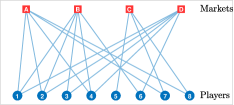
(a)

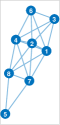
(b)

Figure 1: (a) Interactions of the players $\{1,\dots,8\}$ with the markets $A$, $B$, $C$, $D$, (b) Communication network between players arising from the competition.

The constraint matrix is $\boldsymbol{A}=[A_{1},\dots,A_{N}]\in{\mathbb{R}}^{4\times 32}$ and the columns $k$ of $A_{i}$ have a nonzero element in position $j$ if the $k$-th strategy of player $i$ is applied to market $j$. The nonzero values are randomly chosen from $[0.6,1]$. The elements of $b\in{\mathbb{R}}^{4}$ are the markets’ maximal capacities and are randomly chosen from $[20,100]$. The arising inequality coupling constraint is $\boldsymbol{Ax}\leq b$. The local cost function is $f_{i}(x_{i},\boldsymbol{x}_{-i})=c_{i}(\boldsymbol{x})-P(\boldsymbol{x})^{\top}A_{i}x_{i}$, where $c_{i}(\boldsymbol{x})$ is the cost of playing a certain strategy and $P(\boldsymbol{x})$ the price obtained by the market. We define the markets price as a linear function $P(\boldsymbol{x})=\bar{P}-DA\boldsymbol{x}$, where $\bar{P}\in{\mathbb{R}}^{4}$ and $D\in{\mathbb{R}}^{4\times 4}$ is a diagonal matrix, the values of their elements are randomly chosen respectively from $[250,500]$ and $[1,5]$. The cost function is quadratic $c_{i}(\boldsymbol{x})=x_{i}^{\top}Q_{i}x_{i}+q_{i}^{\top}x_{i}$, where the elements of the diagonal matrix $Q_{i}\in{\mathbb{R}}^{4\times 4}$ and the vector $q_{i}\in{\mathbb{R}}^{4}$ are randomly drawn respectively from $[1,8]$ and $[1,4]$.

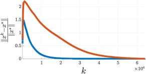
(a)

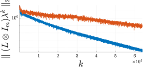
(b)

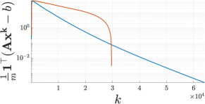
(c)

Figure 2: Communication in alphabetic order (blue) versus random communication (red): (a) Normalized distance from equilibrium,(b) Norm of the disagreement vector, (c) Averaged constraints violation (the negative values are omitted).

We propose two setups, the case of communication over a ring graph with alphabetic order and the case of random communication (in Figure 2, respectively the blue and red trajectories). In the latter, we only ensure that every $20N$ iterations all the agents performed a similar number of updates. The edges of the graph are arbitrarily oriented. We assume that the agents update with uniform probability, i.e., $P[\zeta^{k}=\Upsilon_{i}]=\frac{1}{N}$. The step sizes $\delta,\>\varepsilon,\>\tau$ in AD-GENO are randomly chosen, the first from $[0.5,0.2]$ and the others from $[0.5,0.03]$, in order to ensure $\Phi\succ 0$ and $\eta=0.35$. The maximum delay is assumed $\bar{\varphi}=4$, therefore $\hat{\varpi}^{k}$ in (22) is $\hat{\varpi}^{k}=\mathrm{col}(\hat{\varpi}_{1}^{k},\dots,\hat{\varpi}_{N}^{k})$ where each $\hat{\varpi}_{i}^{k}$ is randomly chosen from $\{\hat{\varpi}_{i}^{k-\bar{\varphi}},\dots,\hat{\varpi}_{i}^{k}\}$.

The results of the simulations are shown in Figure 2. In particular, Figure 2a presents the convergence of the collective strategy $\boldsymbol{x}^{k}$ to the v-GNE $\boldsymbol{x}^{*}$. Furthermore, Figure 2b highlights the convergence of the Lagrangian multipliers to consensus. We noticed that a simple update sequence, as the alphabetically ordered one, leads to a faster convergence than a random one. In general, the more the agents’ updates are well mixed the faster the algorithm converge.

VII Conclusion

This work propose a variant of the forward-backward splitting algorithm to solve generalized Nash equilibrium problems via asynchronous and distributed information exchange, that is robust to communication delays. A change of variables based on the node Laplacian matrix of the information-exchange graph allows one to preserve the scalability of the solution algorithm in the number of nodes (as opposed to the number of edges). Full theoretical and numerical comparison between the proposed solution algorithm and that in [14] is left as future work. Another interesting topic is the adaptation of the algorithm to the case of changing graph topology, in fact the independence from the edge variables makes this approach more suitable to address this problem.

Proof of Lemma 1

It follows as in [5, Proof of Th. 4.5]. ∎

Proof of Theorem 1

Given the equilibrium point $\mathrm{col}(\boldsymbol{x}^{*},\boldsymbol{\lambda}^{*},\boldsymbol{z}^{*})$, (17) evaluated in the equilibrium reduces to $\boldsymbol{0}=\boldsymbol{L}\boldsymbol{\lambda}^{*}$, that implies $\boldsymbol{\lambda}^{*}=\lambda^{*}\otimes\boldsymbol{1}$.

Moreover manipulating (18) and evaluating it in the equilibrium, we obtain

$$\boldsymbol{0}\in N_{{\mathbb{R}}^{mN}_{\geq 0}}(\boldsymbol{\lambda}^{*})+\bar{b}-\Lambda\boldsymbol{x}^{*}+2\boldsymbol{\delta}\boldsymbol{L}\boldsymbol{\lambda}^{*}+\boldsymbol{z}^{*}\,.$$ (23)

Exploiting the property $\boldsymbol{L}\boldsymbol{\lambda}^{*}=\boldsymbol{0}$ and multiplying both side of (23) by $(\boldsymbol{1}^{\top}\otimes I)$ leads to

$$\boldsymbol{0}\in(\boldsymbol{1}^{\top}\otimes I)(N_{{\mathbb{R}}^{mN}_{\geq 0}}(\boldsymbol{\lambda}^{*})+\bar{b}-\Lambda\boldsymbol{x}^{*}+\boldsymbol{z}^{*})\,.$$ (24)

Using the fact that $\sum_{i\in\mathcal{N}}N_{{\mathbb{R}}^{m}_{\geq 0}}(\lambda^{*})=N_{\cap_{i\in\mathcal{N}}{\mathbb{R}}^{m}_{\geq 0}}(\lambda^{*})=N_{{\mathbb{R}}^{m}_{\geq 0}}(\lambda^{*})$ and the assumption $\boldsymbol{1}^{\top}\boldsymbol{z}^{*}=0$, (24) becomes

$$\boldsymbol{0}\in N_{{\mathbb{R}}^{m}_{\geq 0}}(\lambda^{*})+\bar{b}-A\boldsymbol{x}^{*}\,.$$ (25)

Finally, (15) evaluated in the equilibrium is

$$\boldsymbol{0}\in F(\boldsymbol{x}^{*})+N_{\boldsymbol{\Omega}}(\boldsymbol{x}^{*})+\Lambda^{\top}\boldsymbol{\lambda}^{*}\\ \,,$$ (26)

or equivalently

$$\boldsymbol{0}\in\nabla f_{i}(x_{i}^{*},\boldsymbol{x}^{*}_{-i})+N_{\Omega_{i}}(x^{*}_{i})+A_{i}^{\top}\lambda^{*}\>,\quad\forall i\in\mathcal{N}\,.$$ (27)

Inclusions (27) and (25) are the KKT conditions in (7), hence from [6, Th. 3.1] we conclude that $\mathrm{col}(\boldsymbol{x}^{*},\boldsymbol{\lambda}^{*},\boldsymbol{z}^{*})$ is a v-GNE of the game. ∎

Proof of Theorem 2

First, we note from [5, Lem. 5.6] that the two operators $\Phi^{-1}\mathcal{B}$ and $\Phi^{-1}\mathcal{A}$ are respectively $\frac{\alpha\vartheta}{\ell^{2}}$-cocoercive and maximally monotone. Furthermore, this also implies that $(\textrm{Id}-\Phi^{-1}\mathcal{B})$ is $\frac{\ell^{2}}{2\alpha\vartheta}$-AVG and $\mathrm{J}_{\Phi^{-1}\mathcal{A}}=(\textrm{Id}+\Phi^{-1}\mathcal{A})$ is FNE. Applying [24, Prop. 2.4], we conclude that $T$ is $\frac{2\alpha\vartheta}{4\alpha\vartheta-\ell^{2}}$-AVG. The Krasnosel’skiĭ iteration in (11) converges to $\varpi^{*}\in{\mathrm{fix}}(T)$ if $\eta\in(0,\frac{4\alpha\vartheta-\ell^{2}}{2\alpha\vartheta})$, [22, Th. 5.14].

From the above argument, it holds that $\lim_{k\rightarrow+\infty}\boldsymbol{\sigma}^{k}=\boldsymbol{\sigma}^{*}$, hence $\lim_{k\rightarrow+\infty}\boldsymbol{E}^{\top}\boldsymbol{\sigma}^{k}=\boldsymbol{E}^{\top}\boldsymbol{\sigma}^{*}=:\boldsymbol{z}^{*}$, therefore also $\boldsymbol{z}$ converges. Therefore, we conclude that Algorithm 1 converges to $\mathrm{col}(\boldsymbol{x}^{*},\boldsymbol{\lambda}^{*},\boldsymbol{z}^{*})$. The choice of the initial value $\boldsymbol{z}_{0}=\boldsymbol{0}$, implies that $\boldsymbol{1}^{\top}\boldsymbol{z}^{k}=0$, $\forall k\in{\mathbb{N}}_{\geq 0}$ since its values will in the range of the Laplacian matrix. Finally, applying Theorem 1 we conclude that the equilibrium is the v-GNE of the original game. ∎

Proof of Theorem 3

From the proof of Theorem 2, we know that $T$ is $\frac{2\alpha\vartheta}{4\alpha\vartheta-\ell^{2}}$-AVG, therefore is can be rewritten as $T=(1-\frac{2\alpha\vartheta}{4\alpha\vartheta-\ell^{2}})\textrm{Id}+\frac{2\alpha\vartheta}{4\alpha\vartheta-\ell^{2}}P$, where $P$ is nonexpansive, [22, Prop. 4.35]. By substituting it into (22), we obtain

$$\varpi^{k+1}=\varpi^{k}+\frac{2\eta\alpha\vartheta}{4\alpha\vartheta-\ell^{2}}\zeta^{k}(P-\textrm{Id})\hat{\varpi}^{k}\,.$$ (28)

For (28), we apply [13, Lem. 13 and Lem. 14], to conclude that $\{\varpi^{k}\}_{k\in{\mathbb{N}}_{\geq 0}}$ is bounded and that it converges almost surely to $\varpi^{*}\in{\mathrm{fix}}(P)={\mathrm{fix}}(T)$, for $\frac{2\eta\alpha\vartheta}{4\alpha\vartheta-\ell^{2}}\in(0,\frac{cNp_{\min}}{2\bar{\varphi}\sqrt{p_{\min}}+1}]$ with $p_{\min}:=\min\{p_{i}\}_{i\in\mathcal{N}}$. Since ${\mathrm{fix}}(T)={\mathrm{zer}}(\mathcal{A}+\mathcal{B})$, we conclude from Proposition 1 that $\{\boldsymbol{x}^{k}\}_{k\in{\mathbb{N}}_{\geq 0}}$ converges to the v-GNE of (2) almost surely. ∎

Proof of Theorem 4

The change of auxiliary variables in Algorithm 3 from $\boldsymbol{\sigma}$ to $\boldsymbol{z}$ leads to a different update rule for $\boldsymbol{\lambda}$, instead the one for $\boldsymbol{x}$ remains unchanged. Therefore, if we show that the new update of $\boldsymbol{\lambda}$ is equivalent to the one in Algorithm 2, we can infer the convergence from Theorem 3.

We prove by induction that, given an agent $i$, the update of $\lambda_{i}$ at time $k$ in Algorithm 2 and 3 are equivalent. Note that the two update rules are equivalent if it holds that

$$\tilde{z}_{i}^{k}=([E^{\top}]_{i}\otimes I_{m})\hat{\boldsymbol{\sigma}}^{k}\>,$$ (29)

for every $k>0$ and $i\in\mathcal{N}$.

Base case: Iteration $k$ is the first in which agent $i$ updates its variables. If $k=0$, then $\mu_{i}=\boldsymbol{0}_{m}$ in AD-GENO and $\hat{\boldsymbol{\sigma}}^{0}=\boldsymbol{0}_{mM}$ in E-ADAGNES, hence (29) is trivially verified.

If instead $k>0$, it holds that $z_{i}^{k-\varphi^{k}_{i}}=z_{i}^{0}=\boldsymbol{0}_{m}$, while $\hat{\boldsymbol{\sigma}}^{k}\not=\boldsymbol{0}_{mM}$, since the neighbours of $i$ can update more than once before the first update of $i$. We define for each $j\in\mathcal{N}_{i}$ the set $\mathcal{S}_{j}^{k}$, a $t\in{\mathbb{N}}$ where $t<k$ belongs to $\mathcal{S}_{j}^{k}$ if at the iteration $t$ of the algorithm agent $j$ completes an update. We define the maximum time in $\mathcal{S}_{j}^{k}$ as $m_{j}^{k}:=\max\{t\>|\>t\in\mathcal{S}_{j}^{k}\}$ and $\check{\mathcal{S}}_{j}^{k}:={\mathcal{S}}_{j}^{k}\setminus m_{j}^{k}$. From this definitions, we obtain that

$$([E^{\top}]_{i}\otimes I_{m})\hat{\boldsymbol{\sigma}}^{k}=\textstyle{\sum_{l\in\mathcal{E}^{\mathrm{out}}_{i}}}\sigma_{l}^{0}-\textstyle{\sum_{d\in\mathcal{E}^{\mathrm{in}}_{i}}}\sigma_{d}^{m_{j}^{k}}\>,$$ (30)

where $j$ is the element of $e_{d}$ different from $i$. Furthermore, from the update rule of $\sigma_{d}$ in Algorithm 2, we derive

$$\begin{split}\sigma_{d}^{m_{j}^{k}}&=-\sigma_{l}^{\max\{t\>|\>t\in\check{\mathcal{S}}_{j}^{k}\}}-\eta\delta(\lambda_{j}^{\max\{t\>|\>t\in\check{\mathcal{S}}_{j}^{k}\}}-\lambda_{i}^{0})\\ &=\eta\delta\>\textstyle{\sum_{h\in\check{\mathcal{S}}_{j}^{k}}}\left(\lambda_{i}^{0}-\lambda_{j}^{h}\right)\end{split}$$ (31)

Substituting (31) into (30) leads to

$$\begin{split}([E^{\top}]_{i}\otimes I_{m})\hat{\boldsymbol{\sigma}}^{k}&=\eta\frac{\delta}{2}\left(\left[\textstyle{\sum_{j\in\mathcal{N}_{i}\setminus\{i\}}}|\check{S}_{j}^{k}|\right]\lambda_{i}^{0}\right.\\ &\left.\qquad\qquad-\textstyle{\sum_{j\in\mathcal{N}_{i}\setminus\{i\}}\sum_{h\in\check{\mathcal{S}}_{j}^{k}}}\lambda_{j}^{h}\right)\>.\\ \end{split}$$ (32)

From the definition given in Algorithm 3 of $\mu_{i}$, we attain that $([E^{\top}]_{i}\otimes I_{m})\hat{\boldsymbol{\sigma}}^{k}=\eta\delta\mu_{i}=\tilde{z}_{i}^{k}$, therefore (29) hold.

Induction step: Suppose that (29) holds for some $\bar{k}>0$ that corresponds the latest iteration in which agent $i$ performed the update, i.e. $z_{i}^{\bar{k}}\not=\boldsymbol{0}$.

Consider the next iteration $k$ in which agent $i$ updates, $k>\bar{k}$. Here, $\mathcal{S}_{j}^{k}$ is defined as above, but for time indexes $(\bar{k},k]$. Following a similar reasoning to the previous case, we obtain

$$\begin{split}([E^{\top}]_{i}&\otimes I_{m})\hat{\boldsymbol{\sigma}}^{k}=([E^{\top}]_{i}\otimes I_{m})\hat{\boldsymbol{\sigma}}^{\bar{k}}+\eta\delta\sum_{l\in\mathcal{E}_{i}^{\mathrm{out}}}([E]_{l}\otimes I_{m})\hat{\boldsymbol{\lambda}}^{\bar{k}}\\ &+\eta\delta\left(\left[\textstyle{\sum_{j\in\mathcal{N}_{i}\setminus\{i\}}}|\check{S}_{j}^{k}|\right]\lambda_{i}^{0}-\textstyle{\sum_{j\in\mathcal{N}_{i}\setminus\{i\}}\sum_{h\in\check{\mathcal{S}}_{j}^{k}}}\lambda_{j}^{h}\right)\\ \end{split}$$ (33)

where we used the fact that $l\in\mathcal{E}_{i}^{\mathrm{out}}$ is updated at the same time of $i$. Furthermore, from the induction assumption,

$$\begin{split}([E^{\top}]_{i}\otimes I_{m})\hat{\boldsymbol{\sigma}}^{k}&=z^{\bar{k}}_{i}+\eta\delta\left(\left[\textstyle{\sum_{j\in\mathcal{N}_{i}\setminus\{i\}}}|\check{S}_{j}^{k}|\right]\lambda_{i}^{0}\right.\\ &\qquad\left.-\textstyle{\sum_{j\in\mathcal{N}_{i}\setminus\{i\}}\sum_{h\in\check{\mathcal{S}}_{j}^{k}}}\lambda_{j}^{h}\right)\\ &=z^{\bar{k}}_{i}+\eta\delta\mu_{i}=\tilde{z}^{k}_{i}\>,\end{split}$$ (34)

where the last step holds because in the reading phase of Algorithm 3, we reset to zero the values of $\mu_{i}$, every time $i$ starts an update. Therefore, (29) holds for $k$.

This concludes the proof by induction, showing that the update of $\lambda_{i}$ defined in Algorithm 3 is equivalent to the one in Algorithm 2, for any $k$. Finally, since the pair $(\boldsymbol{x},\boldsymbol{\lambda})$ has an update rule equivalent to the one in E-ADAGNES, the convergence of $\{\boldsymbol{x}\}_{k\in{\mathbb{N}}_{\geq 0}}$ to the v-GNE of the game (2) follows by Theorem 3. ∎

References

• [1] F. Dörfler, J. Simpson-Porco, and F. Bullo, “Breaking the hierarchy: Distributed control and economic optimality in microgrids,” IEEE Trans. on Control of Network Systems, vol. 3, no. 3, pp. 241–253, 2016.
• [2] F. Parise, M. Colombino, S. Grammatico, and J. Lygeros, “Mean field constrained charging policy for large populations of plug-in electric vehicles,” in Proc. of the IEEE Conference on Decision and Control, Los Angeles, California, USA, 2014, pp. 5101–5106.
• [3] S. Grammatico, “Proximal dynamics in multi-agent network games,” IEEE Trans. on Control of Network Systems doi.org/10.1109/TCNS.2017.2754358, 2018.
• [4] S. Martínez, F. Bullo, J. Cortés, and E. Frazzoli, “On synchronous robotic networks – Part i: Models, tasks, and complexity,” IEEE Trans. on Automatic Control, vol. 52, pp. 2199–2213, 2007.
• [5] P. Yi and L. Pavel, “A distributed primal-dual algorithm for computation of generalized nash equilibria via operator splitting methods,” in 2017 IEEE 56th Annual Conference on Decision and Control (CDC), Dec 2017, pp. 3841–3846.
• [6] F. Facchinei, A. Fischer, and V. Piccialli, “On generalized Nash games and variational inequalities,” Operations Research Letters, vol. 35, pp. 159–164, 2007.
• [7] D. P. Bertsekas and J. N. Tsitsiklis, “Some aspects of parallel and distributed iterative algorithms—a survey,” Automatica, vol. 27, no. 1, pp. 3 – 21, 1991.
• [8] ——, Parallel and distributed computation: numerical methods.   Prentice hall Englewood Cliffs, NJ, 1989, vol. 23.
• [9] B. Recht, C. Re, S. Wright, and F. Niu, “Hogwild: A lock-free approach to parallelizing stochastic gradient descent,” in Advances in neural information processing systems, 2011, pp. 693–701.
• [10] P. Combettes and J. Pesquet, “Stochastic quasi-fejér block-coordinate fixed point iterations with random sweeping,” SIAM Journal on Optimization, vol. 25, no. 2, pp. 1221–1248, 2015.
• [11] J. Liu, S. J. Wright, C. Ré, V. Bittorf, and S. Sridhar, “An asynchronous parallel stochastic coordinate descent algorithm,” The Journal of Machine Learning Research, vol. 16, no. 1, pp. 285–322, 2015.
• [12] A. Nedic, “Asynchronous broadcast-based convex optimization over a network,” IEEE Transactions on Automatic Control, vol. 56, no. 6, pp. 1337–1351, 2011.
• [13] Z. Peng, Y. Xu, M. Yan, and W. Yin, “Arock: an algorithmic framework for asynchronous parallel coordinate updates,” SIAM Journal on Scientific Computing, vol. 38, no. 5, pp. A2851–A2879, 2016.
• [14] P. Yi and L. Pavel, “Asynchronous distributed algorithms for seeking generalized Nash equilibria under full and partial decision information,” ArXiv e-prints, Jan. 2018.
• [15] D. Paccagnan, B. Gentile, F. Parise, M. Kamgarpour, and J. Lygeros, “Distributed computation of generalized nash equilibria in quadratic aggregative games with affine coupling constraints,” pp. 6123–6128, Dec 2016.
• [16] A. A. Kulkarni and U. Shanbhag, “On the variational equilibrium as a refinement of the generalized Nash equilibrium,” Automatica, vol. 48, pp. 45Ж55, 2012.
• [17] A. Dreves, F. Facchinei, C. Kanzow, and S. Sagratella, “On the solution of the kkt conditions of generalized nash equilibrium problems,” SIAM Journal on Optimization, vol. 21, no. 3, pp. 1082–1108, 2011.
• [18] G. Belgioioso and S. Grammatico, “On convexity and monotonicity in generalized aggregative games,” IFAC-PapersOnLine, vol. 50, no. 1, pp. 14 338 – 14 343, 2017, 20th IFAC World Congress.
• [19] F. Facchinei and J. Pang, Finite-dimensional variational inequalities and complementarity problems.   Springer Verlag, 2003.
• [20] C. Godsil and G. Royle, Algebraic Graph Theory, ser. Graduate Texts in Mathematics.   Springer Science & Business Media, 2013, vol. 207.
• [21] J. Eckstein, “Splitting methods for monotone operators with applications to parallel optimization,” Ph.D. dissertation, Massachusetts Institute of Technology, 1989.
• [22] H. H. Bauschke, P. L. Combettes et al., Convex analysis and monotone operator theory in Hilbert spaces.   Springer, 2011, vol. 408.
• [23] C.-K. Yu, M. van der Schaar, and A. H. Sayed, “Distributed learning for stochastic generalized nash equilibrium problems,” IEEE Transactions on Signal Processing, vol. 65, no. 15, pp. 3893–3908, 2017.
• [24] P. L. Combettes and I. Yamada, “Compositions and convex combinations of averaged nonexpansive operators,” Journal of Mathematical Analysis and Applications, pp. 55–70, 2015.