On the nodal structure of nonlinear stationary waves on star graphs

Abstract.

We consider stationary waves on nonlinear quantum star graphs, i.e. solutions to the stationary (cubic) nonlinear Schrödinger equation on a metric star graph with Kirchhoff matching conditions at the centre. We prove the existence of solutions that vanish at the centre of the star and classify them according to the nodal structure on each edge (i.e. the number of nodal domains or nodal points that the solution has on each edge). We discuss the relevance of these solutions in more applied settings as starting points for numerical calculations of spectral curves and put our results into the wider context of nodal counting such as the classic Sturm oscillation theorem.

1. Introduction

Sturm’s oscillation theorem [1] is a classic example for how solutions of linear self-adjoint differential eigenvalue problems $D\phi(x)=\lambda\phi(x)$ (where $D$ is a Sturm-Liouville operator) are ordered and classified by the number of nodal points. According to Sturm’s oscillation theorem, the $n$-th eigenfunction, $\phi_{n}$, has $n-1$ nodal points, when the eigenfunctions are ordered by increasing order of their corresponding eigenvalues $\lambda_{1}<\lambda_{2}<\lambda_{3}<\dots$. Equivalently, the number $\nu_{n}$ of nodal domains (the connected domains where $\phi_{n}$ has the same sign) obeys $\nu_{n}=n$ for all $n$.

In higher dimensions, (e.g., for the free Schrödinger equation $-\Delta\phi(\mathbf{x})=\lambda\phi(\mathbf{x})$ on a bounded domain with self-adjoint boundary conditions) the number of nodal domains is bounded from above, $\nu_{n}\leq n$, by Courant’s theorem [2] (see [3] for the case of Schrödinger equation with potential). Furthermore, there is only a finite number of Courant sharp eigenfunctions for which $\nu_{n}=n$, as was shown by Pleijel [4].

In (linear) quantum graph theory one considers the Schrödinger equation with self-adjoint matching conditions at the vertices of a metric graph. Locally, graphs are one-dimensional though the connectivity of the graph allows to mimic some features of higher dimensions. Nodal counts for quantum graphs have been considered for more than a decade [5]. For example, it has been shown in [5] that Courant’s bound applies to quantum graphs as well. Yet, for graphs there are generically infinitely many Courant sharp eigenfunctions [7, 6]. For tree graphs it has been proven that all generic eigenfunctions are Courant sharp, i.e., $\nu_{n}=n$ [8, 9] . In other words, Sturm’s oscillation theorem generalizes to metric trees graphs. It has been proven by one of us that the converse also holds, namely that if the graph’s nodal count obeys $\nu_{n}=n$ for all $n$, then this graph is a tree [10]. When a graph is not a tree, its first Betti number, $\beta:=E-V+1$ is positive. Here, $E,V$ are correspondingly the numbers of graph’s edges and vertices and $\beta$ indicates the number of the graphs independent cycles. In addition to Courant’s bound, the nodal count of a graph is bounded from below, $\nu_{n}\leq n-\beta$ as was shown first in [11]. The actual number of nodal domains may be characterized by various variational methods [12, 13]. Some statistical properties of the nodal count are also known [6], but to date there is no general explicit formula or a full statistical description of the nodal count.

In the present work we present some related results concerning nodal points and nodal domains for nonlinear star graphs (see Figure 1.1).

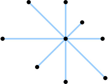
Figure 1.1. A star graph with $E=8$ edges and $E+1=9$ vertices.

Nonlinear wave equations on metric graphs (i.e., nonlinear quantum graphs) have recently attracted considerable interest both from the mathematical perspective and the applied regime. They allow the study of intricate interplay between the non-trivial connectivity and the nonlinearity. Among the physical applications of nonlinear wave equations on metric graphs is light transmission through a network of optical fibres or Bose-Einstein condensates in quasi one-dimensional traps. We refer to [14, 15] where a detailed overview of the recent literature and some applications is given and just summarise here the relevant work related to the nodal counting. In a previous work some of us have shown that Sturm’s oscillation theorem is generically broken for nonlinear quantum stars, apart from the special case of an interval [16]. This is not unexpected as the set of solutions is known to have a far more complex structure. Our main result here is that the nonlinear case of a metric star allows for solutions with any given number of nodal domains on each edge. Namely, for a star with $E$ edges and a certain $E$-tuple, $(n_{1},\dots,n_{E})$ of non-negative integers there are solutions with $n_{e}$ nodal points on the $e$-th edge for $e=1,\,\dots,E$.

In the remainder of the introduction chapter we define the setting. In Section 2 we state our main results. In Section 3 we present the nonlinear generalization of Sturm’s oscillation theorem to an interval, some general background and properties of nonlinear solutions as well as a few motivating numerical results. In Section 4 we prove the main theorems and afterwards in Section 5 we discuss our results and their possible implications in the broader context of nonlinear quantum graphs.

1.1. The Setting—Nonlinear Star Graphs

Metric star graphs are a special class of metric trees with $E$ edges and $E+1$ vertices such that all edges are incident to one common vertex (see Figure 1.1). The common vertex will be called the centre of the star and the other vertices will be called the boundary. We assume that each edge has a finite length $0<\ell_{e}<\infty$ ($e=1,\dots,E$) and a coordinate $x_{e}\in[0,\ell_{e}]$ such that $x_{e}=0$ at the centre and $x_{e}=\ell_{e}$ at the boundary. On each edge $e=1,\dots,E$ we consider the stationary nonlinear Schrödinger (NLS) equation

$$-\frac{d^{2}}{dx_{e}^{2}}\phi_{e}(x_{e})+g|\phi_{e}(x_{e})|^{2}\phi_{e}(x_{e})=\mu\ \phi_{e}(x_{e})$$ (1.1)

for $\phi_{e}\,:\,[0,\ell_{e}]\rightarrow\mathbb{C}$. Here $g$ is a nonlinear coupling parameter and $\mu$ a spectral parameter. We consider this as a generalized eigenequation with eigenvalues $\mu$. We have assumed here that the nonlinear interaction is homogeneously repulsive ($g>0$) or attractive ($g<0$) on all edges and will continue to do so throughout this manuscript. One may consider more general graphs where $g$ takes different values (and different signs) on different edges (or even where $g\rightarrow g_{e}(x_{e})$ is a real scalar function on the graph). It is not, however, our aim to be as general as possible. In the following we restrict ourselves to one generic setting in order to keep the notation and discussion as clear and short as possible. We will later discuss some straightforward generalizations of our results.

At the centre we prescribe Kirchhoff (a.k.a Neumann) matching conditions

$$\phi_{e}(0)= \phi_{e^{\prime}}(0)\quad 1\leq e<e^{\prime}\leq E$$ for all (1.2)

$$\sum_{e=1}^{E}\frac{d\phi_{e}}{dx_{e}}(0)= 0$$ (1.3)

and at the boundary we prescribe Dirichlet conditions $\phi_{e}(\ell_{e})=0$.

For the coupling constant $g$ it is sufficient without loss of generality to consider three different cases. For $g=0$ one recovers the linear Schrödinger equation and thus standard quantum star graphs. For $g=1$ one has a nonlinear quantum star graph with repulsive interaction and for $g=-1$ one has a nonlinear quantum star with attractive interaction. If $g$ takes any other non-zero value a simple rescaling $\phi_{e}(x_{e})\mapsto\frac{1}{\sqrt{|g|}}\phi_{e}(x_{e})$ of the wavefunction is equivalent to replacing $g\mapsto\frac{g}{|g|}=\pm 1$.

Without loss of generality we may focus on real-valued and twice differentiable solutions $\{\phi_{e}(x_{e})\}_{e=1}^{E}$, where twice differentiable refers separately to each $\phi_{e}:(0,\ell_{e})\rightarrow\mathbb{C}$. We also assume that the solution is not the constant zero function on the graph, namely that there is an edge $e$ and some point $\hat{x}_{e}\in[0,\ell_{e}]$ with $\phi_{e}(\hat{x}_{e})\neq 0$. Moreover, any complex-valued solution is related to a real-valued solution by a global gauge-transformation (i.e., a change of phase $\phi_{e}(x_{e})\mapsto\phi_{e}(x_{e})e^{i\alpha}$) [14].

1.2. The Nodal Structure

We will call a solution $\{\phi_{e}(x_{e})\}_{e=1}^{N}$ regular if the wavefunction does not vanish on any edge, that is for each edge $e$ there is $\hat{x}_{e}\in(0,\ell_{e})$ with $\phi_{e}(\hat{x}_{e})\neq 0$. Accordingly, non-regular solutions vanish identically on some edges, in other words there is (at least) one edge $e$ such that $\phi_{e}(x_{e})=0$ for all $x_{e}\in[0,\ell_{e}]$.

A solution with a node at the centre, $\phi_{e}(0)=0$ (by continuity this is either true for all $e$ or for none) will be called central Dirichlet because it satisfies Dirichlet conditions at the centre (in addition to the Kirchhoff condition). Hence, non-regular solutions are always central Dirichlet. Our main theorem will construct solutions which are regular and central Dirichlet. Note that from a regular central Dirichlet solution on a metric star graph $G$ one can construct non-regular solutions on a larger metric star graph $G^{\prime}$, if $G$ is a metric subgraph of $G^{\prime}$: on each edge $e\in G^{\prime}\setminus G$ one may just extend the solution by setting $\phi_{e}(x_{e})=0$ for all $x_{e}\in[0,\ell_{e}]$.

Our main aim is to characterize solutions in terms of their nodal structure. The nodal structure is described in terms of either the number $\nu$ of nodal domains (maximal connected subgraphs where $\phi_{e}(x_{e})\neq 0$) or by the number $\xi$ of nodal points. We will include in the count the trivial nodal points at the boundary. Note that regular solutions which are not central Dirichlet obey $\nu=\xi+1-E$ while regular central Dirichlet solutions obey $\nu=\xi-1$. We have stated in the introduction that in the linear case, $g=0$, such a characterization is very well understood even for the more general tree graphs, which obey a generalized version of Sturm’s oscillation theorem.

As we will see, the solutions of nonlinear star graphs have a very rich structure and a classification of solutions in terms of the total numbers $\nu$ or $\xi$ of nodal domains or nodal points is far from being unique. We will thus use a more detailed description of the nodal structure of the solutions. To each regular solution $\{\phi_{e}(x_{e})\}_{e=1}^{E}$ we associate the $E$-tuple

$$\mathbf{n}=(n_{1},\dots,n_{E})\in\mathbb{N}^{E}$$ (1.4)

where $n_{e}\geq 1$ is the number of nodal domains of the wavefunction $\phi_{e}(x_{e})$ on the edge $x_{e}\in[0,\ell_{E}]$. For solutions which are not central Dirichlet, $n_{e}$ also equals the number of nodal points of $\phi_{e}(x_{e})$ (including the nodal point at the boundary). We will call $\mathbf{n}\in\mathbb{N}^{E}$ the (regular) nodal edge count structure of the (regular) solution $\{\phi_{e}(x_{e})\}_{e=1}^{N}$. For non-regular solutions one may characterize the nodal structure in a similar way by formally setting $n_{e}=\infty$ for all edges where the wavefunction is identical zero. In that case we speak of a non-regular nodal edge count structure. Note that we do not claim that the nodal edge count structure, $\mathbf{n}$, leads to a unique characterization of the solutions (which actually come in one-parameter families). Indeed we have numerical counter-examples. With this more detailed description we show that a much larger set of nodal structures is possible in nonlinear quantum star graphs compared to the linear case, as is stated in the next section.

2. Statement of Main Theorems

Our main results concern the existence of solutions with any given nodal edge structure. We state two theorems: One for repulsive nonlinear interaction $g=1$ and one for attractive nonlinear interaction $g=-1$. The two theorems establish the existence of central Dirichlet solutions with nodal edge structure $\mathbf{n}=(1,\ldots,1)$ subject to (achievable) conditions on the edge lengths. As corollaries, we get the existence of central Dirichlet solutions with any prescribed values of $\mathbf{n}$ (again subject to some achievable conditions on the lengths). Throughout this section we consider a nonlinear quantum star graph as described in Section 1.1. In order to avoid trivial special cases we will assume $E\geq 3$. Indeed, $E=1$ is the interval and well understood and $E=2$ reduces to an interval (of total length $\ell_{1}+\ell_{2}$) as the Kirchhoff vertex condition in this case just states that the wavefunction is continuous and has a continuous first derivative. We will also assume that all edge lengths are different. Without loss of generality we take them as ordered $\ell_{e}<\ell_{e+1}$ ($e=1,\dots,E-1$).

Theorem 2.1.

If $g=1$ (repulsive case) and either

1. the number of edges $E$ is odd, or

2. $E$ is even and

   $$\sqrt{\frac{m_{+}}{m_{-}}}\frac{1+m_{-}}{1+m_{+}}>\frac{E}{E-2},$$ (2.1)

   where $0<m_{-}<m_{+}<1$ are implicitly defined in terms of the edge lengths $l_{1},~{}l_{\frac{E}{2}+1},~{}l_{\frac{E}{2}+2}$ by

   $$\begin{split}K(m_{+})\sqrt{1+m_{+}}=&\frac{\pi}{2}\,\frac{\ell_{\frac{E}{2}+2}}{\ell_{1}},\\ K(m_{-})\sqrt{1+m_{-}}=&\frac{\pi}{2}\,\frac{\ell_{\frac{E}{2}+1}}{\ell_{1}},\end{split}$$ (2.2)

   with

   $$K(m)=\int_{0}^{1}\frac{1}{\sqrt{1-u^{2}}\sqrt{1-mu^{2}}}du$$ (2.3)

   being the complete elliptic integral of first kind,

then there exists a regular central Dirichlet solution for some positive value of the spectral parameter $\mu=k^{2}>\frac{\pi^{2}}{\ell_{1}^{2}}$ such that there is exactly one nodal domain on each edge, i.e., the nodal edge structure $\mathbf{n}$ satisfies $n_{e}=1$ for all edges $e$.

Note that the condition in this theorem for even number of edges involves only three edge lengths and can be stated in terms of two ratios that satisfy $\frac{\ell_{\frac{E}{2}+2}}{\ell_{1}}\geq\frac{\ell_{\frac{E}{2}+1}}{\ell_{1}}\geq 1$ (as we have ordered the edges by lengths). If the larger ratio $\frac{\ell_{\frac{E}{2}+2}}{\ell_{1}}$ is given then one may always achieve this condition by choosing the other ratio sufficiently small (as $\frac{\ell_{\frac{E}{2}+1}}{\ell_{1}}\to 1$ one has $m_{-}\to 0$ and the left-hand side of condition (2.1) grows without any bound). Figure 2.1 shows a graph of the regions where the two length ratios satisfy condition (2.1) for star graphs with $E$ edges. One can see how the condition becomes less restrictive when the number of edges is large. We will present the proof of Theorem 2.1 in Section 4.1. The proof shows that the condition (2.1) is not optimal. Less restrictive conditions that depend on other edge lengths may be stated. Nevertheless, we have chosen to state the condition (2.1), as its form is probably more compactly phrased than other conditions would be.

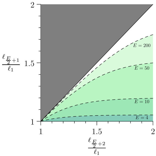
Figure 2.1. The shaded regions indicate choices of relative edge lengths $1<\frac{\ell_{\frac{E}{2}+1}}{\ell_{1}}<\frac{\ell_{\frac{E}{2}+2}}{\ell_{1}}$ that satisfy the condition (2.1) of Theorem 2.1. The dashed lines indicate the boundary of regions for a star graph with $E$ edges (where $E=4,10,50,200$). Condition (2.1) is satisfied below the dashed lines.

Theorem 2.2.

Let $g=-1$ (attractive case). If there exists an integer $M<E/2$ such that

$$\sum_{e=M+1}^{E-1}\frac{1}{\ell_{e}^{2}}<\sum_{e=1}^{M}\frac{1}{\ell_{e}^{2}}<\sum_{e=M+1}^{E}\frac{1}{\ell_{e}^{2}},$$ (2.4)

then there exists a regular central Dirichlet solution for some positive value of the spectral parameter $\mu=k^{2}\in\left(0,\frac{\pi^{2}}{\ell_{E}^{2}}\right)$ such that there is exactly one nodal domain on each edge, i.e., the nodal edge structure $\mathbf{n}$ satisfies $n_{e}=1$ for all edges $e$.

We will prove this theorem in Section 4.2. One may extend Theorem 2.2 to find negative values of the spectral parameter $\mu<0$ under appropriate conditions on edge lengths using similar ideas as the ones used in our proof for $\mu>0$. To keep the paper concise we focus here on $\mu>0$.

In order to demonstrate how the two conditions (2.4) in Theorem 2.2 may be achieved, we point out that the following weaker conditions

$$\begin{split}\frac{\ell_{M}}{\ell_{M+1}}<&\sqrt{\frac{M}{E-M-1}}\\ \frac{\ell_{1}}{\ell_{E}}>&\sqrt{\frac{M}{E-M}}\end{split}$$ (2.5)

imply (2.4) (recalling that $\ell_{1}<\ldots<\ell_{E}$). The conditions (2.5) are easy to apply and they may be achieved straight-forwardly. For instance, if $E$ is odd and $M=(E-1)/2$ (the largest possible value for $M$) then the first inequality in (2.5) is always satisfied and the second condition gives the restriction $1>\frac{\ell_{1}}{\ell_{E}}>\sqrt{\frac{M}{M+1}}$ on the ratio between the smallest and largest edge length. In addition to that one may easily construct a star graph with edge lengths which satisfy conditions (2.5) above. This is done by starting from a star graph which has only two different edge lengths $\ell_{-}<\ell_{+}$ where $\ell_{e}=\ell_{-}$ for $1\leq e\leq M$ and $\ell_{e}=\ell_{+}$ for $M+1\leq e\leq E$. If one chooses the ratio of the lengths in the range $\sqrt{\frac{M}{E-M}}<\frac{\ell_{-}}{\ell_{+}}<\sqrt{\frac{M}{E-M-1}}$ and then perturbs all edge lengths slightly to make them different then condition (2.5) is satisfied. Note however that, just as in Theorem 2.1, even the condition which is stated in Theorem 2.2 is not optimal and more detailed conditions can be derived from our proof in Section 4.2.

Before discussing some straight-forward implications let us also state here that the assumption that all edge lengths are different that we made for both Theorems 2.1 and 2.2 may be relaxed. This is because any two edges with the same length decouple in a certain way from the remaining graph. If one deletes pairs of edges of equal length from the graph until all edges in the remaining graph are different one may apply the theorems to the remaining graph (if the remaining graph has at least three edges). This will be discussed more in Remark 4.1.

In the remainder of this section we discuss the implications of the two theorems for finding solutions with a given nodal edge structure $\mathbf{n}\in\mathbb{N}^{E}$. In this case we divide each edge length into $n_{e}$ fractions $\ell_{e}=n_{e}\tilde{\ell}_{e}$. The $n$-th fraction $\tilde{\ell}_{e}$ then corresponds to the length of one nodal domain. For the rest of this section we do not assume that the edge lengths $\{\ell_{e}\}$ are ordered by length and different, rather we now assume that these assumptions apply to the fractions, i.e., $\tilde{\ell}_{e}<\tilde{\ell_{e+1}}$ ($e=1,\dots,E-1$). By first considering the metrically smaller star graph with edge lengths $\{\tilde{\ell}_{e}\}$ Theorems 2.1 and 2.2 establish the existence of solutions on this smaller graph subject to conditions on the lengths $\{\tilde{\ell}_{e}\}$. These solutions can be extended straight-forwardly to a solution on the full star graph. Indeed, as we explain in more detail in Section 3.1, the solution on each edge is a naturally periodic function given by an elliptic deformation of a sine and shares the same symmetry around nodes and extrema, as the sine function. The main relevant difference to a sine is that the period of the solution depends on the amplitude. In the repulsive case one then obtains the following.

Corollary 2.3.

Let $g=1$ (repulsive case) and $\mathbf{n}\in N^{E}$. If either

1. $E$ is odd, or

2. $E$ is even and the fractions $\tilde{\ell}_{e}=\ell_{e}/n_{e}$ ($e=1,\dots,E$) satisfy the condition (2.1),

then there exists a regular central Dirichlet solution for some positive value of the spectral parameter $\mu=k^{2}>\frac{\pi^{2}}{\tilde{\ell}_{1}^{2}}$ ‘with regular nodal edge count structure $\mathbf{n}$.

Similarly, Theorem 2.2 implies the following.

Corollary 2.4.

Let $g=-1$ (attractive case) and $\mathbf{n}\in\mathbb{N}^{E}$. If the fractions $\tilde{\ell}_{e}=\ell_{e}/n_{e}$ satisfy condition (2.4) then there exists a regular central Dirichlet solution for some positive value of the spectral parameter $\mu=k^{2}\in\left(0,\frac{\pi^{2}}{{\tilde{\ell}_{E}}^{2}}\right)$ with regular nodal edge count structure $\mathbf{n}$.

The corollaries above provide sufficient conditions for the existence of a central Dirichlet solution with a particular given nodal edge count. In addition to that, it is straight-forward to apply Theorems 2.1 and 2.2 to show that for any choice of edge lengths there are infinitely many $E$-tuples which can serve as the graph’s regular central Dirichlet nodal structure.

Moreover Theorems 2.1 and 2.2 also imply infinitely many values for non-regular nodal structures, as every non-regular solution is equivalent to a regular solution on a subgraph.

Finally, we note that the proofs of Theorems 2.1 and 2.2 in Section 4 are constructive and they specify the corresponding solution up to a single parameter (which one may take to be $k=\sqrt{\mu}$) that may easily be found numerically.

3. General Background on the Solutions of Nonlinear Quantum Star Graphs

Before we turn to the proof of Theorems 2.1 and 2.2 we would like discuss how the implied regular central Dirichlet solutions are related to the complete set of solutions of the nonlinear star graph. Though we are far from having a full understanding of all solutions we can give a heuristic picture.

3.1. The Nonlinear Interval - Solutions and Spectral Curves

Let us start with giving a complete overview of the solutions for the interval (i.e., the star graph with $E=1$). While these are well known and understood they play a central part in the construction of central Dirichlet solutions for star graphs in our later proof and serve as a good way to introduce some general background. On the half line $x\geq 0$ with a Dirichlet condition $\phi(0)=0$ at the origin it is straight-forward to check (see also [14]) that the solutions for positive spectral parameters $\mu=k^{2}$ (where $k>0$) are of the form

$$\phi(x)=\begin{cases}\chi_{m,k}^{(+)}(x)=k\sqrt{\frac{2m}{1+m}}\ \mathrm{sn}\left(\frac{kx}{\sqrt{1+m}},m\right)&\text{in the repulsive case $g=1$ ,}\\[5.69046pt] \chi_{m,k}^{(-)}(x)=k\sqrt{\frac{2m(1-m)}{1-2m}}\ \frac{\mathrm{sn}\left(\frac{kx}{\sqrt{1-2m}},m\right)}{\mathrm{dn}\left(\frac{kx}{\sqrt{1-2m}},m\right)}&\text{in the attractive case $g=-1$.}\end{cases}$$ (3.1)

Here $\mathrm{sn}(y,m)$ and $\mathrm{dn}(y,m)$ are Jacobi elliptic functions with a deformation parameter $m$. The definition of elliptic functions allows $m$ to take arbitrary values in the interval $m\in[0,1]$ (as there are many conventions for these functions we summarize ours in Appendix A). Note that $\mathrm{sn}(y,m)$ is a deformed variant of the sine function and $\mathrm{sn}(y,0)=\sin(y)$ and $\mathrm{dn}(y,0)=1$.
For any spectral parameter $\mu=k^{2}$ there is a one-parameter family of solutions parameterised by the deformation parameter $m$. In the repulsive case the deformation parameter may take values $m\in(0,1]$ (as for $m=0$ one obtains the trivial solution $\chi_{0,k}^{(+)}(x)=0$) and in the attractive case $m\in\left(0,\frac{1}{2}\right)$ (the expressions are not well defined for $m=\frac{1}{2}$ and for $m>\frac{1}{2}$ the expressions are no longer real).

Let us now summarise some properties of these solutions in the following proposition for the solutions of the NLS equation on the half line.

Proposition 3.1.

The solutions $\phi(x)=\chi_{m,k}^{(\pm)}(x)$ given in Equation (3.1) have the following properties

1. All solutions are periodic $\chi_{m,k}^{(\pm)}(x)=\chi_{m,k}^{(\pm)}(x+\Lambda^{(\pm)}(m,k))$ with a nonlinear wavelength

   $$\begin{split}\Lambda^{(+)}(m,k)=&\frac{4\sqrt{1+m}K(m)}{k}\\[8.5359pt] \Lambda^{(-)}(m,k)=&\frac{4\sqrt{1-2m}K(m)}{k},\end{split}$$ (3.2)

   where $K(m)$ is the complete elliptic integral of first kind, Equation (2.3).

2. For $m\to 0$ one regains the standard relation $\Lambda^{(\pm)}(0,k)=\frac{2\pi}{k}$ for the free linear Schrödinger equation. In the repulsive case $\Lambda^{(+)}(m,k)$ is an increasing function of $m$ (at fixed $k$) that increases without bound as $m\to 1$. In the attractive case $\Lambda^{(-)}(m,k)$ is a decreasing function of $m$ (at fixed $k$) with $\Lambda^{(-)}\left(\frac{1}{2},k\right)=0$.

3. The nodal points are separated by half the nonlinear wavelength. Namely, $\chi_{m,k}^{(\pm)}(n\Lambda^{(\pm)}(m,k)/2)=0$ for $n=0,1,,\dots$.

4. The solutions are anti-symmetric around each nodal point and symmetric around each extremum, i.e., it has the same symmetry properties as a sine function.

5. As $\mathrm{sn}\left(K(m),m\right)=1$ and $\mathrm{dn}\left(K(m),m\right)=\sqrt{1-m}$ the amplitude

   $$A^{(\pm)}(k,m)=\max\left(\chi_{m,k}^{(\pm)}(x)\right)_{x\geq 0}=\chi_{m,k}^{(\pm)}\left(\frac{\Lambda^{(\pm)}(m,k)}{4}\right)$$

   is given by

   $$\begin{split}A^{(+)}(m,k)=&k\sqrt{\frac{2m}{1+m}}\\[8.5359pt] A^{(-)}(m,k)=&k\sqrt{\frac{2m}{1-2m}}.\end{split}$$ (3.3)

6. As $m\to 0^{+}$ the amplitude of the solutions also decreases to zero $A^{(\pm)}(0,k)=0$ for both the repulsive and the attractive case. In this case the effective strength of the nonlinear interaction becomes weaker and the oscillations are closer. In the repulsive case the amplitude remains bounded as $m\to 1$ with $A^{(+)}(1,k)=k$. In the attractive case $A^{(-)}(m,k)$ grows without bound as $m\to\frac{1}{2}$.

All statements in this proposition follow straight-forwardly from the known properties of elliptic integrals and elliptic functions and we thus omit the proof here. Furthermore, some of the statements in the proposition are mentioned explicitly in [16, 14, 17] and others follow easily from the definitions as given in the Appendix A.

For the NLS equation for $\phi(x)$ on an interval $x\in[0,\ell]$ with Dirichlet conditions at both boundaries $\phi(0)=\phi(\ell)=0$ one obtains a full set of solutions straight-forwardly from the solutions $\chi^{(\pm)}_{m,k}(x)$ on the half-line by requiring that there is a nodal point at $x=\ell$. Since the distance between two nodal points in $\chi^{(\pm)}_{m,k}(x)$ is $\Lambda^{(\pm)}(k,m)/2$ the length of the interval has to be an integer multiple of half the nonlinear wavelength

$$2\ell=n\Lambda^{(\pm)}(k,m),$$ (3.4)

where the positive integer $n$ is the number of nodal domains. We arrive at the following proposition.

Proposition 3.2.

The NLS Equation (1.1) on an interval of length $\ell$ with Dirichlet boundary conditions has a one-parameter family of real-valued solutions with $n$ nodal domains, for each $n\in\mathbb{N}$. The relation between the spectral parameter $\mu=k^{2}$ and the deformation parameter $m$ is dictated by Equation (3.4) and may be explicitly written as

$$\begin{split}k^{(+)}_{n,\ell}(m)=&\frac{2n\sqrt{1+m}K(m)}{\ell}\\[8.5359pt] k^{(-)}_{n,\ell}(m)=&\frac{2n\sqrt{1-2m}K(m)}{\ell}\end{split}.$$ (3.5)

We refer to $k^{(\pm)}_{n\ell}(m)$ (or its implicitly defined inverse $m^{(\pm)}_{n,\ell}(k)$) as spectral curves. As $k^{(\pm)}_{n+1,\ell}(m)>k^{(\pm)}_{n,\ell}(m)$, the spectral curves never cross (see Figure 3.1) and we obtain the first nonlinear generalization of Sturm’s oscillation theorem as a corollary (see also Theorem 2.4 in [16]).

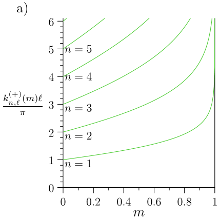
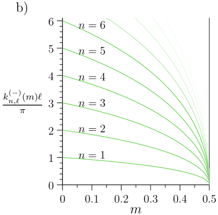
Figure 3.1. Spectral curves $k^{(\pm)}_{n,\ell}(m)$ for the repulsive (a) and attractive case (b). The $n$-th curve is obtained from the curve for $n=1$ by rescaling $k^{(\pm)}_{n,\ell}(m)=nk^{(\pm)}_{1,\ell}(m)$.

Corollary 3.3.

For any allowed value of the deformation parameter $m$ ($m\in(0,1)$ for $g=1$ and $m\in\left(0,\frac{1}{2}\right)$ for $g=-1$) there is a discrete set $\{k_{n}\}_{n=1}^{\infty}$ of positive real numbers, increasingly ordered, such that $\phi_{n}=\left.\chi^{(\pm)}_{m,k_{n}}\right|_{[0,\ell]}$ is a solution of the NLS equation on the interval $[0,\ell]$ with spectral parameters $\mu_{n}=k_{n}^{2}$ and $n$ is the number of nodal domains. Furthermore, these are all the solutions of the NLS equation whose deformation parameter equals $m$.

While this is mathematically sound, fixing the deformation parameter $m$ is not a very useful approach in an applied setting. A more physical approach (and one that is useful when we consider star graphs) is to fix the $L^{2}$-norm $N^{(\pm)}_{n,\ell}(m)=\int_{0}^{\ell}\chi^{(\pm)}_{m,k^{(\pm)}_{n,\ell}(m)}(x)^{2}dx$ of the solutions. The $L^{2}$-norm is a global measure for the strength of the nonlinearity. It has the physical meaning of an integrated intensity. In optical applications this is proportional to the total physical energy and for applications in Bose-Einstein condensates this is proportional to the number of particles.

By direct calculation (see [15]) we express the $L^{2}$-norms in terms of elliptic integrals (see Appendix A) as

$$\begin{split}N^{(+)}_{n,\ell}(m)=&\frac{8n^{2}}{\ell}\ K(m)\left[K(m)-E(1,m)\right]\\[8.5359pt] N^{(-)}_{n,\ell}(m)=&\frac{8n^{2}(1-m)}{\ell}\ K(m)\left[\Pi(1,m,m)-K(m)\right],\end{split}$$ (3.6)

and use those to implicitly define the spectral curves in the form $k^{(\pm)}_{n,\ell}(N)$. The latter spectral curves are shown in Figure 3.2. The monotonicity of the spectral curves in this form follows from the monotonicity of $k^{(\pm)}_{n,\ell}(m)$ together with the monotonicity of $N^{(\pm)}_{n,\ell}(m)$. More precisely, one may check that $N^{(\pm)}_{n,\ell}(m)$ in (3.6) is an increasing function of $m$ in the corresponding interval $m\in(0,1]$ for $g=1$ and $m\in\left(0,\frac{1}{2}\right)$ for $g=-1$. To verify this statement, observe that

1. $\left[K(m)-E(1,m)\right]$ and $\frac{1}{m}\left[\Pi(1,m,m)-K(m)\right]$ are increasing functions of $m$. This follows from their integral representations (see Appendix A). Explicitly, writing each expression as an integral, the corresponding integrands are positive and pointwise increasing functions of $m$.

2. $K(m)$ and $m(1-m)$ are also positive increasing functions of $m$ in the relevant intervals.

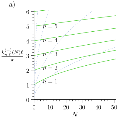
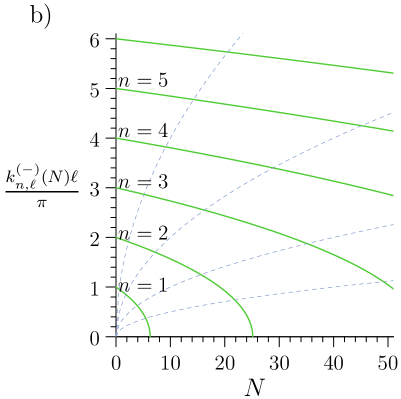
Figure 3.2. The spectral curves $k^{(\pm)}_{n,\ell}(N)$ (full green lines) in the repulsive (a) and attractive case (b). The $n$-th curve is obtained from the curve for $n=1$ by scaling $k^{(\pm)}_{n,\ell}(N)=nk^{(\pm)}_{1,\ell}(N/n^{2})$. The (blue) dashed lines indicate trajectories of the flow (3.8). The deformation parameter $m$ is constant along the flow.

The inverse of $N^{(\pm)}_{n,\ell}(m)$ will be denoted $m^{(\pm)}_{n,\ell}(N)$. Combining the monotonicity of $k^{(\pm)}_{n,\ell}(m)$ and $N^{(\pm)}_{n,\ell}(m)$ one finds in the repulsive case that $k^{(+)}_{n,\ell}(N)$ is an increasing function of $N$ defined for $N>0$ while in the attractive case $k^{(-)}_{n,\ell}(N)$ is a decreasing function defined on $0<N<N_{n,\ell}^{(-),\mathrm{max}}$ where

$$N_{n,\ell}^{(-),\mathrm{max}}=\frac{4n^{2}}{\ell}K\left(\frac{1}{2}\right)\left[\Pi\left(1,\frac{1}{2},\frac{1}{2}\right)-K\left(\frac{1}{2}\right)\right]\ .$$ (3.7)

A characterization of the spectral curves $k^{(\pm)}_{n,\ell}(N)$ may be given as follows. We define the following flow in the $k$-$N$-plane (see Figure 3.2).

$$\Phi^{\tau}(m)=(N^{(\pm)}_{\tau,\ell}(m),k^{(\pm)}_{\tau,\ell}(m)),$$ (3.8)

where $N^{(\pm)}_{\tau,\ell}(m)$ and $k^{(\pm)}_{\tau,\ell}(m)$ are extensions of the expressions in Equations (3.6) and (3.5), replacing the integer valued $n$ with the real flow parameter $\tau$. Observe that $k^{(\pm)}_{\tau,\ell}(m)$ depends linearly on $\tau$ whereas, $N^{(\pm)}_{\tau,\ell}(m)$ is proportional to $\tau^{2}$. This means that for each value of $m$, the corresponding flow line $\left\{\Phi^{\tau}(m)\right\}_{\tau=0}^{\infty}$ is of the form $k=\gamma\sqrt{N}$ (where $\gamma$ depends on $m$). In particular, this implies that the spectral curves $k^{(\pm)}_{n,\ell}(N)$ are self-similar

$$k^{(\pm)}_{n,\ell}(N)=nk^{(\pm)}_{1,\ell}\left(\frac{N}{n^{2}}\right).$$ (3.9)

In addition, each flow line traverses the spectral curves $k^{(\pm)}_{n,\ell}(N)$ in the order given by the number of nodal domains $n$. This implies that the spectral curves never cross each other and remain properly ordered. We thus obtain the following second generalization of Sturm’s oscillation theorem on the interval.

Proposition 3.4.

For $g=1$ (repulsive case) let $N>0$ and for $g=-1$ (attractive case) let $N\in(0,N_{1,\ell}^{(-),\mathrm{max}})$.
Then there is a discrete set $\{k_{n}\}_{n=1}^{\infty}$ of positive real numbers, increasingly ordered such that

$$\phi_{n}=\left.\chi^{(\pm)}_{m^{(\pm)}_{n,\ell}(N),\,k_{n}}\right|_{[0,\ell]}$$

is a solution of the NLS equation on the interval with a spectral parameter $\mu_{n}=k_{n}^{2}$ and $L^{2}$-norm $N=\int_{0}^{\ell}\phi_{n}(x)^{2}\ dx$ and $n$ is the number of nodal domains. Furthermore, these are all solutions whose $L^{2}$-norm equals $N$.

3.2. Nonlinear Quantum Star Graphs

One may use the functions $\chi^{(\pm)}_{m,k}(x)$ defined in Equation (3.1) in order to reduce the problem of finding a solution of the NLS equation on a star graph to a (nonlinear) algebraic problem. By setting

$$\phi_{e}(x_{e})=\sigma_{e}\chi^{(\pm)}_{m_{e},k}(\ell_{e}-x_{e})$$ (3.10)

where an overall sign $\sigma_{e}=\pm 1$ and the deformation parameter $m_{e}$ remain unspecified (and allowed to take different values on different edges) one has a set of $E$ functions that satisfy the NLS equation with spectral parameter $\mu=k^{2}$ on each edge and also satisfy the Dirichlet condition $\phi_{e}(\ell_{e})=0$ at the boundary vertices. Setting $\sigma_{e}=\mathrm{sgn}\left(\chi^{(\pm)}_{m_{e},k}(\ell_{e})\right)$ (unless $\chi^{(\pm)}_{m_{e},k}(\ell_{e})=0$) the Kirchhoff matching conditions at the centre give a set of $E$ independent nonlinear algebraic equations (see Equations (1.2) and (1.3)) for $E$ continuous parameters $\{m_{e}\}$. If $k$ is fixed there are typically discrete solutions for the parameters $\{m_{e}\}$. As $k$ varies the solutions deform and form one-parameter families. Setting

$$N=\sum_{e=1}^{E}\int_{0}^{\ell_{e}}\phi_{e}(x_{e})^{2}\ dx_{e}$$ (3.11)

each solution may be characterized by a pair $(k,N)$ and as $k$ is varied one naturally arrives at spectral curves in the $k$-$N$-plane, that may be expressed as $k(N)$ (or $N(k)$), as we have seen for the interval in the previous section. Nevertheless, the spectral curves of the star graph have a more intricate structure (see Figure 3.3). In non-linear algebraic equations one generally expects that solutions appear or disappear in bifurcations. For any particular example some numerical approach is needed to find the spectral curves. To do so, one first needs to have some approximate solution (either found by analytical approximation or by a numerical search in the parameter space). After that Newton-Raphson methods may be used to find the solution up to the desired numerical accuracy and the spectral curves are found by varying the spectral parameter slowly.

Figure 3.3 shows spectral curves that have been found numerically for a star graph with $E=3$ and edge lengths $\ell_{e}=\sqrt{e}$ ($e=1,2,3$). Most of the curves have been found starting from the corresponding spectrum of the linear problem ($g=0$). Yet, one can see an additional curve that does not connect to the linear spectrum as $N\to 0$. This has originally been found in previous work [15] by coincidence, as the the numerical method jumped from one curve to another where they almost touch in the diagram.

We stress that in a numerical approach it is very hard to make sure that all solutions of interest are found, even if one restricts the search to a restricted region in parameter space. A full characterization of all solutions (such as given above for the nonlinear interval) will generally be elusive even for basic nonlinear quantum graphs. Theorems 2.1 and 2.2 and the related Corollaries 2.3 and 2.4 establish the existence of a large set of solutions inside the deep nonlinear regime. Each of these solutions may be used as a starting point for a numerical calculation of further solutions along the corresponding spectral curves.

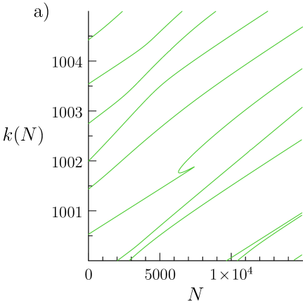
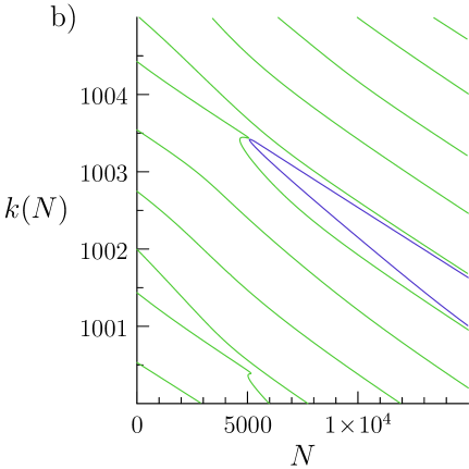
Figure 3.3. Spectral curves $k(N)$ for a nonlinear star graph with $E=3$ edges and edge lengths $\ell_{1}=1$, $\ell_{2}=\sqrt{2}$, and $\ell_{3}=\sqrt{3}$ with repulsive (a) and attractive (b) nonlinear interaction. The spectral curves have been obtained by numerically solving the matching conditions using a Newton-Raphson method. For $N\to 0$ one obtains the spectrum of the corresponding linear star graph. Apart from one curve, all shown curves are connected to the linear spectrum this way. In the attractive case one spectral curve (shown in blue) is not connected to the linear spectrum. Such curves can sometimes be found by coincidence, e.g., if one is close to a bifurcation and numerical inaccuracy allows to jump from one solution branch to another (and this is indeed how we found it). In the repulsive case there is one spectral curve that has a sharp cusp. This indicates that there may be a bifurcation nearby that has additional solution branches that have not been found. In general it is a non-trivial numerical task to ensure that a diagram of spectral curves is complete. Here, completeness has not been attempted as the picture serves a mainly illustrative purpose.

3.3. Nodal Edge Counting and Central Dirichlet Solutions

It is interesting to consider the nodal structure along a spectral curve. Generically the wavefunction does not vanish at the centre and the nodal edge count structure (i.e., the vector $\mathbf{n}$) remains constant along the curve. The existence of central Dirichlet solutions implies that nodal points may move into (and through) the centre along a spectral curve (see also Theorem 2.9, [16]). At this instance the nodal edge count structure changes twice; first when the node hits the centre and then again when it has moved through. If $\mathbf{n}_{0}$ is the nodal edge count structure at a central Dirichlet solution, then generically the value of the function at the centre will change its sign along the spectral curve close to the central Dirichlet solution. If $\mathbf{n}_{<}$ and $\mathbf{n}_{>}$ are the nodal edge count structures close to the central Dirichlet solution then their entries differ at most by one $n_{>,e}-n_{<,e}=\pm 1$ and when the nodal point hits the centre one has $n_{o,e}=\mathrm{min}(n_{>,e},n_{<,e})$. This is shown in more detail for a numerical example in Figure 3.4, where some central Dirichlet solutions are indicated on the spectral curves. The figure also shows the relevance of the central Dirichlet solutions for finding numerical solutions. The central Dirichlet solutions can be constructed directly using the machinery of the proof in the next section. From that one can then obtain a full spectral curve numerically by varying the parameters appropriately.

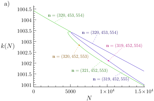
$\left.b\right)$                                                                                                                                  

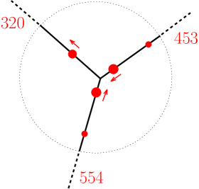
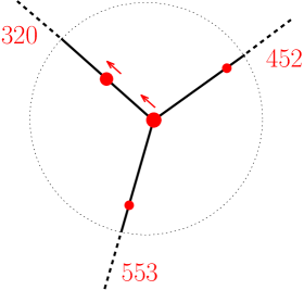
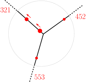
Figure 3.4. Upper panel (a): Two spectral curves (green and blue) of the star graph described in the caption of Figure 3.3 with attractive nonlinear interaction. The yellow and pink dots indicate positions that correspond to central Dirichlet solutions. The nodal edge structure $\mathbf{n}$ is indicated for each part of the curve. The latter is constant along spectral curves apart from jumps at the positions that correspond to central Dirichlet solutions. Lower panel (b): The three diagrams show how the nodal points move through the centre while $N$ is increased through a central Dirichlet point on a spectral curve (the green curve in the upper panel). Only some nodal points close to the centre are shown. In the left diagram the three large dots are the closest to the centre and the arrows indicate how they move when $N$ is increased. The numbers give the number of nodal domains on each edge. Increasing $N$ further two nodal points on different edges merge at the centre as shown in the middle diagram. On the corresponding edges one nodal domain disappears. Further increasing $N$ the nodal point moves from the centre into the remaining edge where the number of nodal domains is increased by one.

4. Proofs of Main Theorems

We prove the two theorems for repulsive and attractive interaction separately. The main construction is however the same. We start by describing the idea behind the construction and then turn to the actual proofs. Let $m^{(\pm)}_{1,\ell_{e}}(k)$ be the functions describing the deformation parameter of solutions on the interval of length $\ell$ with Dirichlet boundary conditions and a single nodal domain (they are given as the inverse of Equation (3.5); see also the lowest curve in Figure 3.1). Those functions are well-defined for $k>\frac{\pi}{\ell_{e}}$ in the repulsive case and for $k<\frac{\pi}{\ell_{e}}$ in the attractive case. Using these, we define

$$\phi_{e}:=\sigma_{e}\left.\chi^{(\pm)}_{m^{(\pm)}_{1,\ell_{e}}(k),\,k}\right|_{[0,\ell_{e}]},$$ (4.1)

for $e=1,\dots,E$, and where $\sigma_{e}=\pm 1$ are signs that will be specified later. These are of course just the solutions of the NLS with one nodal domain on the corresponding interval at spectral parameter $\mu=k^{2}$. In order to ensure that this function is well defined on all edges at given $k$ we have to choose $k\in(\frac{\pi}{\ell_{1}},\infty)$ in the repulsive case and $k\in(0,\frac{\pi}{\ell_{E}})$ in the attractive case (recall that we ordered the edge lengths by $\ell_{1}<\ldots<\ell_{E}$).

As $\phi_{e}(0)=0$ by construction, the set $\left\{\phi_{e}\right\}_{e=1}^{E}$ defines a continuous function on the graph including the centre for all allowed values of $k$. However, in general, these functions do not satisfy the remaining Kirchhoff condition $\sum_{e=1}^{E}\frac{d\phi_{e}}{dx_{e}}(0)=0$. The idea of the proofs is the following. We consider $\sum_{e=1}^{E}\frac{d\phi_{e}}{dx_{e}}(0)$ as a function of $k$ and need to show that it vanishes at some $k=k_{0}$. We find a particular set of signs $\{\sigma_{e}\}$ for which it is easy to show that $\sum_{e=1}^{E}\frac{d\phi_{e}}{dx_{e}}(0)$ changes sign as $k$ is varied within its allowed range. Since this function is continuous in $k$ it must vanish somewhere, which establishes the required central Dirichlet solution with exactly one nodal domain on each edge.

As we recognized above the role which the derivative of the solution plays in the proof, let us now directly calculate it.

$$\theta^{(\pm)}(m):=\frac{1}{\sqrt{2}k^{2}}\frac{d\chi^{(\pm)}_{m,k}}{dx}(0)=\begin{cases}\frac{\sqrt{m}}{1+m}&\text{for $g=1$,}\\[8.5359pt] \frac{\sqrt{m(1-m)}}{1-2m}&\text{for $g=-1$.}\end{cases}$$ (4.2)

In particular, expressing the derivative as a function of $m$ and $k$ and multiplying by a factor $\frac{1}{\sqrt{2}k^{2}}$, we see that the resulting function $\theta^{(\pm)}(m)$ does not depend explicitly on $k$, but only via the deformation parameter, $m$.

Remark 4.1.

In the statement of the theorem we have assumed that all edge lengths are different and stated how this may be relaxed in a subsequent remark. We can explain this now in more detail. Assume that we have two edge lengths that coincide. Denote those edges by $e_{0},e_{1}$ and follow the construction above. By choosing opposite sign for the two edges $\sigma_{e_{0}}=\-\sigma_{e_{1}}$ the contribution of the two edges to the sum of derivatives $\sum_{e=1}^{E}\frac{d\phi_{e}}{dx_{e}}(0)$ cancels exactly for all allowed values of $k$, that is $\frac{d\phi_{e_{0}}}{dx_{e_{0}}}(0)+\frac{d\phi_{e_{1}}}{dx_{e_{1}}}(0)=0$. One may then focus on the subgraph where the two edges are deleted and continue to construct a solution on the subgraph.
One may also start with a graph with different edge lengths. If one has found any regular central Dirichlet solution on the graph one may add as many pairs of edges of the same length and find a regular non-Dirichlet solution on the larger graph following the above construction.

4.1. The Repulsive Case $g=1$

Proof of Theorem 2.1.

Using the construction defined above we have to establish that there is a choice for the signs $\boldsymbol{\sigma}=(\sigma_{1},\dots,\sigma_{E})$ and value for the spectral parameter $k=\sqrt{\mu}$ such that the Kirchhoff condition $\sum_{e=1}^{\infty}\frac{d\phi_{e}}{dx_{e}}(0)=0$ is satisfied. For $k\in(\frac{\pi}{\ell_{1}},\infty)$ let us define the function

$$f_{\boldsymbol{\sigma}}(k):=\sum_{e=1}^{E}\sigma_{e}\theta^{(+)}\left(m^{(+)}_{1,\ell_{e}}(k)\right)=\sum_{e}^{E}\sigma_{e}\frac{\sqrt{m^{(+)}_{1,\ell_{e}}(k)}}{1+m^{(+)}_{1,\ell_{e}(k)}}$$ (4.3)

where $\theta^{(+)}(m)$ was defined in Equation (4.2) and $m^{(+)}_{1,\ell_{e}}(k)$ is the inverse of

$$k^{(+)}_{1,\ell_{e}}(m)=\frac{2}{\ell_{e}}\sqrt{1+m}K(m)$$ (4.4)

as defined in Equation (3.5) (setting $n=1$ for one nodal domain). The Kirchhoff condition is equivalent to the condition $f_{\boldsymbol{\sigma}}(k)=0$ for some $k>\frac{\pi}{\ell_{1}}$.

To continue the proof, we point out some monotonicity properties of $\theta^{(+)}(m)$ and $m^{(+)}_{1,\ell_{e}}(k)$. These properties may be easily verified by direct calculation using Equations (3.5) and (4.2). For $m\in(0,1)$ the functions $\theta^{(+)}(m)$ and $k^{(+)}_{1,\ell_{e}}(m)$ are strictly increasing and

$$\theta^{(+)}(0)=0, \quad\theta^{(+)}(1)=\frac{1}{2},$$ (4.5)

$$k^{(+)}_{1,\ell_{e}}(0)=\frac{\pi}{\ell_{e}}, \quad k^{(+)}_{1,\ell_{e}}(m)\underset{m\to 1}{\longrightarrow}\infty.$$ (4.6)

This implies that $\theta^{(+)}\left(m^{(+)}_{1,\ell_{e}}(k)\right)$ is strictly increasing for $k\in(\frac{\pi}{\ell_{e}},\infty)$ and

$$\theta^{(+)}\left(m^{(+)}_{1,\ell_{e}}\left(\frac{\pi}{\ell_{e}}\right)\right)=0\quad,\quad\theta^{(+)}\left(m^{(+)}_{1,\ell_{e}}(k)\right)\underset{k\to\infty}{\longrightarrow}\frac{1}{2}.$$ (4.7)

If $E\geq 3$ is odd we choose the signs $\boldsymbol{\sigma}=(\sigma_{1},\dots,\sigma_{E})$ to satisfy the following conditions

$$\sigma_{1}=-1\quad\textrm{and}\quad\sum_{e=2}^{E}\sigma_{e}=0$$ (4.8)

and

$$f_{\boldsymbol{\sigma}}\left(\frac{\pi}{\ell_{1}}\right)=\sum_{e=1}^{E}\sigma_{e}\theta^{(+)}\left(m^{(+)}_{1,\ell_{e}}\left(\frac{\pi}{\ell_{1}}\right)\right)>0\ .$$ (4.9)

Such a choice of signs is always possible as $\theta^{(+)}\left(m^{(+)}_{1,\ell_{e}}\left(\frac{\pi}{\ell_{1}}\right)\right)>0$ for all $e>1$. We then get by Equations (4.7) and (4.8) that $\lim_{k\to\infty}f_{\boldsymbol{\sigma}}(k)=\frac{1}{2}\sum_{e=1}^{E}\sigma_{e}=-\frac{1}{2}$. By continuity there exists $k_{0}\in(\frac{\pi}{\ell_{1}},\infty)$ such that $f_{\boldsymbol{\sigma}}(k_{0})=0$ for the given choice of signs. This proves the theorem for odd $E$.

For an even number of edges $E=2M$ ($M\geq 2$) one needs to do a little bit more work. In this case, there are two strategies for choosing signs, $\boldsymbol{\sigma}=(\sigma_{1},\dots,\sigma_{E})$, and showing that $f_{\boldsymbol{\sigma}}\left(k\right)$ vanishes for some $k$.

1. One may choose more negative signs than positive signs so that $\sum_{e}\sigma_{e}<0$. Then $\lim_{k\to\infty}f_{\boldsymbol{\sigma}}\left(k\right)=\frac{1}{2}\sum_{e=1}^{E}\sigma_{e}$ is trivially negative. The difficulty here is in showing that such a choice is consistent with $f_{\boldsymbol{\sigma}}\left(\frac{\pi}{\ell_{1}}\right)>0$. This generally leads to some conditions which the edge lengths should satisfy.

2. One may choose as many positive as negative signs, which makes it easier to satisfy $f_{\boldsymbol{\sigma}}\left(\frac{\pi}{\ell_{1}}\right)>0$ (i.e., the conditions on the edge lengths are less restrictive). Yet, the difficulty here lies in $\lim_{k\to\infty}f_{\boldsymbol{\sigma}}\left(k\right)=0$, which means that one needs to show that this limit is approached from the negative side (i.e., find the conditions on the edge lengths which ensures this).

These two strategies give some indication on how our proof may be generalized beyond the stated length restrictions. Moreover, they also give a practical instruction for how one may search for further solutions numerically.

We continue the proof by following the second strategy and setting

$$\sigma_{e}=\begin{cases}1&\text{for $e=1$ and $e\geq M+2$,}\\ -1&\text{for $2\leq e\leq M+1$}\end{cases}$$ (4.10)

so that $\sum_{e=1}^{E}\sigma_{e}=0$. One then has $\lim_{k\to\infty}f_{\boldsymbol{\sigma}}\left(k\right)=0$ and we will show that the leading term in the (convergent) asymptotic expansion of $f_{\boldsymbol{\sigma}}\left(k\right)$ for large $k$ is negative. Using the known asymptotics [17] of the elliptic integral $K(m)$ as $m=1-\delta m$ goes to one (or $\delta m\to 0$)

$$K(1-\delta m)=-\frac{1}{2}\log(\delta m)+2\log(2)+O\left(\delta m\ \log(\delta m)\right)$$ (4.11)

one may invert Equation (4.4) asymptotically for large $k$ as

$$1-m^{(\pm)}_{1,\ell_{e}}(k)=16e^{-\frac{k\ell_{e}}{\sqrt{2}}}+O\left(ke^{-\sqrt{2}k\ell_{e}}\right)$$ (4.12)

and, thus

$$\begin{split}\frac{\sqrt{m^{(\pm)}_{1,\ell_{e}}(k)}}{1+m^{(\pm)}_{1,\ell_{e}}(k)}=&\frac{\sqrt{1-\left(1-m^{(\pm)}_{1,\ell_{e}}(k)\right)}}{2-\left(1-m^{(\pm)}_{1,\ell_{e}}(k)\right)}\\ =&\frac{1}{2}-\frac{1}{16}\left(1-m^{(\pm)}_{1,\ell_{e}}(k)\right)^{2}+O\left(\left(1-m^{(\pm)}_{1,\ell_{e}}(k)\right)^{3}\right)\\ =&\frac{1}{2}-16e^{-\sqrt{2}k\ell_{e}}+O\left(ke^{-3\frac{k\ell_{e}}{\sqrt{2}}}\right)\ .\end{split}$$ (4.13)

This directly leads to the asymptotic expansion

$$f_{\boldsymbol{\sigma}}(k)=-\sum_{e=1}^{E}\sigma_{e}16e^{-\sqrt{2}k\ell_{e}}+O\left(ke^{-3\frac{k\ell_{1}}{\sqrt{2}}}\right)=-16e^{-\sqrt{2}k\ell_{1}}\left(1+\sum_{e=2}^{E}\sigma_{e}e^{-\sqrt{2}k(\ell_{e}-\ell_{1})}\right)+O\left(ke^{-3\frac{k\ell_{1}}{\sqrt{2}}}\right)$$ (4.14)

which is negative for sufficiently large $k$ because $\ell_{1}$ is the shortest edge length.

It is left to show $f_{\boldsymbol{\sigma}}\left(\frac{\pi}{\ell_{1}}\right)>0$.

For this let us write $m^{(+)}_{1,\ell_{e}}(k)=m^{(+)}_{1,1}(k\ell_{e})$ for each term. As $\theta^{(+)}\left(m^{(+)}_{1,1}\left(\pi\right)\right)=0$ the condition $f_{\boldsymbol{\sigma}}\left(\frac{\pi}{\ell_{1}}\right)>0$ is equivalent to

$$\sum_{e=2}^{M+1}\theta^{(+)}\left(m^{(+)}_{1,1}\left(\frac{\pi\ell_{e}}{\ell_{1}}\right)\right)<\sum_{e=M+2}^{E}\theta^{(+)}\left(m^{(+)}_{1,1}\left(\frac{\pi\ell_{e}}{\ell_{1}}\right)\right),$$ (4.15)

using our choice of the signs, Equation (4.10). Since $m^{(+)}_{1,1}$ and $\theta^{(+)}$ are increasing functions and $\ell_{1}<\ldots<\ell_{E}$, condition (4.15) is certainly satisfied if

$$\frac{\theta^{(+)}\left(m^{(+)}_{1,1}\left(\frac{\pi\ell_{M+2}}{\ell_{1}}\right)\right)}{\theta^{(+)}\left(m^{(+)}_{1,1}\left(\frac{\pi\ell_{M+1}}{\ell_{1}}\right)\right)}>\frac{M}{M-1}\ .$$ (4.16)

The condition (4.16) restricts the three edge lengths $\ell_{1}$, $\ell_{M+1}$ and $\ell_{M+2}$ and it is equivalent to the condition (2.1) stated in the theorem. Indeed, this is trivial for the right-hand side where $\frac{M}{M-1}=\frac{E}{E-2}$. For the left-hand side note that Equation (2.2) in Theorem 2.1 identifies $m_{+}=m^{(+)}_{1,1}\left(\frac{\pi\ell_{M+2}}{\ell_{1}}\right)$ and $m_{-}=m^{(+)}_{1,1}\left(\frac{\pi\ell_{M+1}}{\ell_{1}}\right)$ such that the left-hand-side of the stated condition (2.1) in the theorem and the left-hand side of Equation (4.16) are identical when written out explicitly. ∎

4.2. The Attractive Case $g=-1$

Proof of Theorem 2.2.

In the attractive case we can start similarly to the previous proof by rewriting the Kirchhoff condition on the sum of derivatives as $f_{\boldsymbol{\sigma}}(k)=0$ for some $k\in(0,\frac{\pi}{\ell_{E}})$ where

$$f_{\boldsymbol{\sigma}}(k)=k^{2}\sum_{e=1}^{E}\sigma_{e}\theta^{(-)}\left(m^{(-)}_{1,\ell_{e}}(k)\right)=\sum_{e}^{E}\sigma_{e}\frac{4\sqrt{m^{(-)}_{1,\ell_{e}}(k)(1-m^{(-)}_{1,\ell_{e}}(k))}K\left(m^{(-)}_{1,\ell_{e}}(k)\right)^{2}}{\ell_{e}^{2}}\ .$$ (4.17)

The additional factor $k^{2}$ is irrelevant for satisfying the condition but allows us to extend the definition of the function to $k=0$ (where $k^{2}\sim 1-2m^{(-)}_{1,\ell}(k)$). Noting that $m^{(-)}_{1,\ell_{e}}(k)$ is a decreasing function for $k\in(0,\frac{\pi}{\ell_{e}})$ with $m^{(-)}_{1,\ell_{e}}(0)=\frac{1}{2}$ and $m^{(-)}_{1,\ell_{e}}\left(\frac{\pi}{\ell_{e}}\right)=0$ and $K(m)$ is increasing with $m$ we get that the function

$$k^{2}\theta^{(-)}\left(m^{(-)}_{1,\ell_{e}}(k)\right)=\frac{4\sqrt{m^{(-)}_{1,\ell_{e}}(k)(1-m^{(-)}_{1,\ell_{e}}(k))}K\left(m^{(-)}_{1,\ell_{e}}(k)\right)^{2}}{\ell_{e}^{2}}$$

is a decreasing function for $k\in(0,\frac{\pi}{\ell_{e}})$ and

$$\lim_{k\to 0}k^{2}\theta^{(-)}\left(m^{(-)}_{1,\ell_{e}}(k)\right)=\frac{2K(\frac{1}{2})^{2}}{\ell_{2}^{2}}\quad,\quad\left(\frac{\pi}{\ell_{e}}\right)^{2}\theta^{(-)}\left(m^{(-)}_{1,\ell_{e}}\left(\frac{\pi}{\ell_{e}}\right)\right)=0.$$

Altogether this implies that

$$f_{\boldsymbol{\sigma}}(0)=2K\left(\frac{1}{2}\right)^{2}\sum_{e=1}^{E}\frac{\sigma_{e}}{\ell_{e}^{2}}$$ (4.18)

and

$$f_{\boldsymbol{\sigma}}\left(\frac{\pi}{\ell_{E}}\right)=\sum_{e=1}^{E-1}\sigma_{e}\frac{4\sqrt{m^{(-)}_{1,\ell_{e}}\left(\frac{\pi}{\ell_{E}}\right)\left(1-m^{(-)}_{1,\ell_{e}}\left(\frac{\pi}{\ell_{E}}\right)\right)}K\left(m^{(-)}_{1,\ell_{e}}\left(\frac{\pi}{\ell_{E}}\right)\right)^{2}}{\ell_{e}^{2}}$$ (4.19)

Now let us assume that the two conditions (2.4) stated in Theorem 2.2 are satisfied and let us choose (for $M<E/2$ as is given in the condition of the theorem)

$$\sigma_{e}=\begin{cases}1&\text{for $e\leq M$,}\\ -1&\text{for $e\geq M+1$.}\end{cases}$$ (4.20)

Then

$$f_{\boldsymbol{\sigma}}(0)=2K\left(\frac{1}{2}\right)^{2}\left[\sum_{e=1}^{M}\frac{1}{\ell_{e}^{2}}-\sum_{e=M+1}^{E}\frac{1}{\ell_{e}^{2}}\right]$$ (4.21)

and the right inequality of (2.4) directly implies that $f_{\boldsymbol{\sigma}}(0)<0$.

In order to prove the existence of the solution stated in Theorem 2.2, it is left to show that $f_{\boldsymbol{\sigma}}\left(\frac{\pi}{\ell_{E}}\right)>0$, which would imply that $f_{\boldsymbol{\sigma}}$ vanishes for some $k\in(0,\frac{\pi}{\ell_{E}})$. Using our choice of signs and the identity $m^{(-)}_{1,\ell_{e}}(k)=m^{(-)}_{1,1}(k\ell_{e})$ we may rewrite Equation (4.19) as

$$\begin{split}f_{\boldsymbol{\sigma}}\left(\frac{\pi}{\ell_{E}}\right)=&\sum_{e=1}^{M}\frac{4\sqrt{m^{(-)}_{1,1}\left(\frac{\pi\ell_{e}}{\ell_{E}}\right)\left(1-m^{(-)}_{1,1}\left(\frac{\pi\ell_{e}}{\ell_{E}}\right)\right)}K\left(m^{(-)}_{1,1}\left(\frac{\pi\ell_{e}}{\ell_{E}}\right)\right)^{2}}{\ell_{e}^{2}}\\ -&\sum_{e=M+1}^{E-1}\frac{4\sqrt{m^{(-)}_{1,1}\left(\frac{\pi\ell_{e}}{\ell_{E}}\right)\left(1-m^{(-)}_{1,1}\left(\frac{\pi\ell_{e}}{\ell_{E}}\right)\right)}K\left(m^{(-)}_{1,1}\left(\frac{\pi\ell_{e}}{\ell_{E}}\right)\right)^{2}}{\ell_{e}^{2}}.\end{split}$$ (4.22)

As $\sqrt{m(1-m)}K(m)^{2}$ is an increasing function for $m\in(0,\frac{1}{2})$ and $m^{(-)}_{1,1}(k)$ is a decreasing function of its argument the left inequality in Equation (2.4) implies

$$\sqrt{m_{-}\left(1-m_{-}\right)}K\left(m_{-})\right)^{2}\sum_{e=M+1}^{E-1}\frac{1}{\ell_{e}^{2}}<\sqrt{m_{+}\left(1-m_{+}\right)}K\left(m_{+})\right)^{2}\sum_{e=1}^{M}\frac{1}{\ell_{e}^{2}}$$ (4.23)

where $m_{+}=m^{(-)}_{1,1}\left(\frac{\pi\ell_{M}}{\ell_{1}}\right)$ and $m_{-}=m^{(-)}_{1,1}\left(\frac{\pi\ell_{M+1}}{\ell_{1}}\right)$. The same monotonicity argument implies that the negative contributions in Equation (4.22) are smaller than the left-hand side of inequality Equation (4.23) and that the positive contributions in Equation (4.22) are larger than the right-hand side of inequality Equation (4.23). Thus Equation (4.23) implies $f_{\boldsymbol{\sigma}}\left(\frac{\pi}{\ell_{E}}\right)>0$, as required. ∎

5. Conclusions

We have established the existence of solutions of the stationary nonlinear Schrödinger equation on metric star graphs with a nodal point at the centre. The existence is subject to certain conditions on the edge lengths that can be satisfied for any numbers of edges $E\geq 3$. We stress that some of these solutions are deep in the nonlinear regime where finding any solutions is quite non-trivial. Let us elaborate on that. The non-linear solutions come in one-parameter families, and a possible way to track those families (or curves) is to start from the solutions of the corresponding linear Schrödinger equation. Indeed, since the linear solutions are good approximations for the nonlinear solutions with low intensities they may be used as starting points for finding nonlinear solutions numerically. By slowly changing parameters one may then find some spectral curves that extend into the deep nonlinear regime. However, there may be many solutions on spectral curves that do not extend to arbitrary small intensities and these are are much harder to find numerically. By focusing on solutions which vanish at the centre our work shows how to construct such solutions. These may then be used in a numerical approach to give a more complete picture of spectral curves.

The solutions that we construct are characterised by their nodal count structure. The nodal structure on a spectral curve is constant as long as the corresponding solutions do not vanish at the centre. Our approach thus constructs the solutions where the nodal structure changes along the corresponding spectral curve. In this way we have made some progress in characterizing general solutions on star graphs in terms of their nodal structure.

Many open questions remain. The main one being whether all spectral curves of the NLS equation on a star graph may be found just by combining the linear solutions with the non-linear solutions which vanish at the centre. If not, how many other spectral curves remain and how can they be characterized? Numerically we found that apart from the ground state spectral curve it is generic for a spectral curve to have at least one point where the corresponding solution vanishes at the centre. Of course this leaves open how many spectral curves there are where the corresponding solutions never vanishes at the centre. Another interesting line of future research may be to extend some of our results to tree graphs.

Acknowledgments

R.B. and A.J.K. were supported by ISF (Grant No. 494/14). S.G. would like to thank the Technion for hospitality and the Joan and Reginald Coleman-Cohen Fund for support.

Appendix A Elliptic Integrals and Jacobi Elliptic Functions

We use the following definitions for elliptic integrals (the Jacobi form)

$$F(x|m):= \int_{0}^{x}\frac{1}{\sqrt{1-u^{2}}\sqrt{1-m\,u^{2}}}du$$ (A.1a)

$$K(m):= F(1|m)$$ (A.1b)

$$E(x|m):= \int_{0}^{x}\frac{\sqrt{1-m\,u^{2}}}{\sqrt{1-u^{2}}}du$$ (A.1c)

$$\Pi(x|a,m):= \int_{0}^{x}\frac{1}{\sqrt{1-u^{2}}\sqrt{1-m\,u^{2}}(1-a\,u^{2})}du$$ (A.1d)

where $0\leq x\leq 1$, $m\leq 1$ and $a\leq 1$. Note that our definition allows $m$ and $a$ to be negative.

The notation in the literature is far from being uniform. Our choice seems the most concise for the present context and it is usually straight-forward to translate our definitions into the ones of any standard reference on special functions. For instance, the NIST Handbook of Mathematical Functions [17] defines the three elliptical integrals $F(\phi,k)$, $E(\phi,k)$ and $\Pi(\phi,\alpha,k)$ by setting $x=\sin(\phi)$, $m=k^{2}$, and $a=\alpha^{2}$ in our definitions above.

Jacobi’s Elliptic function $\mathrm{sn}(x,m)$, the elliptic sine, is defined as the inverse of $F(u|m)$

$$u=\mathrm{sn}(x,m)\qquad\Leftrightarrow\qquad x=F(u|m)\ .$$ (A.2)

This defines $\mathrm{sn}(x,m)$ for $x\in[0,K(m)]$ which can straight-forwardly be extended to a periodic function with period $4K(m)$ by requiring $\mathrm{sn}(K(m)+x,m)=\mathrm{sn}(K(m)-x,m)$, $\mathrm{sn}(-x,m)=-\mathrm{sn}(x,m)$ and $\mathrm{sn}(x+4K(m),m)=\mathrm{sn}(x,m)$. The corresponding elliptic cosine $\mathrm{cn}(x,m)$ is obtained by requiring that it is a continuous function satisfying

$$\mathrm{cn}^{2}(x,m)+\mathrm{sn}^{2}(x,m)=1$$ (A.3)

such that $\mathrm{cn}(0,m)=1$. It is useful to also define the non-negative function

$$\mathrm{dn}(x,m):=\sqrt{1-m\,\mathrm{sn}^{2}(x,m)}.$$ (A.4)

At $m=0$ and $m=1$ the elliptic functions can be expressed as

$$\mathrm{sn}(x,0)= \sin x, \mathrm{sn}(x,1)= \tanh x,$$ (A.5a)

$$\mathrm{cn}(x,0)= \cos x, \mathrm{cn}(x,1)= \cosh^{-1}x,$$ (A.5b)

$$\mathrm{dn}(x,0)= 1, \mathrm{dn}(x,1)= \cosh^{-1}x\ .$$ (A.5c)

Derivatives of elliptic functions can be expressed in terms of elliptic functions

$$\frac{d}{dx}\mathrm{sn}(x,m)= \mathrm{cn}(x,m)\mathrm{dn}(x,m),$$ (A.6a)

$$\frac{d}{dx}\mathrm{cn}(x,m)= -\mathrm{sn}(x,m)\mathrm{dn}(x,m),$$ (A.6b)

$$\frac{d}{dx}\mathrm{dn}(x,m)= -m\,\mathrm{sn}(x,m)\mathrm{cn}(x,m)\ .$$ (A.6c)

The first of these equations implies that $u=\mathrm{sn}(x,m)$ is a solution of the first order ordinary differential equation

$$\frac{du}{dx}=\sqrt{1-u^{2}}\sqrt{1-mu^{2}}\ .$$ (A.7)

References

- [1] Sturm, C. Mémoire sur une classe d’équations à différences partielles. J. Math. Pures Appl. 1836, 1, 373–444.
- [2] Courant, R. Ein allgemeiner Satz zur Theorie der Eigenfunktionen selbstadjungierter Differentialausdrücke. Nachr. Ges. Wiss. Göttingen Math Phys. 1923, K1, 81–84.
- [3] Ancona, A.; Helffer, B.; Hoffmann-Ostenhof, T. Nodal domain theorems à la Courant. Doc. Math. 2004, 9, 283–299.
- [4] Pleijel, A. Remarks on courant’s nodal line theorem. Commun. Pure Appl. Math. 1956, 9, 543–550.
- [5] Gnutzmann, S.; Smilansky, U.; Weber, J. Nodal counting on quantum graphs. Waves Random Med. 2004, 14, S61–S73.
- [6] Alon, L.; Band, R.; Berkolaiko, G. Nodal statistics on quantum graphs. Commun. Math. Phys. 2018, 362, 909–948.
- [7] Band, R.; Berkolaiko, G.; Weyand, T. Anomalous nodal count and singularities in the dispersion relation of honeycomb graphs. J. Math. Phys. 2015, 56, 122111.
- [8] Pokornyĭ, Y.V.; Pryadiev, V.L.; Al’-Obeĭd, A. On the oscillation of the spectrum of a boundary value problem on a graph. Mat. Zametki 1996, 60, 468–470.
- [9] Schapotschnikow, P. Eigenvalue and nodal properties on quantum graph trees. Waves Random Complex Med. 2006, 16, 167–78.
- [10] Band, R. The nodal count implies the graph is a tree. Philos. Trans. R. Soc. Lond. A 2014, 372, 20120504, doi:10.1098/rsta.2012.0504.
- [11] Berkolaiko, G. A lower bound for nodal count on discrete and metric graphs. Commun. Math. Phys. 2007, 278, 803–819.
- [12] Band, R.; Berkolaiko, G.; Raz, H.; Smilansky, U. The number of nodal domains on quantum graphs as a stability index of graph partitions. Commun. Math. Phys. 2012, 311, 815–838.
- [13] Berkolaiko, G.; Weyand, T. Stability of eigenvalues of quantum graphs with respect to magnetic perturbation and the nodal count of the eigenfunctions. Philos. Trans. R. Soc. A 2013, 372, doi:10.1098/rsta.2012.0522.
- [14] Gnutzmann, S.; Waltner, D. Stationary waves on nonlinear quantum graphs: General framework and canonical perturbation theory. Phys. Rev. 2016, doi:10.1103/PhysRevE.93.032204.
- [15] Gnutzmann, S.; Waltner, D. Stationary waves on nonlinear quantum graphs: II. application of canonical perturbation theory in basic graph structures. Phys. Rev. E 2016, 94, doi:10.1103/PhysRevE.94.062216.
- [16] Band, R.; Krueger, A.J. Nonlinear Sturm oscillation: From the interval to a star. In Mathematical Problems in Quantum Physics; American Mathematical Society: Providence, RI, USA, 2018; Volume 717, pp. 129–154.
- [17] Olver, F.W.J.; Lozier, D.W.; Boisvert, R.F.; Clark, C.W. The NIST Handbook of Mathematical Functions; Cambridge Univ. Press: Cambridge, UK, 2010.