Models of irradiated molecular shocks

Abstract

Context. The recent discovery of excited molecules in starburst galaxies observed with ALMA and the Herschel space telescope has highlighted the necessity to understand the relative contributions of radiative and mechanical energies in the formation of molecular lines and explore the conundrum of turbulent gas bred in the wake of galactic outflows.

Aims. The goal of the paper is to present a detailed study of the propagation of low velocity (5 to 25 km s^-1) stationary molecular shocks in environments illuminated by an external ultraviolet (UV) radiation field. In particular, we intend to show how the structure, dynamics, energetics, and chemical properties of shocks are modified by UV photons and to estimate how efficiently shocks can produce line emission.

Methods. We implemented several key physico-chemical processes in the Paris-Durham shock code to improve the treatment of the radiative transfer and its impact on dust and gas particles. We propose a new integration algorithm to find the steady-state solutions of magnetohydrodynamics equations in a range of parameters in which the fluid evolves from a supersonic to a subsonic regime. We explored the resulting code over a wide range of physical conditions, which encompass diffuse interstellar clouds and hot and dense photon-dominated regions (PDR).

Results. We find that C-type shock conditions cease to exist as soon as $G_{0}>0.2\,\,({n_{\rm H}}/{\,{\rm cm}^{-3}})^{1/2}$. Such conditions trigger the emergence of another category of stationary solutions, called C*-type and CJ-type shocks, in which the shocked gas is momentarily subsonic along its trajectory. These solutions are shown to be unique for a given set of physical conditions and correspond to dissipative structures in which the gas is heated up to temperatures comprised between those found in C-type and adiabatic J-type shocks. High temperatures combined with the ambient UV field favour the production or excitation of a few molecular species to the detriment of others, hence leading to specific spectroscopic tracers such as rovibrational lines of $\rm H_{2}$ and rotational lines of CH⁺. Unexpectedly, the rotational lines of CH⁺ may carry as much as several percent of the shock kinetic energy.

Conclusions. Ultraviolet photons are found to strongly modify the way the mechanical energy of interstellar shocks is processed and radiated away. In spite of what intuition dictates, a strong external UV radiation field boosts the efficiency of low velocity interstellar shocks in the production of several molecular lines which become evident tracers of turbulent dissipation.

1 Introduction

The interstellar medium would be a nice, quiet, and somehow boring place to study if it were not constantly perturbed by strong dynamical events such as protostellar outflows, cloud collisions, supernovae, or galactic outflows. By interacting with the ambient medium, those events inject a large amount of mechanical energy in their surrounding environments at scales far larger than the diffusion length scales. A turbulent cascade therefore develops in which part of the initial kinetic energy is processed and transferred to all scales in a distribution of lower velocity dynamical structures that may carry a substantial fraction of the total kinetic energy.

The reprocessing of the initial available kinetic energy into a turbulent cascade is particularly well illustrated in the Stephan’s Quintet galaxy collisions. Colliding galaxies at relative velocities of $\sim$$1000$ km s^-1 not only trigger a large-scale initial shock clearly identified in X-rays (Trinchieri et al. 2003) but also a myriad of structures at far lower velocities (shocks, shears, and vortices). These structures carry the kinetic signature of the large-scale collision and radiate in the rovibrational lines of $\rm H_{2}$ a total power that exceeds that seen in X-rays (Appleton et al. 2006; Guillard et al. 2009). This example depicts a very generic modus operandi of the interstellar medium. Low velocity dissipative structures such as low velocity shocks allow the production of specific molecules that are usually not abundant in ambient gas. The lines of these molecules carry valuable information regarding the event driving the injection of mechanical energy and the way this energy is distributed in the gas and radiated away (Lesaffre et al. 2013; Lehmann et al. 2016).

The physics and signatures of non-irradiated molecular shocks have been the subject of numerous theoretical works, describing the dynamics and thermochemistry of gas and dust particles in shock waves (e.g. Hollenbach & McKee 1979; Draine 1980; Kaufman & Neufeld 1996; Flower & Pineau des Forêts 2003; Walmsley et al. 2005; Chapman & Wardle 2006; Guillet et al. 2007; Flower & Pineau des Forêts 2010). All these works have led to valuable predictions and opened a wide observational field to study the properties and track the evolution of a great variety of galactic and extragalactic environments, including young stellar objects and molecular outflows (e.g. Gusdorf et al. 2008a, b; Flower & Pineau des Forêts 2013; Nisini et al. 2015; Tafalla et al. 2015), dense environments (e.g. Pon et al. 2016), supernovae remnants (e.g. Burton et al. 1990; Reach et al. 2005), and giant molecular clouds and filaments (e.g. Pon et al. 2012; Louvet et al. 2016; Lee et al. 2016). In many cases, the direct comparison of theoretical predictions and observations has proven to be a powerful tool to understand the nature of astrophysical sources and has given access, for instance, to their lifetimes, mass ejection rates, typical densities, and magnetization.

Despite these successes, recent observations have revealed several chemical discrepancies that challenge the scope of the current models of molecular shocks. The relative emissions of oxygen-bearing species detected in the Orion H₂ peak 1 (Melnick & Kaufman 2015), in the vicinity of low-mass protostars (Kristensen et al. 2013, 2017; Karska et al. 2014), in jets embedded in massive star-forming regions (Leurini et al. 2015; Gusdorf et al. 2017), or in supernovae remnants (Snell et al. 2005; Hewitt et al. 2009) all show significant disagreements with the intensity ratios predicted in non-irradiated low velocity shocks. It is usually proposed that these discrepancies could be the trace of shocks illuminated by ultraviolet photons, emitted either by an external source of radiation or by the shock itself.

Several models have been developed in the past to follow the propagation and chemistry of self-irradiated molecular shocks (e.g. Shull & McKee 1979; Neufeld & Dalgarno 1989; Hollenbach & McKee 1989). In contrast, few theoretical works have been devoted so far to shocks irradiated by an external UV field, and more generally to the formation of shock waves in PDRs. In particular, while extensive studies of irradiated shocks have been performed both in diffuse interstellar clouds (Monteiro et al. 1988; Lesaffre et al. 2013) and dense environments (Melnick & Kaufman 2015), only low irradiation conditions were explored (up to ten times the standard interstellar radiation field).

The question of the impact of a strong UV radiation field on interstellar shocks is now magnified by the recent discovery of $\rm CH^{+}$ in submillimetre starburst galaxies at the peak of the star formation history (Falgarone et al. 2017). It is inferred that the broad line profiles seen in emission ($\sim$$1000$ km s^-1) likely trace the turbulent gas stirred up by galactic outflows. However, the fact that broad line wings appear only in $\rm CH^{+}$ and not in other molecular tracers (e.g. CO, H₂O; Swinbank et al. 2010; Omont et al. 2013) suggests that the chemistry at play in these regions of turbulent dissipation is peculiar and may be influenced by the strong radiation emitted by massive star-forming regions. The possible entwinement of radiative and mechanical energies raises the broader question of how these energies are actually processed in the interstellar medium. Building models capable of studying such environments has therefore become paramount to establish the energy budget of external galaxies and understand the relative importance of mechanical and radiative sources in the formation and excitation of molecules.

In this paper we present a detailed study of low velocity ($\leqslant 25$ km s^-1) molecular shocks irradiated by an external source of ultraviolet photons. The numerical method and physical processes taken into account are described in Sect. 2. The specific dynamical, thermal, and chemical properties of irradiated shocks are presented in Sects. 3 and 4. Open questions and perspectives are addressed in Sects. 5 and 6.

2 Framework and physical ingredients

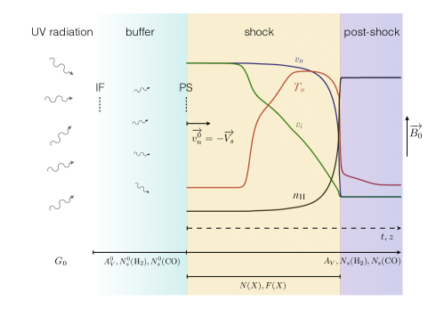
Figure 1: Schematic view of the shock model geometrical assumptions in the shock frame. The positions of the ionization front and of the pre-shock are indicated as IF and PS.

The model presented in this work is based on the Paris-Durham shock code (Flower & Pineau des Forêts 2003), a public numerical tool designed to compute the dynamical, thermal, and chemical evolution of interstellar matter in a steady-state plane-parallel shock wave. We further improve the version recently developed by Lesaffre et al. (2013), which is built to follow the effects of moderate ultraviolet irradiation, by including additional fundamental processes of PDR physics to study the propagation and chemistry of molecular shocks over a broad range of irradiation conditions.

2.1 Geometry and main parameters

A schematic view of the plane-parallel geometry adopted in the model is shown on Fig. 1. Following the prescription of Lesaffre et al. (2013), we assume that a plane-parallel shock wave propagates with a speed ${\bf V}_{\rm s}$ with respect to the pre-shock gas, in the direction perpendicular to the illuminated surface of the gas and to the ambient magnetic field ${\bf B_{0}}$. The shock wave is irradiated upstream by an isotropic flux of UV photons equal to the standard interstellar radiation field (Mathis et al. 1983) scaled with a parameter $G_{0}$. A plane-parallel layer of gas and dust (hereafter designated as the ”buffer”) is also assumed to stand upstream of the shock reducing the UV photon flux that reaches the pre-shock medium over a distance set by its visible extinction $A_{V}^{0}$ or equivalently its total hydrogen column density $N_{\rm H}^{0}$.

The last point of the buffer corresponds to the pre-shock medium and marks the origin of time $t$ and distance $z$ for the computation of the shock. The visible extinction $A_{V}$ and the self-shielding column densities of $\rm H_{2}$ and CO in the shock, $N_{s}({\rm H_{2}})$ and $N_{s}({\rm CO})$, are integrated over the entire structure, including the buffer, to account correctly for the total absorption of UV photons. However, the output column density $N({\rm X})$ and line flux $F({\rm X})$ of any species X shown throughout the paper are integrated over the shock only, ignoring both the buffer and post-shock medium. Details on the computation of the timescale $t_{\rm s}$ and size $z_{\rm s}$ of the shock are given in Sect. 3.5.

In practice, we first compute the radiative transfer and chemical and thermal structures of the buffer with the Paris-Durham shock code by following, in a Lagrangian frame, a fluid particle moving away from the ionization front at a small and constant velocity until it reaches the position PS (see Fig. 1) where it enters the shock. Using the physical properties of the pre-shock gas as initial conditions, we then run the code in its classical configuration and compute the time-dependent dynamical, chemical, and thermal evolution of matter in the shock.

The main parameters of the model and the range of values explored in this work are given in Table 1. Compared to Table 1 of Lesaffre et al. (2013), we removed $N_{s}^{0}({\rm H_{2}})$ and $N_{s}^{0}({\rm CO})$ from the list of parameters because those quantities, which correspond to the column densities of $\rm H_{2}$ and CO in the buffer layer, are now self-consistently calculated by the code when computing the properties of the pre-shock gas.

Table 1: Main parameters of the shock code, standard model, and range of values explored in this work.

name	standard	range	unit	definition
$n_{\rm H}$	$10^{4}$	$10^{2}$ $-$ $10^{5}$	cm-3	pre-shock proton densitya
$G_{0}$	1	0 $-$ $10^{4}$		radiation field scaling factorb
$A_{V}^{0}$	$10^{-2}$ & $10^{-1}$	$10^{-2}$ $-$ $10^{1}$		pre-shock visual extinction
$u_{\rm turb}$	1	$-$	km s-1	turbulent velocity
$\zeta_{{\rm H_{2}}}$	$3\times 10^{-17}$	$-$	s-1	$\rm H_{2}$ cosmic-ray ionization rate
$V_{\rm s}$	10	5 $-$ 25	km s-1	shock velocity
$b$	1	0.1 $-$ 10		magnetic parameterc

• (a) defined as ${n_{\rm H}}=n({\rm H})+2n({\rm H_{2}})$.
  (b) the scaling factor $G_{0}$ is applied to the standard ultraviolet radiation field of Mathis et al. (1983).
  (c) sets the initial transverse magnetic field $\frac{B_{0}}{1\mu{\rm G}}=b\times(\frac{{n_{\rm H}}}{1{\,{\rm cm}^{-3}}})^{0.5}$.

2.2 Grains and PAHs

As described in Appendix A, we assume that the grains at the ionization front (IF in Fig. 1) follow a power-law size distribution. Such distribution is subsequently modified in the buffer and in the shock as erosion, adsorption, and desorption processes take place. The initial range of sizes considered, the assumed mass densities of the grain cores and mantles, and the chemical composition of the cores are all given in Table 3. Conversely, we model PAHs as single particles of size 6.4 Å and chemical composition C₅₄H₁₈. To allow comparisons with the model developed by Lesaffre et al. (2013), a fixed abundance $n({\rm PAH})/{n_{\rm H}}=10^{-6}$ is adopted throughout the entire paper.

2.3 Ultraviolet continuum radiative transfer

The attenuation of the UV photons flux throughout the geometry shown in Fig. 1 is solved using a simplified model of radiative transfer. We only consider absorption and neglect all emission and diffusion processes by gas and dust. Under these approximations, the specific monochromatic intensity $I$ at a wavelength $\lambda$ propagating in the cloud satisfies a reduced radiative transfer equation

$${\rm cos}(\theta)\frac{\partial I(z,\theta,\lambda)}{\partial z}=-\kappa(z,\lambda)I(z,\theta,\lambda),$$ (1)

where $z$ is the distance to the border of the cloud, $\theta$ is the angle of the propagation direction (with respect to the direction perpendicular to the cloud surface), and $\kappa=\kappa_{D}+\kappa_{G}$ is the sum of the dust and gas absorption coefficients. Integrating this equation over the distance $z$ leads to a simple relation

$$I(z,\theta,\lambda)=I_{0}(\theta,\lambda)\,\,{\rm exp}\left[-\int_{0}^{z}\frac{\kappa(s,\lambda)}{{\rm cos}(\theta)}ds\right]$$ (2)

between $I$ and $I_{0}$, the specific monochromatic intensity at the border of the cloud. We define

$$\tau_{\lambda}=\int_{0}^{z}\frac{\kappa(s,\lambda)}{{\rm cos}(\theta)}ds$$ (3)

and

$$A_{\lambda}=2.5\,{\rm log}_{10}(e)\,\tau_{\lambda},$$ (4)

respectively, as the optical depth and the extinction along the direction $\theta$. The monochromatic mean intensity, averaged over all directions, can be written

$$J(z,\lambda)=\frac{1}{2}\int_{0}^{\pi/2}I(z,\theta,\lambda)\,{\rm sin}(\theta)\,d\theta$$ (5)

and the UV photon flux integrated between $\lambda_{\rm min}=911$ Å and $\lambda_{\rm max}=2400$ Å

$$F(z)=2\pi\int_{0}^{\pi/2}\int_{\lambda_{\rm min}}^{\lambda_{\rm max}}\frac{\lambda}{hc}I(z,\theta,\lambda)\,{\rm sin}(\theta)\,d\theta\,d\lambda.$$ (6)

Absorption of UV photons by grain particles is calculated considering grains with density $n_{g}$ and a single size $a_{g}$, where $n_{g}$ is derived from the size distribution while

$$a_{g}=\sqrt{\langle r_{m}^{2}\rangle}$$ (7)

is chosen as the size representative of the cross section of grains covered by ice mantles (see Appendix A). Within this framework, the dust attenuation coefficient at position $z$ is therefore

$$\kappa_{D}(z,\lambda)=\pi\,a_{g}^{2}(z)\,Q_{\rm abs}(a_{g},\lambda)\,n_{g},$$ (8)

where $Q_{\rm abs}(a_{g},\lambda)$ is the absorption coefficient of the grains. For simplicity, we adopt the absorption coefficients of spherical graphite grains of radius $a_{g}$ derived by Draine & Lee (1984) and Laor & Draine (1993).

The absorption of UV photons by the gas is finally taken into account considering only continuum processes, i.e. the photodissociation and photoionization of atoms and molecules. The gas attenuation coefficients are thus

$$\kappa_{G}(z,\lambda)=\sum_{i}\sigma({\rm X}_{i},\lambda)\,n({\rm X}_{i}),$$ (9)

where $\sigma({\rm X}_{i},\lambda)$ is the photodissociation or photoionization cross section of species ${\rm X}_{i}$. The code is written to potentially include all cross sections available in the Leiden database and recently updated by Heays et al. (2017). In this paper, however, and to reduce the complexity of the problem, $\kappa_{G}(z,\lambda)$ is computed including only the photoionization of C, S, C₂, CH, OH, and H₂O, and the photodissociation of C₂, C₃, CH, OH, and H₂O. We chose this approach to treat properly the ionization of the main atomic compounds and the destruction of several carbon and oxygen bearing species, which are discussed in Sect. 4. All the other photodestruction processes are implemented in the chemistry alone and not in the radiative transfer.

With these settings, the radiative transfer equation (Eq. 2) is solved along 20 directions spread between $\theta=0$ and $\theta=\pi/2$. The discretization leads to an error in the calculation of the UV photon flux of about 8% for an isotropic radiation field (at the ionization front) and of less than 10% deeper in the cloud. We present in Appendix B a detailed comparison between our approach and the predictions of the Meudon PDR code (Le Petit et al. 2006) for the same environment. With the grain parameters described in Appendix A, the prescriptions adopted in this work are able to capture the physical structure and chemical transitions obtained in state-of-the art PDR codes (Le Petit et al. 2006; Le Bourlot et al. 2012).

2.4 Photodestruction processes

Photodestruction of atoms and molecules can involve continuum processes, i.e. occur through the absorption of photons over a continuous range of energy, or line processes, i.e. occur through the absorption of photons in atomic or molecular lines at given wavelengths (e.g. van Dishoeck 1988; van Dishoeck et al. 2006). In this work we take advantage of the computation of the radiation field spectrum to perform detailed treatments of both processes.

Following the approach of the Meudon PDR code (Le Petit et al. 2006), the continuum absorption mechanisms are treated in two different ways. If the photodestruction cross section of a species ${\rm X}_{i}$ is known and included in the code, the corresponding photoreaction rate is computed by direct integration over the radiation field intensity

$$k_{\gamma}({\rm X}_{i},z)=2\pi\int_{0}^{\pi/2}\int_{\lambda_{\rm min}}^{\lambda_{\rm th}}\sigma({\rm X}_{i},\lambda)\,\frac{\lambda}{hc}I(z,\theta,\lambda)\,{\rm sin}(\theta)\,d\theta\,d\lambda,$$ (10)

where $\lambda_{\rm th}$ is the ionization or dissociation threshold (expressed in wavelength). If not, the photoreaction rate is calculated using the analytical fits provided by Heays et al. (2017). In PDR physics, it is customary to express such rates as functions of the visual extinction $A_{V}$ with the form

$$k_{\gamma}({\rm X}_{i},z)=G_{0}\,\alpha\,{\rm exp}(-\beta A_{V}),$$ (11)

where $\alpha$ and $\beta$ are constant coefficients. Such prescription, however, can only be applied if the visual extinction, used in this case as a proxy for the absorption of UV photons, has the same significance as the visual extinction deduced from the radiative transfer, or, in other words, if the underlying dust extinction curve used in Eq. 11 and that used in the radiative transfer are identical. To allow a coherent treatment of the photochemistry and the extinction based solely on the dust composition and size distribution chosen in input, we substitute relation 11 by a more versatile expression

$$k_{\gamma}({\rm X}_{i},z)=G_{0}\,\alpha\,\left(\frac{F(z)}{F_{\rm ISRF}}\right)^{\frac{\beta}{2.8}},$$ (12)

where $F_{\rm ISRF}$ is the UV photon flux associated with the isotropic standard interstellar radiation field (ISRF) for which the $\alpha$ and $\beta$ coefficients are computed, and the factor $2.8$ is deduced from a power-law fit of the photon flux $F(z)$ as a function of $A_{V}$ for $0\leqslant A_{V}\leqslant 3$ assuming a galactic extinction curve.

A different treatment is required for the photodissociations of $\rm H_{2}$ and CO that occur in lines and therefore involve self- and cross-shielding processes (Abgrall et al. 1992; Lee et al. 1996; Le Petit et al. 2002). In the previous version of the code, these aspects were taken into account using the analytical shielding expressions tabulated by Lee et al. (1996) and Draine & Bertoldi (1996) as functions of the column densities of $\rm H_{2}$ and CO at the current point (Lesaffre et al. 2013). To improve the treatment of the photodissociation of $\rm H_{2}$, we part from this approach and compute the absorption of UV photons by electronic lines of molecular hydrogen and the subsequent dissociation probabilities. This treatment is performed using the FGK approximation (Federman et al. 1979) and including all the UV lines of $\rm H_{2}$ in the Lyman and Werner bands. At each point $z$ the code computes the central optical depth of each of those lines by integrating the abundance of $\rm H_{2}$ towards the radiation source, taking into account the thermal broadening and microturbulent motions (set with a parameter $u_{\rm turb}$, see Table 1) in the Doppler spreading of the line profiles. These optical depths are then used to attenuate the radiation field at the line central wavelengths, hence reducing the $\rm H_{2}$ dissociation rate.

Admittedly, large velocity gradients such as those found in shock waves could have an impact on the computation of optical depths and therefore on the photodissociation rate of $\rm H_{2}$ (Monteiro et al. 1988). This effect is, however, not yet included in the model.

2.5 Chemical network

The treatment of chemistry is carried out starting with the network of Flower & Pineau des Forêts (2015). This network incorporates 139 species, including gas-phase and solid-phase compounds, and about a thousand reactions. Regarding gas-phase reactions, both the sulphur and nitrogen chemistries are modified to take into account the recent updates of the reaction rates introduced in Table D1 of Neufeld et al. (2015) and Tables B1-B3 of Le Gal et al. (2014). Regarding interactions with grains, we expand the network to model thermal desorption and photodesorption processes in addition to the sputtering, cosmic-ray and secondary photons desorption mechanisms already included in the previous versions.

Following Hollenbach et al. (2009), the thermal desorption rate per atom or molecule of a species ${\rm X}_{i}^{*}$ stuck on grain mantles is modelled as

$$k_{\rm thd}({\rm X}_{i}^{*},z)=1.6\times 10^{11}\sqrt{\frac{E_{i}}{k}\frac{m_{\rm H}}{m_{i}}}\,{\rm exp}\left(-\frac{E_{i}}{kT_{g}(z)}\right),$$ (13)

where $m_{i}$ is the mass of ${\rm X}_{i}^{*}$, $E_{i}$ its adsorption energy taken from Hasegawa & Herbst (1993) and Aikawa et al. (1996), and $T_{g}(z)$ is the grain temperature. The photodesorption rate of ${\rm X}_{i}^{*}$ is written

$$k_{\rm phd}({\rm X}_{i}^{*},z)=Y_{i}\,F(z)\,\pi\,\langle r_{m}^{2}\rangle\,n_{g}\,f_{i},$$ (14)

where $Y_{i}$ is the photodesorption yield set to $10^{-3}$ for all species (Hollenbach et al. 2009), and $f_{i}$ is the fraction of the surface adsorption sites occupied by ${\rm X}_{i}^{*}$.

The calculation of the desorption rates by interaction with secondary photons is finally modified to be coherent with the expression used for grain ionization. Adopting the formalism of Flower & Pineau des Forêts (2003), we model the secondary photon desorption rate of species ${\rm X}_{i}^{*}$ as

$$k_{\rm scd}({\rm X}_{i}^{*},z)=0.15\,\left[\zeta_{{\rm H_{2}}}n({\rm{\rm H_{2}}})+\zeta_{\rm H}n({\rm H})\right]\frac{n({\rm{\rm H_{2}}})}{n({\rm H})+n({\rm{\rm H_{2}}})}\,Y_{i}\,f_{i}.$$ (15)

The values $\zeta_{{\rm H_{2}}}$ and $\zeta_{\rm H}$ are the primary cosmic-ray ionization rates of $\rm H_{2}$ and H. $0.15\,\left[\zeta_{{\rm H_{2}}}n({\rm{\rm H_{2}}})+\zeta_{\rm H}n({\rm H})\right]\frac{n({\rm{\rm H_{2}}})}{n({\rm H})+n({\rm{\rm H_{2}}})}$ is thus the number of secondary UV photons produced per second and per unit volume through the excitation of the Rydberg states of $\rm H_{2}$ by cosmic-ray induced electrons.

Because our analysis is limited to low velocity shocks ($V_{S}\leqslant 25$ km s^-1) and low pre-shock densities (${n_{\rm H}}\leqslant 10^{5}$ $\,{\rm cm}^{-3}$), we neglect, throughout this paper, the effects of grain-grain interactions, such as shattering, vaporization, and coagulation (e.g. Jones et al. 1996). This approximation is supported by recent models of grain dynamics which show that the shattering and vaporization of large grains have a significant impact on the grain size distribution only for high velocity shocks ($V_{S}>20$ km s^-1) propagating in dense media (${n_{\rm H}}>10^{4}$ $\,{\rm cm}^{-3}$) (see Fig. 7 of Guillet et al. 2009 and Fig. 4 of Guillet et al. 2011). Similarly, the grain coagulation is found to marginally affect the grain size distribution in low density molecular shocks (see Fig. 14 of Guillet et al. 2011).

2.6 H₂ radiative pumping

Besides the thermal and chemical evolution of the gas, the code also computes the time-dependent populations of the rovibrational levels of $\rm H_{2}$ (Flower & Pineau des Forêts 2003). In addition to inelastic collisions with H, He, $\rm H_{2}$, and H⁺ and the probability of exciting $\rm H_{2}$ at formation on grain surfaces, which are two processes already taken into account, we include the excitation by radiative pumping of the electronic lines of molecular hydrogen followed by fluorescence.

The radiative pumping is computed following the approach used to estimate the self-shielding and photodissociation rate (see Sect. 2.4). At each time step, the absorption of UV photons by the discrete lines of the Lyman (${\rm B}^{1}\Sigma_{u}^{+}-{\rm X}^{1}\Sigma_{g}^{+}$) and Werner (${\rm C}^{1}\Pi_{u}-{\rm X}^{1}\Sigma_{g}^{+}$) band systems and the subsequent cascades in the rovibrational levels of the fundamental electronic state are calculated. The line opacities, which reduce the intensity of the radiation field capable of pumping the electronic states, are integrated over the column density $N_{s}({\rm H_{2}})$ (see Fig. 1) using the FGK approximation (Federman et al. 1979).

2.7 Dust charge and temperature

Grains are considered to be either neutral, negatively, or positively charged. As done for the radiative transfer, the abundances of these different states are computed assuming grains with a single size $a_{g}$. Photoelectric ejection, electron attachment, and charge exchange between ions and grains are modelled adopting the formalism of Bakes & Tielens (1994). The photoelectric ejection rate of a grain of charge $Z$ is thus written

$$k_{\rm phe}(Z,z)=\int_{\Omega}\int_{\lambda}Y_{\rm ion}(a_{g},Z)\,\pi\,a_{g}^{2}(z)\,Q_{\rm abs}(a_{g},\lambda)\,\frac{\lambda}{hc}I(z,\Omega,\lambda)d\Omega\,d\lambda,$$ (16)

where $Y_{\rm ion}(a_{g},Z)$ is the ionization yield, and the charge attachment rate

$$k_{\rm att}(Z,z)=n({\rm X_{i}})\left(\frac{8kT_{i}}{\pi m_{i}}\right)^{1/2}\pi a_{g}^{2}\tilde{J}\left(\tau=\frac{a_{g}kT_{i}}{Z({\rm X_{i}})^{2}},\nu=\frac{Ze}{Z({\rm X_{i}})}\right),$$ (17)

where $n({\rm X_{i}})$ and $Z({\rm X_{i}})$ are the abundance and charge of the colliding particle ${\rm X_{i}}$, and $T_{i}$ is the ion temperature. The function $\tilde{J}$ is described by Draine & Sutin (1987) and accounts for Coulomb interactions of the colliding system.

The heating rate of the gas induced by the photoelectric effect is modelled using the efficiencies deduced by Bakes & Tielens (1994) for very small graphitic grains and PAHs (Eqs. 42 and 43 of their paper).

At last, the temperature $T_{d}$ of grains of size $a_{g}$ is computed from the equilibrium between the radiative energy absorbed by the grain, the thermal exchange induced by collisions between grains and gas (at temperature $T_{n}$), and infrared radiative emission,

$$E_{\rm abs}+E_{\rm gg}=E_{\rm em},$$ (18)

where

$$E_{\rm abs}=\int_{\Omega}\int_{\lambda}\pi\,a_{g}^{2}(z)Q_{\rm abs}(a_{g},\lambda)I(z,\Omega,\lambda)d\Omega\,d\lambda,$$ (19)

$$E_{\rm gg}=3.5\times 10^{-34}\,\sqrt{T_{n}}\,(T_{n}-T_{d})\,n_{\rm H}^{2}/n_{g},$$ (20)

and

$$E_{\rm em}=\int_{\Omega}\int_{\lambda}\pi\,a_{g}^{2}(z)Q_{\rm abs}(a_{g},\lambda)B_{\lambda}(T_{d})d\Omega\,d\lambda,$$ (21)

assuming that grains radiate as black-bodies with an intensity equal to the Planck function $B_{\lambda}(T_{d})$. In the code, $T_{d}$ is computed at each time step by solving Eq. 18 using a Newton-Raphson scheme.

2.8 Cooling

Following Flower & Pineau des Forêts (2003) and Lesaffre et al. (2013), the cooling of the gas is computed taking into account the excitation of the fine structure lines and metastable lines of C, N, O, S, Si, C⁺, N⁺, O⁺, S⁺, and Si⁺, and the rovibrational lines of $\rm H_{2}$, OH, H₂O, NH₃, ¹²CO, and ¹³CO. The cooling resulting from the atomic lines and rovibrational lines of $\rm H_{2}$ is calculated in the optically thin limit. In the framework of a 1D plane-parallel geometry, this assumption is found to hold for the main coolant of the gas (namely $\rm H_{2}$, C⁺, and O) at a level better than a few percent. The cooling through the rovibrational lines of OH and NH₃ is calculated analytically using the prescription of Le Bourlot et al. (2002), while the cooling induced by the molecular lines of H₂O, ¹²CO, and ¹³CO is taken from the values tabulated by Neufeld & Kaufman (1993), which include opacity effects.

3 The models: C, C*, CJ, and J stationary shocks

The influence of the external UV field on the propagation and properties of interstellar shocks is studied through several grids of models $-$ 3120 runs in total $-$ covering a broad range of physical conditions. These include an initial pre-shock density varying between $10^{2}$ and $10^{5}$ $\,{\rm cm}^{-3}$, an ambient UV radiation field with a scaling factor $G_{0}$ between $0$ and $10^{4}$, and a total hydrogen column density in the buffer between $2\times 10^{19}$ and $2\times 10^{22}$ cm^-2 (see Table 1). For reasons we detail below (see Sect. 5.2), we limit our analysis to low velocity and moderately magnetized shocks, i.e. shocks with a speed comprised between 5 and 25 km s^-1 and a pre-shock transverse magnetic field parameterized by $b$ (see Table 1) varying between 0.1 and 10.

3.1 Pre-shock conditions

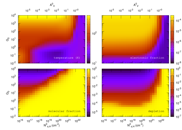
Figure 2: Temperature (top left), electronic fraction (i.e. $n(e)/{n_{\rm H}}$, top right), molecular fraction (i.e. $2n({\rm H_{2}})/{n_{\rm H}}$, bottom left), and depletion (bottom right) in the pre-shock medium as functions of $G_{0}$ and $N_{s,{\rm H}}^{0}$ (or $A^{0}_{V}$) for a density ${n_{\rm H}}=10^{4}$ $\,{\rm cm}^{-3}$. The depletion is computed as the fraction of the abundance of heavy elements locked up onto grain mantles.

The range of pre-shock conditions explored in this work are summarized in Fig. 2, which shows the temperature, electronic fraction, molecular fraction, and depletion of elements on grain surfaces in the pre-shock gas as functions of the input radiation field and size of the buffer. Since the amount of elements locked up onto grain surfaces in well-shielded environments is highly uncertain (Gibb et al. 2000), two formalisms are considered: if there is no radiation field ($G_{0}=0$), we switch off all adsorption and desorption processes for the computation of the pre-shock conditions and adopt the chemical composition of grain mantles given in Table 2 of Flower & Pineau des Forêts (2003); conversely, if a radiation field with any strength is illuminating the gas and dust (as in Fig. 2), both adsorption and desorption processes are included. We note that this last assumption may lead to strong depletion at low radiation fields (bottom right panel of Fig. 2), which may be unrealistic compared to observations.

Fig. 2 shows the well-known transition regions of PDRs discussed in many studies (i.e. Hollenbach & Tielens 1999; Röllig et al. 2007). Within the FGK approximation (see Sect. 2.6), the treatment of the radiative pumping of $\rm H_{2}$ rovibrational levels has a small influence on the general properties of the gas and on the pre-shock conditions shown in Fig. 2. The most noticeable impact arises at large radiation fields ($G_{0}\geqslant 10^{3}$) where the pre-shock temperature and electronic fraction increase by more than 10 % when the pumping is included. While inconsequential over a wide range of parameters, this process is however paramount for shocks propagating in hot and dense PDRs (i.e. $G_{0}=10^{4}$ and ${n_{\rm H}}=10^{5}$ $\,{\rm cm}^{-3}$) in which the UV pumping strongly limits the cooling efficiency of $\rm H_{2}$ and induces a raise of the pre-shock temperature (see Fig. 19 of Appendix D).

As shown in Fig. 2, the range of parameters chosen in this work allows us to explore shocks propagating in a wide variety of environments, spanning atomic to molecular gas, low and high ionization conditions, and cold and hot pre-shock medium (from $\sim 20$ K to $\sim 1000$ K). While extensive grids of shock models have been run over the entire parameter space, most of the analysis below is carried out varying one parameter at a time around two standard models defined as follows: ${n_{\rm H}}=10^{4}$ $\,{\rm cm}^{-3}$, $G_{0}=1$, $V_{S}=10$ km s^-1, $b=1$, and $A_{V}^{0}=10^{-2}$ or $10^{-1}$. In order to highlight the impacts of the UV radiation field on the dynamics of the gas, a buffer visual extinction $A_{V}^{0}=10^{-2}$ is assumed throughout all Sect. 3. Conversely, the predictions on atomic and molecular emission presented in Sect. 4 are obtained assuming $A_{V}^{0}=10^{-1}$. Such choice of standard models not only opens the exploration of all the conditions shown in Fig. 2 with a limited number of runs but is also found to be sufficient to present most of our results on the physics of irradiated shocks in a synthetic manner. More exhaustive results are given in Appendix D where we lay out additional figures and predictions in a blooming potpourri.

3.2 Stationary magnetized molecular shocks

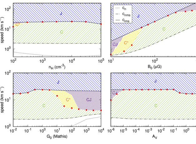
Figure 3: Neutral sound speed (dotted) and neutral (dot-dashed) and ion (solid) magnetosonic speeds as functions of the density (upper left), transverse magnetic field intensity (upper right), UV radiation field intensity (lower left), and visual extinction (lower right). All the non-varying parameters are set to their standard values (see Table 1), and the standard value of the buffer visual extinction is set to $A_{V}^{0}=10^{-2}$. The critical velocities above which C-type shocks cannot exist are shown with red points, while coloured areas highlight the range of velocities at which C- (green), C*- (yellow), CJ- (violet), and J-type (blue) shocks develop.

We recall that the standard model adopted in this section is defined by a buffer visual extinction $A_{V}^{0}=10^{-2}$. The physics of magnetized molecular shocks and the steady-state solutions allowed to propagate in the interstellar medium have been described in many studies (e.g. Mullan 1971; Draine 1980; Kennel et al. 1990; Dopita & Sutherland 2003). As prescribed by the Paris-Durham code, we limit our study to stationary plane-parallel shock waves where the magnetic field is assumed to be transverse to the direction of propagation. It follows that the influence of UV photons on time-dependent shocks (Chièze et al. 1998; Lesaffre et al. 2004) and on slow or intermediate steady-state shocks (Draine & McKee 1993; Lehmann & Wardle 2016) are not addressed in this work.

A shock is a pressure-driven instability of fluid dynamics in which the kinetic energy of the flow is transferred from large scales to small scales where it dissipates primarily into heat. At steady-state, a shock structure connects two thermodynamical equilibrium points: the upstream unstable state and downstream stable state. The nature of the instability, the scales involved, and the forces at play in the evolution of the fluid between these two points depend on the velocity of the flow compared to its characteristic wave speeds. Although the expressions of those speeds are different depending on the physical properties of the gas, it is customary to discuss the physics of shocks in terms of the wave speeds derived for an isothermal magnetohydrodynamic fluid in the limit of weak and strong coupling between ionized and neutral species, i.e. the sound speeds and magnetosonic speeds in the ions ($c_{\rm i}$ and $c_{\rm ims}$) and in the neutrals ($c_{\rm n}$ and $c_{\rm nms}$)

$$c_{\rm i}=\left(\gamma_{i}P_{i}/\rho_{i}\right)^{1/2},$$ (22)

$$c_{\rm n}=\left(\gamma_{n}P_{n}/\rho_{n}\right)^{1/2},$$ (23)

$$c_{\rm ims}=\left(c_{\rm i}^{2}+B^{2}/4\pi\rho_{i}\right)^{1/2},\quad{\rm and}$$ (24)

$$c_{\rm nms}=\left(c_{\rm n}^{2}+B^{2}/4\pi\rho_{n}\right)^{1/2},$$ (25)

where $\gamma_{i}$, $\gamma_{n}$, $P_{i}$, $P_{n}$, $\rho_{i}$, and $\rho_{n}$ are the heat capacity ratio, pressure, and mass density of the ions and the neutrals and $B$ is the strength of the magnetic field. As we explain below (see Sect. 3.3.3), we assume that all grains are coupled with the magnetic field: it follows that $\rho_{i}$ not only includes the mass density of ionized species but also that of dust particles. Interstellar shocks occur when the upstream flow is dynamically unstable, which happens when $V_{S}\geqslant c_{\rm n}$ (resp. $c_{\rm nms})$ in the limit of weak (resp. strong) coupling between ions and neutrals.

Assuming a fixed ionization fraction, the nature of a shock can be understood by solely discussing the impact of the magnetic field and gas cooling.

In very weak magnetic field environments, ions and neutrals are fully coupled with each other. In the frame of the shock, both fluids are decelerated through the combined actions of viscous stresses and the thermal pressure gradient induced by viscous heating. The gas quickly jumps from a supersonic to a subsonic regime, with respect to the neutral sound speed, over a distance of about a few mean free paths. The resulting structure is referred to as a J-type shock. Without magnetic field, the gas pressure of the post-shock flow is only thermal, which implies that the downstream fluid is subsonic. If a magnetic field is present, magnetic pressure increases in the post-shock. In this case, the final velocity of the flow may be supersonic if the magnetic pressure is large enough to stabilize the downstream flow.

When the magnetic field is sufficiently strong such that $c_{\rm ims}>V_{S}$, a magnetic precursor can develop: the Lorentz force decelerates the ions which decouple from the neutrals in the upstream flow. In turn, this decoupling induces a drag force that slows down the neutral fluid. If the coupling between ions and neutrals is weak, the resulting effect is too small to smooth the neutral velocity gradient: the viscous stresses and thermal pressure gradient remain the dominant forces involved in the motion of the neutrals. Two characteristic lengths therefore appear: the magnetic precursor scale (Draine 1980) over which the ions decelerate continuously, and the viscous length where the neutrals velocity jumps. Such a structure is called a CJ-type shock. While the neutral fluid necessarily becomes subsonic at the jump, the downstream flow may be supersonic (for reasons given above). In this case, the neutral fluid crosses the sonic speed twice, at the jump position and somewhere along the downstream trajectory.

Increasing the magnetic field enlarges the size of the magnetic precursor. The drag force applies for a longer time, smoothing the neutral velocity gradient and thermal pressure gradient, thus reducing the strength of viscous stresses which may become negligible over the entire trajectory. When this happens, the thermal pressure gradient and the ion-neutral friction slow down the neutrals continuously to the downstream point. Those kinds of shocks are separated into two classes. If the neutral fluid becomes subsonic along its trajectory, the structure is referred to as a C*-type shock, if not as a C-type shock. It follows that the downstream flow of a C-type shock is necessarily supersonic. It is worth noting that the differentiation between C*- and C-type shocks is one of semantics and numerics only. These two types of shocks formally and physically correspond to the same kind of structure with similar thermochemical evolutions (see Sect. 3.4).

The impact of the cooling described by Chernoff (1987) can be understood starting with a CJ-type shock. Increasing the cooling in this situation reduces the thermal pressure gradient and neutral velocity Laplacian, hence the strength of the viscous stresses. As in the previous case, if the viscous forces become small enough compared to the drag force and thermal pressure gradient, either a C*-type or a C-type structure develops.

The nature of an interstellar shock is therefore the result of a subtle interplay between the strength of the magnetic field and the ionization degree $-$ which control the size of the magnetic precursor and its capacity to slow down and heat the neutrals $-$ and the cooling rate. In practice single-fluid J-type shocks or bi-fluid C-type shocks are computed using a forward integration technique and starting from the pre-shock conditions (e.g. Flower & Pineau des Forêts 2015). Since this method is numerically unstable as soon as the neutral gas become subsonic, a more sophisticated algorithm is used to compute CJ-type and C*-type shocks. This algorithm, fully described in Appendix C, is based on the works of Chernoff (1987) and Roberge & Draine (1990) and combines forward integration techniques with shooting methods.

3.3 Existence of J-, CJ-, C*-, and C-type shocks

The characteristic speeds $c_{\rm n}$, $c_{\rm ims}$, and $c_{\rm nms}$ computed in the pre-shock fluid and the domains of existence of the different kinds of stationary shocks are shown in Fig. 3 as functions of the pre-shock density, magnetic field, and irradiation conditions. Each parameter is explored around the standard model for a buffer visual extinction $A_{V}^{0}=0.01$ (see Table. 1).

3.3.1 Critical speeds

The minimal speed required for a shock to propagate is a problem of non-ideal magnetohydrodynamic. In the limit of low coupling between ions and neutrals, a shock develops if the perturbation applied to the medium travels faster than the neutral sound speed. Conversely, in the limit of strong coupling, a shock exists only if the perturbation travels faster than the neutral magnetosonic speed. While the intermediate case has been treated in several numerical studies (e.g. Balsara 1996), no analytical formula has ever been derived. To simplify, we identify in Fig. 3 the neutral magnetosonic speed $c_{\rm nms}$ as the minimal speed required to induce a shock. We do so because we found that C-type shocks below this limit ($\sim$$2$ km s^-1 for the standard model) induce a relative velocity difference between the upstream and downstream flows smaller than 10%. Above this limit, the parameter space shown in Fig. 3 is divided in four different regions which set the domains of existence of J-, CJ-, C*-, and C-type shocks.

The limit between J-type and other kinds of molecular shocks is given by the ions magnetosonic speed, hence by the strength of the magnetic field and the mass density of the ionized flow in the pre-shock medium (Eq. 24). Assuming that all grains – including the neutrals – contribute to the inertia of the charged fluid (see Guillet et al. 2007; Lesaffre et al. 2013, and Sect. 3.3.3), the mass density of the ionized flow is dominated by the grains. With an initial transverse magnetic field $B_{0}$ proportional to $\sqrt{{n_{\rm H}}}$ (see Table 1), $c_{\rm ims}$ therefore linearly depends on $B_{0}$, does not depend on the gas density, and softly depends on the dust-to-gas mass ratio. Without depletion, i.e. at large radiation fields or weak extinctions (bottom panels of Fig. 2), the mass of grains lies in the cores which is set by their composition and grain size distribution (see Table 3 and Appendix A). Conversely, if the depletion becomes important, the mantles contribute to the grain mass; in the limit of high depletion, i.e. at low radiation fields or large extinctions, the dust-to-gas mass ratio is increased by a factor of two and the ion magnetosonic speed is divided by a factor 1.4.

The range of existence of C-, C*-, and CJ-type shocks below the ions magnetosonic speed can be explained in the light of the driving mechanisms of molecular shocks described in Sect. 3.2. The impact of the radiation field on a C-type shock is understood by two main processes: the enhancement of the photoionization mechanisms and the increase of the photodissociation of $\rm H_{2}$. Indeed, as the electronic fraction increases, so does the coupling between the ions and the neutrals: the size of the shock therefore decreases and the compressive heating rate increases. Concurrently, the diminution of both the self-shielding and the abundance of $\rm H_{2}$ strongly reduces the cooling rate of the gas. If the cooling is insufficient to prevent the neutrals from crossing the sound speed, the structure becomes a C* shock. If the cooling is even lower, i.e. too low to repress the impact of viscous stresses, the structure becomes a CJ shock.

The role of the magnetic field is also straightforward. Low magnetic field intensities reduce the size of the magnetic precursor, hence the size of the shock, favouring the existence of C* and CJ shocks (see Sect. 3.2). Conversely, large magnetic field intensities increase the ions magnetosonic speed, hence the maximal velocity for which a magnetic precursor can develop. When $c_{\rm ims}$ is larger than the critical speed required to dissociate $\rm H_{2}$ by collisions (Le Bourlot et al. 2002), a domain of existence of CJ shocks appears (top right panel of Fig. 3).

3.3.2 Influence of the UV field

Fig. 3 shows that the structure of interstellar stationary shocks is mostly governed by the intensity of the magnetic field and strength of the UV radiation field. The magnetic field tunes the magnitude of the coupling between ions and neutrals and therefore controls the range of velocities over which a shock can exist and a magnetic precursor can develop. Once those limits are set, the radiation field becomes the most decisive quantity: its impact on the ionization fraction and the cooling efficiency (magnified by the pumping of $\rm H_{2}$) determines the range of existence of C, C*, and CJ shocks.

Most shocks propagating in dense or low-illuminated environments (${n_{\rm H}}\geqslant 10^{4}$ $\,{\rm cm}^{-3}$ or $G_{0}\leqslant 1$) appear to be either J or C. This ceases to be true, however, in more diffuse or illuminated media (see Figs. 3 and 18) where the radiation field drastically reduces the domain of existence of C-type shocks in favour of C* and CJ-type structures. As a rule of thumb we find that those kinds of shocks become dominant as soon as

$$G_{0}>20\times\left(\frac{{n_{\rm H}}}{10^{4}\,\,{\,{\rm cm}^{-3}}}\right)^{1/2}.$$ (26)

It follows that only low velocity C-type shocks ($V_{S}\leqslant 5$ km s^-1) can propagate in prototypical PDR (${n_{\rm H}}\sim 10^{4}$, $G_{0}\sim 100$) or in very diffuse clouds (${n_{\rm H}}\sim 30$ $\,{\rm cm}^{-3}$, $G_{0}\sim 1$). This limit on the maximal velocity of C-type shocks is in agreement with the work of Melnick & Kaufman (2015) who found similar breakdown velocities in irradiated environments.

3.3.3 Influence of grains and PAHs

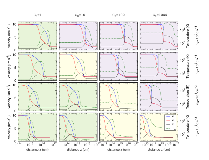
Figure 4: Profiles of the neutral sound speed (solid black), velocity of the neutrals (solid blue) and that of the ions (solid red) in the frame of the shock, and temperature of the neutrals (dot-dashed green) computed in stationary shocks propagating in media with different densities and radiation field intensities. All the other parameters are set to their standard values (see Table 1), and the standard value of the buffer visual extinction is set to $A_{V}^{0}=10^{-2}$. C-type, C*-type, and CJ-type shocks are highlighted in green, yellow, and violet, respectively.

The cold neutral medium is a partially ionized environment with a very low ionization fraction. Its elemental composition in the solar neighbourhood implies that the fraction of mass contained in gas-phase ionized species is below $3\times 10^{-3}$ for diffuse and transluscent clouds and quickly drops in dark clouds. With a dust-to-gas mass ratio of about 1% and efficient ionization and recombination processes, charged dust grains are thus a dominant contributor to the inertia of the ionized flow, and therefore strongly influence its dynamics.

The impact of dust on magnetized shocks has been the subject of many studies that have successively described the effects of the dust decoupling (e.g. Ciolek & Roberge 2002; Ciolek et al. 2004), their size distribution (e.g. Chapman & Wardle 2006; Guillet et al. 2009), and the fluctuation of their charge (Guillet et al. 2007) on the structure of the shock. Two results are of particular interest in this paper. Firstly, as the ionization and recombination of grains is fast, the charge of grains rapidly fluctuates. In particular, the survival timescale of a neutral grain is found to be very small compared to its dynamical timescale (Guillet 2008), i.e. the time it needs to reach the neutral velocity. This result holds for all grain sizes and all irradiation conditions. It follows that, for a given size of grains, both neutral and charged grains can be considered as a single fluid. Secondly, whether this fluid is coupled with the neutral flow or with the ionized flow solely depends on the Hall factor $\Gamma,$ which measures the ratio of the grain drag to the grain gyration timescales and depends on the grain elastic cross section $\sigma$, grain charge $q$, strength of the magnetic field $B$, mass density of the neutrals $\rho_{n}$, and velocity drift between grains and neutrals $\delta v$ as (Guillet et al. 2007, Eqs. 9 to 11)

$$\Gamma=\frac{\tau_{\rm drag}}{\tau_{\rm gyr}}\propto\frac{|q|B}{\rho_{n}\langle\sigma\delta v\rangle}.$$ (27)

The results shown here (including Fig. 3) are obtained adopting a PAH relative abundance of $\sim 10^{-6}$ and assuming that all grains are coupled to the magnetic field, i.e. $\Gamma>1$. Large grains in irradiated environments are expected to be multiply charged (e.g. Draine 2002). Because the Hall factor is inversely proportional to the square of the grain size, we estimate that this assumption is always valid for small grains ($a\leqslant 0.1$ $\mu$m) and holds for large grains as long as $G_{0}/{n_{\rm H}}\geqslant 10^{-4}$ cm³ and $b\geqslant 1$. In turn, it most probably fails in dense and dark environments ($G_{0}/{n_{\rm H}}\leqslant 10^{-5}$ cm³) or in media with a very low magnetic field ($b\sim 0.1$), where the Hall factor computed for grains larger than 0.2 $\mu$m falls below unity, which means that a fraction of the dust mass is coupled to the neutral fluid (Guillet et al. 2007). The main impact of PAHs is to reduce the abundance of electrons in the gas phase. In irradiated environments (resp. dark clouds), where grains are dominantly positive (resp. negative), PAHs therefore lead to an increase (resp. decrease) of the Hall factor. The rather large value of PAHs abundance adopted in this work therefore strengthens our hypothesis on the coupling between grains and the magnetic field in irradiated media but weakens it in dark environments.

As a whole, the outcome of this assumption ($\Gamma>1$) is a minimization of the ions magnetosonic velocity. This, in turn, reduces the range of existence of C, C*, and CJ shocks. In dark clouds with classical magnetization ($b=1$) for instance, where it could be debated, we find that these kinds of shocks propagate at velocities necessarily smaller than $\sim 25$ km s^-1 (see Fig. 18 of Appendix D); this value is significantly lower than the 40 km s^-1 derived in most of the previous studies (e.g. Kaufman & Neufeld 1996; Flower & Pineau des Forêts 2003, 2010; Melnick & Kaufman 2015) and also arguable. All these results show that a detailed treatment of grains and PAHs can be critical for the nature of interstellar shocks. For the sake of simplicity, we adopt a formalism which works over most of the parameter domain and extend it to environments where it may not be justified. An accurate treatment would allow us to study magnetized shocks in dark environments at velocities larger than the maximal value we infer. In practice, such a study requires us to adopt a multi-fluid approach to treat each size of grains as a separate flow with its own momentum and thermodynamical evolution (Ciolek & Roberge 2002; Chapman & Wardle 2006; Guillet et al. 2007). This is beyond the scope of this paper.

3.4 Shock profiles and energetics

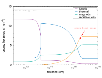
Figure 5: Kinetic, magnetic, and thermal energy fluxes compared to the integrated radiative loss in a CJ-type shock propagating at 10 km s^-1 in a medium of density $10^{4}$ $\,{\rm cm}^{-3}$ and illuminated by a strong radiation field $G_{0}=10^{4}$. All the other parameters are set to their standard values (see Table 1), and the standard value of the buffer visual extinction is set to $A_{V}^{0}=10^{-2}$. The light grey line corresponds to the total conserved energy flux. The red point highlights the criterion used to separate the shock from the post-shock region (Eq. 29).

The main physical properties of molecular shocks are shown in Fig. 4, which shows, in the frame of the shock, the ion and neutral velocity profiles and the neutral temperature profiles computed in different environments for shocks propagating at 10 km s^-1. Starting from the upstream supersonic state, a gas cell is progressively slowed down, compressed, heated up through compression, ion-neutral friction and viscosity, and eventually cooled down through line emission. The thermodynamical path followed by the cell and the final state reached downstream are simply the outcome of the mandatory conversion of the initial kinetic energy into magnetic and thermal energies and radiative losses (see Fig. 5).

In weakly magnetized J-type shocks with large compression ratios, the maximum temperature reached by the gas reduces to a simple analytical formula (Lesaffre et al. 2013)

$$T_{\rm max}=53\,\,(V_{S}/1{\,{\rm km}\,{\rm s}^{-1}})^{2}\,\,{\rm K},$$ (28)

which gives 5300 K for a shock at 10 km s^-1. This estimation corresponds to the extreme case where most of the initial kinetic energy is adiabatically converted into thermal energy at the shock front. In magnetized shocks or C-type shocks, part of the kinetic energy is used to compress the magnetic field, hence increase the magnetic pressure. The rest of the initial energy is converted into heat over a characteristic length controlled by both the size of the magnetic precursor and the cooling rate (see Sect. 3.2). The maximum temperature of those shocks is thus necessarily smaller than that obtained in the adiabatic case and decreases with the strength of the magnetic field and strength of the cooling. Such a behaviour has been abundantly confirmed with models of low radiation field environments or in dark clouds, where the temperature profiles of C-type shocks are found to be considerably smoother and broader than the equivalent profiles obtained in weakly magnetized J-type shocks with the same velocities (e.g. Flower 2010; Flower & Pineau des Forêts 2013; Lesaffre et al. 2013; Melnick & Kaufman 2015). For instance, these authors report typical maximal temperatures of 1000 K for 10 km s^-1 C-type shocks, a value five times lower than that found in the weakly magnetized adiabatic case.

The impact of an external UV radiation field can be understood in this framework. Increasing the radiation field increases the ionization fraction of the pre-shock medium, hence the strength of the coupling between the neutrals and the ions. As the magnetic precursor shrinks, the kinetic energy is converted into heat over a smaller distance, which leads to a larger maximal temperature of C-type shocks (see Fig. 4, Fig. 19 of Appendix D and Fig. 2 of Melnick & Kaufman 2015) that eventually become C*-type shocks. As shown in Fig. 19 of Appendix D, this effect is moderate and appears to be stronger for low velocity shocks and low density media. In particular, the thermodynamical profiles of C-type and C*-type shocks are found to be very similar and to differ only by their size and the fact that C*-type shocks are partly subsonic. This whole picture is, however, strongly modified at large radiation fields, when the flux of UV photons is strong enough to photodissociate $\rm H_{2}$. The reduction of the cooling rate of the gas leads to larger temperatures and eventually induces an adiabatic jump along the trajectory (CJ-type shock). As the radiation field increases, the jump arises sooner, instantly converting a large fraction of the kinetic energy into heat and magnetic compression. Depending on the velocity and the environment considered, the maximal temperature of CJ-type shocks can be two to ten times larger than that obtained in C-type shocks and persist over a large tail set by the long cooling timescale of the gas (see Fig 19).

3.5 Shock size and timescale

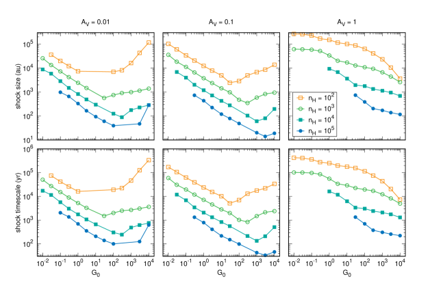
Figure 6: Shock sizes (top panels) and timescales (bottom panels) as functions of the UV radiation field and different visual extinction $A_{V}$ computed for shocks propagating at 10 km s^-1 in media of densities of $10^{2}$ (empty squares), $10^{3}$ (empty circles), $10^{4}$ (filled squares), and $10^{5}$ (filled circles) $\,{\rm cm}^{-3}$. The non-varying parameters are set to their standard values (see Table 1). J-type shocks propagating in dense and weakly irradiated clouds are deliberately removed from the figure (see main text), hence the missing points on the left side of each panel.

The determination of the shock size and timescale, i.e. the limit marking the beginning of the post-shock medium (see Fig. 1), is an important issue that is not only useful to interpret the physics of the shock but can also have a strong influence on the output quantities predicted by the models. Indeed, as shown for instance by Gusdorf et al. (2008a), Leurini et al. (2014), and Lehmann (2017), the inclusion of the post-shock gas (see Fig. 1) can modify by orders of magnitude the column densities of numerous species, and hence have a strong impact for the comparison with observations. Several definitions have been proposed so far, including criteria on the abundance profiles, temperature profile, or ion-neutral coupling length (Draine 1980; Wardle 1999; Lesaffre et al. 2013; Melnick & Kaufman 2015; Lehmann & Wardle 2016). Unfortunately, while these propositions may be useful to study a specific problem, they do not provide a reliable definition for comparison of shock length in different models and they cannot be applied indifferently to all kinds of shocks. In addition, any criterion based on the sole comparison of pre-shock and post-shock properties is bound to fail when strong external radiation fields are considered and if the post-shock medium conditions are nowhere near those of the pre-shock.

To overcome these issues, we adopt a definition of the shock size based on energetic considerations. As illustrated in Fig. 5, a stationary shock propagating in the interstellar medium is a structure in which the mechanical energy flux is progressively converted into magnetic and thermal energy fluxes and is partially radiated away through line emission. The transition between the shock and the post-shock medium can therefore be designated as the point at which most of the radiation induced by the shock has been emitted. In the following, we thus define the shock size $z_{s}$ as the distance verifying

$$\frac{\Upsilon(z)-\Upsilon(0)}{\Upsilon(\infty)-\Upsilon(0)}\geqslant 95\%,$$ (29)

where

$$\Upsilon(z)=\mathscr{F}_{\rm K}(z)+\mathscr{F}_{\rm B}(z)+\mathscr{F}_{\rm T}(z)$$ (30)

is the sum of the kinetic,

$$\mathscr{F}_{\rm K}(z)=\frac{1}{2}\left(\rho_{n}v_{n}^{3}+\rho_{i}v_{i}^{3}\right),$$ (31)

magnetic,

$$\mathscr{F}_{\rm B}(z)=\frac{B_{0}^{2}}{4\pi}\,\frac{V_{S}^{2}}{v_{i}},$$ (32)

and thermal,

$$\mathscr{F}_{\rm T}(z)=\frac{5}{2}k_{B}\left(\rho_{n}v_{n}T_{n}/\mu_{n}+\rho_{i}v_{i}T_{i}/\mu_{i}\right),$$ (33)

energy fluxes, and $\mu_{n}$ and $\mu_{i}$ are the mean molecular masses of the neutrals and of the ions. The shock timescale is then set as $t_{s}=t(z_{s})$, i.e. as the time required for a fluid particle to reach $z_{s}$. Because they are built on a conservative quantity, these definitions have the advantage of capturing key aspects of shock physics. Moreover they offer a more universal criterion that can be applied to any kind of structures, including C-, C*-, CJ-, or J-type shocks, propagating in dark or highly illuminated environments. An example of this criterion applied to an irradiated molecular shock is shown in Fig. 5.

The values of $z_{s}$ and $t_{s}$ obtained for a 10 km s^-1 shock propagating in various environments are shown in Fig. 6. To simplify, we deliberately remove from Fig. 6 the models at low radiation fields and large densities that correspond to J-type shocks propagating in a medium in which all the heavy elements are stuck onto grains. Indeed, while academically interesting, these models may be unrealistic for the study of dense and dark clouds, for which standard models usually assume a substantial fraction of heavy elements in the gas phase (e.g. Flower & Pineau des Forêts 2003; Gusdorf et al. 2008a, b; Guillet et al. 2009; Flower & Pineau des Forêts 2010; Anderl et al. 2013). Because the dark clouds are not the subject of this paper, these models are not studied.

Each panel of Fig. 6 can be separated in two regions depending on $G_{0}$ where the size and timescale of the shock either decrease or increase as functions of the strength of the UV field. (1) The first region, at low radiation field intensity, corresponds to the domain of existence of C-type and C*-type shocks. In this domain, the shock size is mainly given by the length of the magnetic precursor, which is inversely proportional to the electron density (see Eq. 36.44 of Draine 2011). If the UV photons are the main ionization source of the gas, i.e. at low extinction, it is easy to show that the electron density writes $n_{e}\propto(G_{0}{n_{\rm H}})^{1/2}$: the shock size is therefore proportional to $G_{0}^{-1/2}{n_{\rm H}}^{-1/2}$ as observed on the left and middle panels of Fig. 6. Conversely, if the UV photons are a secondary ionization process, i.e. at high extinction, the dependance on $G_{0}$ is progressively lost and the size of the shock becomes simply proportional to ${n_{\rm H}}^{-1/2}$ as confirmed on the right panels of Fig. 6. (2) The second region, where the size of the shock increases with the strength of the UV field, corresponds to the domain of existence of CJ-type shocks. In this domain, the ionization fraction has reached a maximum and the shock size is given by the large temperature tail induced by a reduced cooling efficiency due to the photodissociation of $\rm H_{2}$. If $\rm H_{2}$ is the major coolant of the gas, the shock size is inversely proportional to $n({\rm H_{2}})$, thus directly proportional to $G_{0}$ ; if $\rm H_{2}$ is a secondary coolant, the dependence of $z_{s}$ on $G_{0}$ is weak or lost. All these cases can be identified in the left and middle panels of Fig. 6.

Overall, Fig. 6 shows that the shock sizes and timescales cover a broad range of values, spread over three orders of magnitude, depending on the medium in which they propagate. Interestingly, if J-type shocks are removed from the analysis, the size of interstellar shocks appears to be weakly dependent on the shock velocity. Exploring the entire grid of models shows that similar sizes are found for $V_{S}$ varying between 5 and 20 km s^-1, except at very low radiation fields ($G_{0}/{n_{\rm H}}\sim 10^{-5}$ cm³) where sizes differ by a factor of four and at large radiation fields ($G_{0}/{n_{\rm H}}\geqslant 10^{-1}$ cm³) where they differ by a factor of three.

The crossing time represented in the bottom panels of Fig. 6 can be interpreted as the time required for the shock to reach its steady-state configuration (Chièze et al. 1998; Lesaffre et al. 2004). Scaling almost exactly as the shock size, this critical dynamical timescale is found to strongly depend on the medium considered, varying from a few hundred years in dense and moderately irradiated environments to a few tens of thousand years in diffuse gas. In most cases, these values are considerably smaller than the turnover timescales of the corresponding environment, suggesting that steady-state shocks are relevant structures for the study of interstellar medium. This is true, in particular, for diffuse and dense environments where the linewidth-size relation leads to dynamical timescales 100 times larger than the shock crossing time (e.g. Hennebelle & Falgarone 2012). This conclusion weakens, however, in outflows and jets (e.g. Gusdorf et al. 2008b) and in dense PDRs in which the photoevaporation timescale becomes comparable or smaller than the shock crossing time (Störzer & Hollenbach 1998). Comparing the results of Fig. 6 to the propagation timescale of ionization fronts (Gorti & Hollenbach 2002) shows that shocks can no longer be considered at steady state as soon as ${n_{\rm H}}\geqslant 10^{5}$ $\,{\rm cm}^{-3}$, $G_{0}\geqslant 10^{3}$ and $A_{V}\leqslant 10^{-2}$, i.e. at the border of our grid of models.

4 Molecules in irradiated shocks

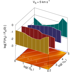
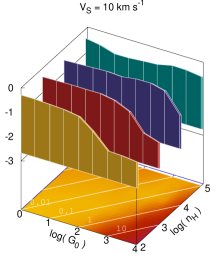
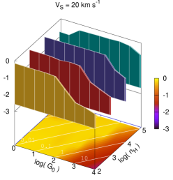
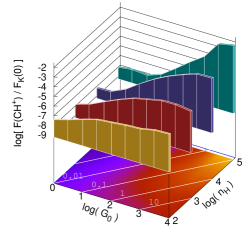
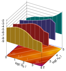
Figure 7: Total fluxes of $\rm H_{2}$ rovibrational lines (top panels) and $\rm CH^{+}$ rotational lines (bottom panels, summed up to the $J=10\rightarrow 9$ transition) emerging from shocks propagating at 5 (left panels), 10 (middle panels), and 20 (right panels) km s^-1 in different environments, for a buffer visual extinction $A_{V}^{0}=0.1$. The non-varying parameters are set to their standard values (see Table 1). All fluxes are normalized to the input kinetic energy flux of the shock $\mathscr{F}_{\rm K}(0)=\frac{1}{2}\rho V_{S}^{3}$. The results are displayed simultaneously as colour maps and fence plots at fixed densities of $10^{2}$ (yellow), $10^{3}$ (red), $10^{4}$ (blue), and $10^{5}$ (green) $\,{\rm cm}^{-3}$. White lines on the colour maps indicate contours of constant $G_{0}/{n_{\rm H}}$ ratio.

We recall that the standard model adopted in this section is defined by a buffer visual extinction $A_{V}^{0}=10^{-1}$. External sources of UV radiation fields necessarily exert a major impact on the formation and excitation of molecules in space. In irradiated shocks, the role of UV photons extends far beyond the mere ionization and dissociation processes: the combined effects of radiative and mechanical energies modify the structure of shocks, leading to specific chemical and radiative tracers. To analyse such effects, the line emission of molecular shocks are derived using two different approaches depending on the molecule considered. For $\rm H_{2}$, whose level populations are self-consistently computed by the code, line emissions are calculated in the optically thin limit by summing local emissivities. The level populations of other species are computed at statistical equilibrium and their line emissions are obtained by postprocessing the output of the shock model with the Large Velocity Gradient (LVG) code of Gusdorf et al. (2008a) slightly modified to take into account self-absorption in the line radiative transfer. In all cases, both intensities and column densities are computed over the shock only, i.e. without the contribution of the post-shock region identified through Eq. 29.

To discuss the results in light of a global energetic budget, this section addresses the following questions. What fraction of the input kinetic energy flux is radiated away through all the transitions of a given molecular species ? How is this total intensity spread in different lines ? As a first application, we focus on predictions regarding two important species: $\rm H_{2}$, whose rovibrational structure already observed in many galactic sources (e.g. Giannini et al. 2004; Gillmon et al. 2006; Neufeld et al. 2009; Habart et al. 2011) will soon be unveiled in extragalactic environments with the James Webb Space Telescope (JWST), and $\rm CH^{+}$, whose recent detection in emission in starburst galaxies at high redshift ($z\sim 2-3$) with ALMA may be to date the strongest signature of the combined effect of mechanical and radiative energy on interstellar chemistry (Falgarone et al. 2017). While other species are briefly discussed in Sect. 4.3, we defer detailed presentations of the impact of irradiated shocks on the rest of the chemistry to future papers, as motivated by emerging observational needs.

4.1 H₂

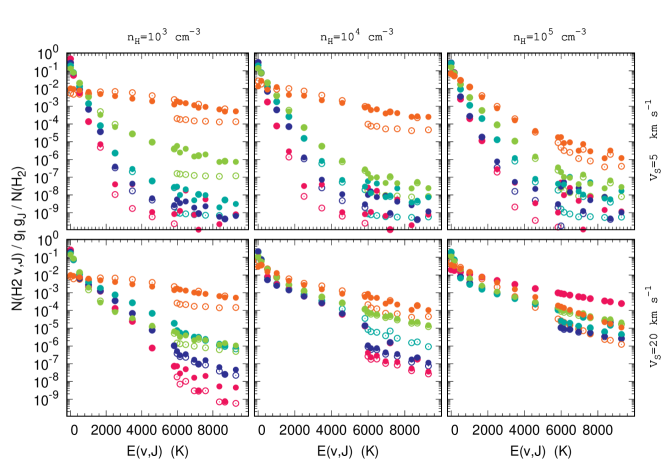
Figure 8: $\rm H_{2}$ excitation diagrams normalized to the column density of $\rm H_{2}$ obtained for shocks propagating at 5 (top panels) and 20 (bottom panels) km s^-1 in media with densities varying between $10^{3}$ (left panels) and $10^{5}$ (right panels) $\,{\rm cm}^{-3}$, a scaling factor of the UV radiation field of $1$ (red), 10 (dark blue), $10^{2}$ (light blue), $10^{3}$ (green), and $10^{4}$ (orange), and a buffer visual extinction $A_{V}^{0}=0.1$. All non-varying parameters are set to their standard values (see Table 1). To estimate the effect of the UV pumping of the rovibrational levels of $\rm H_{2}$, the models have been run with (filled circles) and without (dotted circles) this process. We note that only pure rotational levels exist below 5987 K. Above this limit, both pure rotational and rovibrational levels exist.

The energy budget of molecular shocks is a complex problem that not only depends on the dynamical properties of the shock (velocity and magnetic strength) but also on the medium in which it propagates. Interestingly, all studies performed in dark and dense clouds with $b=0.1$ and $1$ or in environments illuminated by a moderate radiation field converge towards similar results, namely the existence of two regimes depending mostly on the velocity of the shock. At low velocity ($V_{S}\leqslant 5$ km s^-1) most of the kinetic energy dissipates via magnetic compression and through the rotational emission of CO and H₂O (in dark environments, see Pon et al. 2012, 2016; Lehmann & Wardle 2016) or the fine structure lines of C⁺ and O (in media with a moderate radiation field; see Lesaffre et al. 2013). As the velocity increases, the fraction of energy spent in magnetic compression decreases and $\rm H_{2}$ becomes the dominant coolant over a wide range of shock velocities and gas densities (Figs. B1 and B2 of Flower & Pineau des Forêts 2015, and Fig. 8 of Lesaffre et al. 2013).

The results obtained in this work regarding $\rm H_{2}$ emission are in line with those findings, except for large UV radiation fields and in CJ-type shocks where additional processes arise. To illustrate this, in the top panels of Fig. 7 we show the total flux emitted in $\rm H_{2}$ by irradiated shocks normalized to the input flux of kinetic energy. As expected, $\rm H_{2}$ appears as a major coolant over the entire grid of models: although not necessarily dominant, the contribution of $\rm H_{2}$ to the total energy budget is never negligible, varying from about 1% to 90% of the shock initial kinetic energy flux. In concordance with Lesaffre et al. (2013), the contribution of $\rm H_{2}$ is minimal for low velocity shocks where fine structure lines of O and C⁺ take over, and reaches a maximum at higher velocities regardless of the density of the gas. Interestingly, a plateau of $\rm H_{2}$ emission is found over a broad range of radiation field strength, suggesting that as long as the medium is molecular, $\rm H_{2}$ always emits the same fraction of the input mechanical energy. This simple picture breaks, however, when the radiation field is strong enough to dissociate $\rm H_{2}$. At large velocities ($V_{S}\geqslant 10$ km s^-1), the combination of photodissociation and collisional dissociation in CJ-type shocks induces a strong drop in $\rm H_{2}$ abundance. The impact of this drop on $\rm H_{2}$ emission is partly compensated by the increase of the gas temperature which enhances the excitation of $\rm H_{2}$. As a result, the total flux emitted in $\rm H_{2}$ decreases by about a factor of ten only. At lower velocities ($V_{S}\sim 5$ km s^-1), CJ-type shocks are not strong enough to dissociate $\rm H_{2}$ by collisions. In this case, the decrease of $\rm H_{2}$ abundance (due solely to photodissociation) combined with the increase of $\rm H_{2}$ excitation leads to slight variations of the total flux emitted in $\rm H_{2}$.

Two main results therefore emerge from this analysis. Firstly, whatever the physical conditions or the shock type, $\rm H_{2}$ lines systematically carry a significant amount of the shock kinetic energy. Secondly, the radiation field rarely boosts $\rm H_{2}$ emission but may reduce it while increasing its excitation.

The latter behaviour is shown in Fig. 8 which presents the normalized $\rm H_{2}$ excitation diagrams computed in different irradiation conditions. At low radiation fields, the excitation diagrams of $\rm H_{2}$ predicted in C-type shocks generally break in two parts: the low rotational levels which are mainly excited by inelastic collisions, and the remaining rovibrational levels whose populations result from a combination of inelastic collisions, chemical pumping, and UV pumping. As the radiation field increases, the temperature of the gas rises (see Figs. 4 &. 19) and the contribution of inelastic collisions to the excitation of high energy levels increases. This process, combined with the enhancement of the UV pumping, drastically changes the excitation conditions. Indeed, we find that varying the input radiation between $G_{0}=1$ and $G_{0}=10^{4}$ almost leads to a continuum of excitation temperatures, and amplifies the intensities of the rovibrational lines, by several orders of magnitude, for all densities and shock velocities. Interestingly, the contribution of inelastic collisions may become comparable or even larger than that of UV pumping, especially at large density or in high velocity CJ-type shocks (e.g. $V_{S}=20$ km s^-1, ${n_{\rm H}}>10^{4}$ $\,{\rm cm}^{-3}$) where the input mechanical energy strongly overpowers that of the UV photons (see Sect. 5.1).

The impact of shocks on the excitation of $\rm H_{2}$ in outflows has been the subject of many studies (e.g. Flower et al. 2003; Neufeld et al. 2007; Gusdorf et al. 2008b) which show that the excitation diagrams produced by stationary J-type or non-stationary CJ-type shocks are flatter than those obtained in C-type shocks with the same velocities. These studies have concluded that the comparison between observations and predictions can be a powerful tool to derive the properties of jets and the age of the associated astrophysical systems. The results obtained in this work provide a similar tool for irradiated environments. As the radiation field increases and the shock shifts from a C-type to CJ-type structure, the excitation diagram of $\rm H_{2}$ flattens. Strong degeneracies appear, implying that the sole observation of $\rm H_{2}$ excitation, although useful, is not sufficient to circumvent a unique set of physical conditions. The clear identification of irradiated shocks requires complementary data, such as the total emission of $\rm H_{2}$ and the emission and excitation diagrams of other molecules, such as $\rm CH^{+}$.

4.2 CH⁺

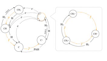
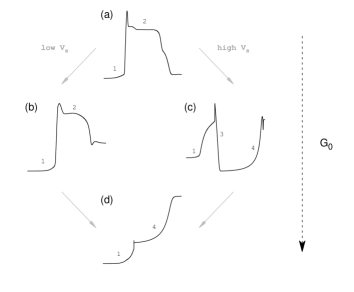
Figure 9: Top: Dominant formation and destruction pathways of the carbon hydrogenation chain in high temperature media ($T\geqslant 250$ K) or in media irradiated by strong UV radiation field. Bottom: Common forms of the density profile of CH⁺ in molecular shocks irradiated by an external radiation field of strength G₀. Although the scales are arbitrary, all the density profiles are shown in log-log space. Labels highlight parts of the trajectory where the evolution of CH⁺ abundance is driven by a specific thermochemical process (see text).

The methylidyne cation $\rm CH^{+}$ is a unique molecule and a golden goose for the study of dissipation of mechanical energy (e.g. Godard et al. 2014; Falgarone et al. 2017). This view stems, first and foremost, from the simplicity of its chemistry summarized in the top panel of Fig. 9. In irradiated environments, the carbon hydrogenation chain can be seen as a series of chemical cycles: a global cycle which controls the hydrogenation of $\rm C^{+}$ and C and the balance between ionized and neutral species, and subcycles which affect how the carbon is distributed over the different hydrides. Seen like this, the global production/destruction of $\rm CH^{+}$, $\rm CH_{2}^{+}$, and $\rm CH_{3}^{+}$ is driven by only three mechanisms: the hydrogenation of $\rm C^{+}$, the destruction of $\rm CH^{+}$ by collision with H, and the dissociative recombinations of $\rm CH_{2}^{+}$ and $\rm CH_{3}^{+}$. The global production rate of $\rm CH^{+}$, $\rm CH_{2}^{+}$, and $\rm CH_{3}^{+}$ is therefore proportional to the abundances of $\rm H_{2}$ and $\rm C^{+}$, and their destruction directly proportional to the abundance of electrons. The way carbon is spread over these three hydrides then depends on the strength of the subcycle highlighted in the top right panel of Fig. 9, hence on the electronic fraction (which favours $\rm CH^{+}$), the molecular fraction (which favours $\rm CH_{3}^{+}$), and the amount of UV photons (which favours $\rm CH^{+}$ through the photodissociation of $\rm CH_{3}^{+}$). As a result, the density profiles of $\rm CH^{+}$ in irradiated shocks can be reduced, over the entire grid of models, to only four different categories (bottom panel of Fig. 9), driven by very few thermochemical processes whose importance mostly depends on the velocity of the shock and strength of the external radiation field.

In molecular shocks, both the ion-neutral velocity drift and the increase of temperature induced by the dissipation of mechanical energy activate the endothermic reaction

$${\rm C^{+}}+{\rm H_{2}}\rightarrow{\rm CH^{+}}+{\rm H}\qquad{\frac{\Delta E}{k_{B}}=4640\,\,{\rm K}}.$$ (34)

This induces a rise in the abundance of $\rm CH^{+}$ (label 1 in Fig. 9) and eventually a fall in that of $\rm C^{+}$. At a low radiation field or low velocity (schemes a and b of Fig. 9), the abundance of $\rm CH^{+}$ reaches a plateau (label 2) $-$ somehow lower than the maximal abundance (due to the destruction of $\rm C^{+}$) $-$ whose size is given by the cooling timescale of the gas. At a large radiation field or large velocity (schemes c and d), the collisional dissociation of $\rm H_{2}$ shuts reaction (34) off. The abundance of $\rm CH^{+}$ rises then drops (label 3) and reaches a plateau whose size is given by the formation timescale of $\rm H_{2}$ (label 4). Because of the subcycle described above and the feedback induced by the photodissociation of $\rm CH_{3}^{+}$, the peak of $\rm CH^{+}$ abundances drastically increases with $G_{0}$. The column density of $\rm CH^{+}$ computed across the shock therefore also increases with $G_{0}$, but only as long as $G_{0}$ and $V_{S}$ are small enough to prevent the collisional dissociation of $\rm H_{2}$, i.e. as long as the shock is either C or C*.

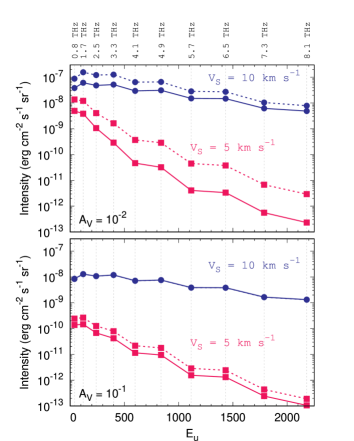
Figure 10: Specific intensities of the first ten rotational lines of $\rm CH^{+}$ (from $J=1\rightarrow 0$ to $J=10\rightarrow 9$) as functions of the upper level energy expressed in Kelvin, emitted by two shocks propagating at 5 (red squares) and 10 (blue circles) km s^-1 in a medium with density of $10^{4}$ $\,{\rm cm}^{-3}$ and illuminated by a radiation field $G_{0}=10^{2}$ at a visual extinction $A_{V}^{0}=0.01$ (top panel) and 0.1 (bottom panel). All other parameters are set to their standard values (see Table 1). The predictions are shown with (dashed) and without (solid) taking into account the UV pumping of the rovibrational levels of $\rm H_{2}$. The corresponding frequency of each rotational line is indicated above the figure.

As shown in Fig. 7, this chemical result directly translates into the efficiency of shocks at producing and exciting $\rm CH^{+}$. As the surrounding UV radiation field increases by a factor of 1000, the total flux emitted in $\rm CH^{+}$ rises by several orders of magnitude $-$ for a given input of mechanical energy $-$ and reaches a maximum at roughly the conditions where CJ-type shocks appear. Because the critical densities of the rotational levels of $\rm CH^{+}$ are large ($\geqslant 10^{7}$ $\,{\rm cm}^{-3}$; Godard & Cernicharo 2013), this effect is magnified in high density media where the high production rate of $\rm CH^{+}$ is combined with high excitation rates. In these conditions, $\rm CH^{+}$ is found to radiate as much as several percent of the shock kinetic energy, a value that is almost comparable to the total flux emitted in $\rm H_{2}$. Altogether, we find that irradiated C or C*-type shocks propagating in dense media (with $G_{0}/{n_{\rm H}}\sim 0.05$ cm³) are the most efficient structures, in terms of energy, for the formation and excitation of $\rm CH^{+}$, hence the structures most likely to be seen in unresolved observations of interstellar environments. Large efficiencies can be obtained at all shock velocities, indicating that the sole observation of the total emission of $\rm CH^{+}$ is not sufficient to identify specific types of shocks.

This degeneracy could be solved, however, by looking at the excitation diagram of $\rm CH^{+}$. Indeed, as shown in Fig. 10, increasing the shock velocity from 5 to 10 km s^-1 $-$ hence the kinetic energy flux by a factor of 8 $-$ drastically enhances the emission of the mid-$J$ lines of $\rm CH^{+}$ whose intensities raise by several orders of magnitude. Observations of the total emission of $\rm CH^{+}$ and of the slope of its excitation diagram could therefore be a powerful tool to infer the type and number of shocks in a given environment, and thus deduce the total mechanical energy pervading the medium. Given the line frequencies indicated in Fig. 10, such measurements could be achieved in galactic environments using the GREAT, FIFI-LS, and HIRMES instruments on board the SOFIA telescope or in extragalactic sources at high redshift using the ALMA interferometer.

4.3 OH, H₂O, CO, and SH⁺

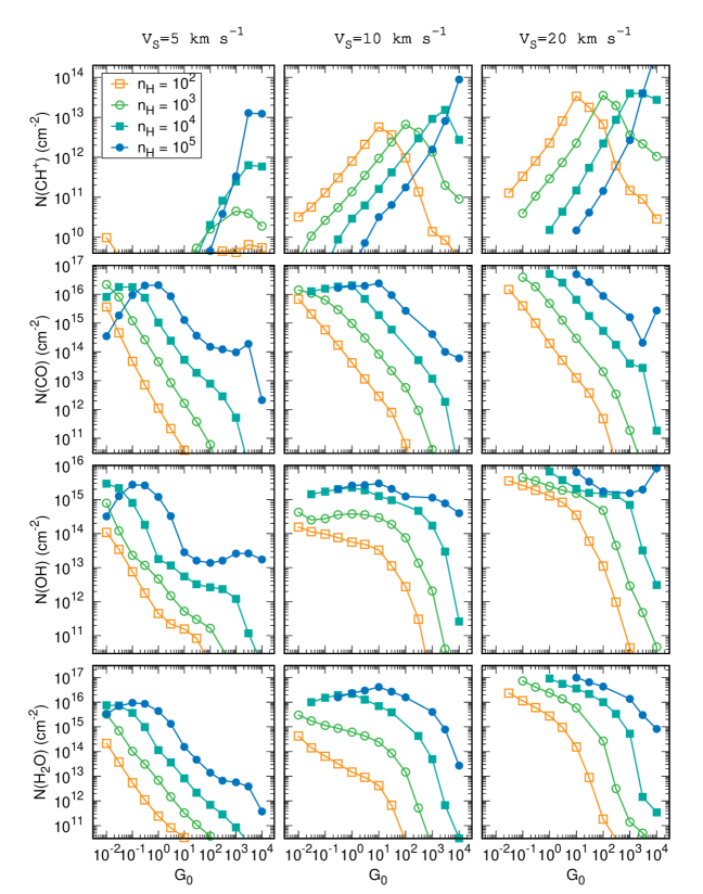
Figure 11: Column densities of $\rm CH^{+}$, CO, OH, and H₂O calculated across shocks propagating at 5 (left panels), 10 (middle panels), and 20 (right panels) km s^-1 in media of density ${n_{\rm H}}=10^{2}$ (empty orange squares), $10^{3}$ (empty green circles), $10^{4}$ (filled green squares), and $10^{5}$ (filled blue circles) $\,{\rm cm}^{-3}$, as function of the impinging radiation field $G_{0}$, and for a buffer visual extinction $A_{V}^{0}=0.1$. All other parameters are set to their standard values (see Table 1).

Table 2: Total hydrogen column density $N_{\rm H}$ and column densities of several species computed across irradiated shocks propagating in a medium of density ${n_{\rm H}}=10^{4}$ $\,{\rm cm}^{-3}$ at a visual extinction $A_{V}^{0}=0.1$. All other parameters are set to their standard values (Table 1). Numbers in parenthesis are powers of ten.

	$N_{\rm H}$	$N({\rm H}_{2})$	$N({\rm C^{+}})$	$N({\rm CH^{+}})$	$N({\rm SH^{+}})$	$N({\rm O})$	$N({\rm O}_{2})$	$N({\rm OH})$	$N({\rm H}_{2}{\rm O})$	$N({\rm CO})$
	cm-2	cm-2	cm-2	cm-2	cm-2	cm-2	cm-2	cm-2	cm-2	cm-2
$V_{S}$ = 5 km s-1
$G_{0}=1$	5.6 (20)	2.8 (20)	4.0 (14)	2.5 (08)	1.3 (10)	1.6 (17)	2.8 (13)	1.8 (13)	1.1 (14)	1.0 (15)
$G_{0}=10$	1.3 (20)	6.5 (19)	1.1 (15)	5.5 (08)	3.9 (08)	3.9 (16)	1.1 (12)	5.5 (12)	8.2 (12)	5.3 (13)
$G_{0}=100$	5.8 (19)	2.8 (19)	3.7 (15)	2.0 (10)	3.7 (07)	1.8 (16)	3.5 (10)	2.6 (12)	6.9 (11)	7.9 (12)
$G_{0}=1000$	4.3 (19)	1.2 (19)	5.7 (15)	2.5 (11)	1.7 (07)	1.3 (16)	1.4 (09)	1.2 (12)	8.4 (10)	5.2 (11)
$V_{S}$ = 10 km s-1
$G_{0}=1$	6.6 (20)	3.3 (20)	1.4 (14)	2.9 (10)	5.4 (11)	1.4 (17)	1.6 (15)	2.2 (15)	2.2 (16)	2.0 (16)
$G_{0}=10$	2.6 (20)	1.3 (20)	6.1 (14)	1.6 (11)	3.0 (12)	6.9 (16)	6.1 (12)	1.3 (15)	6.9 (15)	1.9 (15)
$G_{0}=100$	3.1 (20)	1.3 (20)	4.8 (15)	1.1 (12)	1.1 (13)	9.5 (16)	1.1 (14)	7.8 (14)	1.9 (15)	3.4 (14)
$G_{0}=1000$	4.2 (19)	1.2 (19)	4.0 (15)	9.1 (12)	1.6 (12)	1.3 (16)	1.8 (11)	1.7 (14)	4.9 (13)	1.2 (13)
$V_{S}$ = 20 km s-1
$G_{0}=1$	8.4 (20)	4.2 (20)	2.1 (13)	1.5 (10)	8.6 (11)	8.2 (16)	5.8 (15)	6.6 (15)	9.0 (16)	5.1 (16)
$G_{0}=10$	7.7 (20)	3.8 (20)	7.1 (14)	1.5 (11)	3.6 (12)	1.8 (17)	3.4 (14)	2.1 (15)	3.6 (16)	6.4 (15)
$G_{0}=100$	2.9 (20)	1.3 (20)	3.1 (15)	2.2 (12)	1.9 (13)	7.5 (16)	1.2 (13)	1.5 (15)	9.9 (15)	5.3 (14)
$G_{0}=1000$	6.5 (19)	1.8 (19)	4.0 (15)	4.0 (13)	3.4 (13)	1.8 (16)	7.6 (11)	7.0 (14)	5.3 (14)	3.9 (13)

The specificity of $\rm CH^{+}$ chemistry makes irradiated shocks efficient factories of $\rm CH^{+}$. The same does not hold for all molecules, and in particular those efficiently destroyed by UV photons. To illustrate this, we compare in Fig. 11 the column densities of $\rm CH^{+}$ computed across molecular shocks to those of CO, OH, and H₂O. As already shown by Falgarone et al. (2010), the increase of the column density of $\rm CH^{+}$ with increasing values of $G_{0}$ almost systematically comes with a decrease of the column densities of CO, OH, and H₂O. The associated drop can cover one to several orders of magnitude depending on the medium density and velocity of the shock. We find that the column density of $\rm CH^{+}$ linearly increases with $G_{0}$ up to a maximal value, while the decrease of the column density of CO, OH, and H₂O is steeper, especially at high $G_{0}$ and large $V_{S}$.

The predicted values obtained for ${n_{\rm H}}=10^{4}$ $\,{\rm cm}^{-3}$ and $1\leqslant G_{0}\leqslant 10^{3}$ are reported in Table 2, along with the predictions on the total hydrogen column density $N_{\rm H}$ and the column densities of $\rm H_{2}$, $\rm C^{+}$, $\rm SH^{+}$, O, and O₂. The column density ratios $N({\rm H}_{2}{\rm O})/N({\rm OH})$ and $N({\rm CO})/N({\rm OH})$ appear to decrease strongly with $G_{0}$, a result in line with Melnick & Kaufman (2015) who find similar behaviour in dense environments illuminated by moderate radiation fields (${n_{\rm H}}=10^{5}$ $\,{\rm cm}^{-3}$, $G_{0}\leqslant 10$). Table 2 reveals that other chemical species follow $\rm CH^{+}$ and are strongly enhanced in irradiated shocks. This is the case, for instance, of the mercapto cation $\rm SH^{+}$. For a shock velocity larger than 10 km s^-1, the predicted column density of $\rm SH^{+}$ is found to increase with $G_{0}$, although with a power-law slope somehow shallower ($N({\rm SH^{+}})\propto\sqrt{G_{0}}$) than that found for $\rm CH^{+}$. All these results indicate that irradiated shocks carry many specific chemical signatures that could be identified using the current observing facilities.

5 Discussion

5.1 Kinetic and radiative energies budget

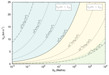
Figure 12: Isocontours of the ratio of the initial kinetic energy flux contained in an interstellar shock to the radiative energy flux contained in ultraviolet photons, $\mathscr{F}_{\rm K}(0)/\mathscr{F}_{\rm UV}$, where $\mathscr{F}_{\rm UV}=7.7\times 10^{-4}G_{0}$ erg cm^-2 s^-1, as a function of $G_{0}$, the shock speed $V_{S}$, and the pre-shock density ${n_{\rm H}}$ (indicated on the isocontours). The dashed region corresponds to the parameter domain, for ${n_{\rm H}}=10^{4}$ $\,{\rm cm}^{-3}$, where the amount of UV radiative energy reprocessed into heat within a shock is larger (on average) than the amount of mechanical energy reprocessed into heat (Eq. 36).

Establishing the energy budget of irradiated molecular shocks is complex. In the previous sections, the results on the molecular lines emission were systematically presented with respect to the initial kinetic energy flux of the shock (see Fig. 7). The underlying interpretation was that shock radiative emission is an outcome of the reprocessing of mechanical energy only. This view could be misleading as the matter contained in irradiated shocks also reprocesses part of the input UV radiative energy.

To discuss this point, we compare in Fig. 12 the initial kinetic energy flux of shocks with the radiative energy flux contained in the ambient UV field depending on the model parameters. The grid of physical conditions explored in this work clearly covers a broad range of scenarios in which the input kinetic energy flux is either equal to, greater than, or less than the flux contained in the UV field. In what proportion these energy sources are converted into molecular lines over the duration of a shock depends on the reprocessing lengths and efficiency of energy conversion.

To simplify, we perform estimations of these quantities considering only reprocessing into thermal energy, i.e. assuming that atomic and molecular lines primarily result from the gas heating. This approach is valid as long as the radiative pumping is not the dominant excitation process of the species considered.

By definition (see Eq. 29), the input mechanical energy is entirely reprocessed over the size of the shock, shown in Fig. 6. For shock velocity larger than 5 km s^-1, and standard magnetization ($b=1$), the fraction of energy spent in magnetic compression is found to be smaller than a few tens of percent (Lesaffre et al. 2013). The mechanical energy is therefore mostly converted into atomic and molecular lines with an efficiency of several tens of percent, a value that increases with the speed of the shock. In contrast, the radiative energy contained in UV photons is reprocessed by grains over about one magnitude of extinction which corresponds to distances,

$$l_{\rm UV}\sim 12\times 10^{3}\,\,{\rm au}\,\,\left(\frac{{n_{\rm H}}}{10^{4}{\,{\rm cm}^{-3}}}\right)^{-1},$$ (35)

10 to 100 times larger than the shock sizes. In this case, the amount of radiative energy converted into thermal energy of the gas is given by the efficiency of the photoelectric effect which ranges between 2 and 7% (e.g. Ingalls et al. 2002). Putting together all these characteristics, we find that the amount of radiative energy reprocessed into heat dominates, on average, the amount of mechanical energy reprocessed into heat for

$$\frac{G_{0}}{{n_{\rm H}}}\left(\frac{V_{S}}{5\,{\,{\rm km}\,{\rm s}^{-1}}}\right)^{-3}\geqslant 0.1\,\,{\rm cm}^{3},$$ (36)

i.e. over a small fraction of our grid of models, at low density, low shock velocity, and large radiation field intensity (see Fig. 12).

This result is particularly well illustrated in Fig 19. The input kinetic energy fluxes of the models explored in this work are found to be always sufficient to modify the thermal state of the gas. The relative increase of the gas temperature can be, however, quite small in low velocity shocks propagating in strongly irradiated environments (e.g. $V_{S}=5$ km s^-1 and $G_{0}=10^{4}$) where the maximal temperature reached in the shock is almost identical to that found in the post-shock gas. This happens because the heating rate induced by UV photons is locally comparable to that induced by the dissipation of mechanical energy. In this case, the sole impact of the shock is to slightly compress the gas, increasing its thermal pressure and modifying its coupling with the external UV field. Except for kinematic signatures, shocks in these environments are probably undetectable because they do not impact significantly the thermochemical state of the gas.

5.2 J-type shocks and self-generated UV radiation field

The model presented in this work contains all the necessary ingredients to compute the local emission and absorption of photons by gas and dust particles. It is, however, important to stress that neither the feedback of the photons produced by the shock itself on the surrounding material nor the radiative transfer of these photons within the shock are currently treated. This caveat strongly limits the upper range of J-type shocks velocities that can be studied with the Paris-Durham shock code.

The adiabatic jump conditions (Eq. 28) imply that the temperature reached in J-type shocks are often large enough to either ionize chemical species or excite their electronic levels (Shull & McKee 1979). These mechanisms, followed by radiative recombinations and radiative decay, induce the production of high energy photons that heat, dissociate, or ionize the gas within the shock, but also in the pre-shock and post-shock media, leading to the formation of a radiative precursor (Neufeld & Dalgarno 1989; Hollenbach & McKee 1989; Draine & McKee 1993).

Without magnetic field, J-type shocks with velocities larger than 25 km s^-1 emit Ly $\alpha$ and Ly $\beta$ photons (Shull & McKee 1979). Their energies are strong enough to enhance the photoelectric effect, hence the temperature of the pre-shock gas, and the dissociation and ionization of many species. For shocks propagating at 30 km s^-1 in a medium of density ${n_{\rm H}}=2\times 10^{5}$ $\,{\rm cm}^{-3}$, Flower & Pineau des Forêts (2010) estimated a UV flux of $10^{11}$ photons cm^-2 s^-1, corresponding to an equivalent $G_{0}=10^{3}$. Such an effect cannot be neglected.

Finding a self-consistent solution requires building an iterative procedure to compute the photon flux emitted by the shock and also to construct a radiative code capable of solving the transfer and the scattering of Ly $\alpha$ and Ly $\beta$ photons and other optically thick lines. We deliberately chose to limit our analysis to low velocity C-, C*, and CJ-type shocks ($V_{S}\leqslant 25$ km s^-1) where the production of high energy photons is negligible. All these developments are however in progress and will be the subject of a forthcoming paper on self-irradiated shocks.

6 Conclusions

We have built a model designed to compute the dynamics and thermochemistry of molecular shocks in environments irradiated by an external UV radiation field. The framework is that of a plane-parallel shock at steady-state propagating at a given position of a plane-parallel PDR. The steady-state solutions of magnetohydrodynamics equations are computed through a new and convoluted algorithm capable of following the evolution of the gas near and through sonic points and along subsonic trajectories of molecular shocks. The resulting code allows the simultaneous and self-consistent treatment of gas dynamics and chemistry and of the radiative transfer in a wide variety of physical conditions including diffuse clouds and dense and hot PDRs. It therefore provides a unique tool to study the combined effect of radiative and mechanical energy on the thermochemistry of interstellar matter.

Ultraviolet photons exert an impact on molecular shocks that goes far beyond ionization and dissociation: they modify the structure of the shock itself. Because of the combined effects of dynamics and photoprocesses, irradiated C-type shocks shrink with the strength of the radiation field. If the cooling is not strong enough, the gas may become subsonic along the trajectory. This induces the formation of unexplored categories of stationary shocks called C*-type or CJ-type, depending on whether the sonic point is crossed continuously or not. These types of shocks are dominant in weakly magnetized, diffuse, or irradiated environments. We find, for instance, that only low velocity C-type shocks ($V_{S}\leqslant 5$ km s^-1) can exist in typical PDRs (${n_{\rm H}}\sim 10^{4}$ $\,{\rm cm}^{-3}$, $G_{0}\sim 100$) or in very diffuse clouds (${n_{\rm H}}\sim 30$ $\,{\rm cm}^{-3}$, $G_{0}\sim 1$) at low extinction and for standard magnetic field strengths ($b=1$) ; higher velocity shocks are either C* or CJ (for $5\leqslant V_{S}\leqslant 25$ km s^-1), or J (for $V_{S}\geqslant 25$ km s^-1).

The increase of the photodissociation of $\rm H_{2}$ and the diminution of the shock size with increasing UV field, lead to larger temperature which eventually triggers the collisional dissociation of $\rm H_{2}$ even at low velocity. All these processes strongly influence the energy budget of shocks but also the chemistry and excitation of atomic and molecular lines. Several molecules, such as CO, OH, and H₂O, are found to be destroyed too quickly by UV photons to be efficiently produced in irradiated shocks, while the formations of others, such as $\rm CH^{+}$ and $\rm SH^{+}$, are boosted by the entwined actions of kinetic and radiative energies.

The best diagnostics of irradiated shocks are probably the rotational lines of $\rm CH^{+}$. The combination of high production and excitation rates drastically change the efficiency of $\rm CH^{+}$ emission which can carry, at large density, as much as several percent of the shock kinetic energy. The distribution of $\rm CH^{+}$ emission over its different rotational lines is found to be highly sensitive to the shock velocity, hence providing a unique set of tracers of shock kinetic energy.

One unexpected result is the weak sensitivity of the total $\rm H_{2}$ emission to the input UV radiation field, combined with the strong sensitivity of its excitation diagram. This finding extends the results of previous studies on the excitation of $\rm H_{2}$ and offers a reliable criterion to infer the irradiation conditions of known interstellar shocks that can be tested with the impending launch of the JWST.

The analysis of the shock energy balance reveals the strong interplay of radiative and mechanical energies. In most cases, molecular line emissions result from the conversion of the shock mechanical energy while this conversion is affected by the impinging UV field. This ceases to be true, however, at low velocity, low density, or large radiation fields where the input UV radiative energy reprocessed by the shock itself becomes dominant.

The work presented in this paper sheds new light on the interpretation of line emission and provides new templates for the analysis of observations. It calls, however, for several developments. Deliberately limited to a handful of species, it would be interesting to extend our analysis to a more systematic study of the chemistry and address, for instance, the formation and excitation of other known tracers of shocks and turbulent dissipation, such as SiO, $\rm SH^{+}$, and $\rm HCO^{+}$. Similarly, it will soon be essential to broaden the exploration of the physical conditions to unveil the signatures of high velocity irradiated J-type shocks and those of shocks propagating in highly and weakly magnetized media. One of the most promising applications is the disentanglement of the contribution of stellar radiation and mechanical feedback in the emission bulk of galaxies in order to establish their energy budget and understand the nature of their chemical complexity.

Appendix A Grain size distribution

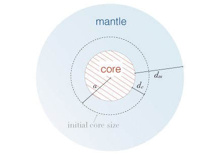
Figure 13: Schematic view of erosion and adsorption on grains.

All processes involving grains are treated using a prescription similar to that proposed by Le Bourlot et al. (1995). As drawn on Figure 13, we assume spherical grains composed of mineral cores and surrounded by ice mantles. Shattering and coagulations processes are neglected. Erosion processes are supposed to reduce evenly the initial size of the cores by a thickness $d_{e}$, while adsorption and desorption mechanisms are supposed to build evenly mantles on cores over a thickness $d_{m}$.

We assume that the grain cores follow a power-law size distribution from a minimal size $a_{\rm m}$ to a maximal size $a_{\rm M}$. At the ionization front (see Fig. 1), the initial number of cores per unit volume of gas with radii between $a$ and $a+da$, $dn_{g}^{0}(a)$, is

$$dn_{g}^{0}(a)=Aa^{-\alpha}da.$$ (37)

With the initial condition $d_{e}=d_{m}=0$, the integration of the grain mass over the size distribution leads to the normalization coefficient

$$A=\frac{3}{4\pi\rho_{c}f_{4}}\sum_{i}m({\rm X}_{i}^{**})n^{0}({\rm X}_{i}^{**}),$$ (38)

where

$$f_{n}=\frac{a_{\rm M}^{n-\alpha}-a_{\rm m}^{n-\alpha}}{n-\alpha}.$$ (39)

$m({\rm X}_{i}^{**})$ and $n^{0}({\rm X}_{i}^{**})$ are the masses and initial densities of the chemical species ${\rm X}_{i}^{**}$ which compose the core, and ${\rho_{c}}$ is the core mass density, assumed to be homogeneous and identical for all grains. The initial number of grains per unit volume of gas therefore writes

$$n_{g}^{0}=Af_{1}.$$ (40)

Starting from these initial conditions, the evolution of dust grains is computed in the buffer and in the shock taking into account several processes: i.e. adsorption, desorption, and erosion, which modify the thicknesses $d_{e}$ and $d_{m}$, and the compression induced by the shock. Defining $\mathscr{C}_{g}$ as the compression factor of the grain fluid, the number of grains $n_{g}$ per unit volume of gas writes

$$n_{g}=Af_{1}\mathscr{C}_{g}.$$ (41)

If we assume that erosion, adsorption, and desorption mechanisms only depend on geometrical cross sections, the integration of the corresponding rates over the size distribution reduces to the calculation of the rate for a single grain of radius $\langle r_{c}^{2}\rangle^{1/2}$ (for grain core processes) and $\langle r_{m}^{2}\rangle^{1/2}$ (for grain mantle processes), where

$$\langle r_{c}^{2}\rangle=\frac{\int_{a_{\rm m}}^{a_{\rm M}}(a-d_{e})^{2}a^{-\alpha}da}{\int_{a_{\rm m}}^{a_{\rm M}}a^{-\alpha}da}$$ (42)

is the mean square radius of eroded grain cores and

$$\langle r_{m}^{2}\rangle=\frac{\int_{a_{\rm m}}^{a_{\rm M}}(a-d_{e}+d_{m})^{2}a^{-\alpha}da}{\int_{a_{\rm m}}^{a_{\rm M}}a^{-\alpha}da}$$ (43)

is the mean square radius of grains including mantles. The integration of those equations yields analytical expressions relating $\langle r_{c}^{2}\rangle$ and $\langle r_{m}^{2}\rangle$ to $d_{e}$ and $d_{m}$, i.e.

$$\langle r_{c}^{2}\rangle=\frac{1}{f_{1}}\left[f_{3}-2f_{2}de+f_{1}d_{e}^{2}\right]$$ (44)

and

$$\langle r_{m}^{2}\rangle=\frac{1}{f_{1}}\left[f_{3}+2f_{2}(d_{m}-de)-2f_{1}d_{e}d_{m}+f_{1}(d_{e}^{2}+d_{m}^{2})\right].$$ (45)

According to the geometrical and chemical models, the volume of grain cores removed by the erosion mechanisms (per unit volume of gas) is

$$\mathcal{V}_{e}=\mathscr{C}_{g}\int_{a_{\rm m}}^{a_{\rm M}}A\frac{4\pi}{3}\left[a^{3}-(a-d_{e})^{3}\right]a^{-\alpha}da$$ (46)

and

$$\mathcal{V}_{e}=\frac{1}{\rho_{c}}\sum_{i}m({\rm X}_{i}^{**})\left(\mathscr{C}_{g}n^{0}({\rm X}_{i}^{**})-n({\rm X}_{i}^{**})\right),$$ (47)

which leads to a cubic equation for $d_{e}$

$$3f_{3}d_{e}-3f_{2}d_{e}^{2}+f_{1}d_{e}^{3}=f_{4}\left(1-\frac{\sum_{i}m({\rm X}_{i}^{**})n({\rm X}_{i}^{**})}{\sum_{i}m({\rm X}_{i}^{**})n^{0}({\rm X}_{i}^{**})\mathscr{C}_{g}}\right).$$ (48)

Similarly, the volume of grain mantles writes

$$\mathcal{V}_{m}=\mathscr{C}_{g}\int_{a_{\rm m}}^{a_{\rm M}}A\frac{4\pi}{3}\left[(a-d_{e}+d_{m})^{3}-(a-d_{e})^{3}\right]a^{-\alpha}da$$ (49)

and

$$\mathcal{V}_{m}=\frac{1}{\rho_{m}}\sum_{i}m({\rm X}_{i}^{*})n({\rm X}_{i}^{*}),$$ (50)

where $\rho_{m}$ is the mantle mass density and $m({\rm X}_{i}^{*})$ and $n({\rm X}_{i}^{*})$ are the masses and densities (per unit volume of gas) of the chemical species ${\rm X}_{i}^{*}$ which compose the mantle. The development of those equations finally leads to a cubic expression for $d_{m}$

$$3f_{3}d_{m}-6f_{2}d_{e}d_{m}+3f_{1}d_{e}^{2}d_{m}+3f_{2}d_{m}^{2}-3f_{1}d_{e}d_{m}^{2}+f_{1}d_{m}^{3}=f_{4}\frac{\rho_{c}}{\rho_{m}}\frac{\sum_{i}m({\rm X}_{i}^{*})n({\rm X}_{i}^{*})}{\sum_{i}m({\rm X}_{i}^{**})n^{0}({\rm X}_{i}^{**})\mathscr{C}_{g}}.$$ (51)

Table 3: Parameters of the grain size distribution model and initial abundances $x({\rm X}_{i}^{**})$ of grain core compounds. Numbers in parenthesis are powers of ten.

Parameter	value		unit	ref
$\alpha$	-3.	5		a
$a_{\rm m}$	1.	0 (-6)	cm	a
$a_{\rm M}$	3.	0 (-5)	cm	a
$\rho_{c}$	2.	0	g cm-3	b
$\rho_{m}$	1.	0	g cm-3	b
$x^{0}({\rm O}^{**})$	1.	40 (-4)		c
$x^{0}({\rm Si}^{**})$	3.	37 (-5)		c
$x^{0}({\rm Mg}^{**})$	3.	70 (-5)		c
$x^{0}({\rm Fe}^{**})$	3.	23 (-5)		c
$x^{0}({\rm C}^{**})$	1.	63 (-4)		c

• $a$ $-$ Mathis et al. (1977), $b$ $-$ Hily-Blant et al. (2018), $c$ $-$ Flower & Pineau des Forêts (2003)

In the Paris-Durham shock code, equations 48 and 51 are solved at each time step using a Newton-Raphson scheme. The values of $d_{e}$ and $d_{m}$ are then injected in equations 44 and 45 to compute the mean square radii of the cores and mantles and the subsequent erosion, adsorption, and desorption rates, which control the evolution of the ${\rm X}_{i}^{**}$ and ${\rm X}_{i}^{*}$ abundances over the next time step. All the parameters used in this work are given in Table 3. The initial abundances of the grain core compounds correspond to an initial dust-to-gas mass ratio of 0.56 %.

Erosion of grain mantles, adsorption, and photodesorption processes for grains of size $a_{g}$ and relative abundance $x_{g}$ occur over characteristic timescales, roughly given by (Barlow 1978; Flower et al. 2005; Hollenbach et al. 2009)

$$\mathscr{T}_{\rm ero}\sim 5\times 10^{-1}\left(\frac{10^{4}\,{\,{\rm cm}^{-3}}}{{n_{\rm H}}}\right)\left(\frac{10^{-6}\,{\rm cm}}{a_{g}}\right)^{2}\\ \left(\frac{10^{6}\,{\rm cm\,\,s^{-1}}}{\Delta v}\right){\rm exp}\left[3\left(\frac{10^{6}\,{\rm cm\,\,s^{-1}}}{\Delta v}\right)^{2}\right]\,\,{\rm yr},$$ (52)

$$\mathscr{T}_{\rm ads}\sim 3\times 10^{6}\left(\frac{10^{4}\,{\,{\rm cm}^{-3}}}{{n_{\rm H}}}\right)\left(\frac{10^{-11}}{x_{g}}\right)\left(\frac{10^{-6}\,{\rm cm}}{a_{g}}\right)^{2}\,\,{\rm yr},\\$$ (53)

and

$$\mathscr{T}_{\rm phd}\sim 2\times 10^{4}\left(G_{0}+4\times 10^{-5}\frac{\zeta_{{\rm H_{2}}}}{3\times 10^{-17}s^{-1}}\right)^{-1}\left(\frac{10^{-6}\,{\rm cm}}{a_{g}}\right)^{2}\,\,{\rm yr},$$ (54)

where $\Delta v$ is the velocity difference between the ions and neutrals. Those values compared with the dynamical timescales given in Fig. 6 show that adsorption never occurs over the duration of a shock, while photodesorption and the erosion of grain mantles may occur within the shock depending on the density of the gas, strength of the radiation field, and ion-neutral velocity drift. It follows that the adsorption processes are important only for the computation of the equilibrium composition of the pre-shock and the post-shock gas, that the erosion processes only arise within the shock where the ions and the neutrals decouple, and that photodesorption may be important everywhere depending on the irradiation conditions.

Appendix B Comparison with PDR models

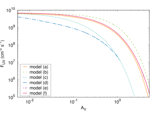
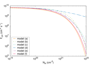
Figure 14: Ultraviolet photon flux (integrated from 911 to 2400 Å) as a function of the total hydrogen column density (bottom panel) and the visual extinction (top panel) calculated with the Meudon PDR code (a), by Tielens & Hollenbach (1985) (b), and with the Paris-Durham shock model set in advection mode (c-f) for an isochoric gas of density ${n_{\rm H}}=10^{4}$ $\,{\rm cm}^{-3}$ with an incident radiation field $G_{0}=10^{2}$. The predictions of the Paris-Durham model are shown for pure graphite grains with a size distribution defined by Table 3 (standard model, labelled c), for silicate grains with the same size distribution (d), graphite grains with a minimal radius set to $3\times 10^{-6}$ cm (e), and graphite grains with a minimal radius set to $3\times 10^{-6}$ cm where the grain absorption coefficients are scaled to impose a $N_{\rm H}/A_{V}$ ratio of $1.87\times 10^{21}$ cm^-2 (f).

To validate the treatment of the radiative transfer and of the multiple interactions of far-UV photons with interstellar matter, we perform comparisons of state-of-the-art PDR models with the predictions of the Paris-Durham shock code set in advection mode. In this mode, the code follows the isochoric or isobaric thermo-chemical evolution of a single fluid moving away from the ionization front with a constant velocity $v_{\rm adv}$. For simplicity, we consider a prototypical isochoric PDR of density ${n_{\rm H}}=10^{4}$ $\,{\rm cm}^{-3}$, illuminated on one side by an isotropic radiation field with a scaling factor $G_{0}=100$, and moving at a speed $v_{\rm adv}=0.01$ km s^-1. Unless indicated otherwise, all adsorption and desorption mechanisms are switched off.

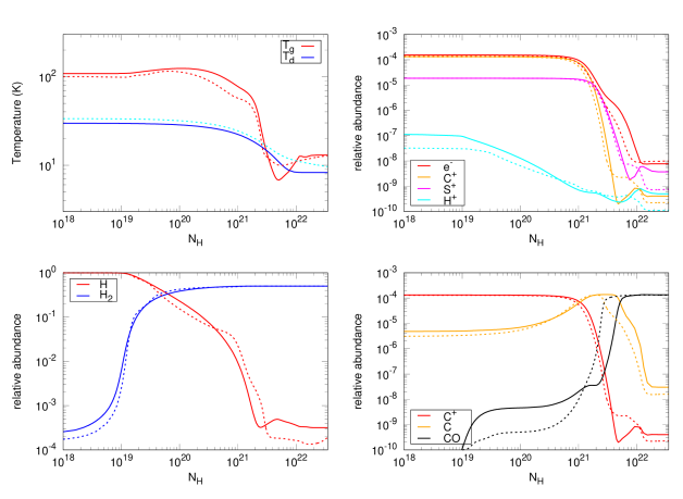
Figure 15: Gas and dust (radius = 0.05 $\mu$m) temperatures (top left panel) and abundances of the main ions, atomic, and molecular compounds (other panels) as functions of the total hydrogen column density computed with the Meudon PDR code (dashed lines) and the Paris-Durham code (continuous lines) for an isochoric PDR of density ${n_{\rm H}}=10^{4}$ $\,{\rm cm}^{-3}$ with an incident radiation field $G_{0}=10^{2}$.

Fig. 14 shows model predictions of the photon flux (integrated between 911 and 2400 Å) as a function of the visual extinction and total hydrogen column density for different models of grains. By default, most of the existing PDR codes tune the grain absorption and scattering coefficients at all wavelengths in order to match the standard galactic extinction curve observed by Fitzpatrick & Massa (1986) and to reproduce a fixed $N_{\rm H}/{A_{V}}$ ratio of $1.87\times 10^{21}$ cm^-2. This is not the case in the shock model where the extinction curve and colour indices are derived from grain properties alone and may differ from one model to the next. Hence, before comparing the predictions we need to choose which of $A_{V}$ or $N_{\rm H}$ is the best natural variable to display PDR profiles. Analysis of the absorption coefficients shows that the ratios of the visible extinction to the extinctions at other wavelengths vary considerably depending on the grain size and composition. As a result, $A_{V}$ is not only weakly representative of the absorption of photons over the entire UV range when the grain model is changed, but is also a poor tracer of the amount of dust in the cloud. In contrast, since the abundance of grains is considered as constant, $N_{\rm H}$ is a natural proxy of the dust column density regardless of the grain size and composition. All the comparisons below will thus be discussed as functions of $N_{\rm H}$.

The comparison of the shock results with classical PDR models in the bottom panel of Fig. 14 shows that almost all the prescriptions of grains adopted in this work, with the exception of pure silicate grains, give satisfactory predictions of the absorption of UV flux as a function of the depth into the cloud. This discrepancy for the pure silicate grain model is due to the absorption properties of dust at large wavelengths. While graphite and silicate have similar absorption coefficients around 1000 Å, that of silicate is up to 100 times smaller than that of graphite at 2000 Å for a grain with radius between 0.01 and 0.1 $\mu$m. The radiation field is thus absorbed over distances considerably larger when silicate grains are used. The best agreement with the Meudon PDR code is obtained for pure graphite grains with a minimal radius set to $3\times 10^{-6}$ cm and where the grain absorption coefficients are scaled homogeneously to impose a $N_{\rm H}/A_{V}$ ratio of $1.87\times 10^{21}$ cm^-2 (model f in Fig. 14).

Keeping this last configuration, we compare the predictions of the Paris-Durham shock model with those of the Meudon PDR code regarding the main physical properties of PDRs, i.e. the temperatures of gas and dust, ionization fraction, H/$\rm H_{2}$ and $\rm C^{+}$/C/CO transitions, and excitation of the rovibrational levels of $\rm H_{2}$. As a whole, Fig. 15 shows a satisfactory agreement between the results of the two models. In particular, the temperature profiles, H/$\rm H_{2}$ transition, and ionization fraction are found to follow the same trends with values almost identical at the border and in the interior of the cloud. All the discrepancies observed, i.e. the difference of about a factor of five in the calculation of the $\rm S^{+}$ abundance in the environment well shielded from the radiation field and the C/CO transition that arises at distances three times larger than in the Meudon PDR code, are due to the different chemical networks and prescriptions of PAHs (e.g. size distribution, calculation of ionization, and recombination processes) used in each model. The populations of the first 200 rovibrational levels of $\rm H_{2}$ computed at the border of the cloud and shown in Fig. 16 are found to be analogous in both models; there is a maximum discrepancy of about a factor of three for the most energetic levels. In summary, these results not only validate the treatments of the radiative processes now performed in the Paris-Durham shock code but also justify the approximation of using a single size grain in the computation of the UV radiative transfer.

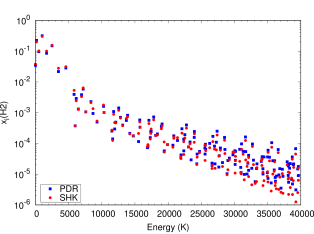
Figure 16: $\rm H_{2}$ level populations as functions of their energies computed with the Meudon PDR code (blue squares) and the Paris-Durham model (red circles) at $N_{\rm H}=1.87\times 10^{15}$ cm^-2, in an isochoric PDR of density ${n_{\rm H}}=10^{4}$ $\,{\rm cm}^{-3}$ with an incident radiation field $G_{0}=10^{2}$.

To check the treatments of the adsorption and desorption processes, we finally compare the solid-phase and gas-phase abundances of a few species (namely CO, CH₄ and H₂O) predicted by the code (when adsorption and desorption are switched on) with those obtained by Hollenbach et al. (2009) (Figs. 3 & 4). In both models, mantles become the main carrier of all heavy elements at similar distances ($\sim 6\times 10^{17}$ cm). Comparable results are also found for gas-phase abundances. Because of the lack of efficient desorption processes in the interior of the cloud ($>2\times 10^{18}$ cm), the two models converge towards a chemical equilibrium with gas-phase abundances below $10^{-7}$ for both carbon and oxygen bearing species. The fact that both models give virtually identical results is surprising in the light of the treatment of photodesorption by secondary UV photons. Indeed, according to Hollenbach et al. (2009), the secondary photon flux associated with a primary cosmic-ray ionization rate of $10^{-17}$ s^-1 in a medium with a density of $10^{4}$ $\,{\rm cm}^{-3}$ is equivalent to $G_{0}\sim 10^{-3}$. In comparison, the treatment we propose in Sect. 2.5 leads to an equivalent radiation field of $G_{0}\sim 10^{-5}$ for the same conditions, close to the value derived by Shen et al. (2004) and that used in Heays et al. (2017). The agreement between the gas-phase abundances computed in both models indicates that this apparent discrepancy is likely to be a typo in Hollenbach’s paper not implemented in their chemical code, which probably uses the correct value, i.e. a secondary photon flux of $2\times 10^{3}$ photons cm^-2 s^-1 for $\zeta_{{\rm H_{2}}}=10^{-17}$ s^-1 and ${n_{\rm H}}=10^{4}$ $\,{\rm cm}^{-3}$.

Appendix C Computation of stationary solutions

The governing equations of partially ionized, plane-parallel, and magnetized molecular shocks have been derived in several papers (e.g. Draine 1980; Flower et al. 1985). Under the assumption of stationarity, they organize into a set of coupled, first-order, ordinary differential equations that fully describe the exchanges of mass, momentum, and energy that occur between the different chemical flows. Together with the initial conditions, the system thus forms an initial value problem which, in principle, may be integrated using a classical forward integration technique (e.g. DVODE, Hindmarsh 1983). As proven with the Paris-Durham shock code (e.g. Flower & Pineau des Forêts 2003, 2015), such a method is highly robust and efficient in computing the steady states of J-type shocks (single fluid) or that of C-type shocks, i.e. shocks where the neutrals and ions are decoupled and where the flow stays supersonic over its entire trajectory. In the case of C-type shocks, this method fails, however, if the cooling is not efficient enough so that the neutral flow becomes subsonic at some point along the trajectory. Indeed, these conditions trigger the emergence of another category of stationary structures, called CJ-type and C*-type shocks (Chernoff 1987; Roberge & Draine 1990). Because these structures require crossing critical points, forward integration techniques become unstable and highly sensitive to numerical errors.

The method we apply to treat CJ-type and C*-type shocks is based on the work of Roberge & Draine (1990) who thoroughly described the physics of shocks transiting from a supersonic to a subsonic regime. The trajectory of these kinds of shocks can be divided in three different parts (see Figs. 5 and 6 of Roberge & Draine 1990) : (i) an upstream supersonic regime where the magnetic precursor develops inducing a decoupling between the ionized and neutral fluids; (ii) a subsonic excursion where the ions and the neutrals are still decoupled ; and (iii) a downstream supersonic flow where the ions and neutrals recouple and relax down to the speed and temperature of the post-shock medium. Downstream, the transition from the subsonic to supersonic regime (from ii to iii) can only occur continuously, passing through the downstream sonic point (labelled C’ in Fig. 1 of Roberge & Draine 1990). In contrast, the upstream transition from the supersonic to the subsonic regime (from i to ii) can potentially happen through an infinite number of trajectories, which involve either an adiabatic jump or a continuous transition via the upstream sonic point (labelled C in Fig. 1 of Roberge & Draine 1990). As shown by Chernoff (1987), most of these trajectories lead to unphysical solutions where either $dv_{n}/dz$ or $dv_{i}/dz$ change sign. For a given set of physical conditions, only one amongst all trajectories leads to the downstream sonic point, hence to a full stationary solution that satisfies all the equations of a plane-parallel molecular shock. This solution is called a CJ-type shock if it involves an upstream adiabatic jump, and a C*-type shock if it involves a continuous upstream transition between the supersonic and subsonic regimes.

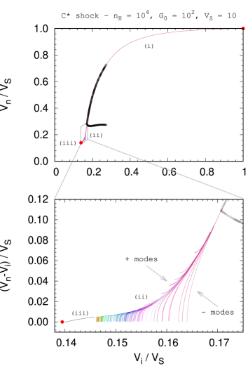
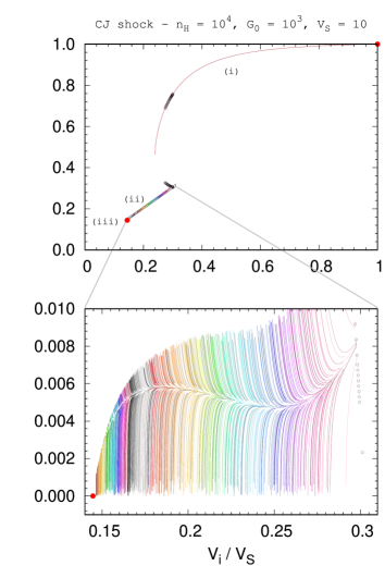
Figure 17: Phase diagrams of stationary shocks propagating at a speed of $10$ km s^-1 in a pre-shock medium with a density of $10^{4}$ $\,{\rm cm}^{-3}$, located at 0.6 mpc of the ionization front illuminated by an isotropic radiation field of $G_{0}=10^{2}$ (left) and $10^{3}$ (right). All other parameters are set to their standard values (see Table 1). The coloured curves correspond to the potential trajectories computed by the algorithm described in Appendix C. The true stationary solution connects the upstream and downstream trajectories (i) and (iii). This solution is bounded in the subsonic excursion (labelled ii) by the $+$ and $-$ modes (see main text). The top panels show the neutral and ion velocities relative to the velocity of the shock. The bottom panels are zooms of the top panels rotated to highlight the ion-neutral velocity drift. Initial and final kinematic states and potential jump conditions are indicated with red points and black circles, respectively.

Examples of CJ and C* shocks are shown in Fig. 17, which shows the typical evolutions of the neutral and ion velocities ($v_{n}$ and $v_{i}$) set by the steady-state evolution equations. The initial (pre-shock) and final (post-shock) kinematic states of the gas are indicated with red points. Assuming that their initial conditions are known, both the upstream and downstream supersonic parts (i and iii in Fig. 17) can be easily computed using the forward integration scheme of the Paris-Durham code. The real difficulty lies in calculating the subsonic excursion (part ii in Fig. 17) connecting the two, which corresponds to a unique solution among an infinite set of trajectories and which provides the initial conditions of the downstream flow. As shown by Roberge & Draine (1990), the solution can be found considering its two main properties: firstly, it necessarily ends at the downstream sonic point; secondly, it separates the phase diagram into two spaces where any perturbation on either the neutral or the ion velocities grows exponentially towards an unphysical solution (see Fig. 17). In the following we define as $+$ modes the trajectories leading to a change of sign of $dv_{n}/dz$ and as $-$ modes those leading to a change of sign of $dv_{i}/dz$.

With all these considerations, we built a convoluted algorithm based on a single precision parameter $\varepsilon$ which works as follows:

1. The upstream trajectory (i) is computed starting with the initial conditions of the flow. If the neutral fluid stays supersonic, the structure is a C-type shock and the computation is carried out as usual. If the neutral velocity gets close to the sound speed, the structure is either a CJ-type or C*-type shock and step 2 is activated.

2. The upstream trajectory is scanned to identify all the possible positions of an adiabatic jump (black points in Fig. 17), i.e. the positions where applying the Rankine-Hugoniot relations conserves the signs of $dv_{n}/dz$ and $dv_{i}/dz$ before and after the jump (see Roberge & Draine 1990 for more details). Potential trajectories are then computed, starting from different jump positions to find a $+$ and a $-$ mode. The jump positions are then refined by dichotomy such that the $+$ and $-$ modes converge towards the true stationary solution. This solution, identified when the relative velocities of the $+$ and $-$ modes differ by less than $\varepsilon$, is calculated as the average of the $+$ and $-$ trajectories. The flow then starts its subsonic excursion (ii).

3. During the subsonic excursion a shooting technique is applied where both the ions and neutral velocities are perturbed in order to identify again a $+$ and a $-$ mode. These perturbations are done in the $(v_{n},v_{i})$ phase space, in the direction perpendicular to the trajectory identified in step 2 as the true trajectory, with typical relative amplitudes smaller than $\varepsilon$. Once a $+$ and a $-$ modes are found, the true trajectory is computed as their average, up until the time where they differ by more than $\varepsilon$. At which point we start again step 3.

4. The previous algorithm stops either when $|v_{n}-v_{i}|/V_{S}\leqslant\varepsilon$ or $|v_{n}-c_{n}|/V_{S}\leqslant\varepsilon$, where $c_{n}$ is the sound speed and $V_{S}$ the shock speed. In the first case we assume that the neutrals and ions recouple ; this happens for instance in the bottom right panel of Fig. 17. In the second case, we estimate the distance $d$ left to reach the downstream sonic point and then extrapolate all variables (dynamical, thermal, and chemical) at twice that distance to continuously jump this point (see for instance the jump between parts ii and iii in the bottom left panel of Fig. 17). Once one of these two options is selected, the downstream trajectory (iii) is calculated by forward integration.

By default and for all the models presented in this paper, we use $\varepsilon=10^{-2}$, with the exception of Fig. 17 where a value of $10^{-3}$ is adopted. It is worth stressing that the success or failure of the algorithm is independent of $\varepsilon$. Changing this parameter impacts only the precision of the results and the computational time. Tests of this algorithm over the entire grid of models (see Sect. 3) shows that the procedure is stable and highly reliable with a success rate of about 97%. Most of the failures correspond to the parameter domain where stationary structures shift from C to C* shocks (i.e. at the interface between green and yellow panels in Fig. 4) and where computing the solution requires an adaptative selection of $\varepsilon$.

Appendix D Exploration of the parameter space

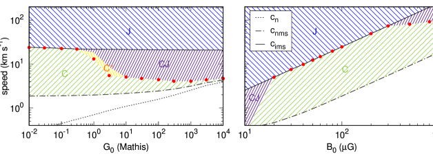
Figure 18: Neutral sound speed (dotted) and neutral (dot-dashed) and ion (solid) magnetosonic speeds as functions of the UV radiation field in a medium of density ${n_{\rm H}}=10^{2}$ $\,{\rm cm}^{-3}$ and a visible extinction $A_{V}^{0}=10^{-2}$ (upper left), and as functions of the transverse magnetic field intensity in a medium of density ${n_{\rm H}}=10^{4}$ $\,{\rm cm}^{-3}$ and $G_{0}=0$ (upper right). All other parameters are set to their standard values (see Table 1). The critical velocities above which C-type shocks cannot exist are shown with red points, while coloured areas highlight the range of velocities at which C- (green), C*- (yellow), CJ- (violet), and J-type (blue) shocks develop.

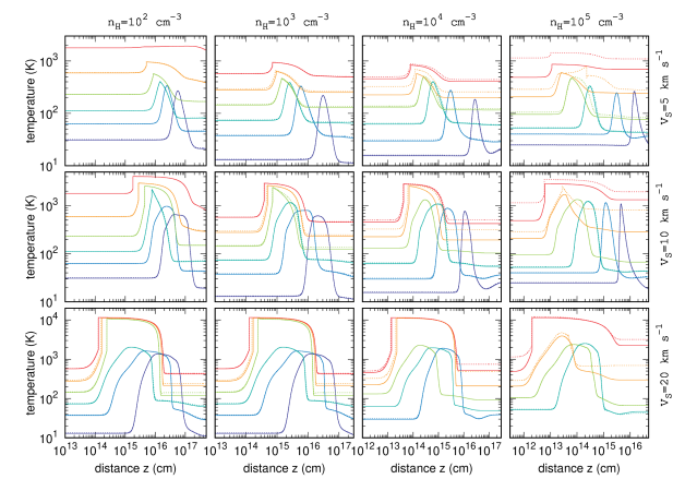
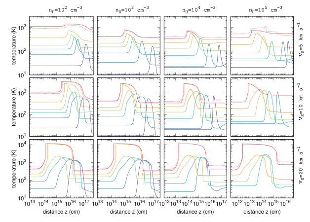
Figure 19: Temperature profiles of shocks from 5 to 20 km s^-1 (from top to bottom panels) propagating in media with density ranging from $10^{2}$ to $10^{5}$ $\,{\rm cm}^{-3}$ (from left to right panels) and illuminated by a UV radiation field ranging from $10^{-1}$ to $10^{4}$ (from colder to warmer pre-shock conditions on each panel), assuming a buffer visual extinction $A_{V}^{0}=10^{-2}$ (top 12 panels) and $10^{-1}$ (bottom 12 panels). All other parameters are set to their standard values (see Table 1). Models run with and without taking the UV pumping of the rovibrational levels of $\rm H_{2}$ into account are shown in dashed and solid curves, respectively.

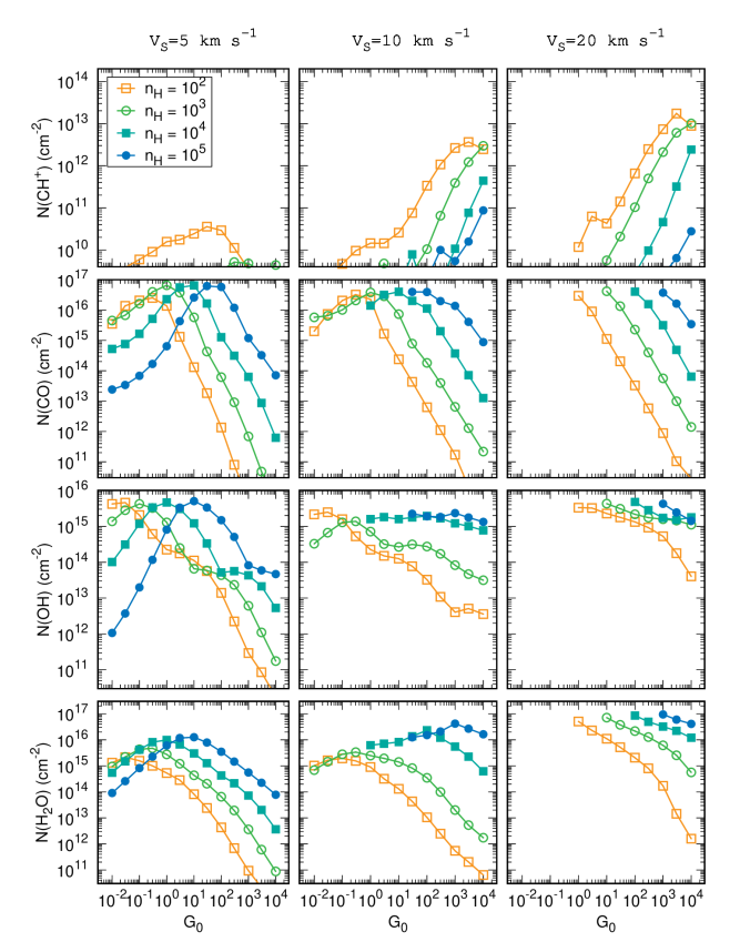
Figure 20: Same as Fig. 11 assuming a buffer visual extinction $A_{V}^{0}=1$.

To be exhaustive, we regroup a few additional figures and results that complement those already discussed in the main text of the paper.

Fig. 18 shows the domains of existence of C, C*, CJ, and J-type shocks in irradiated diffuse interstellar media (left panel) and in dense and totally shielded environments (right panel). We recall that if no radiation field is considered ($G_{0}=0$), as it is the case in the right panel of Fig. 18, adsorption and desorption processes are switched off for the computation of the pre-shock properties during which we adopt the chemical composition of grain mantles given in Table 2 of Flower & Pineau des Forêts (2003).

We find that the domain of existence of C-type shocks considerably reduces in diffuse environments compared with that computed in dense clouds with similar irradiation conditions (see Fig. 3). Interestingly, C-type shocks with velocity larger than 13 km s^-1 do not exist in typical diffuse clouds of density ${n_{\rm H}}=10^{2}$ $\,{\rm cm}^{-3}$ with mild irradiation conditions ($G_{0}$=1), a limit that quickly drops with the strength of the radiation field. In these conditions, C-type shocks are replaced by CJ-type shocks, which clearly become a dominant dissipative structure in highly irradiated diffuse gas. The limits inferred in completely shielded environments are found to be in good agreement with those derived with the previous version of the Paris-Durham shock code (Cabrit et al. 2004), except at low magnetization where we highlight a new domain of existence of CJ-type shocks.

As a complement to Fig. 4, we represent in Fig. 19 the temperature profiles obtained in 288 models of molecular shocks covering roughly the entire grid of parameters explored in this work. As described in the main text, the external UV radiation field reduces the size of the shock, which induces an increase of the temperature peak and reveals the entwinement of the impacts of radiative and mechanical energies on the thermal evolution of the gas. We find that low velocity shocks ($V_{S}\leqslant 5$ km s^-1) propagating in highly illuminated environments ($G_{0}=10^{4}$) have almost no impact on the temperature of the gas. This result unveils the limit at which the dissipation of mechanical energy is virtually undetectable compared to the amount of radiative energy locally reprocessed by interstellar matter.

In addition to Fig. 11, we finally indicate in Fig. 20 the column densities of $\rm CH^{+}$, CO, OH, and H₂O computed across molecular shocks in well-shielded environments ($A_{V}^{0}=1$). The results obtained in these conditions are found to be similar to those obtained at lower visual extinction for lower irradiation conditions (Fig. 11). In particular, the strong increase of $\rm CH^{+}$ column densities and the strong decrease of those of CO, OH, and H₂O in highly irradiated environments is a general result that does not depend on the extinction considered.