Physical properties of SDSS satellite galaxies in projected phase-space

Abstract

We investigate how environment affects satellite galaxies using their location within the projected phase-space of their host haloes from the Wang et al.’s group catalogue. Using the Yonsei Zoom in Cluster Simulations, we derive zones of constant mean infall time $\overline{\rm T}$_inf in projected phase-space, and catalogue in which zone each observed galaxy falls. Within each zone we compute the mean observed galaxy properties including specific star formation rate, luminosity-weighted age, stellar metallicity and [$\alpha$/Fe] abundance ratio. By comparing galaxies in different zones, we inspect how shifting the mean infall time from recent infallers ($\overline{\rm T}$${}_{\rm inf}~{}<$ 3 Gyr) to ancient infallers ($\overline{\rm T}$${}_{\rm{inf}}>$ 5 Gyr) impacts galaxy properties at fixed stellar and halo mass. Ancient infallers are more quenched, and the impact of environmental quenching is visible down to low host masses ($\leq$ group masses). Meanwhile, the quenching of recent infallers is weakly dependent on host mass, indicating they have yet to respond strongly to their current environment. [$\alpha$/Fe] and especially metallicity are less dependent on host mass, but show a dependence on $\overline{\rm T}$_inf. We discuss these results in the context of longer exposure times for ancient infallers to environmental effects, which grow more efficient in hosts with a deeper potential well and a denser intracluster medium. We also compare our satellites with a control field sample, and find that even the most recent infallers ($\overline{\rm T}$_inf < 2 Gyr) are more quenched than field galaxies, in particular for cluster mass hosts. This supports the role of pre-processing and/or faster quenching in satellites.

1 Introduction

It is now well accepted that environmental effects are acting to transform galaxies in their morphology (Dressler 1980), colours (e.g. Tanaka et al. 2004, Weinmann et al. 2006, Weinmann et al. 2009, Vulcani et al. 2015), atomic gas content (Giovavelli & Haynes 1985, Chung et al. 2009, Jaffé et al. 2015, Jaffé et al. 2018), and their star formation rates (e.g. Hashimoto et al. 1998, Dominínguez et al. 2002, Gómez et al. 2003, Kauffmann et al. 2004, Poggianti et al. 2008, Balogh et al. 2011, McGee et al. 2011, Hou et al. 2013, Lin et al. 2014, Mok et al. 2014, Davies et al. 2016, Lofthouse et al. 2017). A variety of mechanisms whose efficiency is environmentally dependent may be responsible for these transformations including: ram pressure stripping (Gunn & Gott 1972), starvation (Larson et al. 1980, Balogh et al. 2000, Bekki 2009), harassment (Moore et al. 1996, Moore et al. 1998, Gnedin et al. 2004, Smith et al. 2010, 2012, 2015), and galaxy-galaxy mergers (Barnes & Hernquist 1996). Until fairly recently, many studies of galaxy environment have often focused on the densest environments such as clusters. However, it is now clear that the transformations can begin to occur in lower density environments, and that galaxy colours and star formation rates systematically vary with the density of their environment over a density range from voids, to filaments and walls, through groups, all the way up to cluster densities (Cybulski et al. 2014). Furthermore, thanks to the hierarchical manner in which structure growth occurs, many galaxies which are members of clusters today may have previously spent time in a group environment, and suffered group pre-processing (Zabludoff & Mulchaey 1998, Balogh et al. 2000, De Lucia et al. 2012, Hoyle et al. 2012, Vijayaraghavan & Ricker 2013, Hirschmann et al. 2014), meaning they have experienced both group and cluster environmental effects. Recent studies have in fact revealed that galaxies in groups are more deficient in atomic gas (Brown et al. 2017). By stacking X-ray images of individual galaxies, Anderson et al. (2013, 2015) have revealed that on average all galaxies with masses down to $\sim$10^10.5 M_⊙ are surrounded by an extended X-ray emitting ionised gas that could give rise to starvation or ram pressure.

When trying to understand the impact of environment on galaxies, it is crucial to first control for the effect of galaxy mass. This is because it is generally accepted that ‘mass quenching’ is a crucial process controlling galaxy evolution. It can be broadly understood in terms of the ‘halo quenching’ process (Gabor & Davé 2015), where the gas in haloes more massive than 10¹² M_⊙ is hindered from cooling as it becomes shock-heated (Birnboim & Dekel 2003; Dekel & Birnboim 2006). However, galaxy simulations tend to agree that AGN feedback is an additional yet necessary process to keep galaxies quenched over long time-scales (e.g. Granato et al. 2004, Bower et al. 2006). Galaxy mergers (Hopkins et al. 2006) and/or disk instabilities (Dekel et al. 2009) have also been recognized as further quenching mechanisms. The effects of all these processes scale with galaxy mass, and thus must be disentangled from the effects of environment. This was clearly demonstrated in Peng et al. (2010), who showed that galaxy colour is a function of both galaxy mass and local environmental density, and by Pasquali et al. (2010), who found that satellite stellar age and metallicity depend on both galaxy mass and host halo mass.

When a galaxy first enters an environment of different density (e.g. a field galaxy falls into the cluster), clearly we should expect it to take a finite time for its new environment to take effect. Recently, the time it takes for galaxies to be fully quenched has been a subject of much discussion in the literature, with the general conclusion that the transformation takes place over several gigayears (cf. De Lucia et al. 2012, Wetzel et al. 2013, Oman & Hudson 2016, Hirschmann et al. 2014). Such long time scales for environmentally-induced quenching are supported also by the observations that the relation between the element abundance ratio [$\alpha$/Fe] and stellar mass is to a large extent independent of galaxy hierarchy and halo mass, as we find in Gallazzi et al. (2018, in prep). Simply measuring the local environmental density may not provide all the relevant information, as galaxy properties would be expected to vary as a function of time spent in that environment. In other words, at fixed environmental density, there will be some galaxies that are very recent newcomers to that environment and whose properties may be much more shaped by their previous environment. This issue may be more severe in regions where there has been rapid recent growth, causing the environment to be flooded by recent infallers. Ideally, we would greatly benefit from being able to control for the effect of infall time - the time at which an object joined its environment.

One promising tool that may allow us to have some handle on the infall times of satellites into their current host is through the use of phase-space diagrams, combining cluster-centric (or group-centric) velocity with cluster-centric (or group-centric) radius. As a function of distance alone, the infall time is poorly constrained. This is because, in $\Lambda$CDM, typically the orbits of an infalling substructure are very plunging and eccentric (Gill et al. 2005, Wetzel 2011). As a result, at a fixed radius inside a cluster there may be objects falling in for the first time, combined with objects that have been orbiting within the cluster for many gigayears, creating a wide distribution of infall times. As a consequence, any correlation that can be recognized between mean infall time and cluster-centric distance suffers from a large scatter (see Gao et al. 2004, De Lucia et al. 2012). However, when cluster-centric distance is combined with cluster-centric velocity (e.g. a phase-space diagram), recent infallers to the cluster tend to shift to higher velocities than objects that have been in the cluster for some time. Thus different regions of phase-space tend to be dominated by objects with a narrower range of infall time. In a 3D phase-space diagram (using the 3D cluster-centric radius and 3D cluster-centric velocity), different infall time populations separate quite neatly (e.g. the left panel of Figure 2 of Rhee et al. 2017). Nevertheless, when we consider observable quantities (line of sight velocity and projected radius from the cluster), there is often much more mixing of objects with differing infall times as a result of projection effects. Despite this, the shape of the infall time distribution systematically varies with location in projected phase-space (Oman & Hudson 2016, see for example Figure 5 of Rhee 2017).

A number of authors have used phase-space diagrams as tools to better understand galaxy evolution, including Mahajan et al. (2011, star formation), Muzzin et al. (2014, high redshift quenching), Hernández-Fernández et al. (2014) and Jaffé et al. (2015, gas fractions and ram pressure), Oman & Hudson (2016, quenching timescales), Yoon et al. (2017, ram pressure in Virgo), Jaffé et al. (2018, jelly fish galaxies undergoing ram pressure). In this paper, in order to take the next step forward, we will attempt to control for the effect of galaxy mass and also galaxy environment, while simultaneously controlling for the effect of infall time of the galaxies into their environment using projected phase-space diagrams. Since it is impossible to assign each galaxy an infall time, due to the mixing of infall times in each region of a projected phase-space diagram, we will theoretically define various zones in phase-space such that we can assume, by comparison with cosmological simulations of clusters and groups, that the mean of the infall time distribution is changing systematically with zone. Then, by comparing the population of galaxies in each zone, we can study how galaxy mean, observed properties change as their mean infall time shifts with zone. Our sample includes satellite galaxies with masses varying from dwarfs to giants, and host haloes with masses varying from large galaxies up to massive clusters. By spectral fitting, we can study multiple properties of our galaxies including luminosity-weighted age, specific star formation rate, metallicity and $\alpha$-abundances. Indeed this paper represents the first attempt to investigate how all of these properties vary as a function of galaxy mass, host mass while deliberately shifting the mean infall time of the population in a systematic way.

In Section 2 we describe the group catalogue from which our host and satellite samples are drawn, describe how spectral fitting is conducted, and summarise the working sample. In Section 3 we describe the cosmological simulations that we compare with, and explain how we choose the different zones in phase-space. In Section 4 we present our results for how galaxy properties vary with zone and compare our sample of satellite galaxies with a field sample. We discuss and interpret our results in Section 5, compute quenching time-scales as a function of stellar and host mass, and comment on possible indications of pre-processing. Finally, in Section 6 we summarise our results and draw conclusions.

2 Data

2.1 Assessing galaxy environment

We used the galaxy group catalogue drawn from the Sloan Digital Sky Survey Data Release 7 (SDSS DR7) by Wang et al. (2014) following the procedure of Yang et al. (2007). Briefly, the adaptive halo-based group finder developed by Yang et al. (2005) was applied to all galaxies in the Main Galaxy Sample of the New York University Value-Added Galaxy Catalogue (Blanton et al. 2005) for DR7 (Abazajian et al. 2009), which have an extinction corrected apparent magnitude brighter than $r=$ 17.72 mag, and are in the redshift range 0.01 $\leq z\leq$ 0.20 with a redshift completeness C${}_{z}>$ 0.7. This algorithm employs the traditional firedns-of-firends method with small linking lengths in redshift space to sort galaxies into tentative groups and estimate the groups’ characteristic stellar mass and luminosity. In the first iteration, the adaptive halo-based group finder applies a constant mass-to-light ratio of 500 $h$M_⊙/L_⊙ to estimate a tentative halo mass for each group. This mass is then used to evaluate the size and velocity dispersion of the halo embedding the group, which in turn are utilized to define group membership in redshift space. At this point a new iteration begins, whereby the group characteristic luminosity and stellar mass are converted into halo mass using the halo occupation model of Yang et al. (2005). This procedure is repeated until no more changes occur in the group membership.

When applied to SDSS DR7, the adaptive halo-based group finder delivers three group samples: sample I, which relies only on those galaxies (593,736) with a spectroscopic redshift measured by SDSS; sample II, which extends the previous one by 3,115 galaxies with SDSS photometry whose redshifts are known from alternative surveys; sample III, containing an additional 36,602 galaxies without redshift because of fiber collision, but which were assigned the redshift of their closest neighbour (cf. Zehavi et al. 2002). In each group sample, galaxies are distinguished between centrals (the most massive group members in terms of stellar mass M_⋆), and satellites (all other group members less massive than their group central). Stellar masses have been calculated using the relations between stellar mass-to-light ratio and colour from Bell et al. (2003), while the dark matter masses M_h associated with the host groups have been estimated on the basis of the ranking of both the group total characteristic luminosity and the group total characteristic stellar mass (cf. Yang et al. 2007 for more details). The two available M_h values are reasonably consistent with each other (with an average scatter decreasing from 0.1 dex at the low-mass end to 0.05 dex at the massive end), although More et al. (2011) showed that stellar mass constrains M_h better than luminosity. The method of Yang et al. (2007) is able to assign a value of M_h only to galaxy groups more massive than $\sim$10¹² M${}_{\sun}h^{-1}$ and containing at least one member with ^0.1M_r - 5log$h\leq$ -19.5 mag, where ^0.1M_r is the galaxy absolute magnitude in $r$ band corrected to $z=$ 0.1. For smaller haloes, M_h has been extrapolated from the relations between the luminosity/stellar mass of central galaxies and the halo mass of their host groups, thus reaching a limiting M_h of $\sim$10¹¹ M${}_{\sun}h^{-1}$ (cf. Yang, Mo & van den Bosch 2008). As shown by Yang et al. (2007), the typical uncertainty on M_h varies between $\sim$ 0.35 dex in the range M_h = 10^13.5 - 10¹⁴ M${}_{\odot}h^{-1}$ and $\sim$ 0.2 dex at lower and higher halo masses.

For our analysis of the observed galaxy properties in projected phase-space we made use of sample II, and halo masses derived from the group characteristic stellar mass. From sample II we extracted all galaxy groups with at least 4 members (the central galaxy plus three satellites). We choose this minimum number of members in order to ensure that our groups can truly be considered groups and not simply pairs of interacting galaxies. Groups with 4 members may have a less well determined centre and thus the projected cluster-centric distances of their satellites may be more uncertain. This mostly concerns the lower M_h haloes (10¹² - 10¹³ M${}_{\sun}h^{-1}$) where the fraction of satellites living in groups with 4 members is 44$\%$ for 9 $\leq$ log(M_⋆ M${}_{\sun}h^{-2})<$ 10, 59$\%$ for 10 $\leq$ log(M_⋆ M${}_{\sun}h^{-2})<$ 10.5 and 72$\%$ at higher stellar masses. Nevertheless, we believe that increasing the galaxy statistics by combining all groups in the low M_h range partially mitigates the effect of an uncertain group centre on our results, and we will show that trends with phase-space zone still persist.

We used the spectroscopic redshifts of the satellites belonging to the same group to derive their line-of-sight velocities, and to compute the velocity dispersion along the line of sight ($\sigma$) of their group using the standard unbiased estimator for the variance. We also determined the peculiar line-of-sight velocity of each satellite, $|\Delta{\rm V}|$, as the absolute value of the difference between its line-of-sight velocity and the mean of the satellite line-of-sight velocities. The projected distance of each satellite from the luminosity weighted centre of its host group is given in sample II as R_proj in kpc $h^{-1}$. In addition, we calculated the group virial radius R₂₀₀ (at which the average group density is 200 times higher than the critical density) using the relation (cf. Yang et al. 2007):

$${\rm R_{\rm 200}[kpc~{}h^{-1}]=\frac{258.1\times(M_{\rm h}/10^{12})^{1/3}\times(\Omega_{\rm m}/0.25)^{1/3}}{(1+z_{\rm g})}}$$ (1)

where we assumed $\Omega_{\rm m}$ = 0.272 to be consistent with the simulations described below. This allows us to normalise each satellite’s projected group-centric distance by R₂₀₀ (i.e R_proj/R₂₀₀). Combining this parameter with $|\Delta V|$/$\sigma$ defines the position of each satellite in the projected phase-space diagram of its host group. We note that Eq.(1) well reproduces the virial radius of the simulated clusters described in Sect. 3. As we only ever see a component of a galaxy’s true velocity, or true group-centric distance, down our line-of-sight, the projected position has to be considered a lower limit on the true 3D position (based on the galaxy’s 3D group-centric distance and velocity). We restrict our sample to only include satellites that fall within their host’s virial radius in projected distance. By only considering satellites that are quite close to their host, we can expect stronger environmental effects. Also, in this way we can limit the contamination from interlopers (galaxies that are not associated with the cluster but are merely projected onto it) on our results. Beyond one virial radius, interlopers begin to dominate over the cluster population, but inside the zones in phase-space that we consider (see Sect. 3.1), the interloper fraction is never larger than 40$\%$. In fact, 92$\%$ of the group/cluster population is found in zone $\leq$ 4 where the fraction of interlopers is $<$ 22$\%$ and the cluster population dominates.

Since sample II is not volume limited, we had to correct our basic sample for Malmquist bias, which is responsible for an artificial increase of the average luminosity (and M_⋆) of galaxies with redshift in our data. Such an effect is more critical for satellites which, at fixed M_h, cover a wider luminosity/mass distribution. We thus weighted each galaxy in our analysis by 1/V_max, where V_max is the comoving volume corresponding to the comoving distance at which that galaxy would still have satisfied the selection criteria of the group catalogue.

2.2 Stellar populations

We matched our basic sample with the catalogue of stellar ages, metallicities and [$\alpha$/Fe] values of SDSS DR7 galaxies by Gallazzi et al. (2018 in prep). The stellar population parameters were computed following the same methodology as in Gallazzi et al. (2005). Briefly, the strength of the spectral indices D4000_n, H$\beta$, H$\delta_{A}$ $+$ H$\gamma_{A}$, [MgFe]^′ and [Mg₂Fe] is compared with synthetic spectra built from Bruzual $\&$ Charlot (2003) SSP models convolved with a large Monte Carlo library of star-formation histories and metallicities. This produces probability distribution functions (PDFs) of r-band luminosity-weighted age and stellar metallicity, from which we can derive median values and their corresponding uncertainty based on half of the (84^th - 16^th) percentile range.

For what concerns the [$\alpha$/Fe] abundance ratios, they were estimated following the approach of Gallazzi et al. (2006). For each galaxy, the index ratio Mgb/$<{\rm Fe}>$ (where $<{\rm Fe}>$ is the average of the Fe5270 and Fe5335 index strengths) is computed from the observed spectrum and also from the solar-scaled model that best fits the aforementioned spectral indices (all being independent of [$\alpha$/Fe]). The difference between data and model (denoted as $\Delta$Mgb/$<{\rm Fe}>$) can be considered as an excess of [$\alpha$/Fe] with respect to the solar value. Specifically, Gallazzi et al. (2018, in prep) calculate the full PDF of $\Delta$Mgb/$<{\rm Fe}>$ from which we then estimate a median value and its related uncertainty as half of the (84^th - 16^th) percentile range. Finally, Gallazzi et al. calibrate the relation between $\Delta$Mgb/$<{\rm Fe}>$ and [$\alpha$/Fe] as a function of age and stellar metallicity using the stellar population models of Thomas et al. (2003, 2004). It thus becomes possible to assign an [$\alpha$/Fe] value to each galaxy in the sample on the basis of its best-fit age, stellar metallicity and computed $\Delta$Mgb/$<{\rm Fe}>$.

When matching the satellites of our basic sample with the catalogue of stellar parameters, we kept only those galaxies with an estimated age and whose median spectral S/N per pixel is equal or larger than 20. This ensures, as shown by Gallazzi et al. (2005), an uncertainty on stellar age and metallicity of $\sol$ 0.2 and 0.3 dex respectively. The cut in S/N introduces a bias toward brighter galaxies or galaxies with deeper absorptions that may affect our results. In order to correct for incompleteness at fixed stellar mass we apply to each galaxy a weight $w_{SN}$ as computed in Gallazzi et al (2018, in prep). This weight $w_{SN}$ is calculated in bins of stellar mass (0.1 dex width) and absolute $(g-r)^{z=0.1}$ Petrosian colour (0.2 mag width) taken as model-independent proxy for stellar population properties. It is defined as the number ratio in each bin between the galaxies in the parent sample and those with spectral S/N $>$ 20. To avoid overweighing bins in which the statistic is low and $w_{SN}$ uncertain, we exclude bins in which high-S/N galaxies are fewer than 10 and less than 10$\%$ of the total. These are a negligible fraction of galaxies and does not impact our conclusions.

In this way, we select 20928 satellites which make up our final working sample. We retrieved the median, 16^th and 84^th percentile values of their global, specific star formation rates (sSFR_gl) from the catalogue by Brinchmann et al. (2004). We computed the uncertainty on the median sSFR_gl as half of the (84^th - 16^th) percentile range.

Figure 1: The weighted (solid line) and unweighted (dotted line) distribution of our working sample in the properties analyzed below: global specific SFR, luminosity-weighted stellar age, stellar metallicity and [$\alpha$/Fe] ratio.

2.3 Characterizing the working sample

The satellites of our working sample span a redshift range between $z$ = 0.01 and $z$ = 0.2, peaking at $z\simeq$ 0.072 and with 90$\%$ of the galaxies below $z\simeq$ 0.15. They are distributed in stellar mass between 10⁹ and $\sim$10^11.5 M${}_{\odot}h^{-2}$, and populate a wide range of environments, with host haloes varying in mass between 10¹² and 10¹⁵ M${}_{\odot}h^{-1}$. The solid line in Fig. 1 shows their distribution weighted by (1/V_max $\times$ $w_{SN}$) in global specific SFR (sSFR_gl), luminosity-weighted stellar age (Age_L), stellar metallicity (log (Z/Z_⊙)) and [$\alpha$/Fe] abundance ratio. About 70$\%$ of the satellites in our working sample are passive with log(sSFR_gl yr^-1) $\sol$ -11 and luminosity-weighted stellar age older than $\sim$4 Gyr. We note that half of the working sample has solar or above solar metallicity, while the majority of satellites have [$\alpha$/Fe] ratios between solar and 0.5 dex. For comparison, we also trace in Fig. 1 the unweighted distributions of our working sample (dotted lines). They show how our weighing scheme shifts the satellites distribution towards higher sSFR_gl and younger Age_L, lower stellar metallicity and [$\alpha$/Fe] ratio.

For a first investigation of the projected phase-space populated by our working sample, we select satellites in the stellar mass range 10⁹ M${}_{\odot}h^{-2}\leq$ M${}_{\star}\leq$ 10¹⁰ M${}_{\odot}h^{-2}$ residing in host haloes in the mass interval 10¹³ M${}_{\odot}h^{-1}\leq$ M${}_{\rm h}\leq$ 10¹⁵ M${}_{\odot}h^{-1}$, since Pasquali et al. (2010) showed their properties to be most sensitive to environment. Figure 2 presents the distribution of the peculiar velocities of these satellites, normalized by their host group velocity dispersion, as a function of their projected distance from the luminosity-weighted centre of their group, normalized by the group virial radius R₂₀₀. Such distribution follows the typical trumpet shape. This arises because as galaxies with low angular momentum move closer to the cluster centre, they tend to gain velocity as they approach pericentre. In order to highlight the trumpet-shape, we overlay the plot with solid lines which trace out the caustic profile $\Delta V/\sigma$ $\times$ R${}_{\rm proj}/$R${}_{\rm 200}=\pm$ 0.6.

Figure 2: The distribution of satellites with 10⁹ M${}_{\odot}h^{-2}\leq$ M${}_{\star}\leq$ 10¹⁰ M${}_{\odot}h^{-2}$ and 10¹³ M${}_{\odot}h^{-1}\leq$ M${}_{\rm h}\leq$ 10¹⁵ M${}_{\odot}h^{-1}$ in projected phase-space. The solid lines are the caustic profile $\Delta V/\sigma$ $\times$ R${}_{\rm proj}/$R${}_{\rm 200}=\pm$ 0.6.

In Fig. 3 we present the projected phase-space plane of Fig. 2 colour-coded on the basis of the fraction of passive satellites and the fraction of old and young satellites. For each galaxy we select its 100 closest neighbours in the R_proj/R₂₀₀ - $\Delta$V/$\sigma$ plane, and separate them between passive and star-forming using the separation line derived by Oman & Hudson (2016) and according to their observed sSFR and stellar mass. We then compute the fraction of passive satellites, weighted by (1/V_max $\times$ $w_{SN}$), as a function of R${}_{\rm proj}/$R₂₀₀ and $\Delta V/\sigma$ (top panel). We also use the luminosity-weighted stellar age to distinguish these 100 closest neighbours between young (Age${}_{\rm L}<$ 3 Gyr) and old (Age${}_{\rm L}>$ 7 Gyr) and calculate their corresponding weighted fraction (see middle and bottom panels, respectively). Fig. 3 reveals an overall decrease in the fraction of passive or older satellites with projected cluster-centric distance, matched by an increase in the fraction of younger satellites. The more actively star-forming and younger satellites are mostly located at the virial radius, but also at $|\Delta V|/\sigma\sog$ 2. Quiescent and older satellites preferentially populate the inner region of their host environment. These trends with R${}_{\rm proj}/$R₂₀₀ essentially occur at any fixed value of $|\Delta V|/\sigma$.

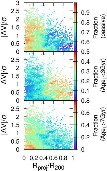
Figure 3: The observed distribution of the fraction of passive satellites (top panel), the fraction of satellites younger than 3 Gyr (middle panel) and older than 7 Gyr (bottom panel) across projected phase-space. These are computed for satellites in our working sample in the range 10⁹ M${}_{\odot}h^{-2}\leq$ M${}_{\star}\leq$ 10¹⁰ M${}_{\odot}h^{-2}$, residing in host haloes with 10¹³ M${}_{\odot}h^{-1}\leq$ M${}_{\rm h}\leq$ 10¹⁵ M${}_{\odot}h^{-1}$.

3 Galaxy cluster simulations

In order to improve on the scatter in Fig. 3 and better understand its trends, we require some knowledge of the times at which our galaxies first fell into their current environment. For this, we must compare our observations to a set of hydrodynamic zoom-in simulations of galaxy clusters. Here we provide a brief summary of the hydrodynamical simulations (refereed to as YZiCS), but a full description is available in Choi $\&$ Yi (2017). We ran cosmological hydrodynamic zoom-in simulations using the adaptive mesh refinement code ramses (Teyssier 2002). We first run a large volume cube of side length 200 Mpc h^-1 using dark matter particles only, within the WMAP7 cosmology (Komatsu et al. 2011): $\Omega_{\rm{M}}$ = 0.272, $\Omega_{\Lambda}$ = 0.728 and H₀ = 70.4 km s^-1 Mpc^-1, $\sigma_{8}$ = 0.809, and n = 0.963. We then select 15 high density regions in the cosmological volume and perform zoom-in simulations, this time including hydrodynamic recipes. The zoom-in region contains all particles within 3 viral radii of a cluster at z = 0. The mass range of our clusters varies from 9.2$\times$10¹⁴ M_⊙ to 5.3 $\times$ 10¹³ M_⊙. A summary of their properties can be found in Table 1 of Rhee et al. (2017). The minimum cell size is 760 pc h^-1 and 8$\times$10⁷ M_⊙ in dark matter particle mass. Halo-finding and tree-building were conducted using the AdaptaHOP method (Aubert et al. 2004). Each snapshot is only approximately 75 Myr apart, which greatly aids this process. To ensure we have a complete halo mass function, and to reduce numerical effects, we discard all subhaloes whose peak mass is lower than 3 $\times$10¹⁰ M_⊙ from our analysis. With this mass cut, all haloes can be considered as a proxy for a galaxy, and, even in the worst case, we can follow halo mass loss down to 3$\%$ of the peak mass. We have adopted the baryon prescriptions of Dubois et al. (2012) including gas cooling, star formation, stellar and AGN feedback, and were able to reproduce the basic properties of observed $z\sim$0 galaxies to the same degree as in the Horizon-AGN simulations (Dubois et al. 2014).

In order to compare our simulations with the data, we compute a projected phase-space diagram for each individual cluster, considering 1000 line of sights (increasing this number by a factor of five introduces negligible differences, cf. Rhee et al. 2017). We then combine all the cluster phase-space planes together so that each of them has equal weight in the final projected phase-space in order to avoid biases due to varying numbers of cluster members.

To this set of simulations we add data extracted from a suite of 8 zoom-in cosmological simulations of clusters. These simulations are fully described in Warnick $\&$ Knebe (2006). In short, these are N-body simulations that were performed with the adaptive mesh refinement code mlpam (Knebe, Green $\&$ Binney 2001). The simulations are dark-matter only but the resolution is roughly comparable with the mass and spatial resolution of the YZICS simulations. Each dark matter particle has a mass of $\sim$1.6$\times$10⁸ M_⊙, the highest spatial resolution is $\sim$2 kpc, and the 8 clusters are in the mass range 1–3$\times$10¹⁴ M_⊙. Smith et al. (2015) systematically measured the orbital parameters (eccentricity and pericentre distance of the most recent orbit) for all surviving subhaloes within these cluster simulations (see blue shading in Fig. 10 of Smith et al. 2015). For convenience, we use this existing data set to look at how these orbital parameters vary across phase-space, stacking together all clusters into a single phase-space diagram. We exclude all objects which are yet to reach a first pericentre passage as their orbital parameters are not yet defined.

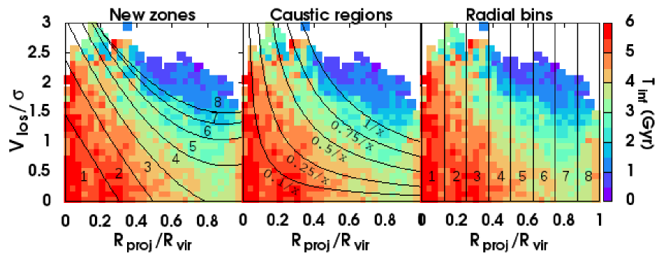
Figure 4: The distribution of infall time, T_inf, in Gyr across the projected phase-space, computed by averaging the simulated galaxies in 2D bins. Left-hand panel: The family of curves defined by Eq. (3) and Eq. (4) is plotted with solid black lines, and the zones in which these curves split the projected phase-space are numbered. Middle panel: several representative caustic profiles, which follow the analytical expression $y=c/x$ with $y=|\Delta V|/\sigma$ and $x$ = R_proj/R_vir. Right-hand panel: the projected phase-space is dissected among 8 equally wide radial bins.

3.1 Discretizing phase-space

Caustic profiles (as shown in Fig. 2) have usually been used in the literature to separate kinematically different galaxy populations in phase-space, which were accreted onto their parent halo at different times (e.g. Mamon et al. 2004; Gill et al. 2005; Mahajan et al. 2011; Haines et al. 2012). In particular, Noble et al. (2013, 2016) introduced plots of galaxy observed properties as a function of caustic profile defined as $|\Delta V|$/$\sigma$ $\times$ R_proj/R₂₀₀, as different values of this parameter generally correspond to different infall times.

We check how closely caustic profiles trace the accretion history of a massive halo by computing the mean infall time, T_inf, in two-dimensional bins across the projected phase-space of the satellites in the hydrodynamic simulations set. T_inf is defined as the time since a galaxy crossed for the first time the virial radius of the main progenitor of its present-day host environment. The result is shown in Fig. 4, where the distribution of simulated satellites in phase-space is colour-coded on the basis of their mean T_inf (Gyr) computed in 2D bins. Galaxies that have not yet entered the cluster are excluded from this plot as they do not have a T_inf value, and thus interlopers are also excluded. As already pointed out by Rhee et al. (2017), T_inf decreases with both increasing R_proj/R_vir and $|\Delta V|$/$\sigma$, so that the most recently accreted ($\sim$1.5 Gyr ago) galaxies have a relatively high peculiar velocity and are found in the outskirts of their host halo, while the satellites that fell in earliest ($\sim$5.5 Gyr ago) typically have a smaller peculiar velocity and a smaller, projected cluster-centric distance. The comparison of Fig. 4 with Fig. 3 highlights a correspondence between the distribution of satellite fractions and the distribution of T_inf across projected phase-space. Also, the vertical stripes of constant fraction value in Fig. 3 are reminiscent of the zones of constant T_inf in Fig. 4, although they appear less pronounced, possibly because of the contribution from interlopers that are excluded in Fig. 4. Such a similarity points to more quiescent satellites with the stellar populations that appear old today having been accreted earlier onto their present-day host halo.

In the middle panel of Fig. 4 we over-plot a few representative caustic profiles, whose analytical form is $y=c/x$, where $y=|\Delta V|/\sigma$, $x$ = R_proj/R_vir and $c$ a numerical coefficient which varies across the projected phase-space. In particular, we define the following set of caustic profiles:

$$\begin{split}1:y&=0.10/x\\ 2:y&=0.25/x\\ 3:y&=0.50/x\\ 4:y&=0.75/x\\ 5:y&=1.00/x\\ 6:y&>1.00/x\end{split}$$ (2)

We also split the projected phase-space in 8 equal width radial bins in the right-hand side panel of Fig. 4 (we do so because it is common use in the literature to show how satellite properties vary as a function of cluster-centric distance). It is clear that both caustic profiles and radial bins do not well match the shape of the infall time distribution. We thus replace them with a family of quadratic curves which are customised to split up the projected phase-space into eight new zones within 1 R_vir, which follow the infall time distribution, as plotted in the left-hand side panel of Fig. 4. Each curve has the analytical form:

$$|\Delta V|/\sigma=a{\rm(R_{\rm proj}/R_{\rm vir})}^{2}+b{\rm(R_{\rm proj}/R_{\rm vir})}+c$$ (3)

where the coefficients $a$, $b$ and $c$ are expressed as a function of $p$, an integer number running between 1 and 7:

$$\begin{split}a&=0.022p^{3}-0.512p^{2}+3.287p-2.786\\ b&=0.184p^{2}-1.494p-3.5\\ c&=-0.108p^{2}+1.249p+0.314\end{split}$$ (4)

For example, $p$ = 1 gives the dividing line between zone 1 and zone 2. In Fig. 5 we present the distribution in projected phase-space of the number density of the simulated satellites. The curves defined by Eq. (3) and Eq. (4) are overlaid and the new zones numbered. We can see that the average number density decreases with increasing zone number as expected, but is still high to statistically justify the definition of zones $\geq$ 5.

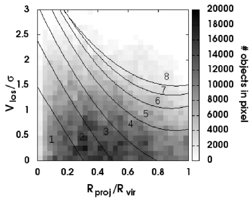
Figure 5: The distribution of the number density of the simulated galaxies across projected phase-space. The curves defined by Eq. (3) and Eq. (4) are overplotted as black lines, and the zones which they separate are labelled with a zone number.

Table 1: The average infall time $\overline{\rm T}$_inf and its associated standard deviation ($\sigma$($\overline{\rm T}$_inf)) as derived for the 8 new zones, the 6 caustic regions as well as the 8 equally wide radial bins drawn in Fig. 4. We also list the first and third quartiles of the T_inf distribution within each of these areas.

Zones	First	$\overline{\rm T}$inf	Third	$\sigma$($\overline{\rm T}$inf)
	quartile		quartile
	(Gyr)	(Gyr)	(Gyr)	(Gyr)
1	3.41	5.42	7.13	2.51
2	3.02	5.18	7.13	2.60
3	2.33	4.50	6.39	2.57
4	2.10	3.89	5.66	2.34
5	1.58	3.36	5.08	2.36
6	0.99	2.77	4.20	2.29
7	0.78	2.24	2.71	1.97
8	0.49	1.42	1.80	1.49
Caustic	First	$\overline{\rm T}$inf	Third	$\sigma$($\overline{\rm T}$inf)
regions	quartile		quartile
	(Gyr)	(Gyr)	(Gyr)	(Gyr)
1	3.02	5.08	6.89	2.53
2	2.55	4.68	6.56	2.55
3	2.10	4.22	6.23	2.52
4	1.50	3.49	5.49	2.43
5	1.06	2.84	4.36	2.31
6	0.56	1.76	2.33	1.66
Radial	First	$\overline{\rm T}$inf	Third	$\sigma$($\overline{\rm T}$inf)
bins	quartile		quartile
	(Gyr)	(Gyr)	(Gyr)	(Gyr)
1	3.41	5.38	6.97	2.57
2	2.63	4.95	6.97	2.67
3	2.40	4.90	6.89	2.71
4	1.87	4.21	6.31	2.63
5	1.65	3.77	5.74	2.54
6	1.73	3.53	5.49	2.38
7	1.80	3.10	4.36	2.06
8	2.33	3.54	4.60	2.02

Table 1 lists the average T_inf ($\overline{\rm T}$_inf), its standard deviation ($\sigma$($\overline{\rm T}$_inf)), and the first and third quartiles of the T_inf distribution as computed for the 8 new zones, the 6 caustic regions and the 8 equal width radial bins drawn in Fig. 4. Note that the values of $\sigma$($\overline{\rm T}$${}_{\rm inf})$ in the zones is consistent with those obtained for the 2D bins used in Fig. 4. Although the different regions can not be directly compared as they cover different areas of the projected phase-space, we can see that, in most cases, $\sigma$($\overline{\rm T}$_inf) is reduced with the zones, especially when compared with high number radial bins. In addition, the range of $\overline{\rm T}$_inf is larger for the zones (4 Gyr) than for the caustic regions (3.3 Gyr) and the radial bins (2 Gyr). A larger range of $\overline{\rm T}$_inf is crucial, as it means that we are more sensitive to changes in the infall time of the galaxy population by using our zones than with the other methods. In summary, the comparison with the radial bins shows that, by additionally considering cluster-centric velocities, we can better distinguish between galaxy populations with differing mean infall time, and this is accomplished better using our zones approach than with the caustic method.

Table 2: The mean infall time $\overline{\rm T}$_inf (and its standard deviation $\sigma$($\overline{\rm T}$_inf) in Gyr), the average fraction of stripped dark matter subhalo $<$ f${}_{\rm dm}>$ (with its standard deviation $\sigma$($<$ f${}_{\rm dm}>$)), the fraction of interlopers f_intl and the fraction of simulated galaxies which have not yet experienced a pericentric passage f_no-per as a function of zone in the YZiCS simulation of Choi & Yi (2017).

Zone	$\overline{\rm T}$inf	$\sigma$($\overline{\rm T}$inf)	$<$ f${}_{\rm dm}>$	$\sigma$($<$ f${}_{\rm dm}>$)	fintl	fno-per
1	5.42	2.51	0.73	0.18	0.06	0.13
2	5.18	2.60	0.67	0.19	0.07	0.18
3	4.50	2.57	0.61	0.21	0.10	0.23
4	3.89	2.34	0.53	0.22	0.13	0.29
5	3.36	2.36	0.49	0.23	0.17	0.39
6	2.77	2.29	0.46	0.24	0.22	0.48
7	2.24	1.97	0.40	0.23	0.26	0.54
8	1.42	1.49	0.40	0.22	0.40	0.60

Since our aim is to investigate any possible dependence of galaxy properties on projected phase-space for satellites of different M_⋆ and living in different environments, we need to check whether the trend of decreasing T_inf with increasing zone number, as seen in Fig. 4, is also recovered if we control for the effects of stellar and halo mass. For this purpose we have separated the simulated sample into two host halo mass bins (13 $<$ log(M${}_{\rm h})<$ 14 and 14 $<$ log(M${}_{\rm h})<$ 15) and the simulated satellites into two bins in stellar mass (9 $<$ log(M${}_{\star})<$ 10 and log(M${}_{\star})>$ 10). For simplicity, we calculate the stellar masses from the satellites halo mass based on the halo abundance matching prescription of Guo et al. (2010). We plot the mean infall time (solid lines) as a function of zone for each mass bin and for the general satellite population in Fig. 6. Here, we also show the first and third quartiles of the T_inf distribution within each zone (dashed lines). As we can see, the separation into different halo/stellar mass bins does not significantly affect the trend already highlighted in Fig. 4 for the general population of satellites: all trends in $\overline{\rm T}$_inf, as well as in the 25^th and 75^th percentiles, exhibit the same gradient, indicating that the zones drawn in Fig. 4 consistently work well at distinguishing more recent infalls from infalls that happened a long time ago. Therefore, Figs. 4 and 5 confirm that our definition of zones in projected phase-space tracks the stronger change in mean infall time as we move from zone 1 to zone 8. We note that a small shift towards shorter $\overline{\rm T}$_inf with increasing satellite stellar mass exists, and an even smaller shift with increasing host mass exists, although in both cases, it is very minor compared to the broad spread in $\overline{\rm T}$_inf in each zone. These shifts are a natural consequence of hierarchical accretion as also discussed in De Lucia et al. (2012).

Although our simulations do not allow us to check whether the relation between zones and $\overline{\rm T}$_inf holds also in less massive hosts, we will later apply our zone scheme also to observed satellites residing in environments less massive than 10¹³ M_⊙.

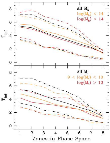
Figure 6: Solid lines trace the mean infall time, $\overline{\rm T}$_inf, in Gyr as a function of zone in projected phase-space and in different bins of halo mass (top panel) and stellar mass (bottom panel) as derived from the YZiCS hydrodynamic simulations. The 25^th and 75^th percentiles of the T_inf distribution within each zone are plotted with dashed lines. The simulated dwarf galaxies are not shown in this figure because the log(M${}_{\star})<$ 9 bin is not included in the analysis of our data; for each zone, their $\overline{\rm T}$_inf is slightly longer than that of the ‘All M_⋆’ sample.

Table 2 summarizes the main properties of the YZiCS simulation set in each zone in projected phase-space, including $\overline{\rm T}$_inf in Gyr, and its associated standard deviation $\sigma$($\overline{\rm T}$_inf), as well as the average fraction of dark matter subhalo stripped from satellites $<$ f${}_{\rm dm}>$ and its standard deviation $\sigma$($<$ f${}_{\rm dm}>$). We also report in the table the fraction of interlopers f_intl and the fraction of satellites (interlopers excluded) that have not yet had a pericentric passage f_no-per. In Appendix A we discuss in detail how much projection effects result in cross-contaminations of the zones in terms of T_inf.

As these results are derived from one set of cosmological simulations, it is likely that we can expect some changes in $\overline{\rm T}$_inf and shape of the T_inf distribution in each zone if using a different set of simulations. These differences could arise from having different sample size, differing cosmological parameters, or more technical issues such as different mass and spatial resolution, or differing definitions of haloes and their boundaries. Nevertheless, we are confident that the mean T_inf will always systematically decrease with increasing zone number. Indeed we have confirmed that this is the case in the Millennium simulations. This fact is key to our methodology and the main conclusions of this study as it enables us to see how the galaxy population properties change when we alter the population’s average T_inf.

4 Satellite observed properties in projected phase-space

Numerical and hydro-dynamical simulations of environmental effects such as ram-pressure and tidal stripping show that satellites are deprived of their gas and stars outside-in, and the amplitude of this removal should depend on their stellar mass, their orbit within their host halo, the dark-matter mass of the host, and the time when they were accreted onto their host environment. As a consequence, we expect to detect a dependence of the observed properties of satellites in their projected phase-space since this is simply a parameterization of their orbits and hence infall histories.

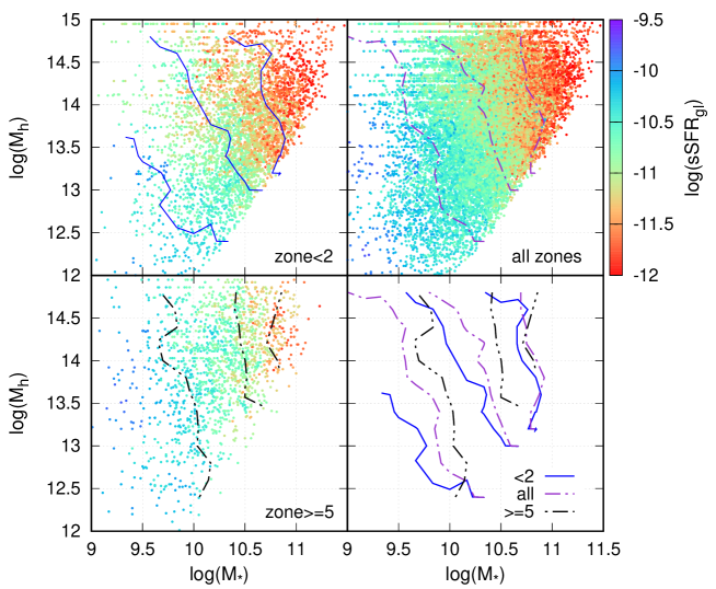
Figure 7: Galaxy specific star formation rate as a function of galaxy M_⋆ and host M_h for our working sample. Contours are shown at log(sSFR_gl) = -10.5, -11.0, -11.5 (from left to right). The upper-right panel shows the full sample. The upper-left panel shows galaxies in zone $\leq$ 2 ($\overline{\rm T}$${}_{\rm inf}\geq$ 5 Gyr). The lower-left panel shows galaxies in zone $\geq$ 5 ($\overline{\rm T}$${}_{\rm inf}\leq$ 3.4 Gyr). The lower-right panel shows how the contour shape and position change when $\overline{\rm T}$_inf shifted.

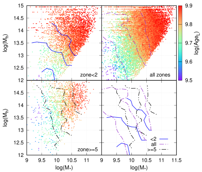
Figure 8: As in Fig. 6 but for luminosity-weighted age instead of specific star formation rate. Contours are shown at log(Age_L) = 9.7, 9.8, 9.85 (from left to right). Galaxies in zone $\leq$ 2 have $\overline{\rm T}$${}_{\rm inf}\geq$ 5 Gyr, while those in zone $\geq$ 5 have $\overline{\rm T}$${}_{\rm inf}\leq$ 3.4 Gyr.

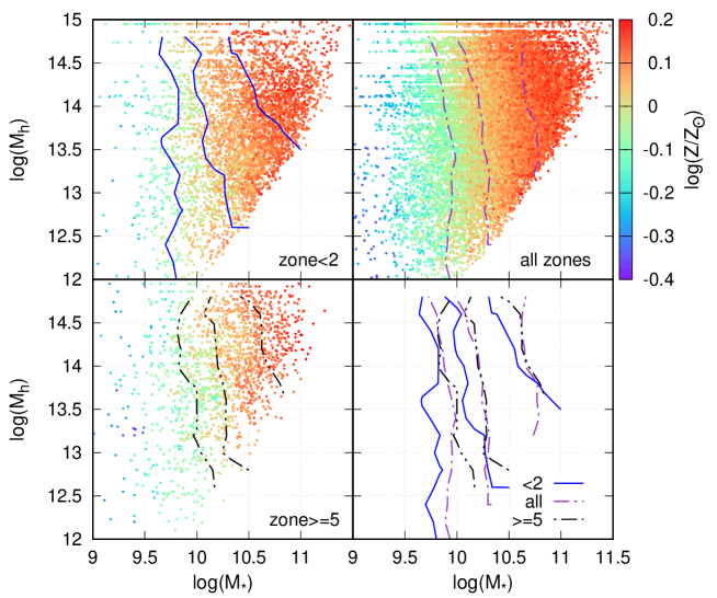
Figure 9: As in Fig. 6 but for stellar metallicity instead of specific star formation rate. Contours are shown at log(Z/Z_⊙) = -0.025, 0.05, 0.125 (from left to right). Galaxies in zone $\leq$ 2 have $\overline{\rm T}$${}_{\rm inf}\geq$ 5 Gyr, while those in zone $\geq$ 5 have $\overline{\rm T}$${}_{\rm inf}\leq$ 3.4 Gyr.

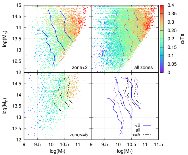
Figure 10: As in Fig. 6 but for [$\alpha$/Fe] element ratio instead of specific star formation rate. Contours are shown at [$\alpha$/Fe] = 0.2, 0.24, 0.275 (from left to right). Galaxies in zone $\leq$ 2 have $\overline{\rm T}$${}_{\rm inf}\geq$ 5 Gyr, while those in zone $\geq$ 5 have $\overline{\rm T}$${}_{\rm inf}\leq$ 3.4 Gyr.

4.1 Observed global distributions

We use the $|\Delta V|$/$\sigma$ and R_proj/R₂₀₀ values measured for our working sample and Eq.(3) and (4) to assign each satellite a zone in projected phase-space and thus a $\overline{\rm T}$_inf value. We then plot each galaxy’s location in the log(M_⋆) and log(M_h) plane, and colour the point by galaxy property. In this way, we can effectively see how galaxy properties vary as we simultaneously control for the effect of galaxy mass and host mass (which is our proxy for environment). In order to look for large scale trends across the plot, we plot for each galaxy the average property of its nearest 30 neighbours in the log(M_⋆) - log(M_h) plane. This average also takes into account the weighing required to correct for our observational biases (discussed in Sect. 2). The results are shown in Figs. 7 to 10. In each plot we consider a different galaxy property, and in each panel we split the sample by zone. Satellites with zone $<$ 2 (corresponding to $\overline{\rm T}$${}_{\rm inf}\geq$ 5 Gyr) and zone $\geq$ 5 (with $\overline{\rm T}$${}_{\rm inf}\leq$ 3.4 Gyr) are shown in the top left and bottom left panels, respectively, and all zones combined are shown in the top right panel.

We overlay contours at three fixed values on each distribution, and compare them in the bottom right panel of Figs. 7 - 10. To make the contours, we first bin up the log(M_h)-log(M_⋆) plane presented in the Figures into a 15 $\times$ 15 pixels grid, and compute the mean value in each pixel. Contours are then fitted to the gridded values.

A visual inspection of the all-zone distributions clearly shows that, at fixed M_h, satellites become more passive and older, as well as metal-richer and enriched in $\alpha$-elements, with increasing M_⋆. A weaker trend in host halo mass is detectable for sSFR_gl and Age_L at fixed M_⋆ (cf. Pasquali et al. 2010), which disappears in the distributions of recent infallers, i.e. satellites with zone $\geq$ 5. The picture though changes for the ancient infallers in zone $<$ 2, since their sSFR_gl, Age_L and possibly [$\alpha$/Fe] appear to depend on M_⋆ and more clearly on halo mass. In fact, at fixed M_⋆, sample satellites grow more passive and older with increasing M_h (this dependence is weaker for [$\alpha$/Fe]). These changes already start to occur at the lower host masses, a feature that does not emerge in the all-zone distributions: we first need to control for the effect of infall time in order to clearly bring out the effects of lower mass hosts.

At the same time, we see that the contours progressively move to lower stellar and halo masses as we shift zone from 5 to 2, and hence increase $\overline{\rm T}$_inf at fixed contour level. This is clearly seen for sSFR_gl and Age_L, and, at lower extent, for stellar metallicity and [$\alpha$/Fe]. We also note how, at fixed contour level, these contours become less steep and bend over with increasing $\overline{\rm T}$_inf, particularly in the case of sSFR_gl and Age_L.

These results indicate that sSFR_gl and Age_L of a satellite primarily depend on its stellar mass when such satellite is a recent infaller, while it additionally depends on M_h when the satellite was accreted at earlier times, i.e. when environmental effects have been at play for a longer time. Moreover, the dependence of sSFR_gl and Age_L of ancient infallers on M_h indicates that, upon infall, the environment takes several Gyrs to quench satellites, and more massive haloes are more efficient in extinguishing the star formation activity of satellites. In the case of stellar metallicity and [$\alpha$/Fe], the separation of our sample satellites into different zones (or differing $\overline{\rm T}$_inf) does not highlight any significant trend of log(Z/Z_⊙) with M_h at fixed M_⋆. In other words, the galaxies seem to obey the mass-metallicity relation, nearly independent of their environment.

One caveat is that, in Figure 6, we can see that more massive satellites (log(M_⋆ M${}_{\odot}h^{-2})>$ 10) have slightly reduced $\overline{\rm T}$_inf values than less massive satellites (9 $<$ log(M_⋆ M${}_{\odot}h^{-2})<$ 10), in particular at the zone 1 end, although the difference is small ($<$0.75 Gyr) and well within the scatter in the trend. For Figs. 7 to 11, this implies there is a small decrease in $\overline{\rm T}$_inf along the log(M_⋆) axis, affecting the zone $<$ 2 panels only. This small decrease in $\overline{\rm T}$_inf might slightly reduce environmental quenching, and thus the effect might be to fractionally counteract the mass quenching trend in the zone $<$ 2 panels only.

4.2 Trends of satellite observed properties with zone

We now turn to investigate in more detail the dependence of the satellite properties on zone in projected phase-space, using a more quantified and less visual approach than previously. For this purpose, we split the satellites of our working sample in 2D bins defined by stellar mass and halo mass as follows:

• 9 $\leq$ log(M_⋆ M${}_{\odot}h^{-2})<$ 10, since Pasquali et al. (2010) showed that satellites in this stellar mass range are most sensitive to environmental effects;

• 10 $\leq$ log(M_⋆ M${}_{\odot}h^{-2})<$ 10.5, which we consider a transition range, representing galaxies which are less affected by environmental processes;

• 10.5 $\leq$ log(M_⋆ M${}_{\odot}h^{-2})\leq$ 11.5, since Pasquali et al. (2010) found that the stellar properties of such massive satellites are the least environmentally dependent;

and:

• 12 $\leq$ log(M_h M${}_{\odot}h^{-1})<$ 13, the low mass environments;

• 13 $\leq$ log(M_h M${}_{\odot}h^{-1})<$ 14, the intermediate mass host haloes;

• 14 $\leq$ log(M_h M${}_{\odot}h^{-1})\leq$ 15, the massive environments.

This stacking is meant not only to provide sufficient statistics for our analysis, but also to reduce the noise due to errors on the observed line-of-sight velocity and cluster-centric distance of the satellites in our working sample. The galaxy statistics available for these 2D bins is summarized in Table 3. For each 2D mass bin, we derive the average of a specific galaxy property weighted by (1/V${}_{\rm max}\times w_{SN}$) from all satellites belonging to the same zone in phase-space, and also compute the standard error on the weighted mean. We consider only those zones which contain at least 20 satellites each.

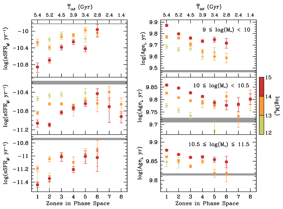
Figure 11: The observed distribution of average global sSFR and average age of our sample satellites as a function of zone and $\overline{\rm T}$_inf in projected phase-space in the left-hand and right-hand column respectively. The error bars represent the error on the mean. Satellites are split into three bins of stellar mass (from 10⁹ to 10^11.5 M${}_{\sun}h^{-2}$) and 3 bins of halo mass: 12 $\leq$ log[M_h (M${}_{\sun}h^{-1}$)] $<$ 13 (yellow triangles), 13 $\leq$ log[M_h (M${}_{\sun}h^{-1}$)] $<$ 14 (orange squares) and 14 $\leq$ log[M_h (M${}_{\sun}h^{-1}$)] $\leq$ 15 (red circles). Each grey shaded area represents the range in weighted mean sSFR_gl and Age_L spanned by field galaxies.

Table 3: The number of satellites in our working sample per bin of log(M_⋆ M${}_{\odot}h^{-2}$) and log(M_h M${}_{\odot}h^{-1}$).

			log(Mh)
log(M⋆)		12 - 13	13 - 14	14 - 15
9.0 - 10.0		775	1267	1257
10.0 - 10.5		921	4468	3377
10.5 - 11.5		74	4176	4428

4.2.1 Specific SFR as a function of $\overline{\rm T}$_inf

In the left-hand column of Fig. 11 we plot the average global sSFR as a function of zone and $\overline{\rm T}$_inf for satellites separated into the three M_⋆ bins and colour-coded on the basis of the three M_h bins defined above. Each grey shaded area shows the range in weighted mean sSFR_gl spanned by field galaxies in each M_⋆ bin (see Sect. 4.3). A trend of increasing log(sSFR_gl) with increasing zone number, hence decreasing $\overline{\rm T}$_inf, is visible between zones 1 to 6, which is stronger for satellites in more massive haloes (red circles). We estimate by how much sSFR_gl varies between zones 1 and 6, and see that this variation $\Delta$ increases with halo mass. At log(M_⋆ M${}_{\odot}h^{-2})\leq$ 10.5, $\Delta$ is $\sim$0.15, $\sim$0.25 and $\sim$0.65 dex in low-, intermediate- and high-mass hosts, respectively. For the more massive satellites, $\Delta$ is $\sim$0.3 and 0.4 dex in intermediate- and high-mass haloes, respectively. An interesting feature of the intermediate-mass satellites in $>$10¹³ M${}_{\odot}h^{-1}$ haloes is the flattening of their distribution to lower sSFR_gl values at zone $>$ 6.

We also notice that, for satellites less massive than log(M_⋆ M${}_{\sun}h^{-2}$) = 10.5 and in zones $<$ 4, the average sSFR_gl is generally higher in low-mass haloes, and decreases with increasing M_h. In other words, at fixed stellar mass and fixed zone (for the same $\overline{\rm T}$_inf), the quenching of the star-formation activity of satellites is controlled by the halo mass of the host, and is more efficient in more massive hosts.

The above trends are qualitatively consistent with the results of Hernández-Fernández et al. (2014) who found that colour-selected passive galaxies in 16 clusters at $z<$ 0.05 are preferentially distributed in phase-space within the caustic profile ($|\Delta{\rm V}|/\sigma_{\rm los})$ $\times$ (R_p/R${}_{\rm 200})\sol$ 0.4 (corresponding to our zones $\sol$ 3 in Fig. 4), while the distribution of star-forming galaxies extends to higher caustic profiles (or higher zone numbers). Similarly to our results for $z\sim$ 0 galaxy groups and clusters, Noble at al. (2013) and Noble et al. (2016) observed a remarkable increase ($\sim$1 - 2 dex) in sSFR with increasing values of ($|\Delta{\rm V}|/\sigma_{\rm los})$ $\times$ (R_p/R₂₀₀), hence with increasing zone number, in a cluster at $z$ = 0.87 and in three clusters at $z$ = 1.2. More recently, Barsanti et al. (2018) found that the fraction of star-forming galaxies in the Galaxy And Mass Assembly (GAMA) group catalogue (at 0.05 $\leq z\leq$ 0.2) is higher in the outer region of their projected phase-space (corresponding to higher zone numbers).

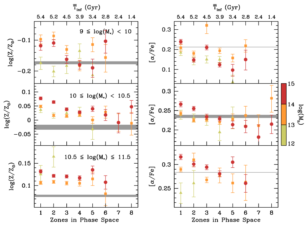
Figure 12: As in Fig. 11 but now for average stellar metallicity and average [$\alpha$/Fe] ratio of satellites in our working sample. Each grey shaded area represents the range in weighted mean log(Z/Z_⊙) and [$\alpha$/Fe] spanned by field galaxies.

4.2.2 Stellar age as a function of $\overline{\rm T}$_inf

The right-hand column of Fig. 11 shows the average, luminosity-weighted stellar age of satellites as a function of zone and $\overline{\rm T}$_inf for the same M_⋆ and M_h bins as in the left-hand column. Also in this case the grey stripes show the ranges in Age_L covered by field galaxies.

The behaviour of stellar age is opposite to that of average sSFR_gl, as it clearly decreases with increasing zone number (thus with decreasing $\overline{\rm T}$_inf), at least up to zone 6. The amplitude $\Delta$ of the age variation between zone 1 and 6 is larger for low mass satellites (M${}_{\star}<$ 10¹⁰ M${}_{\sun}h^{-2}$), and it increases from $\sim$0.7 Gyr in low-mass host haloes (yellow triangles) to $\sim$2 Gyr in host haloes more massive than log(M_h M${}_{\sun}h^{-1}$) = 13 (orange squares and red circles). For intermediate-mass satellites $\Delta$ is $\sim$1 Gyr, while it decreases to $\sim$0.6 Gyr at M${}_{\star}>$ 10^10.5 M${}_{\sun}h^{-2}$. As in the case of sSFR_gl, we point to the flattening of the age distribution of intermediate-mass satellites in host haloes more massive than 10¹³ M${}_{\sun}h^{-1}$ at zone $>$ 6.

We also observe that, at fixed stellar mass and zone (for zone $<$ 6), satellites become progressively older as the halo mass of their host groups increases, which adds further support for the M_h-driven quenching of galaxy star formation. At fixed host halo mass the mean stellar age of satellites can be seen to increase with stellar mass (see also Pasquali et al. 2010).

The above results are qualitatively similar to the analysis performed by Noble et al. (2013) and Noble et al. (2016), who traced the dependence of the age indicator D4000 on caustic profiles for galaxies in clusters at $z$ = 0.87 and 1.2. They showed that D4000 steadily decreases with increasing ($|\Delta{\rm V}|/\sigma_{\rm los})$ $\times$ (R_p/R${}_{\rm 200})$ (hence with increasing zone number), so that galaxies exhibit progressively younger ages for larger values of caustic profile.

4.2.3 Stellar metallicity as a function of $\overline{\rm T}$_inf

We plot the average stellar metallicity as a function of zone and $\overline{\rm T}$_inf, and per bin of stellar and halo mass in the left-hand column of Fig. 12 (the grey shaded areas represent the range in weighted mean log(Z/Z_⊙) of field galaxies). Despite the noise in the distributions, a weak trend of decreasing metallicity with increasing zone number (hence decreasing $\overline{\rm T}$_inf) can be recognised at stellar masses log(M_⋆ M${}_{\sun}h^{-2}$) $\leq$ 10.5 and log(M_h M${}_{\sun}h^{-1}$) $\geq$ 13. Its amplitude between zones 1 and 6 is $\Delta\sim$ 0.05 dex for low mass satellites, and $\Delta\sim$ 0.04 dex for intermediate-mass satellites. The average stellar metallicity of more massive satellites is essentially invariant with zone. The Z distribution of intermediate-mass satellites in massive haloes shows a flattening at zone $>$ 6, where stellar metallicity levels off within the error bars.

In the case of satellites more massive than M_⋆ = 10¹⁰ M${}_{\sun}h^{-2}$ and for zone $<$ 5 the average log(Z/Z_⊙) slightly increases with M_h at fixed stellar mass and zone (similarly to that found by Pasquali et al. 2010, although less pronounced). We also notice that, at fixed halo mass, the average log(Z/Z_⊙) increases with stellar mass as expected from the known galaxy metallicity - mass relation (e.g. Tremonti et al. 2004, Gallazzi et al. 2005, Mannucci et al. 2010, Foster et al. 2012, Sánchez et al. 2017).

4.2.4 [$\alpha$/Fe] ratio as a function of $\overline{\rm T}$_inf

The [$\alpha$/Fe] element ratio is shown as a function of zone and $\overline{\rm T}$_inf in the right-hand column of Fig. 12 for satellite and field galaxies. First of all, we notice that, regardless of zone, at fixed halo mass, [$\alpha$/Fe] increases with stellar mass, but no systematic dependence of [$\alpha$/Fe] on halo mass at fixed M_⋆ can be found. This reproduces the findings of Gallazzi et al. (2018, in prep) that the relation between [$\alpha$/Fe] and M_⋆ is to first order independent of halo mass. Here, by studying the distribution of [$\alpha$/Fe] in projected phase-space we can identify a trend of decreasing [$\alpha$/Fe] with increasing zone number (decreasing $\overline{\rm T}$_inf) in particular for satellites in haloes more massive than 10¹⁴ M${}_{\odot}h^{-1}$. For this halo mass range, the amplitude $\Delta$ of the overall change in [$\alpha$/Fe] between zones 1 and zones 6 depends on M_⋆: it varies from $\sim$0.1 dex at low stellar masses to $\sim$0.05 dex for intermediate and high masses.

We have checked that the above trends do not significantly depend on our weighing scheme. In the extreme case when galaxy properties are weighted only by 1/V_max, the trends in Figs. 11 and 12 are seen to shift to older ages, higher metallicity and [$\alpha$/Fe] values, and to lower sSFR_gl values by an amount typically less than 3$\sigma$, while their gradients become less steep. In order to check the effect of the uncertainty on the group centre definition, we have computed mean galaxy properties as a function of zone using the projected distance of satellites from their central galaxy, and weighing galaxy properties by (1/V${}_{\rm max}\times w_{SN}$). The new trends are largely consistent with those shown in Figs. 11 and 12. We have also calculated how the mean observed galaxy properties change as a function of the caustic regions defined in Sect. 3.1, where $|\Delta V|$/$\sigma$ $\times$ R_proj/R₂₀₀ varies from 0.1 to 1.0 in steps of 0.1. We find trends similar to those obtained with our zones approach, albeit more noisy.

4.3 Comparison with the field

It is interesting to check how the trends of the observed properties of satellites in projected phase-space compare with the average properties of field galaxies.

We use the DR7 group catalogue of Wang et al. (2014) to define the field population using three different criteria: (i) by extracting all central galaxies residing in haloes less massive than M_h = 10¹² M${}_{\sun}h^{-1}$; (ii) by retrieving all centrals with no associated satellite (down to the magnitude limit of the SDSS spectroscopy); (iii) by selecting all galaxies of (ii) which are more than 5R₂₀₀ away from their closest environment which is not their host halo. In all cases, we keep only those galaxies whose spectral S/N is 20 or higher. We notice that criteria (i) provides us with centrals less massive than M_⋆ = 10^10.5 M${}_{\sun}h^{-2}$, while the centrals chosen by criteria (ii) and (iii) populate the whole stellar mass range of the satellites in our working sample.

For each sample, we compute the weighted average sSFR_gl, Age_L, log(Z/Z_⊙) and [$\alpha$/Fe] in each stellar mass bin. We then plot the range defined by the mean galaxy properties of the three samples as a grey shaded area in Figs. 11 and 12.

Field galaxies are more strongly star forming and have younger luminosity-weighted ages at any M_⋆ than equally massive satellites, although in some cases satellites in zone $\geq$ 6 are consistent with the field population at the 1 - 2$\sigma$ level. The average age of low mass satellites exhibits the strongest deviation from the field, indicating once again that they are the galaxies most prone to environmental effects.

We observe a clear offset in log(Z/Z_⊙) between the field population and satellites more massive than log(M_⋆ M${}_{\sun}h^{-2}$) = 10, in that satellites in zone $<$ 6 are metal-richer by $\sim$0.05 dex. Satellites with higher zone number have a stellar metallicity more similar to that of field galaxies. In the case of low mass satellites, we see a trend with halo mass: those residing in low mass haloes are as metal-rich as field galaxies at the 1$\sigma$ level, while satellites living in intermediate- and high mass haloes are $\sim$0.06 dex metal-richer than the field if in zone $<$ 3, else have log(Z/Z_⊙) similar to that of field galaxies at the 1 - 2$\sigma$ level.

Finally, only satellites with log(M_⋆ M${}_{\odot}h^{-2})>$ 10, log(M_h M${}_{\odot}h^{-1})>$ 14 and zone $<$ 3 show a [$\alpha$/Fe] abundance ratio slightly higher than the field, while they become comparable with the field population at zone $>$ 3 similarly to equally massive satellites in lower mass haloes at any zone. Low mass satellites in low- and high mass environments display [$\alpha$/Fe] values lower than the field.

In conclusion, we see satellite properties generally approaching the field values with increasing zone number, and nearly equalling the field for low mass hosts. On the contrary, the average observed properties of satellites in more massive environments often seem to flatten out before reaching the field values.

5 Discussion

Dissecting the projected phase-space of galaxy groups/clusters into zones of constant mean infall time has allowed us to emphasize the dependence of galaxy properties on environment while controlling for the effects of both galaxy and halo mass. In what follows we will discuss the environmental processes responsible for the observed trends in projected phase-space, we will also use the observed dependence of galaxy properties on $\overline{\rm T}$_inf to estimate time-scales for the quenching of star formation, and to address satellite pre-processing. We will refer to satellites in low number zones as ’ancient infallers’, and to satellites in high number zones as ’recent infallers’.

5.1 Nurture at work

The information on zones in projected phase-space has allowed us to bring out the dependence of sSFR_gl and Age_L of ancient infallers on halo mass (cf. Figs. 7 and 8, also Barsanti et al. 2018), which would otherwise go undetected when mixing satellites of different T_inf (see Peng et al. 2010). More specifically, at fixed M_⋆ the satellites’ sSFR_gl smoothly increases with zone while their Age_L decreases, indicating that ancient infallers are more quenched than recent infallers. In addition, at fixed zone, satellites’ sSFR_gl and Age_L tend to decrease and increase, respectively, with increasing halo mass (cf. Fig. 11). We interpret these trends as the result of the early T_inf of ancient infallers, which thus underwent gas loss via strangulation and ram-pressure stripping at earlier times and for longer durations. The strength of these environmental effects is obviously amplified in more massive host haloes because of their deeper potential well and denser intracluster medium, both of which make gas removal and star-formation quenching more efficient.

The trends in the distribution of metallicity as a function of zone are far less pronounced than those in sSFR_gl and Age_L. However, a general increase of Z with decreasing zone can be recognized for satellites less massive than log(M_⋆ M${}_{\odot}h^{-2})=$ 10.5 and residing in more massive haloes. These results are likely the effect of ram-pressure stripping with some possible contribution from tidal stripping. As ram-pressure stripping proceeds outside-in, it removes the satellite outskirts that are typically metal-poor, and inhibits radial gas inflows which otherwise would dilute the gas-phase metallicity in the central region of the satellite (see also Pasquali et al. 2012). Bahé et al. (2017) showed that the absence of metal-poor gas inflows allows a satellite to form stars from metal-rich gas and hence to increase its overall stellar metallicity by an amount which seems to be consistent with the metallicity difference between satellites and the field population in Fig. 12. The longer exposure to ram pressure stripping can thus justify the higher metal content of ancient infallers with respect to recent ones.

This scenario is somehow corroborated by the fact that satellites have similar [$\alpha$/Fe] as the field population, indicating a similar duration of their star formation activity although it occurs at lower sSFR_gl in satellites. Therefore, the higher metal content of satellites with respect to the field is not due to stronger or more efficient star formation in satellites, but possibly to star formation taking place in metal-richer gas. We note here that the weak trend of increasing [$\alpha$/Fe] with $\overline{\rm T}$_inf possibly indicates an early truncation of star formation in ancient infallers, when [$\alpha$/Fe] is used as a proxy for the duration of the star formation activity in galaxies (cf. de La Rosa et al. 2011). Nevertheless, the galaxy formation models of De Lucia et al. (2017) have highlighted that [$\alpha$/Fe] may not be a straightforward indicator of the time-scale of star formation as it significantly depends on the intensity of star formation and on other galaxy properties such as AGN feedback (cf. Segers et al. 2016), galactic winds and the Initial Mass Function (cf. Fontanot et al. 2017).

The trend of increasing log(Z/Z_⊙) with $\overline{\rm T}$_inf could also be due to tidal stripping. If a galaxy initially sits on the normal stellar mass-metallicity relation, then after losing stellar mass it may appear too metal-rich for its new stellar mass, compared to typical galaxies (see also Pasquali et al. 2010). Increasing the time spent in a host might result in a larger stellar mass loss, which would thus explain the trend of rising stellar metallicity with increasing $\overline{\rm T}$_inf. In the following, we attempt to roughly estimate how much stellar mass would need to be stripped to explain the average metallicity of zone 1 satellites. First, we define the relation between stellar mass and metallicity followed by all centrals which have a spectral S/N $\geq$ 20 in the Gallazzi et al.’s (2018 in prep) catologue, by calculating the weighted average metallicity in small bins of stellar mass. We then use this relation to read the stellar mass corresponding to the average metallicity of zone 1 satellites, and we dub the difference between this value and the mean M_⋆ of zone 1 satellites as stellar mass loss. We find that such stellar mass loss is typically 0.25 dex, quite independently of the stellar and halo mass as also found by Han et al. (2018) using the same YZiCS simulations. On average, 80$\%$ stellar mass loss would be necessary to explain the metallicity of ancient infallers through tidal stripping of their progenitor.

This value is somehow higher than the fraction of stripped dark matter (f_dm in Table 2) in zone 1, and, together with the fact that dark-matter haloes are more easy to strip, suggests that stellar mass loss alone is unlikely to fully explain our result of increasing log(Z/Z_⊙) with $\overline{\rm T}$_inf. A fraction of the satellites in zone 1 may have suffered enough tidal mass loss to reach these metallicities, but they are not enough to match the mean observed metallicity.

Table 4: The mean pericentric distance ($<$R_per/R${}_{\rm vir}>$) and orbit eccentricity ($<e>$), computed in projected phase-space from the simulations of Warnick & Knebe (2006), as a function of zone and mean infall time $\overline{\rm T}$_inf (in Gyr).

Zone	$\overline{\rm T}$inf	$<$Rper/R${}_{\rm vir}>$	$\sigma$($<$Rper/R${}_{\rm vir}>$)	$<e>$	$\sigma$($<e>$)
1	5.42	0.220	0.233	0.552	0.221
2	5.18	0.296	0.280	0.559	0.232
3	4.50	0.355	0.319	0.574	0.243
4	3.89	0.436	0.392	0.585	0.253
5	3.36	0.516	0.429	0.557	0.266
6	2.77	0.547	0.403	0.552	0.277
7	2.24	0.581	0.414	0.555	0.281
8	1.42	0.588	0.437	0.562	0.286

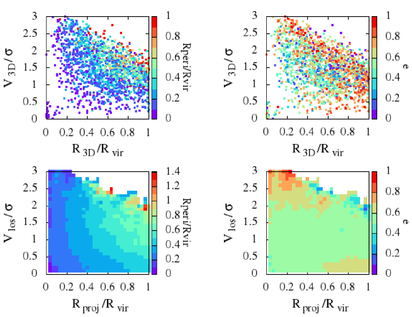
Figure 13: Top panels: the distributions of pericentric distance in units of virial radius, R_peri/R_vir, and orbit eccentricity, $e$, across the 3D phase-space diagram in Warnick & Knebe’s (2006) simulations. Bottom panels: the distributions of R_peri/R_vir and $e$ on the 2D, projected phase-space diagram in Warnick & Knebe’s (2006) simulations.

5.1.1 The effect of orbital parameters

Ram-pressure and tidal stripping not only depend on the dark matter density distribution of a halo, or the density of its intracluster medium, but also on the orbital velocity of a galaxy in that halo. All of these should vary with location along the orbit, and the variation might be expected to be larger for objects on more eccentric orbits. Figure 1 of Rhee et al. (2017) presents a toy representation of a typical trajectory that an infalling galaxy takes on a 3D phase-space diagram. Although both orbital velocity and cluster-centric radius fluctuate with time, overall objects tend to shift toward lower orbital velocity and cluster-centric distance as time passes by (see also the left panel of Figure 2 of Rhee et al. 2017). This change is partly the result of dynamical friction, which steadily dissipates the orbital energy of satellites, especially for massive galaxies. In addition, all satellites are influenced by the deepening and changing shape of the potential well in which they orbit as their hosts haloes grow in mass by accretion. This effect is also thought to be responsible for satellite orbits becoming increasingly circularised with time (Gill et al. 2004). The net result of these effects is that, with increasing T_inf, satellites are found closer to the central region of their host halo, where the intracluster medium is denser and the halo potential well is deeper. If their orbits become more circularised, they will spend longer periods of time near the centre, and may become increasingly quenched and tidally stripped (of gas and stars). It is thus interesting to use the simulations to compute the mean orbital parameters, pericentric distance and orbit eccentricity, as a function of zone and $\overline{\rm T}$_inf (see Table 4), and compare them with the trends of observed galaxy properties in projected phase-space.

In the top panels of Fig. 13 we plot the satellites simulated by Warnick & Knebe (2006) in a 3D phase-space diagram. The data points are colour coded on the basis of their normalised pericentre distance R_peri/R_vir (left-hand panel), and their orbital eccentricity $e$ (right-hand panel). In a 3D phase-space diagram, it is clear that both pericentre distance and eccentricity vary accross the diagrams. For example, we see that the pericentric distance increases with cluster-centric distance and also with orbital velocity. The distribution is somewhat similar to the distribution of T_inf in projected phase-space, as shown in Fig. 4. The orbital eccentricity distribution is a little more complex with high values of eccentricity found at both high and low velocities simultaneously. Objects with a combination of both small pericentric distances and small orbit eccentricities (i.e. rounder orbits) tend to be located in more central regions of the 3D phase-space diagram.

In the bottom panels of Fig. 13, we present projected phase-space diagrams. For these we consider 100 randomly chosen line-of-sights, and build up the mean normalised pericentre distance (lower-left panel) and orbital eccentricity distribution (lower-right panel) in each pixel. The projected distribution of pericentre distance has a similar trend to the 3D version, only it appears more smoothed. However, projection effects wash out most of the trend seen in the 3D orbital eccentricity plot. These results are also confirmed quantitatively by the mean values of R_peri/R_vir and $e$ shown in Table 4, which we computed for each zone, together with their standard deviation. Ancient infallers are, on average, characterized by small pericentric distances (R_peri/R_vir $\simeq$ 0.2 - 0.3), while recent infallers have R_peri/R_vir $\sim$ 0.6. We conclude that the large T_inf of ancient infallers has resulted in a population of galaxies with small pericentric distance and lowered eccentricity, thus making these satellites spend more time in the central region of their host haloes. This could partly contribute to the fact that we see the strongest environmental effects in this population, as these galaxies will spend most of the time near their host’s centre where environmental effects are likely most effective. However, if the impact of some environmental mechanisms is accumulated with time, then environmental effects would be most visible in the population of galaxies that have spent most time in the cluster, and thus the change in orbital parameters may only provide an additional contribution to the overall change. We also note that, although we can confirm that orbital circularisation can be seen to occur in our 3D phase space diagram, a lot of the eccentricy variation is washed out in the projected phase space diagrams, and as a result it may be difficult to detect orbital circularisation in observed phase space diagrams.

5.2 Further implications of the observed trends in project phase-space

5.2.1 Quenching time-scales

Table 5: The gradient and intercept of the linear fits of observed sSFR_gl vs. $\overline{\rm T}$_inf, together with the estimated quenching time-scale $\Delta t_{\rm q}$ and their corresponding errors.

log(M⋆ M${}_{\odot}h^{-2}$)	Parameters	Units		log(Mh M${}_{\odot}h^{-1}$)
			12 - 13	13 - 14	14 - 15
9.0 - 10.0	$\frac{\Delta(\rm{sSFR_{\rm gl}})}{\Delta t}$	10-11yr-1Gyr-1	-2.398 $\pm$ 0.185	-2.370 $\pm$ 0.159	-3.197 $\pm$ 0.229
	Intercept	10-11yr-1	15.834 $\pm$ 0.249	15.854 $\pm$ 0.226	15.863 $\pm$ 0.251
	$\Delta t_{\rm q}$	Gyr	6.187 $\pm$ 0.488	6.268 $\pm$ 0.432	4.649 $\pm$ 0.342
10.0 - 10.5	$\frac{\Delta(\rm{sSFR_{\rm gl}})}{\Delta t}$	10-11yr-1Gyr-1	-0.861 $\pm$ 0.189	-1.151 $\pm$ 0.114	-1.273 $\pm$ 0.047
	Intercept	10-11yr-1	6.232 $\pm$ 0.509	6.211 $\pm$ 0.268	6.327 $\pm$ 0.106
	$\Delta t_{\rm q}$	Gyr	6.075 $\pm$ 1.456	4.528 $\pm$ 0.504	4.183 $\pm$ 0.176
10.5 - 11.5	$\frac{\Delta(\rm{sSFR_{\rm gl}})}{\Delta t}$	10-11yr-1Gyr-1	-0.309 $\pm$ 0.009	-0.223 $\pm$ 0.054	-0.283 $\pm$ 0.067
	Intercept	10-11yr-1	1.734 $\pm$ 0.033	1.724 $\pm$ 0.191	1.723 $\pm$ 0.225
	$\Delta t_{\rm q}$	Gyr	2.375 $\pm$ 0.129	3.243 $\pm$ 1.164	2.551 $\pm$ 0.997

As the phase-space analysis provides us with constraints on the average time that galaxies have spent in their hosts, we can now examine how their observed mean sSFR_gl changes as a function of time in their host, for hosts and satellites of different mass. To do so, we consider zones 1 to 6, and associate them with their $\overline{\rm T}$_inf as listed in Table 2. We can also use the field sSFR_gl value as our $\overline{\rm T}$${}_{\rm inf}=$ 0 data point. This is the mean among the field sSFR_gl values derived with methods $(i)$, $(ii)$ and $(iii)$ described in Sect.4.3, and its associated error is half the full sSFR_gl range computed for field galaxies at fixed stellar mass. In general, we find that the time evolution of the observed decline in mean sSFR_gl has a very linear form. Only in zones 7 and 8 of the intermediate mass satellites do we find some deviation from the linear fit, where some reduced values of sSFR_gl are found (probably due to pre-processing as discussed below), and so we neglect these data points when conducting the linear fit. We then perform a simple linear fit of observed mean sSFR_gl vs. $\overline{\rm T}$_inf, which takes into account the errors on sSFR_gl (as shown in Fig. 11) and the standard deviation on $\overline{\rm T}$_inf (as listed in Table 2). The resulting best-fit gradient, intercept and associated errors are reported in Table 5 together with their units.

In general, comparing between columns in the table, we can see that the rate of reduction of the mean sSFR_gl after entering a host is higher for more massive hosts, possibly because of their denser intracluster medium. This trend is though not visible in our highest stellar mass bin, thus suggesting that internal mass quenching is more dominant for these galaxies, which, in addition, tend to be accreted later. In any case, even for the massive satellites, their sSFR_gl continues to decline with time spent in their host, albeit at a slower rate than for less massive galaxies. Comparing between stellar masses (i.e. comparing rows in the table), we see that the rate of decline of the mean sSFR_gl is much higher for low mass satellites than high mass satellites. This further supports the fact that low mass satellites are more sensitive to environment. We caution here that the analysis above is qualitatively correct as far as we can associate satellites with field galaxies of the same present-day stellar mass as their progenitors.

In the literature, the star-formation quenching time-scale is often defined as the time needed for a satellite’s sSFR to fall below a critical value of 10^-11 yr^-1 after infalling into its host. Thus, we repeat this approach using our linear fits, and calculate the time it takes to reach this critical value, which we dub $\Delta t_{\rm q}$ (in Gyr) in Table 5. We can see that, similar to the rate of decline of sSFR_gl, at fixed stellar mass $\Delta t_{\rm q}$ becomes shorter in more massive environments, once again with the unique exception of the most massive stellar mass bin. Now considering fixed halo mass, $\Delta t_{\rm q}$ becomes instead shorter for more massive satellite. This is the opposite to what we found for the rate of decline of the sSFR_gl which happens more slowly in massive satellites. This is, once again, a result of the fact that the high mass satellites have low sSFR_gl values even prior to infall into their host. For example, in the table we can see that satellites in the highest stellar mass bin have a typical value of mean sSFR_gl=1.8$\times$10^-11 yr^-1. Given that 1.0$\times$10^-11 yr^-1 is the critical value for considering galaxies as quenched, this means that they are very close to being quenched even prior to infall into their host. So, despite their slow decrease in sSFR_gl, they require only a short time to reach the critical value to be considered quenched. Hence, although at first sight this appears to be a contradiction, massive galaxies do actually have the slowest declining sSFR_gl inside their present-day host, while simultaneously having the shortest values of quenching time-scale.

It is interesting to compare the $\Delta t_{\rm q}$ values in Table 5 with those derived in the literature using, for example, semi-analytic models of galaxy formation and evolution (SAMs). De Lucia et al. (2012) compared the observed fractions of passive galaxies at $z\sim$ 0 and their dependence on M_h and cluster-centric distance with SAMs predictions. They found that satellites with log(M_⋆) $<$ 10.5 terminate their star formation activity after having spent 5 - 7 Gyr in haloes more massive than log(M_h) = 13, while more massive satellites require about 5 Gyr. With a similar approach, based on observed fractions of quiescent satellites, Hirschmann et al. (2014) estimated a quenching time-scale of $\sim$6 Gyr for low mass galaxies decreasing to $\sim$3 Gyr for satellites more massive than 10¹⁰ M_⊙. These results are also consistent with the SAM predictions of De Lucia, Hirschmann & Fontanot (2018). Wetzel et al. (2013) derived a total quenching time-scale of $\sim$4.5 Gyr to $\sim$6 Gyr at log(M_⋆) $<$ 10 and for decreasing M_h, between $\sim$3 Gyr and $\sim$5 Gyr in the range 10 $<$ log(M_⋆) $<$ 10.5, and finally $\sim$2 - 3 Gyr at higher M_⋆. Using $N-$body cosmological simulations, Oman $\&$ Hudson (2016) required a quenching time-scale of $\sim$5 Gyr on average to reproduce the observed fractions of passive satellites, nearly independent of M_h. Thus our $\Delta t_{\rm q}$ values, derived from the observed dependence of the mean sSFR_gl on projected phase-space, are in good agreement with previous studies, both in terms of their value and their dependence on stellar and halo mass. We emphasise our finding that short quenching time-scales (as defined in the typical way in the literature) are not necessarily correlated with a rapid decrease in star formation rate once a satellite enters the host halo.

5.2.2 Pre-processing

As discussed by Berrier et al. (2009), McGee et al. (2009), De Lucia et al. (2012), Lisker et al. (2013), Vijayaraghavan & Ricker (2013) and Wetzel et al. (2013) among the others, a significant fraction of simulated galaxies (> 40$\%$ at log(M${}_{\star})\lesssim$ 10.5) were accreted onto present-day cluster mass hosts as satellites of group mass haloes. Such galaxies are referred to as pre-processed, in the sense that they may have had their properties transformed to some degree prior to infall into their present-day environment. The occurrence of pre-processing in the simulations could thus provide a natural explanation for the high fraction of passive satellites observed in massive environments (e.g. van den Bosch et al. 2008, Wetzel et al. 2012) and at cluster-centric distances as large as 3R₂₀₀ (Hou et al. 2014, Just et al. 2015) without advocating a higher quenching efficiency in cluster mass hosts (cf. also Wetzel et al. 2013, Vijayaraghavan & Ricker 2013). Further observational evidence comes from sub-structures identified in the velocity field of galaxy clusters, such as Virgo, Fornax, Coma, Abell 85, Abell 2744 and Hydra A/A780, which have been interpreted as accreted lower-mass groups (e.g. Fitchett & Webster 1987, Colless & Dunn 1996, Petrosian et al. 1998, Zabludoff & Mulchaey 1998, Drinkwater et al. 2001, Edwards et al. 2002, Adami et al. 2005, Boselli et al. 2014, De Grandi et al. 2016, Jauzac et al. 2016, Oldham & Evans 2016, Yu et al. 2016, Lisker et al. 2018).

There are two features in the trends of Fig. 11 suggestive of pre-processing. Recent infallers, associated with higher-number zones, have lower global sSFR and older ages than field galaxies of the same stellar mass. This means that galaxies accreted a couple of Gyr ago or less are quenched with respect to the field population (despite the high fraction of interlopers). In principle, 2 - 3 Gyr are sufficient for a satellite to perform a pericentric passage; our simulations indicate that the fraction of recent infallers having experienced a first pericentric passage, which may have partially quenched them, is $\sim$40$\%$. This fraction is an upper limit, and would be further reduced if the effects of interlopers were included. Thus such objects are expected to contribute less to the average galaxy properties in zones 7 and 8 than satellites which have yet to reach pericentre (see f_no-per in Table 2). It is unlikely that the latter have already experienced significant quenching induced by their present-day host halo, and thus the older age and lower sSFR_gl measured in zone $>$ 6 are likely the result of pre-processing occurred in previous environment(s). Additionally, we note that the age difference with the field galaxies is highest for low mass satellites, in particular for those residing in the most massive haloes. This would be consistent with the results of McGee et al. (2009) and De Lucia et al. (2012), which show that massive haloes grow through accretion of substructures comparable to group-mass environments where satellites are being quenched.

A possible additional evidence for pre-processing is especially visible in the middle panels of Fig. 11, where the distribution in sSFR_gl of satellites in haloes more massive than log(M_h M_⊙ h^-1) = 13 flattens at zone $>$ 6, still being lower than the field’s sSFR_gl. At the same time, the distribution in Age_L of the same satellites levels off at zone $>$ 6 settling around an age older than that of the field. We interpret this feature as due to the recent accretion of satellites whose star formation activity already experienced quenching in their previous host environment. With regard to this, we checked whether the values at which the distributions in sSFR_gl and Age_L flatten match the satellite population from the next M_h bin down. This is visible in some, but not all, cases, and is difficult to assess given the size of the error bars in zone $>$ 6 for the sSFR_gl and Age_L.

6 Summary

We combined the group catalogue by Wang et al. (2014), the catalogue of stellar ages and metallicites by Gallazzi et al. (2018, in prep) and the catalogue of global, specific star formation rates by Brinchmann et al. (2004), all drawn for the SDSS DR7 galaxies. We used these to study the physical properties of satellite galaxies in the projected phase-space of their host environment, for satellites found within one virial radius of their host. We limit our analysis to 1R₂₀₀ because simulations show the true cluster population to always dominate over interlopers, and in this way we hope to minimize the effects of interlopers on our results.

Using the YZiCS hydrodynamical simulations, we defined a set of zones in projected phase-space, where each zone follows the shape of contours of mean infall time ($\overline{\rm T}$_inf), i.e. the time since a satellite galaxy first crossed the virial radius of the main progenitor of its present-day, host halo. As the zone number increases from the inner to the outer regions of the projected phase-space diagram, we find less ancient infallers and increasing numbers of recent infallers.

We catalogued the zone where each observed satellite is found in projected phase-space (i.e. based on their normalised radial velocity ($\Delta$V/$\sigma$) and normalised projected distance (R_proj/R₂₀₀), measured with respect to the host). We then analyzed how various properties of the satellites depend on zone and $\overline{\rm T}$_inf including: the global specific star formation rate (sSFR_gl), the stellar age (Age_L), metallicity (log(Z/Z_⊙)) and [$\alpha$/Fe] ratio. Our sample includes satellites with stellar masses from dwarfs up to giants, and hosts with halo masses from small groups up to massive clusters. As such, we are able to bin our sample by stellar mass (M_⋆) and host halo (M_h) mass, in order to cleanly separate environmental quenching from mass quenching. In this way, using our newly defined zones, we can study how systematically shifting the mean of the infall time distribution impacts on galaxy properties, while simultaneously controlling for the effects of both galaxy mass and host halo mass. The use of zones in projected phase-space makes it possible to highlight the dependence of galaxy properties on environment.

Our main results can be summarized as follows:

• Time since infall is as crucial a parameter as galaxy stellar mass and galaxy environment for understanding galaxy evolution.

• At fixed stellar mass and host’s halo mass, the luminosity-weighted stellar age and the global, specific star-formation rate of satellites are sensitive to the time spent in their host environment. This especially holds for low mass satellites in massive hosts.

• The satellites’ average stellar metallicity and [$\alpha$/Fe] abundance ratio appear to depend mostly on satellite’s stellar mass than on host’s halo mass. Nevertheless, we see these properties to shift to higher values for the ancient infaller population.

• By considering the ancient infallers alone, we can clearly see the impact of much lower mass hosts, meaning that the use of phase-space enables us to more sensitively detect environmental effects.

• When inspecting the dependence of the global, specific star-formation rate on infall time, we see that the mean sSFR_gl declines more rapidly for low mass satellites than high mass satellites. This is further evidence for low mass satellites being more sensitive to environment on one hand, and for massive satellites being already or partially quenched upon infall on the other.

• We use the dependence of mean sSFR_gl on $\overline{\rm T}$_inf to estimate the quenching time-scale. We see it varying between $\sim$6 Gyr and $\sim$4 Gyr with increasing host mass for low and intermediate mass satellites, while it settles to a value of 2 - 3 Gyr independent of M_h for the more massive galaxies.

• Finally, we note that the offset in sSFR_gl, Age_L and log(Z/Z_⊙) between recent infallers and field galaxies, as well as the flattening of the Age_L distribution at more recent $\overline{\rm T}$_inf, could be indicative of pre-processing.

We caution that the above trends likely underestimate the true dependence of satellite observed properties on T_inf, as projection effects in 2D phase-space can enhance the spread in infall time in a specific zone, and thus modify the true dependence of satellite properties on T_inf. We expect this effect to be constant within a zone, thus allowing us to safely compare different galaxy masses and different host masses at fixed zone.

We interpret the dependence of sSFR_gl, Age_L on zone and $\overline{\rm T}$_inf as the outcome of strangulation and ram pressure stripping which get more efficient in more massive haloes because of their deeper potential well and denser intracluster medium. We also suggest that the progressively lower sSFR_gl and older stellar age with increasing $\overline{\rm T}$_inf, could, in part, arise from the accumulative buildup of environmental impact with time and, in part, arise from changes in satellite orbits with time (i.e. decreasing pericentric distances and orbital eccentricity). The latter would make ancient infallers spend more time in the central region of their host halo, where environmental effects are expected to be more efficient in quenching star formation.

With regard to metallicity, we interpret the weak trend of increasing log(Z/Z_⊙) with $\overline{\rm T}$_inf as most likely due to ram pressure stripping, which, by removing the galaxy outskirts, inhibits radial inflows of metal-poor gas and allows the galaxy central regions to form new stars from metal-rich gas (cf. Bahé et al. 2017). The higher $\alpha$-abundance of the ancient infallers could suggest a more truncated star formation history.

As a future follow-up to this work, it will certainly be interesting to verify the definition of zones and their relation with the mean infall time using a larger sample of galaxy groups and clusters from hydro-dynamic simulations and semi-analytic models. It will also be interesting to compare their predicted galaxy properties with the correlations between observed galaxy properties and projected phase-space found in this work, in order to better constrain the efficiency of quenching (e.g. strangulation, ram pressure and tidal stripping) as a function of galaxy infall time, galaxy orbital parameters and their time evolution as driven by the mass growth of the host halo.

Appendix A Caveats on the observed trends in phase-space

A.1 Impact of interlopers

Each of the trends of satellite observed property with zone is expected to be contaminated with interlopers. In this case, we classify interlopers as field galaxies that are beyond the virial radius of the group/cluster, but are simply projected down the line-of-sight to appear within the zones of the phase-space diagram. We have used the YZiCS simulations to quantify the fraction of interlopers in each zone: f_intl is listed in Table 2 and increases from  10$\%$ to  40$\%$ between zone 1 and 8. This means that the true members of a host always dominate over the interlopers in our phase-space diagrams, and for small zone numbers the interlopers contribute only weakly (less than a 20$\%$ contribution for zone $<$ 4). In fact, this provides added motivation to apply phase-space diagrams when studying environmental effects. For example, in Figs. 7 and 8, not only do galaxies in zone $<$ 2 show stronger effects of environment because they have been subjected to that environment for longer on average, but also because they are much less contaminated by interlopers and thus the host mass better reflects their true environment.

However, since field galaxies are typically younger and have higher global sSFR than satellites (cf. Fig. 11), we expect interlopers to alter the true age/sSFR gradients of group/cluster galaxies in phase-space (this applies also to the metallicity gradients in Fig. 12). Nevertheless, within a single zone, we can expect a fixed interloper fraction, and thus comparison between galaxy properties at fixed zone is not affected by this issue. We also note that, although the varying interloper fraction might alter the gradient with respect to zone, there is little reason to expect this to have a significant effect on the observed dependencies on host mass. An example of this comes from the changes in Age_L along the host mass axis (y-axis) in Figure 8. The changes in this direction that are seen when switching from the zone $<$ 2 panel to the zone $\geq$ 5 panel are unlikely to be strongly effected by interlopers, simply because many interlopers are field galaxies actually very distant from the group/cluster. Their properties are not expected to be a strong function of the mass of a group/cluster that they are projected onto by chance.

Figure 14: The normalized T_inf distributions of simulated satellites residing in environments with 13.7 $\leq$ log(M_h M${}_{\odot})\leq$ 15, and distinguished among zones (left-hand panels) and caustic regions (right-hand panels). The dashed lines indicate, from left to right, the 25$\%$, 50$\%$ and 75$\%$ percentiles of the T_inf distribution in each zone and caustic region.

A.2 Spread in infall-time within zones

Even in a 3D phase-space diagram, that is free from projection effects, there is some spread in infall times at a particular location in phase-space (see for example the left panel of Fig. 2 from Rhee et al. 2017). This may partly arise due to the variety of orbital parameters that members of a host may have (see Section 5.1.1 for an analysis of orbital parameters in phase-space). However, in a 2D phase-space diagram, projection effects significantly increase the spread in infall time at all locations in phase-space.

To highlight this, we have used the simulations and plotted in Fig. A1 the normalized distribution in T_inf of satellites belonging to each of the 8 zones and 6 caustic regions defined in Sect. 3.1. Here, we take into account all simulated satellites and do not apply any cut in stellar mass. We also use dashed lines to show the 25$\%$, 50$\%$ and 75$\%$ percentiles of the T_inf distribution in each zone and caustic region. As we move from zone = 1 to zone = 8 in the left-hand plots of Fig. A1, we see that the peak and percentiles of the distribution shifts to lower T_inf and the tail towards larger T_inf drops but does not disappear altogether. For example, in zone 8, which is characterized by $\overline{\rm T}$${}_{\rm inf}=$ 1.42 Gyr and $\sigma$($\overline{\rm T}$${}_{\rm inf})$ = 1.49 Gyr, the contaminant galaxies with T${}_{\rm inf}>$ 4 Gyr amount to $\sim$6$\%$ of all satellites. In the opposite direction, from zone 8 to zone 1, we see the peak of the distributions moving to higher T_inf, with the tail towards low T_inf progressively decreasing. For example, in zone 1 with $\overline{\rm T}$${}_{\rm inf}=$ 5.42 Gyr and $\sigma$($\overline{\rm T}$${}_{\rm inf})$ = 2.51 Gyr, the contaminant satellites with T${}_{\rm inf}<$ 4 Gyr represent $\sim$34$\%$ of the galaxy population.

It is interesting to compare the above distributions with those obtained using, instead, regions defined via the caustic profiles (as drawn in Fig. 4). The latter are plotted in the right-hand column of Fig. A1. Overall, the peak and percentiles of the distribution shifts from ancient infallers towards recent infallers with increasing curve number, in a qualitatively similar way as it does with increasing zone number. However, simply from visually inspecting Fig. 4, it is clear that we might expect slightly more mixing of infall times with the caustic curves than with the zones. In the case of caustic regions, the fraction of contaminants (satellites with T${}_{\rm inf}>$ 4 Gyr) for region 6 is $\sim$9$\%$, while the fraction of contaminants (satellites with T${}_{\rm inf}<$ 4 Gyr) in region 1 is $\sim$39$\%$, slightly higher than what derived for zones 8 and 1. We thus gather that our newly-defined set of zones in projected phase-space not only separates regions of different T_inf in a cleaner way than caustic profiles, but also slightly reduces the spread in T_inf within a zone (see also Table 1). None the less, the effect is not as pronounced as it might appear when comparing the two panels in Fig. 4. For example, caustic region 1 clearly cuts across regions with quite widely differing infall time. The reason this does not cause a more significant change in the distribution of infall times is because the number density of galaxies is non-uniform across the plot, and quite low where the most differing infall times are located.

References

- (1) Abazajian, K. N., Adelman-McCarthy, J. K., Agueros, M. A., et al., 2009, ApJS, 182, 534
- (2) Adami, C., Biviano, A., Durret, F., Mazure, A., 2005, A&A, 443, 17
- (3) Anderson, M. E., Bregman, J. N., Dai, X., 2013, ApJ, 762, 106
- (4) Anderson, M. E., Gaspari, M., White, S. D. M., Wang, W., Dai, X., 2015, MNRAS, 449, 3806
- (5) Aubert, D., Pichon, C., Colombi, S., 2004, MNRAS, 352, 376
- (6) Bahé, Y. M., Schaye, J., Crain, R. A., McCarthy, I. G., Bower, R. G., Theuns, T., McGee, S. L., Trayford, J. W., 2017, MNRAS, 464, 508
- (7) Balogh, M. L., Navarro, J. F., Morris, S. L., 2000, ApJ, 540, 113
- (8) Balogh, M. L., McGee, S. L., Wilman, D. J., et al., 2011, MNRAS, 412, 2303
- (9) Barnes, J. E., Hernquist, L., 1996, ApJ, 471, 115
- (10) Barsanti, S., Owers, M. S., Brough, S., et al., 2018, ApJ, 857, 71
- (11) Bekki, K., 2009, MNRAS, 399, 2221
- (12) Bell E. F., McIntosh D. H., Katz N., Weinberg M. D., 2003, ApJS, 149, 289
- (13) Berrier, J. C., Stewart, K. R., Bullock, J. S., Purcell, C. W., Barton, E. J., Wechsler, R. H., 2009, ApJ, 690, 1292
- (14) Birnboim, Y., Dekel, A., 2003, MNRAS, 345, 349
- (15) Blanton, M. R., Schlegel, D. J., Strauss, M. A., et al., 2005, AJ, 129, 2562
- (16) Boselli, A., Voyer, E., Boissier, S. et al., 2014, A&A, 570, 69
- (17) Bower, R. G., Benson, A. J., Malbon, R., Helly, J. C., Frenk, C. S., Baugh, C. M., Cole, S., Lacey, C. G., 2006, MNRAS, 370, 645
- (18) Brinchmann J., Charlot S., White S. D. M., Tremonti C., Kauffmann G., Heckman T., Brinkmann J., 2004, MNRAS, 351, 1151
- (19) Brown, T., Catinella, B., Cortese, L., et al., 2017, MNRAS, 466, 1275
- (20) Bruzual G., Charlot S., 2003, MNRAS, 344, 1000
- (21) Choi, H., Yi, S. K., 2017, ApJ, 837, 68
- (22) Colless, M., Dunn, A.M., 1996, ApJ, 458, 435
- (23) Chung, A., van Gorkom, J. H., Kenney, J. D. P., Crowl, H., Vollmer, B., 2009, AJ, 138, 1741
- (24) Cybulski, R., Yun, M. S., Fazio, G. G., Gutermuth, R. A., 2014, MNRAS, 439, 3564
- (25) Davies, L. J. M., Robotham, A. S. G., Driver, S. P., et al., 2016, MNRAS, 455, 4013
- (26) Dekel, A., Birnboim, Y., 2006, MNRAS, 368, 2
- (27) Dekel, A., Sari, R., Ceverino, D., 2009, ApJ, 703, 785
- (28) De Grandi, S., Eckert, D., Molendi, S. et al., 2016, A&A, 592, 154
- (29) de La Rosa, I.G., La Barbera, F., Ferreras, I., de Carvalho, R.R., 2011, MNRAS, 418, L74
- (30) De Lucia G., Weinmann S., Poggianti B.M., Arágon-Salamanca A., Zaritsky D., 2012, MNRAS, 423, 1277
- (31) De Lucia, G., Fontanot, F., Hirschmann, M., 2017, MNRAS, 466, 88
- (32) De Lucia, G., Hirschmann, M., Fontanot, F., 2018, submitted to MNRAS (arXiv:1806.00484)
- (33) Domínguez, M. J., Zandivarez, A. A., Martínez, H. J., Merchán, M. E., Muriel, H., Lambas, D. G., 2002, MNRAS, 335, 825
- (34) Dressler, A., 1980, ApJ, 236, 351
- (35) Drinkwater, M.J., Gregg, M.D., Colless, M., 2001, ApJ, 548, 139
- (36) Dubois, Y., Devriendt, J., Slyz, A., Teyssier, R., 2012, MNRAS, 420, 2662
- (37) Dubois, Y., Pichon, C., Welker, C., et al., 2014, MNRAS, 444, 1453
- (38) Edwards, S.A., Colless, M., Bridges, T.J., Carter, D., Mobasher, B., Poggianti, B.M., 2002, ApJ, 567, 178
- (39) Fitchett, M., Webster, R., 1987, ApJ, 317, 653
- (40) Fontanot, F., De Lucia, G., Hirschmann, M., Bruzual, G., Charlot, S., Zibetti, S., 2017, MNRAS, 464, 3812
- (41) Foster, C., Hopkins, A. M., Gunawardhana, M., et al., 2012, A&A, 547A, 79
- (42) Gabor, J. M., Davé, R., 2015, MNRAS, 447, 374
- (43) Gallazzi A., Charlot S., Brinchmann J., White S. D. M., Tremonti C. A., 2005, MNRAS, 362, 41
- (44) Gallazzi, A., Charlot, S., Brinchmann, J., White, S. D. M., 2006, MNRAS, 370, 1106
- (45) Gao, L., White, S. D. M., Jenkins, A., Stoehr, F., Springel, V., 2004, MNRAS, 355, 819
- (46) Gill, S. P. D., Knebe, A., Gibson, B. K., Dopita, M. A., 2004, MNRAS, 351, 410
- (47) Gill, S. P. D., Knebe, A., Gibson, B. K., 2005, MNRAS, 356, 1327
- (48) Giovanelli, R., Haynes, M. P., 1985, ApJ, 292, 404
- (49) Gnedin, O. Y., Kravtsov, A. V., Klypin, A. A., Nagai, D., 2004, ApJ, 616, 16
- (50) Gómez, P. L., Nichol, R. C., Miller, C. J., et al., 2003, ApJ, 584, 210
- (51) Granato, G. L., De Zotti, G., Silva, L., Bressan, A., Danese, L., 2004, ApJ, 600, 580
- (52) Gunn, J. E., Gott, J. R., III, 1972, ApJ, 176, 1
- (53) Guo, Q., White, S., Li, C., Boylan-Kolchin, M., 2010, MNRAS, 404, 1111
- (54) Haines C. P., Pereira M. J., Sanderson A. J. R., et al. 2012, ApJ, 754, 97
- (55) Han, S., Smith, R., Choi, H., Cortese, L., Catinella, B., Contini, E., Yi, S. K., 2018, ApJ, 866, 78
- (56) Hashimoto, Y., Oemler, A. Jr., Lin, H., Tucker, D. L., 1998, ApJ, 499, 589
- (57) Hernández-Fernández J. D., Haines C. P., Diaferio A., Iglesias-Páramo J., Mendes de Oliveira C., Vilchez J. M., 2014, MNRAS, 438, 2186
- (58) Hirschmann, M., De Lucia, G., Wilman, D., Weinmann, S., Iovino, A., Cucciati, O., Zibetti, S., Villalobos, Á., 2014, MNRAS, 444, 2938
- (59) Hopkins, P. F., Hernquist, L., Cox, T. J., Di Matteo, T., Robertson, B., Springel, V., 2006, ApJS, 163, 1
- (60) Hoyle, B., Masters, K. L., Nichol, R. C., Jimenez, R., Bamford, S. P., 2012, MNRAS, 423, 3478
- (61) Hou, A., Parker, L. C., Balogh, M. L., et al., 2013, MNRAS, 435, 1715
- (62) Hou, A., Parker, L. C., Harris, W. E., 2014, MNRAS, 442, 406
- (63) Jaffé, Y. L., Smith, R., Candlish, G. N., Poggianti, B. M., Sheen, Y.-K., Verheijen, M. A. W., 2015, MNRAS, 448, 1715
- (64) Jaffé, Y. L., Poggianti, B. M., Moretti, A., et al., 2018, MNRAS, 476, 4753
- (65) Just, D. W., Zaritsky, D., Rudnick, G., et al., 2015, arXiv:1506.02051
- (66) Jauzac, M., Eckert, D., Schwinn, J. et al., 2016, MNRAS, 463, 3876
- (67) Kauffmann, G., White, S. D. M., Heckman, T. M., Ménard, B., Brinchmann, J., Charlot, S., Tremonti, C., Brinkmann, J., 2004, MNRAS, 353, 713
- (68) Komatsu, E., Smith, K. M., Dunkley, J., et al., 2011, ApJS, 192, 18
- (69) Larson, R. B., Tinsley, B. M., Caldwell, C. N., 1980, ApJ, 237, 692
- (70) Lin, L., Jian, H.-Yu, Foucaud, S., et al., 2014, ApJ, 782, 33
- (71) Lisker, T., Weinmann, S. M., Janz, J., Meyer, H. T., 2013, MNRAS, 432, 1162
- (72) Lisker, T., Vijayaraghavan, R., Janz, J., Gallagher, J. S. III, Engler, C., Urich, L., 2018, ApJ, 865, 40
- (73) Lofthouse, E. K., Houghton, R. C. W., Kaviraj, S., 2017, MNRAS, 471, 2311
- (74) Mahajan, S., Mamon, G. A., Raychaudhury, S., 2011, MNRAS, 416, 2882
- (75) Mamon, G. A., Sanchis, T., Salvador-Solé, E., Solanes, J. M., 2004, A&A, 414, 445
- (76) Mannucci, F., Cresci, G., Maiolino, R., Marconi, A., Gnerucci, A., 2010, MNRAS, 408, 2115
- (77) McGee, S. L., Balogh, M. L., Bower, R. G., Font, A. S., McCarthy, I. G., 2009, MNRAS, 400, 937
- (78) McGee, S. L., Balogh, M. L., Wilman, D. J., Bower, R. G., Mulchaey, J. S., Parker, L. C., Oemler, A., 2011, MNRAS, 413, 996
- (79) Mok, A., Balogh, M. L., McGee, S. L., 2014, MNRAS, 438, 3070
- (80) Moore, B., Katz, N., Lake, G., Dressler, A., Oemler, A., 1996, Nature, 379, 613
- (81) Moore, B., Lake, G., Katz, N., 1998, ApJ, 495, 139
- (82) More S., van den Bosch F. C., Cacciato M., Skibba R., Mo H. J., Yang X., 2011, MNRAS, 410, 210
- (83) Muzzin, A., van der Burg, R. F. J., McGee, S. L., et al., 2014, ApJ, 796, 65
- (84) Noble A. G., Webb T. M. A., Muzzin A., Wilson G., Yee H. K. C., van der Burg R. F. J., 2013, ApJ, 768, 118
- (85) Noble A. G., Webb T. M. A., Yee H. K. C., Muzzin A., Wilson G., van der Burg R. F. J., Balogh M. L., Shupe D. L., 2016, ApJ, 816, 48
- (86) Oman, K.A., Hudson, M.J., 2016, MNRAS, 463, 3083
- (87) Oldham, L.J., Evans, N.W., 2016, MNRAS, 462, 298
- (88) Pasquali A., Gallazzi A., Fontanot F., van den Bosch F. C., De Lucia G., Mo H. J., Yang X., 2010, MNRAS, 407, 937
- (89) Pasquali, A., Gallazzi, A., van den Bosch, F. C., 2012, MNRAS, 425, 273
- (90) Peng, Y., Lilly, S.J., Kovac, K. et al., 2010, ApJ, 721, 193
- (91) Petrosian, A.R., Gurzadyan, V.G., Hendry, M.A., Nikoghossian, E.H., 1998, Ap, 41, 32
- (92) Poggianti, B. M., Desai, V., Finn, R., et al., 2008, ApJ, 684, 888
- (93) Rhee, J., Smith, R., Choi, H., Yi, S. K., Jaffé, Y., Candlish, G., Sánchez-Jánssen, R., 2017, ApJ, 843, 128
- (94) Sánchez, S. F., Barrera-Ballesteros, J. K., Sánchez-Menguiano, L., et al., 2017, MNRAS, 469, 2121
- (95) Segers, M.C., Schaye, J., Bower, R.G., Crain, R.A., Schaller, M., Theuns, T., 2016, MNRAS, 461, 102
- (96) Smith, R., Davies, J. I., Nelson, A. H., 2010, MNRAS, 405, 1723
- (97) Smith, R., Fellhauer, M., Assmann, P., 2012, MNRAS, 420, 1990
- (98) Smith, R., Sánchez-Janssen, R., Beasley, M. A., et al., 2015, MNRAS, 454, 2502
- (99) Tanaka, M., Goto, T., Okamura, S., Shimasaku, K., Brinkmann, J., 2004, AJ, 128, 2677
- (100) Teyssier, R., 2002, A&A, 385, 337
- (101) Thomas D., Maraston C., Bender R., 2003, MNRAS, 339, 897
- (102) Thomas D., Maraston C., Korn A., 2004, MNRAS, 351, L19
- (103) Tremonti, C. A., Heckman, T. M.; Kauffmann, G., et al., 2004, ApJ, 613, 898
- (104) van den Bosch, F.C., Aquino, D., Yang, X., Mo, H.J., Pasquali, A., McIntosh, D.H., Weinmann, S.M., Kang, X., 2008, MNRAS, 387, 79
- (105) Vijayaraghavan, R., Ricker, P. M., 2013, MNRAS, 435, 2713
- (106) Vulcani, B., Poggianti, B. M., Fritz, J., Fasano, G., Moretti, A., Calvi, R., Paccagnella, A., 2015, ApJ, 798, 52
- (107) Wang, L., Yang X., Shen, S., Mo H. J., van den Bosch F. C., Luo W., Wang, Y., Lau E.T., Wang Q. D., Kang X., Li R., 2014, MNRAS, 439, 611
- (108) Warnick, K., Knebe, A., 2006, MNRAS, 369, 1253
- (109) Weinmann, S.M., van den Bosch, F. C., Yang, X., Mo, H. J., 2006, MNRAS, 366, 2
- (110) Weinmann, S.M., Kauffmann, G., van den Bosch, F. C., Pasquali, A., McIntosh, D. H., Mo, H. J.; Yang, X., Guo, Y., 2009, MNRAS, 394, 1213
- (111) Wetzel, A.R., 2011, MNRAS, 412, 49
- (112) Wetzel, A.R., Tinker, J.L., Conroy, C., 2012, MNRAS, 424, 232
- (113) Wetzel, A.R., Tinker, J.L., Conroy, C., van den Bosch, F.C., 2013, MNRAS, 432, 336
- (114) Yang X., Mo H. J., van den Bosch F. C., Jing Y.P., 2005, MNRAS, 356, 1293
- (115) Yang X., Mo H. J., van den Bosch F. C., Pasquali A., Li C., Barden M., 2007, ApJ, 671, 153
- (116) Yang X., Mo H. J., van den Bosch F. C., 2008, ApJ, 676, 248
- (117) Yoon, H., Chung, A., Smith, R., Jaffé, Y. L., 2017, ApJ, 838, 81
- (118) Yu, H., Diaferio, A., Agulli, I., Aguerri, J.A.L., Tozzi, P., 2016, ApJ, 831, 156
- (119) Zehavi, I., Blanton, M. R., Frieman, J. A., et al., 2002, ApJ, 571, 172
- (120) Zabludoff, A.I., Mulchaey, J.S., 1998, ApJ, 496, 39