Circular orbits in Kerr-Taub-NUT spacetime and their implications for accreting black holes and naked singularities

Abstract

It has recently been proposed that the accreting collapsed object GRO J1655–40 could contain a non-zero gravitomagnetic monopole, and hence could be better described with the more general Kerr-Taub-NUT (KTN) spacetime, instead of the Kerr spacetime. This makes the KTN spacetime astrophysically relevant. In this paper, we study properties of various circular orbits in the KTN spacetime, and find the locations of circular photon orbits (CPOs) and innermost-stable-circular-orbits (ISCOs). Such orbits are important to interpret the observed X-ray spectral and timing properties of accreting collapsed objects, viz., black holes and naked singularities. Here we show that the usual methods to find the ISCO radius do not work for certain cases in the KTN spacetime, and we propose alternate ways. For example, the ISCO equation does not give any positive real radius solution for particular combinations of Kerr and NUT parameter values for KTN naked singularities. In such a case, accretion efficiency generally reaches $100\%$ at a particular orbit of radius $r=r_{0}$, and hence we choose $r=r_{0}$ as the ‘ISCO’ for practical purposes.

1 Introduction

The primary purpose of this paper is to study the stable circular orbits (SCOs) in the Kerr-Taub-NUT (KTN) spacetime, which is a geometrically stationary and axisymmetric vacuum solution of the Einstein equation. The marginally stable circular orbit (also known as innermost-stable-circular-orbit or ISCO) plays a very important role in the relativistic astrophysics and for accreting X-ray sources [1]. It is well-known that equatorial circular orbits with $r\geq r_{\rm ISCO}$ ($r_{\rm ISCO}$ is the radius of ISCO) are stable, whereas those with $r<r_{\rm ISCO}$ are unstable. Accretion flows of the free matter can continue its circular motion in the orbits $r\geq r_{\rm ISCO}$ and it faces radial free-fall for $r<r_{\rm ISCO}$. However, to study the SCOs in the KTN spacetime one should first start with the study of geodesics. The preliminary studies on geodesics in the KTN spacetime was done in [2, 3] but there was no detailed discussion on the SCOs. The aim of this paper is to find the SCOs which are physically realistic and also relevant for the accretion flows of the free matter. These orbits could be extremely important as they are astrophysically relevant for studying the accretion physics as well as some other astrophysical phenomena in KTN spacetime. We show that all SCOs, which are derived from the usual stability analyses of the orbits, cannot exist in the KTN spacetime. Rather, some SCOs are not feasible, and the innermost SCO (or, we can call it as ‘physical ISCO’) is determined from the remaining SCOs. The unfeasibility happens due to the special geometric structure of the KTN spacetime, which we discuss in sections 4.2.1–4.2.4. We show that the test particle (or, we can say accreting matter) moving in the KTN spacetime cannot continue its stable circular motion at the unfeasible SCOs. Mainly, the unusual behaviours in the ergoregion, Kepler frequency and the energy of the orbits prevent the test particle to have all of the SCOs. The same situation does not arise in the Kerr spacetime, as well as some other known stationary and axisymmetric spacetimes. Here, one immediate question is, which fundamental entity is responsible for this peculiarity? The answer is the gravitomagnetic monopole or the so-called NUT parameter.

Historically, Newmann, Unti and Tamburino (NUT) [4] discovered a stationary and spherically symmetric [5, 6] vacuum solution (which is now known as the NUT solution) of the Einstein’s equation, that contains the gravitomagnetic monopole or NUT parameter. This solution is related to neither merely post-Newtonian nor some modified theory [7, 8]. However, Demianski and Newman found that the NUT spacetime is in fact produced by a ‘dual mass’ [9] or the gravitomagnetic charge/monopole. NUT spacetime is the generalized version of the Schwarzschild spacetime with the non-zero NUT charge and if the NUT charge vanishes, the NUT solution reduces to the well-known Schwarzschild solution. If the Kerr spacetime contains the NUT parameter or vice-versa, it is regarded as the KTN spacetime. Gravitomagnetic monopole is basically the gravitational analogue of Dirac’s magnetic monopole [10, 11] and Bonnor [12] physically interpreted it as ‘a linear source of pure angular momentum’ [13, 7], i.e., ‘a massless rotating rod’. The gravitomagnetic monopole is a fundamental aspect of physics and the Einstein-Hilbert action requires no modification [8] to accommodate it.

Lynden-Bell and Nouri-Zonoz [6] were perhaps the first to motivate the investigation on the observational possibilities for gravitomagnetic monopoles. They suggested that the signatures of gravitomagnetic monopole might be found in the spectra of supernovae, quasars, or active galactic nuclei [6, 14]. They also studied the effects of gravitomagnetic monopole aka NUT charge on light rays as a gravitational lens and microlens [15, 16]. In another work, the local velocity of an orbiting star in the equatorial plane of a Kerr and a KTN black hole was studied in relation to its spectral line shifts, as measured by the distant observers [17]. Interestingly, it was also proposed that the charged perfect fluid disks could be the sources of Taub-NUT-type spacetimes [18], and the KTN solution representing relativistic thin disks could be of great astrophysical importance [18, 19, 20]. In fact, several interesting observational consequences were proposed [19, 21, 22, 23] for the KTN spacetime in last few years but the practical ways to detect it, were not proposed [24].

KTN spacetime is the stationary and axisymmetric vacuum solution of the Einstein equation. As we know that the axisymmetric vacuum solutions of Einstein equation are used to describe a wide range of black holes appear in the Universe and the Plebański-Demiański (PD) metric is the most general solution until now [25]. Schwarzschild, Kerr, Kerr-Newman, Taub-NUT, KTN, Reissner-Nordström, and all other well-known vacuum solutions are the special cases of this PD metric. Among all these solutions, the most prominent solution is Kerr spacetime, as it is astrophysically relevant. However, in a very recent paper [24], the first observational indication of the gravitomagnetic monopole has been reported and this makes the KTN spacetime astrophysically relevant. Based on the X-ray observations of an astrophysical collapsed object, black hole (BH) or naked singularity (NS), GRO J1655–40, it has been inferred there that this object contains the non-zero gravitomagnetic monopole. It was found earlier that the three independent primary X-ray observational methods gave significantly different spin values for the above mentioned accreting collapsed object. Employing a new technique, Ref. [24] has demonstrated that the inclusion of one extra parameter (i.e., gravitomagnetic monopole or NUT parameter $n$) not only makes the spin and other parameter values inferred from the three methods consistent with each other, but also makes the inferred black hole mass consistent with an independently measured value. Therefore, it may be advantageous to use the more general KTN spacetime for accreting collapsed objects, such as GRO J1655–40. This motivates us to study SCOs and CPOs in KTN spacetime.

The scheme of the paper is as follows. In section 2, we briefly recapitulate the KTN spacetime. We discuss the usual methods to obtain the radii of SCOs and the ISCO in section 3. These methods are based on the stability analyses of the circular orbits, which are derived from the effective potential formalism, as well as from the radial epicyclic frequency. The detailed discussions on the locations of SCOs and/or the ISCO are covered in section 4. As we have already mentioned, some SCOs are unfeasible and we discuss this process in sections 4.2.1–4.2.4, which is extremely important for the KTN spacetime. The similar studies of sections 4.2.1–4.2.4 could also be relevant in future to find the accessible SCOs in other spacetimes. Section 5 is devoted to the radii of CPOs in the KTN BHs and KTN NSs. Finally, we conclude in section 6.

2 Brief description of Kerr-Taub-NUT spacetime

The metric of the KTN spacetime can be expressed as [26, 17]

$$ds^{2}=-\frac{\Delta}{p^{2}}(dt-Ad\phi)^{2}+\frac{p^{2}}{\Delta}dr^{2}+p^{2}d\theta^{2}+\frac{1}{p^{2}}\sin^{2}\theta(adt-Bd\phi)^{2}$$ (1)

with

$$\Delta = r^{2}-2Mr+a^{2}-n^{2},\,\,\,\,\,\,\,\,\,p^{2}=r^{2}+(n+a\cos\theta)^{2},$$

$$A = a\sin^{2}\theta-2n\cos\theta,\,\,\,\,\,\,\,\,B=r^{2}+a^{2}+n^{2}$$ (2)

where $M$ is the mass, $a_{*}=a/M$ is the Kerr parameter and $n_{*}=n/M$ is the NUT parameter. Setting $\Delta=0$ and $g_{tt}=0$, one can obtain the radii of the outer horizon and outer ergoregion as

$$r_{h}=M(1+\sqrt{1+n_{*}^{2}-a_{*}^{2}})\,\,\,\,{\rm and,}\,\,\,\,r_{e}=M(1+\sqrt{1+n_{*}^{2}-a_{*}^{2}\cos^{2}\theta})$$ (3)

respectively. These two quantities are relevant for the astrophysical purposes. One can see that the radius of the ergoregion depends on the value of $n_{*}$ in the equatorial plane : $r_{e}|_{\theta=\pi/2}=M(1+\sqrt{1+n_{*}^{2}})$, whereas it becomes $2M$ [27] for all values of $a_{*}$ in the Kerr spacetime. Interestingly, $p^{2}$ vanishes at [28]

$$r=0\,\,\,\,\,{\rm and}\,\,\,\,\theta=\cos^{-1}(-n_{*}/a_{*}),$$ (4)

which indicates the location of singularity in KTN spacetime. Therefore, the above expression (eq. 4) reveals that the singularity does not arise for $n_{*}>a_{*}$, which indicates a singularity-free KTN BH, whereas for a KTN BH with $n_{*}=a_{*}$, singularity arises at $\theta=\pi$, covered by the horizon. However, the singularity always arises for the $n_{*}<a_{*}$ case which could be a KTN BH or a KTN NS depending on the numerical values of $a_{*}$ and $n_{*}$. As the horizon ($r_{h}$) vanishes for $a_{*}>\sqrt{1+n_{*}^{2}}$, one can always obtain a KTN NS in this case, whereas a KTN BH with singularity (covered by the horizon) arises if and only if the following condition is satisfied : $n_{*}\leq a_{*}\leq\sqrt{1+n_{*}^{2}}$.

3 Basic discussions for obtaining the innermost stable circular orbits

It is well-known that a thin accretion disk can extend up to ISCO, and not inside ISCO. We note that, throughout this paper, the ISCO and other discussed limiting equatorial circular orbits are considered the innermost edge of a thin accretion disk. In this section, we briefly describe the two ways to derive the so-called ISCO equation, which are based on the usual stability analyses of the orbits. One way to derive it is from the expression of the radial epicyclic frequency ($\Omega_{r}$), and another way is from the effective potential formalism. However, as the expression of $\Omega_{r}$ can be derived from the effective potential [29], these two approaches are not independent to each other.

3.1 Effective potential formalism and stable circular orbits

We will not repeat the whole derivation in this paper, but one can easily derive the ISCO equation for KTN spacetime from the expression of effective potential ($V_{\rm eff}$) which can be expressed as (see eq. (71) of [2])

$$V_{\rm eff}(r,E,L)=\frac{1}{2}\left[(E^{2}-1)-\frac{P^{2}-(r^{2}+n^{2}+O^{2})\Delta}{(r^{2}+n^{2})^{2}}\right]$$ (5)

where

$$P(r)=BE-La\,\,\,\,{\rm and}\,\,\,\,O(r)=L-aE.$$ (6)

$E$ and $L$ indicate the energy and angular momentum per unit mass of a test particle which orbits around a KTN collapsed object. For $n=0$, the effective potential reduces to eq. (15.20) of [1] which is valid in the Kerr spacetime. One intriguing feature of $V_{\rm eff}$ is that it is finite at $r=0$ due to the presence of NUT charge, whereas it diverges in the cases of Schwarzschild and Kerr geometries. This can be found from the following expression :

$$V_{0}=V_{\rm eff}|_{r=0}=\frac{a^{2}(1-3E^{2})+4aEL-L^{2}}{2n^{2}}-1.$$ (7)

One should note that $r=0$ is relevant only for the KTN NS case, because $r=0$ is hidden inside the horizon in the BH case. However, if $n$ vanishes, $V_{\rm eff}$ will diverge at $r=0$, which could be realized from the Kerr geometry, as $r=0,\theta=\pi/2$ represents the ring singularity [27, 30]. Such a singularity does not exist at that particular point ($r=0,\theta=\pi/2$) in the KTN geometry. This would be the main reason to obtain a finite effective potential at $r=0$. Another interesting point is that $V_{0}$ does not depend on the mass ($M$) explicitly, rather it depends only on the values of $a_{*}$, $n_{*}$, $E$ and $L/M$.

Now, for a particle to rotate in a circular orbit at radius $r=R$, its initial radial velocity ($\dot{r}$) must vanish. Imposing this condition in (see eq. (15.19) of [1])

$$\frac{E^{2}-1}{2}=\frac{1}{2}\dot{r}^{2}+V_{\rm eff}(r,E,L)$$ (8)

we obtain

$$\frac{E^{2}-1}{2}=V_{\rm eff}(R,E,L).$$ (9)

To stay in a circular orbit the radial acceleration must also vanish. Thus, differentiating eq. (8) with respect to $r$ leads to the condition:

$$\frac{\partial V_{\rm eff}(r,E,L)}{\partial r}|_{r=R}=0.$$ (10)

Stable orbits are the ones for which small radial displacements away from $R$ oscillate about it rather than accelerate away from it. Just as in Newtonian mechanics, that is the condition that the effective potential must be a minimum:

$$\frac{\partial^{2}V_{\rm eff}(r,E,L)}{\partial r^{2}}|_{r=R}>0.$$ (11)

Eqs. (9-11) determine the ranges of $E,\,L,\,R$ allowed for SCOs in the KTN spacetime. At the ISCO, the one just on the verge of being unstable – (eq. 11) becomes an equality. The last three equations are solved to obtain the values of $E,\,L,\,R=r_{\rm ISCO}$ that characterize the orbit [31]. Eqs. (9) and (10) were already solved in [2] to obtain the energy ($E$) and angular momentum ($L$) of a test particle moving in a circular orbit in the KTN spacetime. For direct orbits, we can write $E$ and $L$ as [2, 32]

$$E=\frac{r^{\frac{1}{2}}(r^{2}-2Mr-n^{2})+am^{\frac{1}{2}}}{\left[(r^{2}+n^{2})\left(r^{3}-3Mr^{2}-3n^{2}r+Mn^{2}+2a(mr)^{\frac{1}{2}}\right)\right]^{\frac{1}{2}}},$$ (12)

$$L=\frac{m^{\frac{1}{2}}(r^{2}+a^{2}+n^{2})-2ar^{\frac{1}{2}}(Mr+n^{2})}{\left[(r^{2}+n^{2})\left(r^{3}-3Mr^{2}-3n^{2}r+Mn^{2}+2a(mr)^{\frac{1}{2}}\right)\right]^{\frac{1}{2}}}$$ (13)

respectively, where $m=M~{}(r^{2}-n^{2})+2~{}n^{2}r$. We note that eqs. (12–13) reduce to eqs. (12.7.17–12.7.18) of [33] for $n=0$, in case of the Kerr spacetime. However, as the ISCO equation was also obtained in [2] from the effective potential formulation, we do not repeat it in this section.

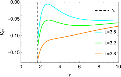
(a) KTN BH with $n_{*}=1$ and $a_{*}=1.20$ for $E=0.9$. ISCO is located at $r_{\rm ISCO}=3.6M$.

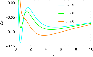
(b) KTN NS with $n_{*}=1$ and $a_{*}=1.45$ for $E=0.9$. ISCO does not exist.

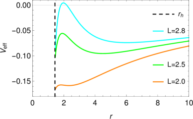
(c) Kerr BH with $a_{*}=0.90$ for $E=0.9$. ISCO is located at $r_{\rm ISCO}=2.32M$.

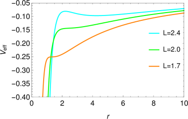
(d) Kerr NS with $a_{*}=1.05$ for $E=0.6$. ISCO is located at $r_{\rm ISCO}=0.68M$.

Figure 1: $V_{\rm eff}$ vs $r$ (in ‘$M$’) for various values of $L$ (in ‘$M$’) with the fixed $E$. $r_{h}$ indicates the radius of horizon. See section 3.1 for details.

The features of the effective potential curve of the KTN BH and KTN NS could be seen from panels (a) and (b) of figure 1, respectively. To compare it with Kerr spacetime, we can follow panels (c) and (d) of the same figure. One can see from panel (b) that the value of $V_{\rm eff}$ is finite at $r=0$ for a KTN NS and the value of $V_{0}$ can be calculated using eq. (7) but it diverges in the case of a Kerr NS (see panel (d)). Here we should note that the ISCO radii of the Kerr BH and Kerr NS have been mentioned in the plots of panels (c) and (d) of figure 1, as these values are well-known. However, the detailed studies of the locations of ISCOs in the KTN BH (panel a) and KTN NS (panel b) will be discussed in section 4. For the time-being, it could be noted (also clearly seen from the $V_{\rm eff}$ plots of panel (a)) that the ISCO occurs at $r_{\rm ISCO}=3.6M$ for the KTN BH with $n_{*}=1$ and $a_{*}=1.20$. However, one cannot determine the ISCO radius of the KTN NS with $n_{*}=1$ and $a_{*}=1.45$ from panel (b) of figure 1, as two local minima and one local maxima occur in this case. We discuss it in section 4.2.

3.2 ISCO equation from the expression of radial epicyclic frequency

One can deduce the ISCO equation directly from the expression of radial epicyclic frequency $(\Omega_{r})$. To derive the epicyclic frequencies one should investigate the small perturbations of a circular orbit. Perturbing the circular orbit with coordinate radius $r$, one can derive the radial epicyclic frequency (see eq. (11) of [34] and the discussions below of that equation). However, from the above-mentioned analysis, it is known that the square of the radial epicyclic frequency ($\Omega_{r}^{2}=0$) becomes zero at the ISCO [35, 34, 36]. No radial instability exists at the ISCO, whereas $\Omega_{r}^{2}$ becomes negative for smaller radii. The negative sign of $\Omega_{r}^{2}$ also implies that there cannot be a radial oscillation for smaller radii than the ISCO. It would be useful to mention here the general analytical expression of the epicyclic frequencies ($\omega_{x}$) in the stationary and axisymmetric spacetime, which is expressed as (see eq. (27) of [29]),

$$\omega_{x}^{2}=\left(\frac{\partial^{2}\mathcal{U_{\rm eff}}}{\partial X^{2}}\right).$$ (14)

Here $\mathcal{U_{\rm eff}}$ is the general expression of effective potential in a stationary and axisymmetric spacetime with $dX^{2}=g_{xx}dx^{2}>0$ being the proper length in the $x$ direction ($x$ denotes either radial $r$ or polar angle $\theta$ coordinate). Moreover, as $\omega_{x}$ are measured with respect to the proper time of a comoving observer, after dividing it by the squared redshift factor, one can obtain the observed epicyclic frequencies ($\Omega_{x}$) at infinity (see eqs. 32-33 of [29] and related discussions there for details). Now, it is clear from eq. (14) that the sign of $\omega_{r}^{2}$ (and also $\Omega_{r}^{2}$) is correlated with the sign of the second derivative of effective potential. However, $\Omega_{r}^{2}$ is positive for a SCO and we will show in this paper that all derived SCOs in the KTN spacetime cannot be accessible for a test particle. Rather, some SCOs cannot exist in reality and the innermost SCO is determined from the remaining SCOs.

Before going into the more detail, we should first clarify that we mainly focus on the equatorial circular orbits in this paper. Therefore, we can directly use the expressions of three fundamental frequencies which have already been deduced for KTN spacetime in [24] using the general formulation derived by Ryan [32]. These are orbital frequency ($\Omega_{\phi}$) or the Kepler frequency

$$\Omega_{\phi}=\pm\frac{m^{\frac{1}{2}}}{r^{\frac{1}{2}}~{}(r^{2}+n^{2})\pm a~{}m^{\frac{1}{2}}},$$ (15)

where $m=M~{}(r^{2}-n^{2})+2~{}n^{2}r$, and the radial ($\Omega_{r}$) and vertical ($\Omega_{\theta}$) epicyclic frequencies [24]

$$\Omega_{r} = \pm\frac{1}{(r^{2}+n^{2})\left[r^{\frac{1}{2}}~{}(r^{2}+n^{2})\pm a~{}m^{\frac{1}{2}}\right]}.\left[M(r^{6}-n^{6}+15n^{4}r^{2}-15n^{2}r^{4})-16n^{4}r^{3}\right.$$

$$\left.-2M^{2}r(3r^{4}-2n^{2}r^{2}+3n^{4})\pm 8ar^{\frac{3}{2}}m^{\frac{3}{2}}+a^{2}\left\{M(n^{4}+6n^{2}r^{2}-3r^{4})-8n^{2}r^{3}\right\}\right]^{\frac{1}{2}},$$

$$\Omega_{\theta} = \pm\frac{1}{(r^{2}+n^{2})\left[r^{\frac{1}{2}}~{}(r^{2}+n^{2})\pm a~{}m^{\frac{1}{2}}\right]}.\left[M(r^{6}-n^{6}+15n^{4}r^{2}-15n^{2}r^{4})+2n^{2}r(3r^{4}-2n^{2}r^{2}+3n^{4})\right.$$ (17)

$$\left.+16M^{2}n^{2}r^{3}\mp 4ar^{\frac{1}{2}}m^{\frac{1}{2}}(n^{2}+Mr)(n^{2}+r^{2})-a^{2}\left\{M(n^{4}+6n^{2}r^{2}-3r^{4})-8n^{2}r^{3}\right\}\right]^{\frac{1}{2}}$$

respectively. We note that the upper sign is applicable for the direct orbits and the lower sign is applicable for the retrograde orbits.

Now, setting eq. (LABEL:rktn) equal to zero, we obtain the so-called ISCO equation :

$$M(r^{6}-n^{6}+15n^{4}r^{2}-15n^{2}r^{4})-2M^{2}r(3r^{4}-2n^{2}r^{2}+3n^{4})-16n^{4}r^{3}$$

$$\pm 8ar^{\frac{3}{2}}m^{\frac{3}{2}}+a^{2}\left\{M(n^{4}+6n^{2}r^{2}-3r^{4})-8n^{2}r^{3}\right\}=0.$$ (18)

One can check that eq. (18) reduces to the ISCO equation in Kerr spacetime [37] for $n=0$ :

$$r^{2}-6Mr\pm 8ar^{\frac{1}{2}}M^{\frac{1}{2}}-3a^{2}=0$$ (19)

and obtain only one positive real root of this equation for each corresponding value of $a_{*}$ (see figure 7 of [30]), which is considered as the radius of the ISCO for that particular value of $a_{*}$. This is true for all values of $a_{*}$ whether it indicates a BH ($-1\leq a_{*}\leq 1$) or a NS ($a_{*}>1,\,\,a_{*}<-1$). One intriguing feature is that eq. (18) gives more than one positive real root for one class of combinations between $a_{*}$ and $n_{*}$. More interestingly, eq. (18) does not give any positive real root for another class of combinations between $a_{*}$ and $n_{*}$, which indicates that the so-called ISCO does not exist for these cases. We will discuss all these cases as we proceed.

4 Stable circular orbits in KTN spacetime

In this section, we study the properties of the circular geodesics of a test particle, occurred in the KTN spacetime and find the locations of the ISCO as well as the other SCOs. We divide it into two subsections.

4.1 Location of ISCO in KTN black hole

The ISCO equation (eq. 18) cannot be solved analytically, but one can solve it numerically and obtain the solutions for all possible combinations of $a_{*}$ and $n_{*}$. For the non-extremal KTN BH, we obtain only one positive real root of eq. (18) outside the horizon $r_{h}=M(1+\sqrt{1+n_{*}^{2}-a_{*}^{2}})$. Hence, we can conclude that the ISCO always occurs outside of the horizon : $r_{\rm ISCO}>r_{h}$ for all possible combinations of $a_{*}$ and $n_{*}$ which represent the non-extremal KTN BHs. This is expected.

In an extremal KTN BH, ISCO equation for the direct orbits (eq. 18) reduces to

$$M(r^{6}-n^{6}+15n^{4}r^{2}-15n^{2}r^{4})-2M^{2}r(3r^{4}-2n^{2}r^{2}+3n^{4})-16n^{4}r^{3}$$

$$+8(M^{2}+n^{2})^{\frac{1}{2}}r^{\frac{3}{2}}m^{\frac{3}{2}}+(M^{2}+n^{2})\left\{M(n^{4}+6n^{2}r^{2}-3r^{4})-8n^{2}r^{3}\right\}=0$$ (20)

and it is satisfied by $r_{1}=M$ which is independent of $n_{*}$. This also means that this solution is satisfied by all values of $n_{*}$ and coincides with the horizon $r_{1}=r_{h}=M$. We note that the ISCO equation (eq. 19) for an extremal Kerr BH is satisfied by $r=M$ and therefore, ISCO occurs at $r=M$. One intriguing feature is that eq. (20) is also satisfied by another positive real root ($r_{2}$) which occurs outside (i.e., $r_{2}>M$) or inside (i.e., $r_{2}<M$) the horizon depending on the value of $n_{*}$. For $0<n_{*}<0.577$, $r_{2}$ occurs inside the horizon whereas it occurs outside the horizon for $n_{*}>0.577$, and $r_{2}$ coincides with the horizon ($r_{1}=r_{2}=M$) for $n_{*}\approx 0.577$. As the orbits inside the horizon are unfeasible for an accreting BH, one should consider $r_{1}=M$ as the ‘physical ISCO’ for an extremal KTN BH with $n_{*}$ value of the following range, $n_{*}:0<n_{*}\lesssim 0.577$. However, referring to section 3.2, we plot the radial epicyclic frequency ($\Omega_{r}$) for a few values of $n_{*}$.

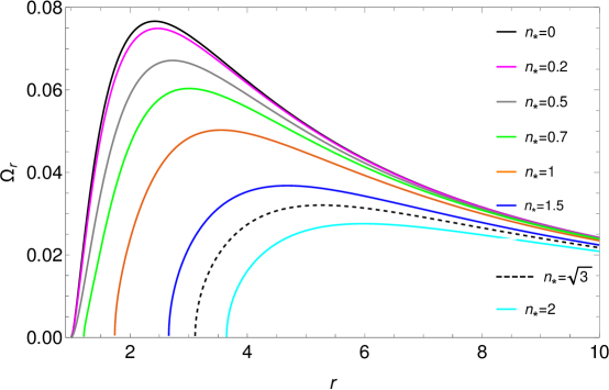
Figure 2: $\Omega_{r}$ (in ‘$M^{-1}$’) vs $r$ (in ‘$M$’) for different values of $n_{*}$ of the extremal KTN BHs. X-axis starts from the event horizon $r_{h}=M$. Solid black curve ($n_{*}=0$) stands for the extremal Kerr BH and the ISCO is located at $r_{\rm ISCO}=M$ in this case. Each curve (except the solid black, magenta and gray curves) touches the X-axis at $r=r_{2}$ which is considered as the ‘physical ISCO’ for an extremal KTN BH. Magenta and gray curves touch the X-axis at $r_{1}=M$ which is considered as the ISCO for these two cases. See section 4.1 for details.

Except solid black, magenta and gray curves, all the curves of figure 2 indicate the positions of $r_{2}$ where $\Omega_{r}$ vanishes. We note that solid black curve shows the position of ISCO for an extremal Kerr BH whereas magenta and gray curves show the position of $r_{1}=M$, as is discussed above. We confirm that $\Omega_{r}$ also vanishes at $r_{1}=M$ for all these cases. It suggests that no radial instabilities should be found at $r_{1}$ and $r_{2}$ (see the related discussions in section 3.2), in principle. However, as the values of $\Omega_{r}^{2}$ become negative between $r_{1}$ and $r_{2}$ for the extremal KTN BHs with $n_{*}>0.577$, SCOs do not exist. Now, question is which should be the ISCO ($r_{1}$ or $r_{2}$) in a realistic astrophysical situation for the extremal KTN BHs with $n_{*}>0.577$? The answer of this question, i.e., the location of ‘physical ISCO’ for the extremal KTN BH could not be found from the effective potential plot, shown in panel (a) of figure 3 (effective potential in the extremal Kerr BH is shown in panel (b) only for the comparison).

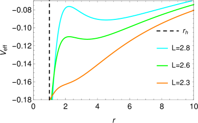
(a) KTN extremal BH with $n_{*}=1$ & $a_{*}=\sqrt{2}$ for $E=0.8$. ‘Physical ISCO’ is located at $r_{2}=1.75M$

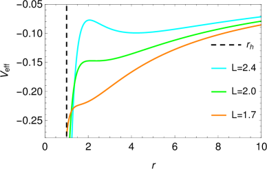
(b) Kerr extremal BH with $a_{*}=1$ for $E=0.7$. ISCO is located at $r_{\rm ISCO}=M$

Figure 3: $V_{\rm eff}$ vs $r$ (in ‘$M$’) for various values of $L$ (in ‘$M$’) with the fixed $E$. $r_{h}$ indicates the radius of horizon. See section 4.1 for details.

Therefore, to find the answer of this important question, we calculate the energy at $r_{1}$ and $r_{2}$ using eq. (12). We find that $E$ comes out as less than $1$ in all the orbits which are in the range of $r\geq r_{2}$. This indicates that all these orbits are accessible by a test particle and these are realistic for an astrophysical purpose. Now, if we calculate the energy at $r_{1}$, we obtain

$$E_{r=r_{1}=M}={\sqrt{\frac{1+n_{*}^{2}}{3-n_{*}^{2}}}}$$ (21)

and the corresponding angular momentum is

$$L_{r=r_{1}=M}=\frac{2M(1+n_{*}^{2})}{\sqrt{3-n_{*}^{2}}}.$$ (22)

At this point, we should note that all circular orbits are not bound. The orbit of a test particle with energy $E=1$ is regarded [37] as the marginally bound orbit ($r_{\rm mb}$). Therefore, the bound circular orbits exist for $r>r_{\rm mb}$ with $E<1$, whereas unbound circular orbits exist for $r<r_{\rm mb}$ with $E>1$ [33]. If an infinitesimal outward perturbation is given, a test particle in an unbound orbit escapes to infinity on an asymptotically hyperbolic trajectory. However, in realistic astrophysical problems, particle infall from infinity is very nearly parabolic, and any parabolic trajectory, penetrating to $r<r_{\rm mb}$, must plunge directly into the collapsed object [33]. Now, we can see from eq. (21) that $E\geq 1$ at $r=r_{1}$ for $1\leq n_{*}<\sqrt{3}$, and $E<1$ for $n_{*}<1$. Therefore, the single orbit which occurs at $r=r_{1}=M$ could not be important in a realistic astrophysical situation for $1<n_{*}<\sqrt{3}$, as the particle will plunge directly into the black hole from the $r_{2}$ orbit. Therefore, we should identify $r=r_{2}$ as the ISCO in this case.

For $0.577<n_{*}\leq 1$, the $r=r_{1}$ orbit must be a SCO in principle and it should exist but it could not be relevant for the astrophysical purpose. Let us first consider that an extremal KTN BH with $0.577<n_{*}\leq 1$ is accreting matter from a distant source. The matter generally follows the SCOs and the accretion disk exists till $r=r_{\rm ISCO}$. The accreting matter free-falls towards the BH at $r<r_{\rm ISCO}$, as no SCOs exist there. It is clear from figure 2 that SCOs exist for $r\geq r_{2}$ (as $\Omega_{r}^{2}\geq 0$) and no SCOs exist in this range $r_{1}<r<r_{2}$ (as $\Omega_{r}^{2}<0$). In such a situation, one cannot expect that the accreting matter will form a ‘single-ring’ disk on the event horizon, i.e., $r=r_{1}=M$ after a free-fall from $r>r_{2}$ to $r=r_{1}$ which basically represents the boundary of the BH. Therefore, one should consider $r=r_{2}$ as the ‘physical ISCO’ for all practical purposes in the case of an extremal KTN BH with $n_{*}>0.577$. Figure 2 also reveals that the radius of ISCO ($r_{2}$ in this case) increases with increasing the value of $n_{*}$ of the extremal KTN BHs with $n_{*}>0.577$. However, as we have already discussed, $r_{1}$ should be the ‘physical ISCO’ for an extremal KTN BH with $0<n_{*}\lesssim 0.577$.

4.2 Location of ISCO in KTN naked singularity

As the so-called ISCO equation (eq. 18) could not be solved analytically, we solve it numerically and obtain three classes of solution. For one class of solution, we obtain two positive real roots ($r_{1}$ and $r_{2}$) of eq. (18). For the second class, one can obtain one (double root) positive real root, and for another class, no positive real roots are found. Basically, in the second class of solution, two positive real roots become equal, i.e., $r_{1}=r_{2}$ for some special combinations of $a_{*}$ and $n_{*}$. Our result has been depicted in figure 4. It shows that one cannot obtain any positive real root of eq. (18) for those combinations of $a_{*}$ and $n_{*}$, which are fallen in the red region, whereas at least one positive real root can be obtained, if one choses the values of $a_{*}$ and $n_{*}$ from the white region. In this sense, the ISCO should not exist for the KTN NSs which are in the ‘red-coloured’ region and SCOs can exist everywhere in this spacetime. Here, we should note that, considering a toy model of a static spherically symmetric perfect fluid interior with a singularity at the origin, it was found [38] that the SCOs exist everywhere (till $r\rightarrow 0$).

Figure 4: NUT parameter ($n_{*}$) versus Kerr parameter ($a_{*}$) space, which is divided into a KTN BH and KTN NS region by the thin black curve. The $a_{*}$ and $n_{*}$ values of each point in the thin black curve also indicates an extremal KTN BH. Solving eq. (18) one cannot obtain a positive real root, for those combinations of $a_{*}$ and $n_{*}$ which are fallen in the ‘red-coloured’ region, whereas at least one positive real root can be obtained, if one choses the combinations of $a_{*}$ and $n_{*}$ from the ‘white-coloured’ region. One should note that the ‘red-coloured’ region does not include any KTN BH. Because, solving eq. (18) one can always obtain at least one positive real root outside or on the horizon for all KTN BHs. See sections 4.1 and 4.2 for details.

However, our case is completely different here, which we will be discussing in this section considering the various scenarios. Let us first consider an example.

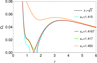
(a) Different of $\Omega_{r}$ curves shows that the locations of SCOs are highly affected with a slight change in the Kerr/NUT parameter values. As an example, $a_{*}$ changes its value with a fixed $n_{*}$ in this particular figure.

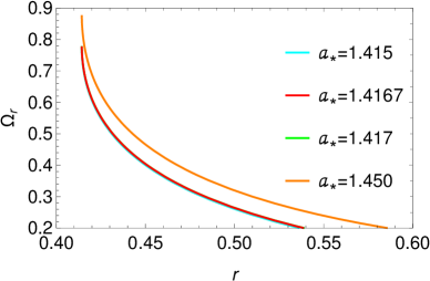
(b) Zoomed version of panel (a) with range $0.4\leq r/M\leq 0.6$ is shown for clarity. $\Omega_{r}$ curves are discontinued in the region : $r<0.414M$.

Figure 5: $\Omega_{r}$ (in ‘$M^{-1}$’) vs $r$ (in ‘$M$’) for various values of $a_{*}$ with $n_{*}=1$. Panel (a) also clearly shows that three classes of solution (two, one and zero positive roots) of the ISCO equation (eq. 18) exist for KTN NS. The orange and green curves show that one cannot obtain a positive real root by solving of eq. (18) as $\Omega_{r}$ does not vanish in any orbit. But, one can obtain two positive real roots for the cyan curve and one positive real root for the red curve. Actually, the last one is the double root, i.e., two positive real roots coincide at $r/M=1.5$ for $a_{*}=1.4167$, which is clear from this figure. See section 4.2 for details. For completeness, the black dashed curve is added, which stands for an extremal KTN BH. We have already discussed on it in section 4.1

.

In figure 5, we have plotted $\Omega_{r}$ for different values of $r$. It shows that the black dashed curve which stands for the extremal KTN BH ($n_{*}=1,a_{*}=\sqrt{2}$) touches the X-axis at $r/M=1.75$, which means that eq. (18) has a positive real root at $r/M=1.75$. It has already been recognized as $r_{2}$ or the ‘physical ISCO’ for this case (see also the solid orange curve in figure 2 and the related discussion in section 4.1). Now, if we slightly increase the value of $a_{*}$ from $\sqrt{2}$ to $1.415$ fixing the value of $n_{*}=1$, the event horizon vanishes and we should consider it as a KTN NS. In this case, the solid cyan curve of figure 5 touches the X-axis twice at $r_{1}/M=1.2$ and $r_{2}/M=1.7$ respectively. This means that eq. (18) has two positive real roots at $r_{1}$ and $r_{2}$. If we again increase the value of $a_{*}$ from $a_{*}=1.415$ to $a_{*}=1.4167$, the two roots become equal and coincide at $r_{1}=r_{2}=1.5$. This means, that one can obtain only one positive real root in this particular case. This is shown by the solid red curve in figure 5. The green and orange curves do not touch the X-axis, which means that one cannot obtain any positive real root of eq. (18) for these two curves, i.e., for $n_{*}=1$ & $a_{*}=1.417$ and $n_{*}=1$ & $a_{*}=1.45$, respectively. As we have discussed in section 3.2, one can think that SCOs exist for all those values of $r$ which gives the positive $\Omega_{r}$ values in principle. It can easily be seen that the SCOs exist in the outer branch ($r_{2}\leq r<\infty$) of the cyan curve but for the inner branch ($r\leq r_{1}$) it might not be true always. We will discuss it in the next two sections. A close look of panel (b) (the zoomed version of panel (a) of figure 5) reveals that the cyan, red, green and orange curves (which are for KTN NSs) do not continue to $r\rightarrow 0$. Rather, all these curves are discontinued after arriving at a particular orbit of radius $r=R_{f}$. Mathematically, this discontinuation indicates that the value of $\Omega_{r}$ becomes imaginary in the region : $r<R_{f}$, which is unphysical. One can check that the Kepler frequency (eq. 15) vanishes at the orbit $r=R_{f}$, which is unexpected. As far as we know, this special feature has not been seen in other spacetimes until now. Therefore, we should discuss it in detail in the next section. Side by side, we also continue our discussion on SCOs in the later sections.

4.2.1 Digression 1 : Forbidden region for a test particle moving in a circular geodesic

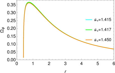
Figure 6: $\Omega_{\phi}$ (in ‘$M^{-1}$’) vs $r$ (in ‘$M$’) for various values of $a_{*}$ with $n_{*}=1$. One intriguing feature is that $\Omega_{\phi}$ vanishes at $r=0.414M$. See section 4.2.1 for details.

Figure 6 shows that the Kepler frequency of a test particle which moves in a circular geodesic, increases at first, attains a peak value at $r=r_{p}$ and then vanishes at a particular orbit of radius $r=R_{f}$. The value of $R_{f}$ can be obtained setting the numerator of eq. (15) as zero and it gives

$$R_{f}=M\left(n_{*}\sqrt{1+n_{*}^{2}}-n_{*}^{2}\right).$$ (23)

Therefore, a test particle moving in a circular geodesic cannot continue its motion at $r<R_{f}$ as its angular velocity is zero. We call it as the forbidden region. As the angular velocity vanishes at $r=R_{f}$, the test particle should free-fall towards the central object. In the next sections, we will show that the test particle cannot even continue its stable circular motion till $r\rightarrow R_{f}$, in a realistic situation. However, we can see from eq. (23) that the forbidden region is fully controlled by the gravitomagnetic monopole $n_{*}$ and Kerr parameter ($a_{*}$) has no influence on it. Therefore, this region is absent in the Kerr spacetime, i.e, $R_{f}=0$ (see figure 7).

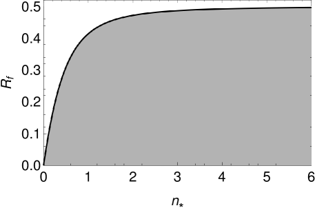
Figure 7: $R_{f}$ (in ‘$M$’) vs $n_{*}$, where Gray region indicates the “Forbidden Region” : $r<R_{f}$. The solid black curve indicates the boundary values of the forbidden region, for each corresponding value of $n_{*}$. $\Omega_{\phi}$ vanishes on the solid black curve. See section 4.2.1 for details.

If $n_{*}$ increases from $0$ to a higher value, the radius of the forbidden region increases primarily but it cannot be greater than $M/2$. A short calculation reveals that

$$\frac{R_{f}}{M}|_{n_{*}>>1}\approx n_{*}^{2}\left(1+\frac{1}{2n_{*}^{2}}\right)-n_{*}^{2}=\frac{1}{2}$$ (24)

for higher values of $n_{*}$. It means that for $n_{*}>>1$, the higher order terms could be neglected and the radius of the forbidden region becomes almost a constant : $M/2$ which is also clear from figure 7. The gray region indicates the forbidden region for various values of $n_{*}$. As $R_{f}$ is always less than $r_{h}$, i.e., $R_{f}<r_{h}$, it remains hidden inside the horizon and this region could only be meaningful in case of a KTN NS. For a particular value of $n_{*}$, the Kepler frequency not only vanishes at $R_{f}$ in the strong gravity regime , but the other two fundamental frequencies (radial and vertical epicyclic frequencies) are also discontinued there, acquiring the finite values. This implies that the circular motion become frozen in the region $r<R_{f}$ and cannot be accessed by a test particle with its circular geodesic motion. Mathematically, all three fundamental frequencies $(\Omega_{\phi},\Omega_{\theta}$ and $\Omega_{r})$ become imaginary at $r<R_{f}$.

However, differentiating eq. (15) with respect to $r$ and setting it to zero :

$$\frac{d\Omega_{\phi}^{\rm KTN}}{dr}=\frac{-8n^{2}r^{3}+M\left(n^{4}+6n^{2}r^{2}-3r^{4}\right)}{2\sqrt{rm}\left[\sqrt{r}(r^{2}+n^{2})+a\sqrt{m}\right]^{2}}|_{r=r_{p}}=0$$ (25)

one can obtain the radius of the peak ($r=r_{p}$) where the Kepler frequency acquires the maximum value

$$r_{p} = \frac{Mn_{*}}{3}\left[\left(6+8n_{*}^{2}+3\left(1+n_{*}^{2}\right)^{1/3}+\frac{2n_{*}\left(9+8n_{*}^{2}\right)}{\left[3+4n_{*}^{2}-3(1+n_{*}^{2})^{1/3}\right]^{\frac{1}{2}}}\right)^{\frac{1}{2}}\right.$$ (26)

$$\left.-\left(3+4n_{*}^{2}-3(1+n_{*}^{2})^{1/3}\right)^{\frac{1}{2}}-2n_{*}\right].$$

Eq. (26) shows that the value of $r_{p}$ also does not depend on $a_{*}$ and therefore the similar situation cannot arise in case of a Kerr NS by any means.

Conclusion drawn from this discussion : The above discussion compels us to conclude that the SCOs do not exist in the region: $r\leq R_{f}$ for all those four NS curves of figure 5.

4.2.2 Digression 2 : Angular velocity of the test particle inside the ergoregion

Now, the question is : can the SCOs exist in the range $R_{f}<r\leq r_{1}$ for the cyan curve and $R_{f}<r<\infty$ for the red, green and orange curve of figure 5(a)?

Here, we recall eq. (3) where $r_{e}$ represents the boundary of the ergoregion. Though the horizon does not exist for the KTN NS, the ergoregion remains there, and its radius becomes

$$r_{e}|_{\theta=\pi/2}=M\left(1+\sqrt{1+n_{*}^{2}}\right).$$ (27)

For KTN spacetime it depends on the value of $n_{*}$ which is seen from eq. (27). We note that the radius of ergoregion at the equatorial plane remains same ($r_{e}|_{\theta=\pi/2}=2M$) for all values of $a_{*}$, whether it is a Kerr BH or a Kerr NS [27]. However, it is well-known that it is impossible to stay fixed inside the ergoregion with some arbitrary velocities. In general, it is possible for an observer (or the test particle) to fix at a point $(r,\theta)$ inside the ergoregion, if it rotates (prograde only) inside the ergoregion [1, 42] with the angular velocity $\Omega$ : $\Omega_{-}<\Omega<\Omega_{+}$. This range is determined by using eqs. (21-23) of [30] :

$$\Omega_{\pm}=\frac{2a\left(n^{2}+Mr\right)\pm\left(n^{2}+r^{2}\right)\sqrt{\Delta}}{\left(n^{2}+r^{2}\right)^{2}+a^{2}\left[3n^{2}+r(2M+r)\right]}.$$ (28)

Therefore, inside the ergoregion, a test particle can rotate in an SCO with the Kepler frequency $\Omega_{\phi}$, if and only if it satisfies the following condition :

$$\Omega_{-}<\Omega_{\phi}<\Omega_{+}.$$ (29)

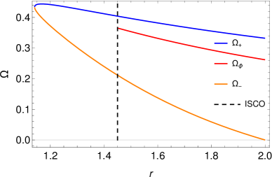
(a) Kerr BH with $a_{*}$=0.99

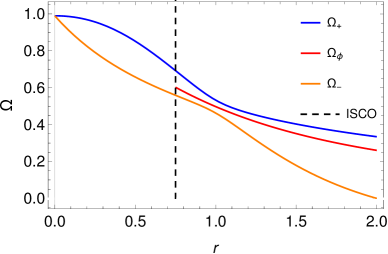
(b) Kerr NS with $a_{*}$=1.01

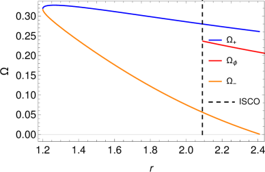
(c) KTN BH with $n_{*}=1$ and $a_{*}=1.4$

(d) KTN NS with $n_{*}=1$ and $a_{*}=1.415$ (corresponds to the cyan curve of figure 5)

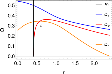
(e) KTN NS with $n_{*}=1$ and $a_{*}=1.45$ (corresponds to the orange curve of figure 5)

Figure 8: Inside the ergoregion, a test particle can take only those $\Omega$ values which are in the following range : $\Omega_{-}<\Omega<\Omega_{+}$. $\Omega_{+}$ and $\Omega_{-}$ (in ‘$M^{-1}$’) are shown as solid blue and orange curves, respectively, and have been plotted specifically inside the ergoregion, in the equatorial plane ($\theta=\pi/2$), as a function of $r$ (in ‘$M$’). For BHs, we can see from panels (a) and (c) that $\Omega_{\pm}$ meet at the horizon. For Kerr NS, we can see from panels (b) that $\Omega_{\pm}$ meet at the singularity ($r=0$) but they never meet in the case of KTN NSs (see panels (d) and (e)). The red solid curves represent the Kepler frequency $\Omega_{\phi}$ which does not satisfy eq. (29) after reaching the point ‘C’, for the KTN NSs. We note, as no SCOs exist in the range $r_{1}<r<r_{2}$ in panel (d), $\Omega_{\phi}$ is meaningless in this region. See section 4.2.2 for details.

It is seen from panels (a) and (b) of figure 8 that this condition (eq. 29) is always satisfied in the cases of Kerr BH and Kerr NS. Panel (c) shows that it is also satisfied in the case of a KTN BH but the condition mentioned in eq. (29) cannot be satisfied in the case of a KTN NS (see panels (d) and (e)). This is because, it is clearly seen from panels (d) and (e) that when the test particle reaches at the orbit of radius $r_{\rm C}$ (which corresponds to the point ‘C’ of the plots drawn in panels (d) and (e) of figure 8), it coincides with the $\Omega_{-}$ curve. Equating the expressions of $\Omega_{\phi}=\Omega_{-}$, one can numerically obtain the value of $r_{\rm C}$. Remarkably, $r_{\rm C}$ coincides with the circular photon orbit (CPO) or $r_{c}$ ($r_{\rm C}\equiv r_{c}$) for every combination of $a_{*}$ and $n_{*}$ which represents a KTN NS. The reason behind that is, $\Omega_{-}$ is associated with the null vector $K_{-}=\partial_{t}+\Omega_{-}\partial_{\phi}$, as was pointed out in eqs. (29–30) of [30]. However, a test particle which moves in a timelike circular orbit, unable to make its four-velocity $u$ become null at $r_{\rm C}$. Therefore, the SCOs which exist in the range : $r\leq r_{\rm C}$, cannot be accessible by a test particle with its Kepler frequency. It would immediately fall into the KTN collapsed object and hence, the SCOs of $r\leq r_{\rm C}$ are not meaningful.

We may note here that $\Omega_{\pm}$ meet at the horizon and become a single-valued function ($\Omega_{h}$), in case of a Kerr as well as a KTN BH. This frequency for the KTN BH can be written as

$$\Omega_{h}=\frac{a}{2(Mr_{h}+n^{2})}.$$ (30)

It reduces to

$$\Omega_{h}^{\rm Kerr}=\frac{a}{2Mr_{h}^{\rm Kerr}}$$ (31)

(where $r_{h}^{\rm Kerr}/M=1+\sqrt{1-a_{*}^{2}}$ ) in the Kerr BH, which is well-known. For Kerr NS, $\Omega_{\pm}^{\rm Kerr}$ meet at the singularity ($r=0$) with $\Omega_{\pm}|_{r=0}=1/a$ [30], but for KTN NS $\Omega_{\pm}$ take two different values at $r=0$ :

$$\Omega_{\pm}|_{r=0}=\frac{2a\pm\sqrt{a^{2}-n^{2}}}{n^{2}+3a^{2}}$$ (32)

which is seen from panels (d) and (e) of figure 8. We note that the condition $a^{2}-n^{2}>1$ holds for the KTN NS and therefore, we always obtain two values of $\Omega_{\pm}$ at $r=0$.

Conclusion drawn from this discussion : The above discussion tells us that a test particle cannot access the SCOs which exist in the region : $r\leq r_{\rm C}$ ($r_{\rm C}$ corresponds to the circular photon orbit) for all four NS curves of figure 5. Therefore, the ‘physical ISCO’ should exist in the region : $r>r_{\rm C}$ and its exact location is obtained in the next section.

4.2.3 Energy of the SCOs

Figure 9: Energy $E$ vs $r$ (in ‘$M$’) for $n_{*}=1$ with different values of $a_{*}$. The four dashed straight lines (cyan, red, green and orange) are the corresponding $r_{\rm C}$ values ($r_{\rm C}/M=0.66,\,\,0.654,\,\,0.65,\,\,0.58$) of the cyan, red, green and orange curves, respectively. Magenta and black dashed straight lines show the positions of $r_{1}$ and $r_{2}$ respectively, which arise only for the solid cyan curve. Note that the cyan curve has actually no meaning in the region $r_{1}<r<r_{2}$, as no SCOs exist in this region. In case of the solid red curve, $r_{1}$ coincides with $r_{2}$, i.e., $r_{1}=r_{2}$, which is represented by the dot-dashed red straight line. See sections 4.2.3 and 4.2.4 for details.

Increasing the energy $E$ with decreasing $r$ is one of the consequences of the absence of stable orbits [38]. One can check it in the region $r_{1}<r<r_{2}$ for the cyan curve of figure 9, but, as $E$ decreases with decreasing of $r$ in the region $r<r_{1}$, we can conclude that SCOs exist in that region. Now, the cyan curve shows a sudden fall of $E$ for $r/M\sim 1.1$ and the test particle acquires $E=0$ at $r=r_{0}/M\approx 0.99$. $E=0$ represents that the efficiency $(1-E)$ of accretion reaches $100\%$ at $r=r_{0}$ orbit, i.e., all the mass-energy of the accreting gas is converted to radiation and returned to infinity (see second paragraph of section 3.2 of [38]). This implies a perfect engine which converts mass into energy with $100\%$ efficiency [38]. Hence, the SCOs at $r/M<0.99$, which have negative $E$ values, are not meaningful. Therefore, in such a case, one can choose $r=r_{0}$ as the ‘physical ISCO’.

Figure 9 is drawn for $n_{*}=1$ with different values of $a_{*}$. As is shown in this figure, $r_{\rm C}/M$ arise at $0.654,0.65$ and $0.58$ for the red, green and orange curves, respectively. These are also far from the $E=0$ orbit ($r_{0}/M$) which occur at $0.9963,0.9960$ and $0.95$ respectively for these three curves. Remarkably, one can see from figure 5(a) and figure 9 that there is no discontinuity in these three curves (including the solid red one), i.e., $E$ decreases with decreasing of $r$ in the whole range : $r_{0}\leq r\leq\infty$ and becomes zero at $r=r_{0}$. Therefore, although one positive real root is obtained (by solving the so-called ISCO equation) at $r_{1}=r_{2}=1.5M$ (red dot-dashed straight line) for the solid red curve, this may be ignored, and we can conclude that the ‘physical ISCO’ occurs at $r=r_{0}$ in all these three cases. Here, we should remember that these ISCOs do not carry the usual meaning which we have discussed in section 3, as these new ISCO radii do not satisfy the so-called ISCO equation (eq. 18). However, these new ISCO radii must satisfy the SCO condition mentioned in section 3. One important thing is that there could exist many combinations of $a_{*}$ and $n_{*}$ (those are mainly fallen in the ‘red-coloured’ region of figure 4), for which the accretion efficiency reaches $100\%$ for the KTN NSs, whereas it is possible only for those Kerr NSs whose $a_{*}$ values are in the following range: $1<a_{*}\leq\sqrt{32/27}$. As an example, for $a_{*}=\sqrt{32/27}\approx 1.089$, accretion efficiency reaches $100\%$ at the ISCO : $r_{\rm ISCO}=2M/3$ [43] ($E$ becomes zero in this particular orbit, see [37, 44]).

4.2.4 Importance of the marginally bound orbit

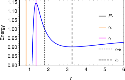
(a) Energy $E$ vs $r$ (in ‘$M$’)

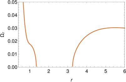
(b) $\Omega_{r}$ (in ‘$M^{-1}$’) vs $r$ (in ‘$M$’)

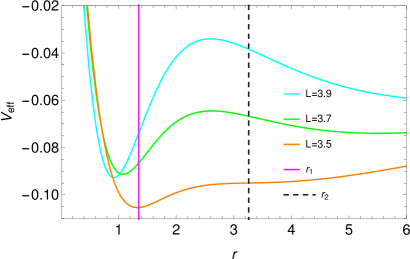
(c) $V_{\rm eff}$ vs $r$ (in ‘$M$’) for various values of $L$ (in ‘$M$’) with $E=0.9$.

Figure 10: Panel (a) shows the positions of various orbits for a KTN NS with $n_{*}=1.84$ and $a_{*}=2.10$ : $R_{f}/M=0.47$, $r_{\rm C}/M=0.82$, $r_{1}/M=1.35$, $r_{2}/M=3.26$ and $r_{\rm mb}/M=1.81$. Note that the blue energy curve has no meaning in the region $r_{1}<r<r_{2}$, as no SCOs exist in this region, which is seen from panel (b). However, it is necessary to show the location of $r_{\rm mb}$. Panel (c) shows the behaviour of effective potential. See section 4.2.4 for details.

Energy $E$ can increase or decrease with $r$ and depending on that one can find the location of SCOs. It is seen from figure 9 that the value of $E$ always remains less than $1$ in all orbits for all curves. As we have discussed in section 4.1 that an orbit is called marginally bound ($r_{\rm mb}$), if its energy becomes $1$. Now, setting $E=1$ in eq. (12), one can numerically solve the following expression

$$(r^{2}+n^{2})\left(r^{3}-3Mr^{2}-3n^{2}r+Mn^{2}+2a(mr)^{\frac{1}{2}}\right)-\left[r^{\frac{1}{2}}(r^{2}-2Mr-n^{2})+am^{\frac{1}{2}}\right]^{2}=0$$

(33)

to obtain the radius ($r_{\rm mb}$) of the marginally bound orbit. It is difficult to solve analytically for the KTN spacetime but can be solved for the Kerr BH, which gives [45] (see eq. 141 of Chapter 7 of [37] also)

$$r_{\rm mb}^{\rm Kerr}=M\left(2-a_{*}+2\sqrt{1-a_{*}}\right)$$ (34)

for the direct orbits. One can check that the value of $r_{\rm mb}^{\rm Kerr}$ always comes as less than the value of $r_{\rm ISCO}^{\rm Kerr}$ for a particular value of $a_{*}$ in case of the Kerr spacetime. For the extremal Kerr BH, $r_{\rm ISCO}^{\rm Kerr}$ and $r_{\rm mb}^{\rm Kerr}$ coalesce at the horizon : $r_{h}/M=1$. That is why, we generally do not bother about $r_{\rm mb}^{\rm Kerr}$ for the realistic astrophysical problems in Kerr BH and deal only with the $r_{\rm ISCO}^{\rm Kerr}$.

Let us now consider figure 10 which is a special case in KTN spacetime. This figure corresponds to a KTN NS with $n_{*}=1.84$ and $a_{*}=2.10$. One can safely say from panel (b) of figure 10 that the SCOs do exist in the outer branch, i.e., $r_{2}/M\geq 3.26$. Panel (a) also shows that $E$ of a test particle decreases with $r$ until it reaches at $r_{2}/M=3.26$, whereas SCOs do not exist for the range $1.35<r/M<3.26$ as $E$ increase with $r$. This is also clear from panel (b). However, $r_{\rm mb}$ is located at $r_{\rm mb}/M=1.81$ and it palys an importnat role in such a situation. After reaching at $r=r_{2}$, the test particle should start to free-fall in principle and reach at the $r=r_{1}=1.35M$ orbit, the feature of which is a bit similar to the cyan curve of figure 9. Incidentally, the energy of the $r_{1}$ orbit is greater than $1$ in this particular case, i.e., $E|_{r=r_{1}}>1$, which is seen from panel (a) of figure 10. Moreover, one can also notice that the test particle faces the ‘unbound’ ($E>1$) orbits even in the region : $r_{1}<r<r_{\rm mb}$ before reaching at $r=r_{1}$. Therefore, as the test particle penetrates to the unbound circular orbits ($E>1$) at $r<r_{\rm mb}$, it must plunge directly into the collapsed object [33] after crossing the $r=r_{\rm mb}$ orbit. Therefore, the SCOs which occur at $r\leq r_{1}$ cannot be feasible at all and these orbits are also not meaningful for the accretion disk theory. In such a situation, $r_{2}$ should be considered as the ‘physical ISCO’ and the inner branch is unfeasible.

4.3 Special case

One can see from figure 9 that the value of $r_{0}$ comes as smaller than the value of $r_{2}$, i.e, $r_{0}<r_{2}$. In this section, we show that this is not always true. Let us consider figure 11. Panels (a)-(c) of the same are drawn for three different values of $a_{*}=1.01,1.10$ and $1.30$ with the $n_{*}$ values are almost close to zero, i.e., $n_{*}=0.01,0.10$ and $0.14$. In each panel, the three dotted and dashed straight lines (black, gray, purple) are the corresponding $r_{1}$ and $r_{2}$ values of the black, gray and purple solid curves respectively, which represent energy of the circular orbits. One can see that feature of the three solid energy curves of panel (a) of figure 11 is completely different from the feature of the energy curves of figures 9 and 10(a). In figure 11, each energy curve not only crosses $E=0$ axis for three different values of $r$ (say, $r_{01},r_{02}$ and $r_{03}$, such that $r_{01}<r_{02}<r_{03}$), but also one of them ($r_{03}$) appears before $r_{2}$, i.e., $r_{2}<r_{03}$. Now, consider a test particle/accreting matter approaches to a KTN NS of $a_{*}=1.01$ and $0<n_{*}\lesssim 0.142$ from infinity (in principle). It is needless to say that it encounters $r=r_{03}$ orbit first instead of $r=r_{2}$ orbit unlike the cyan curve of figure 9. As all the mass-energy of the accreting gas is converted to radiation and returned to infinity [38] from this $r=r_{03}$ orbit, no orbits with $r<r_{03}$ are feasible in these cases. Therefore, $r=r_{03}$ should be considered as the ‘physical ISCO’ for all these three cases of panel (a) of figure 11, i.e., $r_{03}/M=0.97,0.98$ and $0.99$ for black, gray and purple solid curves respectively. Here, we should note that $n_{*}\geq 0.142$ with $a_{*}=1.01$ represent KTN BHs and one has to follow the discussion of section 4.1 to determine the location of ISCO for those cases.

Now, if we increase the value of $a_{*}$ from $1.01$ to $1.10$ (without changing the values of $n_{*}$), the special feature of the energy curves of figure 11(a) starts to disappear (see panel (b)) depending on the values of $n_{*}$ and it completely disappears for higher values of $a_{*}$ which can be seen from panel (c). We can see from panel (b) of figure 11 that although the solid purple curve crosses the $E=0$ axis thrice (similar to the solid curves of panel (a)), the gray and black curves cross the same only once (similar to the solid curves of figure 9). This is also clear from panel (d) of figure 11, which is the zoomed version of panel (b). Therefore, if a test particle/accreting matter approaches to a KTN NS of $a_{*}=1.10$ and $n_{*}=0.14$ (purple curve) from infinity (in principle), it first encounters $r_{03}/M=0.72$ (see, $r_{03}>r_{2}$) orbit which should be the ‘physical ISCO’ as is described in the previous paragraph. A new solid red curve is added in panel (d) for the KTN NS of $n_{*}=0.1164$ and $a_{*}=1.10$ to show that $r_{03}$ coincides with $r_{02}$ and $r_{2}$ at $r/M=0.651$ (i.e., $r_{03}=r_{02}=r_{2}=0.651M$, the red dot-dashed straight line) which should be considered as the ‘physical ISCO’ in this case. However, the characteristic of solid gray curve of panel (b) and the solid purple curve of panel (c) of figure 11 is similar to the solid cyan curve of figure 9. Therefore, one should consider the $E=0$ orbit (i.e., $r_{0}/M=0.11$ and $r_{0}/M=0.14$ respectively) as the ‘physical ISCO’ in these two cases. The characteristic of the gray curve of panel (c) resembles to the solid blue curve of figure 10(a) and one should consider $r_{2}/M=0.73$ as the ‘physical ISCO’ in this case. One can see that the two solid black curves of panels (b) and (c) of figure 11 continue to very close to $r=0$ and $r_{1}$ (i.e., dotted black straight lines) occurs just outside of it. The characteristic of these two curves are also similar to the solid blue curve of figure 10(a) and $r=r_{2}$ is considered as the ‘physical ISCO’, as discussed in section 4.2.4.

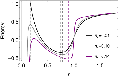
(a) $a_{*}=1.01$

(b) $a_{*}=1.10$

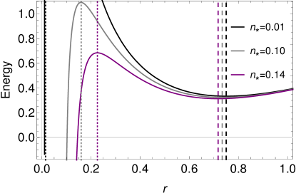
(c) $a_{*}=1.30$

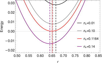
(d) Zoomed version of panel (b) with range $0.50<r/M<0.85$ is shown for clarity. A new solid red curve is added for $n_{*}=0.1164$ to show that $r_{03}$ coincides with $r_{02}$ and $r_{2}$ (i.e., $r_{03}=r_{02}=r_{2}=0.651M$, the red dot-dashed straight line) in this particular case.

Figure 11: Energy $E$ vs $r$ (in ‘$M$’) for various values of $a_{*}$ with $n_{*}$ values close to zero. In each panel, the three dotted and dashed straight lines (black, gray, purple) are the corresponding $r_{1}$ and $r_{2}$ values of the black, gray and purple solid curves respectively, which represent the orbital energy. Although the $r_{C}$ values have not been shown in these plots, one can note that $r_{C}$ appears as $r_{C}<r_{1}$ in all these cases. See section 4.3 for details.

5 Circular photon orbits

In this section, we study the location of the circular photon orbit in KTN spacetime, for completeness. The expressions of $L$ and $E$ (eqs. 12-13) imply that the circular orbits exist down in a particular orbit of radius $r=r_{\rm c}$ which is the solution of the following equation

$$r_{\rm c}^{3}-3Mr_{\rm c}^{2}-3n^{2}r_{\rm c}+Mn^{2}+2a(m_{\rm c}r_{\rm c})^{\frac{1}{2}}=0$$ (35)

where $m_{\rm c}=M~{}(r_{\rm c}^{2}-n^{2})+2~{}n^{2}r_{\rm c}$. Specifically, $E$ becomes infinity at $r=r_{\rm c}$ and hence the solution of eq. (35) gives the radius of CPO $r=r_{\rm c}$. Eq. (35) is difficult to solve analytically but we can easily solve it numerically.

5.1 CPOs in KTN black holes

One can obtain only one positive real root of eq. (35) outside the horizon in case of a non-extremal KTN BH ($a_{*}<\sqrt{1+n_{*}^{2}}$), which implies that only one CPO occurs for each corresponding combinations of $a_{*}$ and $n_{*}$ and the CPO must exists outside the event horizon.

In case of an extremal KTN BH $\left(a_{*}=\sqrt{1+n_{*}^{2}}\right)$ horizon occurs at $r_{h}=M$ and the expression (eq. 35) of CPO with radius $r_{\rm cx}$ reduces to

$$r_{\rm cx}^{3}-3Mr_{\rm cx}^{2}-3n^{2}r_{\rm cx}+Mn^{2}+2\sqrt{m_{\rm cx}r_{\rm cx}(M^{2}+n^{2})}=0$$ (36)

where, $m_{\rm cx}=M~{}(r_{\rm cx}^{2}-n^{2})+2~{}n^{2}r_{\rm cx}$. The analytical solutions of the above equation are

$$r_{\rm cx} = M,\,\,M\left(1\pm\sqrt{1+n_{*}^{2}}+\sqrt{2}\sqrt{1+n_{*}^{2}\pm\sqrt{1+n_{*}^{2}}}\right),$$ (37)

$$M\left(1\pm\sqrt{1+n_{*}^{2}}-\sqrt{2}\sqrt{1+n_{*}^{2}\pm 1\sqrt{1+n_{*}^{2}}}\right)$$

of which

$$r_{\rm cx}^{1}=M$$

and,

$$r_{\rm cx}^{\mp}=M\left(1\mp\sqrt{1+n_{*}^{2}}+\sqrt{2}\sqrt{1+n_{*}^{2}\mp\sqrt{1+n_{*}^{2}}}\right)$$ (38)

are positive and hence these are acceptable. One of these occurs at $r_{\rm cx}^{1}=M$ due to the prograde rotation whereas $r_{\rm cx}^{+}$ occurs due to the retrograde rotation. A short calculation reveals that the $r_{\rm cx}^{-}$ occurs inside the event horizon ($r_{\rm cx}^{-}<r_{h}=M$) for $n_{*}<\sqrt{3}$ (i.e., $a_{*}<2$) but it occurs outside of the event horizon for $n_{*}>\sqrt{3}$ (i.e., $a_{*}>2$). This means that two CPOs could exist simultaneously for $n_{*}>\sqrt{3}$, whereas one can neglect $r_{\rm cx}^{-}$ for $n_{*}<\sqrt{3}$, as it occurs inside the event horizon. In this special case ($n_{*}>\sqrt{3}$), one CPO coincides with the event horizon and the other one exists outside of $r_{h}$. For $n_{*}=\sqrt{3}$ (i.e., $a_{*}=2$), $r_{\rm cx}^{1}=r_{\rm cx}^{-}=M$, hence, only one CPO occurs in this case. One can check that $r_{\rm cx}^{-}$ becomes $0$ for $n_{*}=0$. That is why, we cannot obtain two CPOs for the extremal Kerr BH.

5.2 CPOs in KTN naked singularities and comparison with Kerr spacetime

For each corresponding combinations of $a_{*}$ and $n_{*}$, we always obtain only one positive real root of eq. (35) in case of a KTN NS, and it occurs at $0<r_{c}<M$.

It could be useful to mention here the location of corotating CPOs in Kerr spacetime for comparison. For a Kerr BH ($0<a_{*}\leq 1$), one can calculate the radius of the corotating CPO as $3M>r_{\rm c}^{\rm Kerr}\geq M$ using the following equation [37, 46] :

$$r_{\rm c}^{\rm Kerr}=2M\left[1+\cos\left\{\frac{2}{3}\cos^{-1}\left(-a_{*}\right)\right\}\right].$$ (39)

The corotating CPO does not occur in case of a Kerr NS (CPO is formally located at the ring singularity) [47] but remarkably it occurs for a KTN NS at $0<r_{c}<M$. This could be an interesting distinguishable feature between a Kerr NS and a KTN NS. We can safely say that the non-zero value of $n_{*}$ is basically responsible for this. Because, setting $a\rightarrow 0$ in eq. (35), one can check that the CPO can always occur at [2, 48]

$$r_{c}^{\rm TN}\rightarrow M\left[1+2(1+n_{*}^{2})^{1/2}\cos\left\{\frac{1}{3}\tan^{-1}\left(n_{*}\right)\right\}\right]$$

(TN stands for Taub-NUT spacetime) for all values of $n_{*}$, in principle.

It is well-known that the ISCO occurs at $6M>r_{\rm ISCO}^{\rm Kerr}\geq M$. Hence, the CPO and ISCO coalesce on the horizon ($r_{h}=M$) only in the case of extremal Kerr BH $(a_{*}=1)$ [37]. Otherwise, the ISCO always occurs outside the CPO for every value of $a_{*}$, i.e., $r_{\rm ISCO}^{\rm Kerr}>r_{\rm c}^{\rm Kerr}$ for $0\leq a_{*}<1$.

6 Conclusion and Discussion

Here we report several new and interesting features of circular orbits in the KTN spacetime. We have derived the radii of CPOs as well as SCOs and discussed their implications for the accreting KTN BHs and KTN NSs. We have mainly shown that the location of ISCO for the non-extremal KTN BH can easily be determined by solving eq. (18), but one cannot determine the same only by solving the so-called ISCO equation (eq. 18) for the extremal KTN BH and KTN NS. Some SCOs are unfeasible due to the various reasons as is discussed in sections 4.2.1–4.2.4. The intriguing behaviour of the Kepler frequency and the restriction on angular velocity inside the KTN ergoregion are the main reasons for this. Above all, the orbital energy plays the most vital role to determine the location of ‘physical ISCO’. We have calculated a few numerical values of the ‘physical ISCO’ radii in sections 4.2.3–4.2.4 and section 4.3, but one can easily calculate the numerical value of the ‘physical ISCO’ for any specific combination of $a_{*}$ and $n_{*}$, following the same procedure which we have pursued in sections 4.2.1–4.2.4. In reality, the infinite combinations of $a_{*}$ and $n_{*}$ is possible (in principle), and one can catagorize it into four different types.

(i) Solving the so-called ISCO equation, two positive real roots are obtained for an extremal KTN BH. One occurs at $r=r_{1}=M$ (on the event horizon) for all values of $n_{*}$ and another occurs at $r=r_{2}$ which depends on the values of $n_{*}$. We have shown that the $r_{1}$ is unfeasible for the extremal KTN BHs with $n_{*}>0.577$, and therefore $r=r_{2}$ should be regarded as the ‘physical ISCO’ in these cases, whereas $r=r_{1}=M$ should be the ‘physical ISCO’ for the extremal KTN BHs with $0<n_{*}\lesssim 0.577$.

(ii) Similar to Case (i), one can also obtain two positive real roots ($r_{1}$ and $r_{2}$) of the so-called ISCO equation as the solution of one class of KTN NSs. From the plot of radial epicyclic frequency, one can clearly see that two branches of SCOs appear in the range of $r$, i.e., $r:R_{f}<r\leq r_{1}$ (inner branch) and $r:r_{2}\leq r<\infty$ (outer branch). Although, all SCOs in the outer branch are feasible, this is not true for all SCOs of the inner branch. If the energy of any orbit is greater than $1$ (i.e., $E>1$) in the region: $r_{1}<r<r_{2}$, the particle/matter must plunge directly into the collapsed object after crossing the $E=1$ orbit (i.e. $r=r_{\rm mb}$) as it is marginally bound. In such a situation, we have to identify $r_{2}$ as the ‘physical ISCO’, as the whole inner branch is unfeasible in this particular case. If the particle/matter does not face $E>1$ orbits in the region $r_{1}<r<r_{2}$, and the energy of the $r_{1}$ orbit is less than or equal to $1$ (i.e., $E\leq 1$), the test particle or the matter makes its motion stable further in the SCOs of inner branch. However, as the energy of SCOs decreases with decreasing the value of $r$, the matter faces $E=0$ (i.e., $r=r_{0}$) orbit. In this case, $r=r_{0}$ should be considered as the ‘physical ISCO’.

Now, if the two positive real roots coincide ($r_{1}=r_{2}$), $r=r_{0}$ should be the ‘physical ISCO’ as the energy of SCOs decreases with decreasing the value of $r$ and it reaches $E=0$ at $r=r_{0}$.

(iii) In Case (ii), the test particle/matter first encounters the $r_{2}$ orbit before facing the $r_{0}$ orbit, i.e., $r_{2}>r_{0}$. In some cases, it is also possible to encounter the $r_{0}$ orbit first instead of $r_{2}$. In such a situation, the $r=r_{0}$ orbit should be considered as the ‘physical ISCO’. It is needless to say here that if $r_{0}$ and $r_{2}$ coincide ($r_{0}=r_{2}$), the same has to be considered as the ‘physical ISCO’.

(iv) The most interesting case is when one does not obtain any positive real root of the so-called ISCO equation, as the solution of one particular class of KTN NSs. In this case, the test particle does not face $E>1$ orbits but it must face the $E=0$ orbit, as the energy decreases with decreasing $r$ in the SCOs. We have already shown that in such a situation, accretion efficiency reaches to $100\%$ at the $r=r_{0}$ orbit, and hence, we choose $r=r_{0}$ as the ‘physical ISCO’ in this case.

One should note here that like $a_{*}$ the value of $n_{*}$ can be different for different objects and it can even be very close to zero for some objects [24]. Finally, we emphasize that the SCOs (in the equatorial plane) are more relevant when the accretion disk around a collapsed object is geometrically thin and Keplerian. Such a disk is expected to have a multicolour blackbody spectrum, and from such an observed spectral component, this type of disk can be inferred [49]. For such a disk, SCOs, including ISCO, can be important to interpret the observed quasi-periodic oscillations (QPOs) [50, 51, 52]. The energy and shape of the broad relativistic iron line [53] observed from accreting collapsed objects are also expected to depend on the disk inner edge radius, and hence on SCOs and ISCO.

Acknowledgements : We thank S. Ramaswamy and P. Majumdar for useful discussions on this topic. We thank the anonymous referee for the constructive comments and valuable suggestions that helped to improve the manuscript. C. C. gratefully acknowledges support from the National Natural Science Foundation of China (NSFC), Grant No.: 11750110410 and the China Postdoctoral Science Foundation, Grant No.: 2018M630023.

References

- [1] J. B. Hartle, Gravity:An introduction to Einstein’s General relativity, Pearson (2009).
- [2] C. Chakraborty, Inner-most stable circular orbits in extremal and non-extremal Kerr-Taub-NUT spacetimes, Eur. Phys. J. C 74 (2014) 2759.
- [3] A. A. Abdujabbarov, B. J. Ahmedov, V. G. Kagramanova, Particle motion and electromagnetic fields of rotating compact gravitating objects with gravitomagnetic charge, Gen. Relativ. Gravit. 40 (2008) 2515.
- [4] E. Newman, L. Tamburino, T. Unti, Empty-Space Generalization of the Schwarzschild Metric, J. Math. Phys. 4 (1963) 915.
- [5] C. W. Misner, The Flatter Regions of Newman, Unti, and Tamburino’s Generalized Schwarzschild Space, J. Math. Phys. 4 (1963) 924.
- [6] D. Lynden-Bell, M. Nouri-Zonoz, Classical monopoles: Newton, NUT space, gravomagnetic lensing, and atomic spectra, Rev. Mod. Phys. 70 (1998) 427.
- [7] S. Ramaswamy, A. Sen, Dual-mass in general relativity, J. Math. Phys. (N.Y.) 22 (1981) 2612.
- [8] S. Ramaswamy, A. Sen, Comment on “Gravitomagnetic Pole and Mass Quantization”, Phys. Rev. Lett. 57 (1986) 1088.
- [9] M. Demianski, E.T. Newman, Combined Kerr-NUT solution of the Einstein field equations, Bull. Acad. Pol. Sci., Ser. Sci. Math. Astron. Phys., 14 (1966) 653.
- [10] P. A. M. Dirac, Quantised Singularities in the Electromagnetic Field, Proc. R. Soc. Lond. A 133 (1931) 60.
- [11] M. N. Saha, The origin of mass in Neutrons and Protons, Indian Journal of Physics X (1936) 141.
- [12] W. B. Bonnor, A new interpretation of the NUT metric in general relativity, Proc. Camb. Phil. Soc. 66 (1969) 145.
- [13] J. S. Dowker, The NUT solution as a gravitational Dyon, Gen. Rel. Grav. 5 (1974) 603.
- [14] V. Kagramanova et. al, Analytic treatment of complete and incomplete geodesics in Taub-NUT space-times, Phys. Rev. D 81 (2010) 124044.
- [15] M. Nouri-Zonoz, D. Lynden-Bell, Gravomagnetic lensing by NUT space, MNRAS 292 (1997) 714.
- [16] S. Rahvar, M. Nouri-Zonoz, Gravitational microlensing in NUT space, MNRAS 338 (2003) 926.
- [17] R. Gharechahi, M. Nouri-Zonoz, A. Tavanfar, A tale of two velocities: Threading versus slicing, Int. J. of Geom. Meth. in Modern Phys. 15 (2018) 1850047.
- [18] G. Garcia-Reyes, G. A. Gonzalez, Charged perfect fluid disks as sources of Taub-NUT-type spacetimes, Phys. Rev. D 70 (2004) 104005.
- [19] C. Liu, S. Chen, C. Ding, J. Jing, Particle acceleration on the background of the Kerr-Taub-NUT spacetime, Phys. Letts B 701 (2011) 285.
- [20] P. Pradhan, Circular geodesics in the Kerr-Newman-Taub-NUT spacetime, Class. Quantum Grav. 32 (2015) 165001.
- [21] S-W. Wei, Y-X. Liu, C-E Fu, K. Yang, Strong field limit analysis of gravitational lensing in Kerr-Taub-NUT spacetime, JCAP 10 (2012) 053.
- [22] A. Zakria, M. Jamil, Center of mass energy of the collision for two general geodesic particles around a Kerr-Newman-Taub-NUT black hole, JHEP 05 (2015) 147.
- [23] F. Long, S. Chen, J. Jing, Electromagnetic emissions from near-horizon region of an extreme Kerr-Taub-Nut black hole, arXiv:1812.11463 [gr-qc] (2018).
- [24] C. Chakraborty, S. Bhattacharyya, Does the gravitomagnetic monopole exist? A clue from a black hole x-ray binary, Phys. Rev. D 98 (2018) 043021.
- [25] E. Hackmann, C. Lämmerzahl, Observables for bound orbital motion in axially symmetric space-times, Phys. Rev. D 85 (2012) 044049.
- [26] J. G. Miller, Global analysis of the Kerr-Taub-NUT metric, J. Math. Phys. 14 (1973) 486.
- [27] C. Chakraborty, P. Kocherlakota, P. S. Joshi, Spin precession in a black hole and naked singularity spacetimes, Phys. Rev. D 95 (2017) 044006.
- [28] S. Mukherjee, S. Chakraborty, N. Dadhich, On some novel features of the Kerr-Newman-NUT Spacetime, Eur. Phys. J. C 79 (2019) 161.
- [29] A. Abramowicz, W. Kluźniak, Epicyclic Frequencies Derived From The Effective Potential: Simple And Practical Formulae, Astrophys. and Spc. Sci. 300 (2005) 127.
- [30] C. Chakraborty, P. Kocherlakota, M. Patil, S. Bhattacharyya, P. S. Joshi, A. Królak, Distinguishing Kerr naked singularities and black holes using the spin precession of a test gyro in strong gravitational fields, Phys. Rev. D 95 (2017) 084024.
- [31] J. Jia, X. Pang, N. Yang, Existence and stability of circular orbits in static and axisymmetric spacetimes, Gen. Rel. Grav. 50 (2018) 41.
- [32] F. D. Ryan, Gravitational waves from the inspiral of a compact object into a massive, axisymmetric body with arbitrary multipole moments, Phys. Rev. D 52 (1995) 5707.
- [33] S. L. Shapiro, S. A. Teukolsky, Black Holes, White Dwarfs, and Neutron Stars, Wiley-VCH (2004).
- [34] K. V. Staykov, D. D. Doneva, S. S. Yazadjiev, Orbital and epicyclic frequencies around neutron and strange stars in gravity, Eur. Phys. J. C 75 (2015) 607.
- [35] D. D. Doneva et al., Orbital and epicyclic frequencies around rapidly rotating compact stars in scalar-tensor theories of gravity, Phys. Rev. D 90 (2014) 044004.
- [36] C. Chakraborty, P. P. Pradhan, Behavior of a test gyroscope moving towards a rotating traversable wormhole, JCAP 03 (2017) 035.
- [37] S. Chandrashekar, The Mathematical Theory of Black Holes, Clarendon Press, Oxford (1983).
- [38] P. S. Joshi, D. Malafarina, R. Narayan, Distinguishing black holes from naked singularities through their accretion disc properties, Class. Quantum Grav. 31 (2014) 015002.
- [39] C. Chakraborty, P. Majumdar, Strong gravity Lense-Thirring precession in Kerr and Kerr-Taub-NUT spacetimes, Class. Quantum Grav. 31 (2014) 075006.
- [40] C. Chakraborty, Anomalous Lense-Thirring precession in Kerr-Taub-NUT spacetimes, Eur. Phys. J. C 75 (2015) 572.
- [41] C. Chakraborty, P. P. Pradhan, Lense-Thirring precession in Plebański-Demiański spacetimes, Eur. Phys. J. C 73 (2013) 2536.
- [42] C. W. Misner, K. S. Thorne, J. A. Wheeler, Gravitation, W. H Freeman Company (1973).
- [43] E. G. Gimon, P. Horava, Astrophysical violations of the Kerr bound as a possible signature of string theory, Phys. Lett. B 672 (2009) 299.
- [44] D. Pugliese, H. Quevedo, R. Ruffini, Equatorial circular motion in Kerr spacetime, Phys. Rev. D 84 (2011) 044030.
- [45] J. M. Bardeen, W. H. Press, S. A. Teukolsky, Rotating black holes: Locally nonrotating frames, energy extraction, and scalar synchrotron radiation, Astrophys. J. 178 (1972) 347.
- [46] Z. Stuchlik, Equatorial circular orbits and the motion of the shell of dust in the field of a rotating naked singularity, Bull. Astron. Inst. Czech. 31 (1980) 129.
- [47] D. Charbulak, Z. Stuchlik, Spherical photon orbits in the field of Kerr naked singularities, Eur. Phys. J. C 78 (2018) 879.
- [48] P. I. Jefremov, V. Perlick, Circular motion in NUT space-time, Class. Quantum. Grav. 33 (2016) 245014.
- [49] R. A. Remillard, J. E. McClintock, X-Ray Properties of Black-Hole Binaries, Annu. Rev. Astron. Astrophys. 44 (2006) 49.
- [50] T. M. Belloni, L. Stella, Fast Variability from Black-Hole Binaries, Space Sci. Rev. 183 (2014) 43.
- [51] C. Chakraborty, S. Bhattacharyya, A tilted and warped inner accretion disc around a spinning black hole: an analytical solution Mon. Not. R. Astron. Soc. 469 (2017) 3062.
- [52] S. Banerjee, C. Chakraborty, S. Bhattacharyya, A Study of a Tilted Thin Inner Accretion Disk around a Spinning Black Hole, Astrophys. J. 870 (2019) 95.
- [53] J. M. Miller, Relativistic X-Ray Lines from the Inner Accretion Disks Around Black Holes, Annu. Rev. Astron. Astrophys. 45 (2007) 441.