Galerkin finite element methods for the Shallow Water equations over variable bottom

Abstract

We consider the one-dimensional shallow water equations (SW) in a finite channel with variable bottom topography. We pose several initial-boundary-value problems for the SW system, including problems with transparent (characteristic) boundary conditions in the supercritical and the subcritical case. We discretize these problems in the spatial variable by standard Galerkin-finite element methods and prove $L^{2}$-error estimates for the resulting semidiscrete approximations. We couple the schemes with the 4^th order-accurate, explicit, classical Runge-Kutta time stepping procedure and use the resulting fully discrete methods in numerical experiments of shallow water wave propagation over variable bottom topographies with several kinds of boundary conditions. We discuss issues related to the attainment of a steady state of the simulated flows, including the good balance of the schemes.

Keywords: Shallow water equations , Standard Galerkin finite element method , error estimates , characteristic boundary conditions , variable bottom topography

2010 MSC: 65M60 , 65M12

1 Introduction

In this paper we will consider standard Galerkin finite element approximations to the one-dimensional system of shallow water equations over a variable bottom that we write following [1], as

$$\begin{aligned} &\eta_{t}+(\eta u)_{x}+(\beta u)_{x}=0,\\ &u_{t}+\eta_{x}+uu_{x}=0.\end{aligned}$$ (SW)

The system (SW) approximates the two-dimensional Euler equations of water wave theory and models two-way propagation of long waves of finite amplitude on the surface of an ideal fluid in a channel with a variable bottom. The variables in (SW) are nondimensional and unscaled; $x\in\mathbb{R}$ and $t\geq 0$ are proportional to position along the channel and time, respectively. With the depth variable $z$ taken to be positive upwards, the function $\eta=\eta(x,t)$ is proportional to the elevation of the free surface from a level of rest corresponding to $z=0$ and $u=u(x,t)$ is proportional to the horizontal velocity of the fluid at the free surface. The bottom of the channel is defined by the function $z=-\beta(x)$; it will be assumed that $\beta(x)>0$, $x\in\mathbb{R}$, and that the water depth $\eta(x,t)+\beta(x)$ is positive for all $x$, $t$. It should be noted that there are several equivalent formulations of the system represented by (SW), some of which will be considered in section 3 of the paper.

It is well known that given smooth initial conditions $\eta(x,0)=\eta^{0}(x)$, $u(x,0)=u^{0}(x)$, $x\in\mathbb{R}$, and smooth bottom topography, the Cauchy problem for (SW) has smooth solutions, in general only locally in $t$. In this paper we will be concerned with numerical approximations of (SW) and suppose that its solution is sufficiently smooth so that the error estimates of section 2 hold. We will specifically consider three initial-boundary-value problems (ibvp’s) for (SW), posed on the spatial interval $[0,1]$: A simple ibvp with vanishing fluid velocity at the endpoints and two ibvp’s with transparent (characteristic) boundary conditions, in the supercitical and subcritical flow cases, respectively. For these types of ibvp’s there exists a well-posedness theory locally in $t$, cf. e.g. [2], [3], [4]. For the formulation and numerical solution of ibvp’s with transparent boundary conditions see also [5], [6]. In section 2 we will specify in detail these ibvp’s and summarize their well-posedness theory.

The literature on the numerical solution of the shallow water equations is vast. We will just mention that in recent years there has been considerable interest in solving them numerically by Discontinuous Galerkin finite element methods and refer the reader to [7] and the recent surveys [8], [9], for an overview of issues related to the implementation of such methods in the presence of discontinuities and also in two space dimensions.

In section 2 of the paper we consider the ibvp’s previously mentioned, discretize them in space by the standard Galerkin finite element method, and prove $L^{2}$-error estimates for the semidiscrete approximations assuming smooth solutions of the equations and extending results of [10], [11], to the variable bottom case. In section 3 we discretize the semidiscrete problem in the temporal variable using he classical fourth-order accurate, four-stage explicit Runge-Kutta method. The resulting fully discrete scheme is stable under a Courant number stability condition and its convergence has been analyzed for (SW) in the case of a horizontal bottom in [12]. We use this scheme in a series of numerical experiments simulating shallow water wave propagation over variable bottom topography and in the presence of absorbing (characteristic) boundary conditions up to the attainment of steady-state solutions. We also discuss issues of good balance, cf. [13], [7], of the standard Galerkin method applied to the shallow water equations written in balance-law form.

In the sequel we denote, for integer $m\geq 0$, by $H^{m}=H^{m}(0,1)$ the usual $L^{2}$-based real Sobolev spaces of order $m$, and by $\|\cdot\|_{m}$ their norm. The space $H_{0}^{1}=H_{0}^{1}(0,1)$ will consist of the $H^{1}$ functions that vanish at $x=0,1$. The inner product and norm on $L^{2}=L^{2}(0,1)$ will be denoted by $(\cdot,\cdot)$, $\|\cdot\|$, respectively, while $C^{m}$ will be the $m$ times continuously differentiable functions on $[0,1]$ The norms of $L^{\infty}$ and of the $L^{\infty}$-based Sobolev space $W^{1,\infty}$ on $(0,1)$ will be denoted by $\|\cdot\|_{\infty}$, $\|\cdot\|_{1,\infty}$, respectively. $\mathbb{P}_{r}$ will be the space of polynomials of degree at most $r$.

2 Initial-boundary-value problems and error estimates

In this section we will specify the initial-boundary-value problems (ibvp’s) for the shallow water equations to be analyzed numerically, their Galerkin-finite element space discretizations and the properties of the attendant finite element spaces. We will then prove $L^{2}$-error estimates for these discretizations assuming that the data and the solutions of the ibvp’s are smooth enough for the purposes of the error estimation.

2.1 Semidiscretization of a simple ibvp with vanishing fluid velocity at the endpoints

We consider first a simple ibvp for (SW) posed in the finite channel $[0,1]$. let $T>0$ be given. We seek $\eta=\eta(x,t)$, $u=u(x,t)$, for $0\leq x\leq 1$, $0\leq t\leq T$, satisfying

$$\begin{aligned} &\eta_{t}+(\eta u)_{x}+(\beta u)_{x}=0,\\ &u_{t}+\eta_{x}+uu_{x}=0,\end{aligned}\quad 0\leq x\leq 1,\ \ 0\leq t\leq T,$$ (2.1)

$$\eta(x,0)=\eta^{0}(x),\ \ u(x,0)=u^{0}(x),\ \ 0\leq x\leq 1$$

$$u(0,t)=u(1,t)=0,\ \ 0\leq t\leq T.$$

In [2] Petcu and Temam, using an equivalent form of (2.1), established the existence-uniqueness of solutions $(\eta,u)$ of (2.1) in $H^{2}\times H^{2}\cap H_{0}^{1}$ for some $T=T(\|\eta^{0}\|_{2}$, $\|u^{0}\|_{2}$) under the hypotheses that $\eta^{0}\in H^{2}$, and, say, $\beta\in H^{2}$, such that $\eta^{0}(x)+\beta(x)>0$, $x\in[0,1]$, and $u^{0}\in H^{2}\cap H_{0}^{1}$. Moreover, it holds that $\eta(x,t)+\beta(x)>0$ for $(x,t)\in[0,1]\times[0,T]$, i.e. the water depth is always positive. (This property will be assumed in all the error estimates to follow in addition to the sufficient smoothness of $\eta$ and $u$.)

In order to solve (2.1) numerically let $0=x_{1}<x_{2}<\ldots<x_{N+1}=1$ be a quasiuniform partition of $[0,1]$ with $h:=\max_{i}(x_{i+1}-x_{i})$, and for integers $k$, $r$ such that $r\geq 2$, $0\leq k\leq r-2$, consider the finite element spaces $S_{h}=\{\varphi\in C^{k}:\ \varphi\big{|}_{[x_{j},x_{j+1}]}\in\mathbb{P}_{r-1},\ 1\leq j\leq N\}$ and $S_{h,0}=\left\{\varphi\in S_{h}:\varphi(0)=\varphi(1)=0\right\}$. It is well known that given $w\in H^{r}$, there exists $\chi\in S_{h}$ such that

$$\|w-\chi\|+h\|w^{\prime}-\chi^{\prime}\|\leq Ch^{r}\|w^{(r)}\|,$$ (2.2a)

and, in addition, if $$r\geq 3$$, such that

$$\|w-\chi\|_{2}\leq Ch^{r-2}\|w^{(r)}\|,$$ (2.2b)

where $C$ is a constant independent of $h$ and $w$; a similar property holds in $S_{h,0}$ provided $w\in H^{r}\cap H_{0}^{1}$. It follows from (2.2a), cf. [14], that if $\operatorname{P}$ is the $L^{2}$-projection operator onto $S_{h}$, then

$$\|\operatorname{P}w\|_{1}\leq C\|w\|_{1},\quad\forall w\in H^{1},$$ (2.3a)

$$\|\operatorname{P}w\|_{\infty}\leq C\|w\|_{\infty},\quad\forall w\in C^{0},$$ (2.3b)

$$\|\operatorname{P}w-w\|_{L^{\infty}}\leq Ch^{r}\|w^{(r)}\|_{\infty},\quad\forall w\in C^{r},$$ (2.3c)

and that the analogous properties also hold for $\operatorname{P_{0}}$, the $L^{2}$-projection operator onto $S_{h,0}$. In addition, as a consequence of the quasiuniformity of the mesh, the inverse properties

$$\|\chi\|_{1}\leq Ch^{-1}\|\chi\|,\quad\|\chi\|_{j,\infty}\leq Ch^{-(j+1/2)}\|\chi\|,\quad j=0,1,$$ (2.4)

hold for $\chi\in S_{h}$ or $\chi\in S_{h,0}$.

The standard Galerkin semidiscretization of (2.1) is defined as follows: Seek $\eta_{h}:[0,T]\to S_{h}$, $u_{h}:[0,T]\to S_{h,0}$, such that for $t\in[0,T]$

$$\begin{aligned} &(\eta_{ht},\varphi)+((\eta_{h}u_{h})_{x},\varphi)+((\beta u_{h})_{x},\varphi)=0,\quad\forall\varphi\in S_{h},\\ &(u_{ht},\chi)+(\eta_{hx},\chi)+(u_{h}u_{hx},\chi)=0,\quad\forall\chi\in S_{h,0},\end{aligned}$$ (2.5)

with initial conditions

$$\eta_{h}(0)=\operatorname{P}\eta_{0},\quad u_{h}(0)=\operatorname{P_{0}}u_{0}.$$ (2.6)

We will prove below that the semidiscrete approximations $(\eta_{h},u_{h})$ satisfy an $L^{2}$-error bound of $\mathcal{O}(h^{r-1})$. Is is well known that this order of accuracy cannot be improved in the case of the standard Galerkin finite element method for first-order hyperbolic problems in the presence of general nonuniform meshes, [15], [10]; for uniform meshes better results are possible, cf. [10] and the numerical experiments of section 3.

Proposition 2.1.

Let $(\eta,u)$ be the solution of (2.1), assumed to be sufficiently smooth and satisfying $\beta+\eta>0$ in $[0,1]\times[0,T]$, where $\beta\in C^{1}$, $\beta>0$. Let $r\geq 3$ and $h$ be sufficiently small. Then, the semidiscrete ivp (2.5)–(2.6) has a unique solution $(\eta_{h},u_{h})$ for $t\in[0,T]$, such that

$$\max_{0\leq t\leq T}\left(\|\eta-\eta_{h}\|+\|u-u_{h}\|\right)\leq Ch^{r-1},$$ (2.7)

where, here and in the sequel, $C$ will denote a generic constant independent of $h$.

Proof.

As the proof is similar to that of Proposition 2.2 in [10], which is valid in the case of horizontal bottom ($\beta(x)=1$), we will only indicate the steps where the two proofs differ. We let $\rho:=\eta-\operatorname{P}\eta$, $\theta:=\operatorname{P}\eta-\eta_{h}$, $\sigma:=u-\operatorname{P_{0}}u$, $\xi:=\operatorname{P_{0}}u-u_{h}$. While the solution exists we have

$$\begin{multlined}(\theta_{t},\phi)+(\beta(\xi_{x}+\sigma_{x}),\phi)+(\beta_{x}(\xi+\sigma),\phi)+((\eta u)_{x}-(\eta_{h}u_{h})_{x},\phi)=0,\\ \forall\phi\in S_{h},\end{multlined}(\theta_{t},\phi)+(\beta(\xi_{x}+\sigma_{x}),\phi)+(\beta_{x}(\xi+\sigma),\phi)+((\eta u)_{x}-(\eta_{h}u_{h})_{x},\phi)=0,\\ \forall\phi\in S_{h},$$ (2.10)

$$(\xi_{t},\chi)+(\theta_{x}+\rho_{x},\chi)+(uu_{x}-u_{h}u_{hx},\chi)=0,\quad\forall\chi\in S_{h,0}.$$ (2.11)

Taking $\phi=\theta$ in (2.10) and integrating by parts we have

$$\tfrac{1}{2}\tfrac{\mathrm{d}}{\mathrm{d}t}\|\theta\|^{2}+([(\beta+\eta)\xi]_{x},\theta)=-(\beta\sigma_{x},\theta)-(\beta_{x}\sigma,\theta)-((\eta\sigma)_{x},\theta)-((u\rho)_{x},\theta)\\ -((u\theta)_{x},\theta)+((\rho\sigma)_{x},\theta)+((\theta\sigma)_{x},\theta)+((\rho\xi)_{x},\theta)+((\theta\xi)_{x},\theta).$$ (2.12)

In view of (2.6), we conclude by continuity that there exists a maximal temporal instance $t_{h}>0$ such that $(\eta_{h},u_{h})$ exist and $\|\xi_{x}\|_{\infty}\leq 1$ for $t\leq t_{h}$. Suppose that $t_{h}<T$. Using the approximation and inverse properties of $S_{h}$ and $S_{h,0}$, we may then estimate the various terms in the r.h.s. of (2.12) for $t\in[0,t_{h}]$ in a similar way as in [10], since $\beta\in C^{1}$, and conclude that for $t\in[0,t_{h}]$

$$\tfrac{1}{2}\tfrac{\mathrm{d}}{\mathrm{d}t}\|\theta\|^{2}-(\gamma,\theta_{x})\leq C(h^{r-1}\|\theta\|+\|\theta\|^{2}+\|\xi\|^{2}),$$ (2.13)

where we have put $\gamma:=(\beta+\eta)\xi$.

We turn now to (2.11) in which we take $\chi=\operatorname{P_{0}}\gamma=\operatorname{P_{0}}[(\beta+\eta)\xi]$. For $0\leq t\leq t_{h}$ it follows that

$$(\xi_{t},\gamma)+(\theta_{x},\operatorname{P_{0}}\gamma)=-(\rho_{x},\operatorname{P_{0}}\gamma)-((u\xi)_{x},\operatorname{P_{0}}\gamma)-((u\sigma)_{x},\operatorname{P_{0}}\gamma)\\ +((\sigma\xi)_{x},\operatorname{P_{0}}\gamma)+(\sigma\sigma_{x},\operatorname{P_{0}}\gamma)+(\xi\xi_{x},\operatorname{P_{0}}\gamma).$$ (2.14)

Arguing now as in [10], since $\beta\in C^{1}$, noting that

$$((u\xi)_{x},\operatorname{P_{0}}\gamma)=((u\xi)_{x},\operatorname{P_{0}}\gamma-\gamma)+(u_{x}(\beta+\eta),\xi^{2})-\tfrac{1}{2}([\beta+\eta)u_{x}],\xi^{2}),$$

and using a well-known superapproximation property of $S_{h,0}$ to estimate the term $\operatorname{P_{0}}\gamma-\gamma$:

$$\|\operatorname{P_{0}}\gamma-\gamma\|=\|\operatorname{P_{0}}[(\beta+\eta)\xi]-(\beta+\eta)\xi\|\leq Ch\|\xi\|,$$

we get

$$|((u\xi)_{x},\operatorname{P_{0}}\gamma)|\leq Ch\|\xi\|_{1}\|\xi\|+C\|\xi\|^{2}\leq C\|\xi\|^{2}.$$

With similar estimates as in [10], using the hypothesis that $\|\xi_{x}\|_{\infty}\leq 1$ for $0\leq t\leq t_{h}$, we conclude from this inequality and (2.14) that for $0\leq t\leq t_{h}$

$$(\xi_{t},(\beta+\eta)\xi)+(\theta_{x},\operatorname{P_{0}}\gamma)\leq C(h^{r-1}\|\xi\|+\|\xi\|^{2}).$$ (2.15)

Adding now (2.14) and (2.15) we obtain

$$\tfrac{1}{2}\tfrac{\mathrm{d}}{\mathrm{d}t}\|\theta\|^{2}+(\xi_{t},(\beta+\eta)\xi)+(\theta_{x},\operatorname{P_{0}}\gamma-\gamma)\leq C[h^{r-1}(\|\theta\|+\|\xi\|)+\|\theta\|^{2}+\|\xi\|^{2}].$$

But, since $\beta=\beta(x)$, we have $(\xi_{t},(\beta+\eta)\xi)=\tfrac{1}{2}\tfrac{\mathrm{d}}{\mathrm{d}t}((\beta+\eta)\xi,\xi)-\tfrac{1}{2}(\eta_{t}\xi,\xi)$. Therefore, for $0\leq t\leq t_{h}$

$$\tfrac{1}{2}\tfrac{\mathrm{d}}{\mathrm{d}t}[\|\theta\|^{2}+((\beta+\eta)\xi,\xi)]\leq C[h^{r-1}(\|\theta\|+\|\xi\|)+\|\theta\|^{2}+\|\xi\|^{2}],$$

for a constant $C$ independent of $h$ and $t_{h}$. Since $\beta+\eta>0$, the norm $((\beta+\eta)\,\cdot,\cdot)^{1/2}$ is equivalent to that of $L^{2}$ uniformly for $t\in[0,T]$. Hence, Gronwall’s inequality and (2.6) yield for a constant $C=C(T)$

$$\|\theta\|+\|\xi\|\leq Ch^{r-1}\quad\text{for}\quad 0\leq t\leq t_{h}.$$ (2.16)

We conclude from (2.16), using inverse properties, that $\|\xi_{x}\|_{\infty}\leq Ch^{r-5/2}$ for $0\leq t\leq t_{h}$, and, since $r\geq 3$, if $h$ is taken sufficiently small, we see that $t_{h}$ is not maximal. Hence we may take $t_{h}=T$ and (2.7) follows from (2.16). ∎

The hypothesis that $r\geq 3$ seems to be technical, as numerical experiments indicate that (2.7) apparently holds for $r=2$ as well, cf. [10].

2.2 Semidiscretization of an ibvp with absorbing (characteristic) boundary conditions in the supercritical case

We consider now the shallow water equations with variable bottom with transparent (characteristic) boundary conditions. First we examine the supercritical case: For $(x,t)\in[0,1]\times[0,T]$ we seek $\eta=\eta(x,t)$ and $u=u(x,t)$ satisfying the ibvp

$$\begin{aligned} &\eta_{t}+(\beta u)_{x}+(\eta u)_{x}=0,\\ &u_{t}+\eta_{x}+uu_{x}=0,\end{aligned}\quad 0\leq x\leq 1,\quad 0\leq t\leq T,$$ (2.17)

$$\eta(x,0)=\eta^{0}(x),\quad u(x,0)=u^{0}(x),\quad 0\leq x\leq 1,$$

$$\eta(0,t)=\eta_{0},\quad u(0,t)=u_{0},\quad 0\leq t\leq T,$$

where $\beta\in C^{1}$, $\eta^{0}$, $u^{0}$ are given functions on $[0,1]$ and $\eta_{0}$, $u_{0}$ constants such that $\beta(x)+\eta_{0}>0$, $u_{0}>0$, $u_{0}>\sqrt{\beta(x)+\eta_{0}}$, $x\in[0,1]$.

The ibvp (2.17) was studied by Huag et al., [3], in the more general case of the presence of a lateral component of the horizontal velocity depending on $x$ only (nonzero Coriolis parameter). In the simpler case of (2.17), we assume that $(\eta_{0},u_{0})$ is a suitable constant solution of (2.17) and that $\eta^{0}(x)$, $u^{0}(x)$ are sufficiently smooth initial conditions close to $(\eta_{0},u_{0})$ and satisfying appropriate compatibility relations at $x=0$. Then, as is proved in [3], given positive constants $c_{0}$, $\alpha_{0}$, $\underline{\zeta}_{0}$, and $\overline{\zeta}_{0}$, there exists a $T>0$ and a sufficiently smooth solution $(\eta,u)$ of (2.17) satisfying for $(x,t)\in[0,1]\times[0,T]$ the strong supercriticality properties

$$u^{2}-(\beta+\eta)\geq c_{0}^{2},$$ (2.18a)

$$u\geq\alpha_{0},$$ (2.18b)

$$\underline{\zeta}_{0}\leq(\beta+\eta)\leq\overline{\zeta}_{0}.$$ (2.18c)

For the purposes of the error estimation to follow we will assume in addition that the solution of (2.17) satisfies a strengthened supercriticality condition of the following form: There exist positive constants $a$, and $b$, such that for $(x,t)\in[0,1]\times[0,T]$

$$\beta+\eta\geq b,$$ (2.19a)

$$u\geq 2a,$$ (2.19b)

$$\beta+\eta\leq(u-a)(u-\tfrac{2a}{3}).$$ (2.19c)

Obviously (2.19a) and (2.19b) imply that $u\geq\sqrt{\beta+\eta}$. It is not hard to see that (2.19c) follows from (2.18a)–(2.18c) if e.g. $\alpha_{0}$ is taken sufficiently small and $c_{0}$ sufficiently large. We also remark here that in the error estimates to follow (2.19c) will be needed only at $x=1$ for $t\in[0,T]$.

We will approximate the solution of (2.17) in a slightly transformed form. We let $\tilde{\eta}=\eta-\eta_{0}$, $\tilde{u}=u-u_{0}$ and rewrite (2.17) as an ibvp for $\tilde{\eta}$ and $\tilde{u}$ with homogeneous boundary conditions. Dropping the tildes we obtain the system

$$\begin{aligned} &\eta_{t}+u_{0}\eta_{x}+(\beta+\eta_{0})u_{x}+(\eta u)_{x}+(u+u_{0})\beta_{x}=0,\\ &u_{t}+\eta_{x}+u_{0}u_{x}+uu_{x}=0,\end{aligned}\quad 0\leq x\leq 1,\quad 0\leq t\leq T,$$ (2.20)

$$\eta(x,0)=\eta^{0}(x)-\eta_{0},\quad u(x,0)=u^{0}(x)-u_{0},\quad 0\leq x\leq 1,$$

$$\eta(0,t)=0,\quad u(0,t)=0,\quad 0\leq t\leq T.$$

In terms of the new variables (2.19a)–(2.19c) become

$$\beta+\eta+\eta_{0}\geq b,$$ (2.21a)

$$u+u_{0}\geq 2a,$$ (2.21b)

$$\beta+\eta+\eta_{0}\leq(u+u_{0}-a)(u+u_{0}-\tfrac{2a}{3}).$$ (2.21c)

In the rest of this subsection, for integer $k\geq 0$, let $\smash{\stackrel{{\scriptstyle\raisebox{-5.0pt}{$\scriptscriptstyle 0$}}}{{C}}}^{k}=\{v\in C^{k}[0,1]:v(0)=0\}$, and $\smash{\stackrel{{\scriptstyle\raisebox{-5.0pt}{$\scriptscriptstyle 0$}}}{{H}}}^{k+1}=\{v\in H^{k+1}(0,1):v(0)=0\}$. Using the hypotheses of section 2.1 on the finite element space discretization we define $\smash{\stackrel{{\scriptstyle\raisebox{-5.0pt}{$\scriptscriptstyle 0$}}}{{S}}}_{h}=\{\phi\in\smash{\stackrel{{\scriptstyle\raisebox{-5.0pt}{$\scriptscriptstyle 0$}}}{{C}}}^{r-2}:\phi\big{|}_{[x_{j},x_{j+1}]}\in\mathbb{P}_{r-1},1\leq j\leq N\}$ and $\operatorname{P^{0}}$ the $L^{2}$ projection operator onto $\smash{\stackrel{{\scriptstyle\raisebox{-5.0pt}{$\scriptscriptstyle 0$}}}{{S}}}_{h}$. Note that (2.2)–(2.4) also hold on $\smash{\stackrel{{\scriptstyle\raisebox{-5.0pt}{$\scriptscriptstyle 0$}}}{{S}}}_{h}$ mutatis mutandis.

The standard Galerkin semidiscretization of (2.20) is defined as follows: We seek $\eta_{h},\ u_{h},\ :[0,T]\to\smash{\stackrel{{\scriptstyle\raisebox{-5.0pt}{$\scriptscriptstyle 0$}}}{{S}}}_{h}$ such that for $0\leq t\leq T$

$$\begin{multlined}(\eta_{ht},\phi)+(u_{0}\eta_{hx},\phi)+((\beta+\eta_{0})u_{hx},\phi)+((\eta_{h}u_{h})_{x},\phi)+((u_{h}+u_{0})\beta_{x},\phi)=0,\\ \forall\phi\in\smash{\stackrel{{\scriptstyle\raisebox{-5.0pt}{$\scriptscriptstyle 0$}}}{{S}}}_{h},\end{multlined}(\eta_{ht},\phi)+(u_{0}\eta_{hx},\phi)+((\beta+\eta_{0})u_{hx},\phi)+((\eta_{h}u_{h})_{x},\phi)+((u_{h}+u_{0})\beta_{x},\phi)=0,\\ \forall\phi\in\smash{\stackrel{{\scriptstyle\raisebox{-5.0pt}{$\scriptscriptstyle 0$}}}{{S}}}_{h},$$ (2.24)

$$(u_{ht},\phi)+(\eta_{hx},\phi)+(u_{0}u_{hx},\phi)+(u_{h}u_{hx},\phi)=0,\quad\forall\phi\in\smash{\stackrel{{\scriptstyle\raisebox{-5.0pt}{$\scriptscriptstyle 0$}}}{{S}}}_{h},$$ (2.25)

with

$$\eta_{h}(0)=\operatorname{P^{0}}(\eta^{0}(\cdot)-\eta_{0}),\quad u_{h}(0)=\operatorname{P^{0}}(u^{0}(\cdot)-u_{0}).$$ (2.26)

The boundary conditions implied by the choice of $\smash{\stackrel{{\scriptstyle\raisebox{-5.0pt}{$\scriptscriptstyle 0$}}}{{S}}}_{h}$ are no longer exactly transparent, but they are highly absorbing as will be seen in the numerical experiments of Section 3.

Proposition 2.2.

Let $(\eta,u)$ be the solution of (2.20), and assume that the hypotheses (2.21a)–(2.21c) hold, that $r\geq 3$, and $h$ is sufficiently small. Then the semidiscrete ivp (2.24)–(2.26) has a unique solution $(\eta_{h},u_{h})$ for $0\leq t\leq T$ satisfying

$$\max_{0\leq t\leq T}(\|\eta(t)-\eta_{h}(t)\|+\|u(t)-u_{h}(t)\|)\leq Ch^{r-1}.$$ (2.27)

Proof.

Let $\rho=\eta-\operatorname{P^{0}}\eta$, $\theta=\operatorname{P^{0}}\eta-\eta_{h}$, $\sigma=u-\operatorname{P^{0}}u$, $\xi=\operatorname{P^{0}}u-u_{h}$. After choosing a basis for $\smash{\stackrel{{\scriptstyle\raisebox{-5.0pt}{$\scriptscriptstyle 0$}}}{{S}}}_{h}$, it is straightforward to see that the semidiscrete problem represents an ivp for an ode system which has a unique solution locally in time. While this solution exists, it follows from (2.24)–(2.26) and the pde’s in (2.20), that

$$\begin{multlined}(\theta_{t},\phi)+(u_{0}(\rho_{x}+\theta_{x}),\phi)+((\beta+\eta_{0})(\sigma_{x}+\xi_{x}),\phi)+((\eta u-\eta_{h}u_{h})_{x},\phi)+\\ ((\sigma+\xi)\beta_{x},\phi)=0,\quad\forall\phi\in\smash{\stackrel{{\scriptstyle\raisebox{-5.0pt}{$\scriptscriptstyle 0$}}}{{S}}}_{h},\end{multlined}(\theta_{t},\phi)+(u_{0}(\rho_{x}+\theta_{x}),\phi)+((\beta+\eta_{0})(\sigma_{x}+\xi_{x}),\phi)+((\eta u-\eta_{h}u_{h})_{x},\phi)+\\ ((\sigma+\xi)\beta_{x},\phi)=0,\quad\forall\phi\in\smash{\stackrel{{\scriptstyle\raisebox{-5.0pt}{$\scriptscriptstyle 0$}}}{{S}}}_{h},$$

$$(\xi_{t},\phi)+(\rho_{x}+\theta_{x},\phi)+(u_{0}(\sigma_{x}+\xi_{x}),\phi)+(uu_{x}-u_{h}u_{hx},\phi)=0,\quad\forall\phi\in\smash{\stackrel{{\scriptstyle\raisebox{-5.0pt}{$\scriptscriptstyle 0$}}}{{S}}}_{h}$$

Proceeding as in the proof of Proposition 2.1 of [11], which is valid for a horizontal bottom, we obtain from the above in the case of variable bottom that

$$(\theta_{t},\phi)+(u_{0}\theta_{x},\phi)+(\gamma_{x},\phi)+((u\theta)_{x},\phi)-((\theta\xi)_{x},\phi) =-(R_{1},\phi),\quad\forall\phi\in\smash{\stackrel{{\scriptstyle\raisebox{-5.0pt}{$\scriptscriptstyle 0$}}}{{S}}}_{h},$$ (2.28)

$$(\xi_{t},\phi)+(\theta_{x},\phi)+(u_{0}\xi_{x},\phi)+((u\xi)_{x},\phi)-(\xi\xi_{x},\phi) =-(R_{2},\phi),\quad\forall\phi\in\smash{\stackrel{{\scriptstyle\raisebox{-5.0pt}{$\scriptscriptstyle 0$}}}{{S}}}_{h},$$ (2.29)

where $\gamma=(\beta+\eta_{0}+\eta)\xi$ and

$$R_{1}=u_{0}\rho_{x}+(\beta+\eta_{0})\sigma_{x}+\sigma\beta_{x}+(\eta\sigma)_{x}+(u\rho)_{x}-(\rho\sigma)_{x}-(\rho\xi)_{x}-(\theta\sigma)_{x},$$ (2.30)

$$R_{2}=\rho_{x}+u_{0}\sigma_{x}+(u\sigma)_{x}-(\sigma\xi)_{x}-\sigma\sigma_{x}.$$ (2.31)

Putting $\phi=\theta$ in (2.28), using integration by parts, and suppressing the dependence on $t$ we have

$$\tfrac{1}{2}\tfrac{\mathrm{d}}{\mathrm{d}t}\|\theta\|^{2}-(\gamma,\theta_{x})+\tfrac{1}{2}(u_{0}+u(1))\theta^{2}(1)+(\beta(1)+\eta_{0}+\eta(1))\xi(1)\theta(1)\\ -\tfrac{1}{2}\xi(1)\theta^{2}(1)=-\tfrac{1}{2}(u_{x}\theta,\theta)+\tfrac{1}{2}(\xi_{x}\theta,\theta)-(R_{1},\theta)$$ (2.32)

Take now $\phi=\operatorname{P^{0}}\gamma=\operatorname{P^{0}}[(\beta+\eta_{0}+\eta)\xi]$ in (2.29) and get

$$(\xi_{t},\gamma)+(\theta_{x},\gamma)+(u_{0}\xi_{x},\gamma)+((u\xi)_{x},\gamma)-(\xi\xi_{x},\gamma)=-(R_{3},\operatorname{P^{0}}\gamma-\gamma)-(R_{2},\operatorname{P^{0}}\gamma),$$ (2.33)

where

$$R_{3}=\theta_{x}+u_{0}\xi_{x}+(u\xi)_{x}-\xi\xi_{x}.$$ (2.34)

Integration by parts in various terms in (2.33) gives

$$(\xi_{t},\gamma)+(\theta_{x},\gamma)+\tfrac{1}{2}(u_{0}+u(1))(\beta(1)+\eta_{0}+\eta(1))\xi^{2}(1)-\tfrac{1}{3}(\beta(1)+\eta_{0}+\eta(1))\xi^{3}(1)\\ =(R_{4},\xi)-(R_{3},\operatorname{P^{0}}\gamma-\gamma)-(R_{2},\operatorname{P^{0}}\gamma),$$ (2.35)

where

$$R_{4}=\tfrac{1}{2}u_{0}(\beta_{x}+\eta_{x})\xi-\tfrac{1}{2}u_{x}(\beta+\eta_{0}+\eta)\xi+\tfrac{1}{2}u(\beta_{x}+\eta_{x})\xi-\tfrac{1}{3}(\beta_{x}+\eta_{x})\xi^{2}.$$ (2.36)

Adding now (2.32) and (2.35) we obtain

$$\tfrac{1}{2}\tfrac{\mathrm{d}}{\mathrm{d}t}\left[\|\theta\|^{2}+((\beta+\eta_{0}+\eta)\xi,\xi)\right]+\omega=\tfrac{1}{2}(\eta_{t}\xi,\xi)-\tfrac{1}{2}(u_{x}\theta,\theta)\\ +\tfrac{1}{2}(\xi_{x}\theta,\theta)-(R_{1},\theta)+(R_{4},\xi)-(R_{3},\operatorname{P^{0}}\gamma-\gamma)-(R_{2},\operatorname{P^{0}}\gamma),$$ (2.37)

where

$$\omega=\tfrac{1}{2}(u_{0}+u(1))\theta^{2}(1)+\tfrac{1}{2}(u_{0}+u(1))(\beta(1)+\eta_{0}+\eta(1))\xi^{2}(1)\\ +(\beta(1)+\eta_{0}+\eta(1))\xi(1)\theta(1)-\tfrac{1}{2}\xi(1)\theta^{2}(1)-\tfrac{1}{3}(\beta(1)+\eta_{0}+\eta(1))\xi^{3}(1).$$ (2.38)

In view of (2.26), by continuity we conclude that there exists a maximal temporal instance $t_{h}>0$ such that $(\eta_{h},u_{h})$ exist and $\|\xi_{x}\|_{\infty}\leq a$ for $t\leq t_{h}$. Suppose that $t_{h}<T$. Then, since $\|\xi\|_{\infty}\leq\|\xi_{x}\|_{\infty}$, it follows from (2.38) that for $t\in[0,t_{h}]$

$$\omega\geq\tfrac{1}{2}(u_{0}+u(1)-a)\theta^{2}(1)+\tfrac{1}{2}(\beta(1)+\eta_{0}+\eta(1))\left(u_{0}+u(1)-\tfrac{2a}{3}\right)\xi^{2}(1)\\ +(\beta(1)+\eta_{0}+\eta(1))\xi(1)\theta(1)=\tfrac{1}{2}(\theta(1),\xi(1))^{T}\begin{pmatrix}\mu&\lambda\\ \lambda&\lambda\nu\end{pmatrix}\begin{pmatrix}\theta(1)\\ \xi(1)\end{pmatrix},$$ (2.39)

where $\mu=u_{0}+u(1)-a$, $\lambda=\beta(1)+\eta_{0}+\eta(1)$, $\nu=u_{0}+u(1)-\tfrac{2a}{3}$. The hypotheses (2.21a)–(2.21b) give that $0<\mu<\nu$, $\lambda>0$. It is easy to see then that the matrix in (2.39) will be positive semidefinite precisely when (2.21c) holds. Hence, (2.39) implies that $\omega\geq 0$.

We now estimate the various terms in the right-hand side of (2.37) for $0\leq t\leq t_{h}$. As in the proof of Proposition 2.1 of [11] adapted in the case of a variable $\beta(x)\in C^{1}$ and using an appropriate variable-$\beta$ superapproximation property to estimate $\|\operatorname{P^{0}}\gamma-\gamma\|$. We finally obtain from (2.37) and the fact that $\omega\geq 0$, that for $0\leq t\leq t_{h}$ it holds that

$$\tfrac{\mathrm{d}}{\mathrm{d}t}\left[\|\theta\|^{2}+((\beta+\eta_{0}+\eta)\xi,\xi)\right]\leq Ch^{r-1}(\|\theta\|+\|\xi\|)+C(\|\theta\|^{2}+\|\xi\|^{2}),$$

where $C$ is a constant independent of $h$ and $t_{h}$. By (2.21a) the norm $((\beta+\eta_{0}+\eta)\,\cdot,\cdot)^{1/2}$ is equivalent to that of $L^{2}$ uniformly for $t\in[0,T]$. Hence, Gronwall’s inequality and the fact that $\theta(0)=\xi(0)=0$ yield for a constant $C=C(T)$

$$\|\theta\|+\|\xi\|\leq Ch^{r-1}\quad\text{for}\quad 0\leq t\leq t_{h}.$$ (2.40)

We conclude from the inverse properties that $\|\xi_{x}\|_{\infty}\leq Ch^{r-5/2}$ for $0\leq t\leq t_{h}$, and, since $r\geq 3$, if $h$ is taken sufficiently small, $t_{h}$ is not maximal. Hence we may take $t_{h}=T$ and (2.27) follows from (2.40). ∎

2.3 Semidiscretization in the case of absorbing (characteristic) boundary conditions in the subcritical case

We finally consider the shallow water equations with variable bottom in the presence of transparent (characteristic) boundary conditions in the subcritical case. In this case, instead of the variable $\eta$, we will use the total height of the water, $H=\beta+\eta$. For $(x,t)\in[0,1]\times[0,T]$ we seek $H=H(x,t)$ and $u=u(x,t)$ satisfying the ibvp

$$\begin{aligned} &H_{t}+(Hu)_{x}=0,\\ &u_{t}+H_{x}+uu_{x}=\beta_{x},\end{aligned}\quad 0\leq x\leq 1,\quad 0\leq t\leq T,$$ (2.41)

$$H(x,0)=H^{0}(x),\quad u(x,0)=u^{0}(x),\quad 0\leq x\leq 1,$$

$$u(0,t)+2\sqrt{H(0,t)}=u_{0}+2\sqrt{H_{0}},\quad 0\leq t\leq T,$$

$$u(1,t)-2\sqrt{H(1,t)}=u_{0}-2\sqrt{H_{0}},\quad 0\leq t\leq T,$$

where $H^{0}$, $u^{0}$ are given functions on $[0,1]$ and $H_{0}$, $u_{0}$ constants such that $H_{0}>0$ and $u_{0}^{2}<H_{0}$.

Implicit in the formulation of the boundary conditions in (2.41) is that outside the spatial domain $[0,1]$ $u$ and $H$ are equal to constants $u_{0}$, $H_{0}$, respectively. The ibvp (2.41) in a slightly different but equivalent form was studied by Petcu and Temam, [4], under the hypotheses that for some constant $c_{0}>0$ it holds that $u_{0}^{2}-H_{0}\leq-c_{0}^{2}$ and that the initial conditions $H^{0}(x)$ and $u^{0}(x)$ are sufficiently smooth and satisfy the condition $(u^{0}(x))^{2}-H^{0}(x)\leq-c_{0}^{2}$ and suitable compatibility relations at $x=0$ and $x=1$. Under these assumptions one may infer from the theory of [4] that there exists a $T>0$ such that a sufficiently smooth solution $(H,u)$ of (2.41) exists for $(x,t)\in[0,1]\times[0,T]$ with the properties that $H$ is positive and the strong supercriticality condition

$$u^{2}-H\leq-c_{0}^{2},$$ (2.42)

holds for $(x,t)\in[0,1]\times[0,T]$. Here we will assume that the solution satisfies a stronger subcriticality solution; specifically that for some constant $c_{0}>0$ it holds that

$$u_{0}+\sqrt{H_{0}}\geq c_{0},\quad u_{0}-\sqrt{H_{0}}\leq-c_{0},$$ (2.43a)

and for $$(x,t)\in[0,1]\times[0,T]$$ that

$$u+\sqrt{H}\geq c_{0},\quad u-\sqrt{H}\leq-c_{0}.$$ (2.43b)

In this section we will approximate the solution of (2.41) after transforming the system in diagonal form. We write the system of pde’s in (2.41) as

$$\begin{pmatrix}H_{t}\\ u_{t}\end{pmatrix}+A\begin{pmatrix}H_{x}\\ u_{x}\end{pmatrix}=\begin{pmatrix}0\\ \beta_{x}\end{pmatrix}$$ (2.44)

where $A=\begin{pmatrix}u&H\\ 1&u\end{pmatrix}$. The matrix $A$ has eigenvalues $\lambda_{1}=u+\sqrt{H}$, $\lambda_{2}=u-\sqrt{H}$, (note that (2.43b) implies that $\lambda_{1}\geq c_{0}$ and $\lambda_{2}\leq-c_{0}$ in $[0,1]\times[0,T]$), with associated eigenvectors $X_{1}=\big{(}\sqrt{H},1\big{)}^{\mathrm{T}}$, $X_{2}=\big{(}-\sqrt{H},1\big{)}^{\mathrm{T}}$. If $S$ is the matrix with columns $X_{1},\ X_{2}$ it follows from (2.44) that

$$S^{-1}\begin{pmatrix}H_{t}\\ u_{t}\end{pmatrix}+\begin{pmatrix}\lambda_{1}&0\\ 0&\lambda_{2}\end{pmatrix}S^{-1}\begin{pmatrix}H_{x}\\ u_{x}\end{pmatrix}=S^{-1}\begin{pmatrix}0\\ \beta_{x}\end{pmatrix}.$$ (2.45)

If we try to define now functions $v,\ w$ on $[0,1]\times[0,T]$ by the equations $S^{-1}\begin{pmatrix}H_{t}\\ u_{t}\end{pmatrix}=\begin{pmatrix}v_{t}\\ w_{t}\end{pmatrix}$, $S^{-1}\begin{pmatrix}H_{x}\\ u_{x}\end{pmatrix}=\begin{pmatrix}v_{x}\\ w_{x}\end{pmatrix}$, we see that these equations are consistent and their solutions are given by $v=\frac{1}{2}u+\sqrt{H}+c_{v}$, $w=\frac{1}{2}u-\sqrt{H}+c_{w}$, for arbitrary constants $c_{v},\ c_{w}$. Choosing the constants $c_{v},\ c_{w}$ so that $v(0,t)=0$, $w(1,t)=0$, and using the boundary conditions in (2.41) we get

$$v=\tfrac{1}{2}\big{[}u-u_{0}+2\big{(}\sqrt{H}-\delta_{0}\big{)}\big{]},\quad w=\tfrac{1}{2}\big{[}u-u_{0}-2\big{(}\sqrt{H}-\delta_{0}\big{)}\big{]}$$ (2.46)

where $\delta_{0}=\sqrt{H_{0}}$. The original variables $H,\ u$ are given in terms of $v$ and $w$ by the formulas

$$H=(\tfrac{1}{2}(v-w)+\delta_{0})^{2},\quad u=v+w+u_{0}$$ (2.47)

Since

$$\lambda_{1}=u+\sqrt{H}=u_{0}+\delta_{0}+\frac{3v+w}{2},\quad\lambda_{2}=u-\sqrt{H}=u_{0}-\delta_{0}+\frac{v+3w}{2}$$ (2.48)

we see that the ibvp (2.41) becomes

$$\begin{gathered}\begin{multlined}\begin{pmatrix}v_{t}\\ w_{t}\end{pmatrix}+\begin{pmatrix}u_{0}+\delta_{0}+\tfrac{3v+w}{2}&0\\ 0&u_{0}-\delta_{0}+\frac{v+3w}{2}\end{pmatrix}\begin{pmatrix}v_{x}\\ w_{x}\end{pmatrix}=\tfrac{1}{2}\beta_{x}\begin{pmatrix}1\\ 1\end{pmatrix},\\ 0\leq x\leq 1,\ \ 0\leq t\leq T.\end{multlined}\begin{pmatrix}v_{t}\\ w_{t}\end{pmatrix}+\begin{pmatrix}u_{0}+\delta_{0}+\tfrac{3v+w}{2}&0\\ 0&u_{0}-\delta_{0}+\frac{v+3w}{2}\end{pmatrix}\begin{pmatrix}v_{x}\\ w_{x}\end{pmatrix}=\tfrac{1}{2}\beta_{x}\begin{pmatrix}1\\ 1\end{pmatrix},\\ 0\leq x\leq 1,\ \ 0\leq t\leq T.\\ \begin{aligned} &v(x,0)=v^{0}(x),\quad w(x,0)=w^{0}(x),\quad 0\leq x\leq 1,\hskip 43.36464pt\\ &v(0,t)=0,\quad w(1,t)=0,\quad 0\leq t\leq T,\end{aligned}\end{gathered}$$ (2.49)

where $v^{0}(x)=\tfrac{1}{2}[u^{0}(x)-u_{0}+2(\sqrt{H^{0}(x)}-\delta_{0})]$, $w^{0}(x)=\tfrac{1}{2}[u^{0}(x)-u_{0}-2(\sqrt{H^{0}(x)}-\delta_{0})]$. Under our hypotheses (2.49) has a unique solution in $[0,1]\times[0,T]$ which will be assumed to be smooth enough for the purposes of the error estimation that follows.
Given a quasiuniform partition of $[0,1]$ as in section 2.1, in addition to the spaces defined there, let for integer $k\geq 0$  $\smash{\stackrel{{\scriptstyle\raisebox{-5.0pt}{$\scriptscriptstyle 0$}}}{{\mathscr{C}}}}^{k}=\{f\in C^{k}[0,1]:f(1)=0\}$, $\smash{\stackrel{{\scriptstyle\raisebox{-5.0pt}{$\scriptscriptstyle 0$}}}{{\mathscr{H}}}}^{k+1}=\{f\in H^{k+1}(0,1),f(1)=0\}$, and, for integer $r\geq 2$, $\smash{\stackrel{{\scriptstyle\raisebox{-5.0pt}{$\scriptscriptstyle 0$}}}{{\mathscr{S}}}}^{0}_{h}=\{\phi\in\smash{\stackrel{{\scriptstyle\raisebox{-5.0pt}{$\scriptscriptstyle 0$}}}{{\mathscr{C}}}}^{r-2}:\phi\big{|}_{[x_{j},x_{j+1}]}\in\mathbb{P}_{r-1},1\leq j\leq N\}$. Note that the analogs of the approximation and inverse properties (2.2), (2.4) hold for $\smash{\stackrel{{\scriptstyle\raisebox{-5.0pt}{$\scriptscriptstyle 0$}}}{{\mathscr{S}}}}_{h}$ as well, and that the estimates in (2.3) are also valid for the $L^{2}$ projection $\operatorname{P^{1}}$ onto $\smash{\stackrel{{\scriptstyle\raisebox{-5.0pt}{$\scriptscriptstyle 0$}}}{{\mathscr{S}}}}_{h}$, mutatis mutandis. The (standard) Galerkin semidiscretization of (2.49) is then defined as follows: Seek $v_{h}:[0,T]\to\smash{\stackrel{{\scriptstyle\raisebox{-5.0pt}{$\scriptscriptstyle 0$}}}{{S}}}_{h},\ w_{h}:[0,T]\to\smash{\stackrel{{\scriptstyle\raisebox{-5.0pt}{$\scriptscriptstyle 0$}}}{{\mathscr{S}}}}_{h}$, such that for $t\in[0,T]$

$$(v_{ht},\phi)+((u_{0}+\delta_{0})v_{hx},\phi)+\tfrac{3}{2}(v_{h}v_{hx},\phi)+\tfrac{1}{2}(w_{h}v_{hx},\phi)=\tfrac{1}{2}(\beta_{x},\phi),\ \forall\phi\in\smash{\stackrel{{\scriptstyle\raisebox{-5.0pt}{$\scriptscriptstyle 0$}}}{{S}}}_{h},$$ (2.50)

$$(w_{ht},\chi)+((u_{0}{-}\delta_{0})w_{hx},\chi)+\tfrac{3}{2}(w_{h}w_{hx},\chi)+\tfrac{1}{2}(v_{h}w_{hx},\chi)=\tfrac{1}{2}(\beta_{x},\chi),\;\forall\chi\in\smash{\stackrel{{\scriptstyle\raisebox{-5.0pt}{$\scriptscriptstyle 0$}}}{{\mathscr{S}}}}_{h},$$ (2.51)

with

$$v_{h}(0)=\operatorname{P^{0}}(v^{0}),\quad w_{h}(0)=\operatorname{P^{1}}(w^{0}).$$ (2.52)

The boundary conditions induced by the finite element spaces and the discrete variational formulation (2.50)–(2.52) are no longer exactly transparent; they are highly absorbent nevertheless as will be checked in numerical experiments in Section 3.
The main result of this section is

Proposition 2.3.

Let $(v,w)$ be the solution of (2.49) and assume that the hypotheses (2.43a)–(2.43b) hold, that $r\geq 3$, and that $h$ is sufficiently small. Then the semidiscrete ivp (2.50)–(2.52) has a unique solution $(v_{h},w_{h})$ for $0\leq t\leq T$ that satisfies

$$\max_{0\leq t\leq T}\left(\|v-v_{h}\|+\|w-w_{h}\|\right)\leq Ch^{r-1}.$$ (2.53)

If $(H,u)$ is the solution of (2.43) and we define

$$H_{h}=[\tfrac{1}{2}(v_{h}-w_{h})+\delta_{0}]^{2},\quad u_{h}=v_{h}+w_{h}+u_{0},$$ (2.54)

then

$$\max_{0\leq t\leq T}\left(\|H-H_{h}\|+\|u-u_{h}\|\right)\leq Ch^{r-1}.$$

Proof.

With the notation that we have introduced incorporating the variable $\beta(x)$, it can be seen that the proof is entirely analogous to that of Proposition 3.1 of [11] —mutatis mutandis— and will consequently be omitted. (Note that the source terms involving $\beta_{x}$ in the right-hand sides of (2.49), (2.50), (2.51) will cancel in the variational error equations.)

∎

3 Numerical experiments

In this section we present results of numerical experiments that we performed solving numerically the shallow water equations using standard Galerkin finite element space discretizations like the ones analyzed in the previous section. The semidiscrete schemes were discretized in the temporal variable by the ‘classical’, explicit, 4-stage, 4^th-order Runge-Kutta scheme (RK4), unless otherwise indicated. The resulting fully discrete scheme is stable and fourth-order accurate in time provided a Courant-number stability condition of the form $\frac{k}{h}\leq\alpha$ is imposed; here $k$ denotes the (uniform) time step. In the case of a horizontal bottom the convergence of this scheme for the ibvp (2.1) was analyzed in [12] and used in numerical experiments for the absorbing b.c. ibvp’s (2.17) and (2.41) in [11].

In section 3.1 below we use this fully discrete scheme to study computationally various issues related to the discretization of the ibvp’s with absorbing (characteristic) b.c.’s considered in sections 2.2 and 2.3. In section 3.2 we write the shallow water equations in the form of a balance law and study various issues of the numerical solution of this model with Galerkin-finite element methods, including questions of ‘good balance’ of the schemes. Since the numerical method simulates only smooth solutions, initial conditions and bottom topographies were taken to be of small amplitude to ensure that no discontinuities developed within the time frame of the experiments.

3.1 Absorbing (characteristic) boundary conditions

In the numerical experiments of this section we use the Galerkin finite element method with continuous, piecewise linear functions for the space discretization of the numerical solution of the ibvp’s with absorbing (characteristic) boundary conditions considered in sections 2.2 and 2.3. The theoretical error estimates in Propositions 2.2 and 2.3 require at least piecewise quadratic elements, i.e. $r\geq 3$, and predict $L^{2}$-error bounds of $\mathcal{O}(h^{r-1})$ for quasiuniform meshes. The results of numerical experiments shown in the sequel suggest that the method works with piecewise linear functions (i.e. $r=2$) as well, and in this case the $L^{2}$ errors for a uniform mesh are of $\mathcal{O}(h^{2})$.

In the supercritical case, in order to find the numerical convergence rates of the scheme (2.24)–(2.25) we consider an ibvp with $\eta_{0}=1$, $u_{0}=3$ and a bottom function and exact solution given for $x\in(0,1)$ by

$$\beta(x)=1-0.04\exp(-100(x-0.5)^{2}),$$ (3.1)

$$\eta(x,t)=x\exp(-xt)+\eta_{0},\quad u(x,t)=(1-x-\cos(\pi x))\exp(2t)+u_{0}.$$

(The initial conditions and an appropriatee right-hand side were computed from these formulas.) The problem was solved with a uniform mesh with $h=1/N$ and $k=h/10$. The $L^{2}$ errors and rates of convergence at $T=1$ are shown in Table 1.

	$\eta$		$u$
$N$	$L_{2}$ error	rate	$L_{2}$ error	rate
40	1.3202e-03	-	6.1375e-03	-
80	3.2932e-04	2.003	1.5334e-03	2.001
160	8.2245e-05	2.001	3.8335e-04	2.000
320	2.0550e-05	2.001	9.5918e-05	1.999
640	5.1361e-06	2.000	2.4070e-05	1.995

Table 1: $L^{2}$ errors and rates of convergence at $T=1$, $r=2$, supercritical case, (3.1), $h=1/N$, $k/h=1/10$

In the case of a subcritical flow we consider an ibvp with $\eta_{0}=1$, $u_{0}=1$, and bottom function and exact solution given for $x\in(0,1)$ by

$$\begin{aligned} &b(x)=1-0.04\exp(-100(x-0.5)^{2}),\\ &\eta(x,t)=(x+1)\exp(-xt),\\ &u(x,t)=(2x+\cos(\pi x)-1)\exp(t)+xA(t)+(1-x)B(t),\\ \end{aligned}$$ (3.2)

where

$$A(t)=2\sqrt{1+\eta(1,t)}+u_{0}-2\sqrt{1+\eta_{0}},$$

$$B(t)=-2\sqrt{1+\eta(0,t)}+u_{0}+2\sqrt{1+\eta_{0}}.$$

(The initial conditions and an appropriate right-hand side were computed by these formulas). The problem was solved by the scheme (2.50)–(2.52), (2.54), with $h=1/N$ and $k=h/10$. The $L^{2}$ errors and rates of convergence for the variables $\eta$ and $u$ at $T=1$ are shown in Table 2.

	$\eta$		$u$
$N$	$L_{2}$ error	rate	$L_{2}$ error	rate
40	7.8451e-03	-	4.7238e-03	-
80	1.9602e-03	2.001	1.2154e-03	1.959
160	4.8955e-04	2.001	3.0717e-04	1.984
320	1.2229e-04	2.001	7.7169e-05	1.993
640	3.0560e-05	2.001	1.9349e-05	1.996

Table 2: $L^{2}$ errors and rates of convergence at $T=1$, $r=2$, subcritical case, (3.2), $h=1/N$, $k/h=1/10$

It is clear that Tables 1 and 2 suggest that the $L^{2}$ convergence rates are optimal in the case of piecewise linear elements on a uniform mesh.

In order to check further the accuracy of the numerical schemes we consider in the supercritical case a problem with a variable bottom having a single hump, and constant initial conditions on $(0,1)$ given by

$$\beta(x)=1-0.4\exp(-100(x-0.5)^{2}),$$ (3.3)

$$\eta^{0}(x)=\eta_{0}=1,\quad u^{0}(x)=u_{0}=3,$$

that we integrate numerically using $h=1/400$, $k=h/3$. In Figure 1 we show some profiles of the temporal evolution of the numerical solution up to $t=0.5$. The data given by (3.3) and the boundary conditions generate a wave moving to the right and sensing the effect of the variable bottom which is centered at $x=0.5$. There are no spurious oscillations reflected from the boundary $x=1$ as the wave exits. By $t=0.5$ the solution has attained a steady state shown in (1(g)).

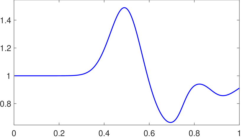
(a) $\eta$ for $t=0.1$

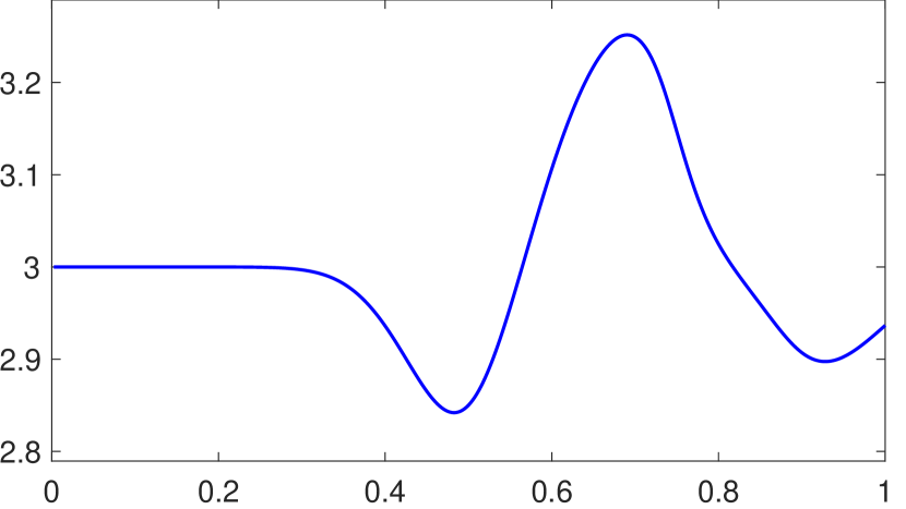
(b) $u$ for $t=0.1$

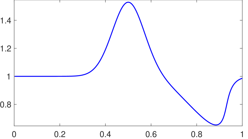
(c) $\eta$ for $t=0.2$

(d) $u$ for $t=0.2$

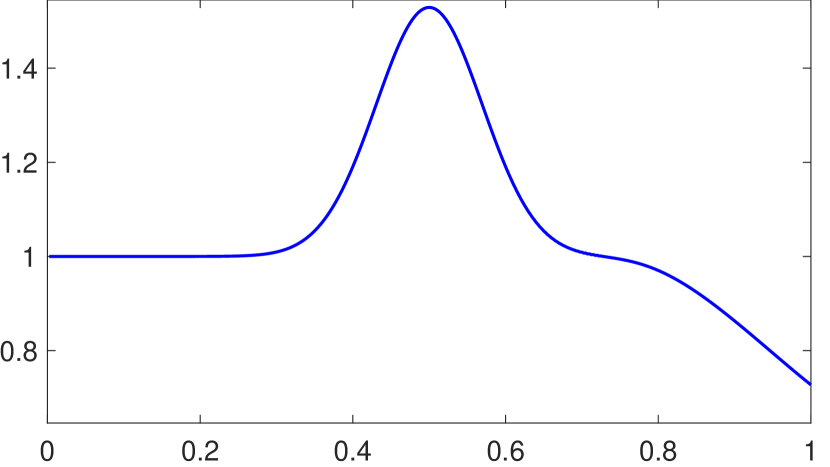
(e) $\eta$ for $t=0.3$

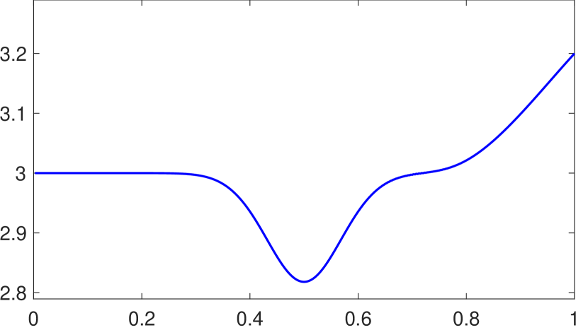
(f) $u$ for $t=0.3$

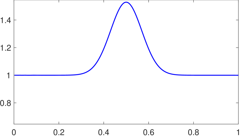
(g) $\eta$ for $t=0.5$

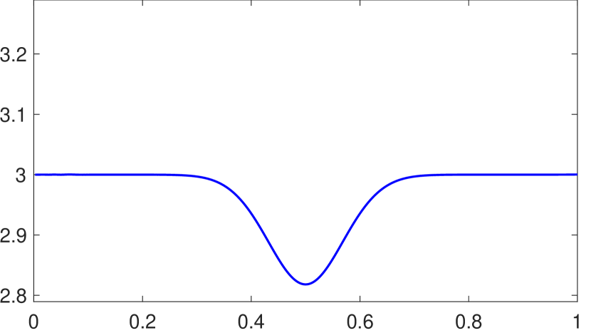
(h) $u$ for $t=0.5$

Figure 1: Evolution with data (3.3), supercritical case, $r=2$, $h=1/400$, $k=h/3$

The steady state of such flows is straightforward to determine analytically. Its profile $\eta=\eta(x)$, $u=u(x)$ satisfies the equations

$$\left((\beta+\eta)u\right)_{x}=0,$$ (3.4)

$$\left(\eta+\tfrac{1}{2}u^{2}\right)_{x}=0,$$

from which using the boundary conditions at $x=0$, we see that $u$ is given in terms of $\eta$ by

$$u=\frac{u_{0}\left(\eta_{0}+\beta(0)\right)}{\eta+\beta},$$ (3.5a)

where $$\eta$$ is the physically acceptable solution of the cubic equation

$$(\eta+\beta)^{2}\left(\eta-\eta_{0}-\tfrac{1}{2}u_{0}^{2}\right)+\tfrac{1}{2}u_{0}^{2}\left(\eta_{0}+\beta(0)\right)^{2}=0.$$ (3.5b)

(For the analysis of the solutions of the steady-state problem, cf. [16]). We checked the ability of the code to preserve steady-state solutions by taking the profile computed analytically from (3.5) for this problem as initial condition and integrating up to $t=0.6$. The difference between the final profile and the $L^{2}$ projection of the analytical initial condition was of $\mathcal{O}(10^{-9})$ in $L^{2}$ for both components when $h=1/400$, $k=h/10$.

In Figure 2 we show instances of the temporal evolution up to the attainment of steady state (in (2(g))) of the supercritical flow generated with $h=1/400$, $k=h/3$, by $\eta_{0}=1$, $u_{0}=3$ and bottom topography and initial conditions given on $[0,1]$ by

$$\beta(x)=1-0.04\exp(-1000(x-0.75)^{2}),$$ (3.6)

$$\eta^{0}(x)=0.05\exp(-400(x-0.25)^{2})+\eta_{0},$$

$$u^{0}(x)=0.1\exp(-400(x-0.25)^{2})+u_{0}.$$

The variable initial profile gives rise to a wavetrain that moves to the right, interacts with the bottom and exits without spurious oscillations leaving behind the steady state that depends only on $\eta_{0}$, $u_{0}$ and $\beta$.

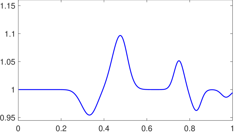
(a) $\eta$ for $t=0.5000$

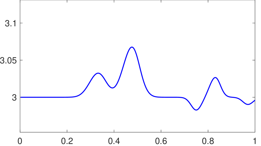
(b) $u$ for $t=0.5000$

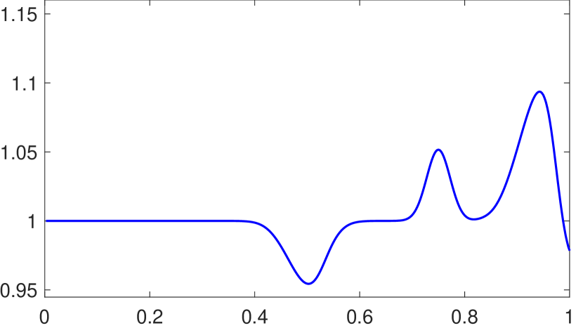
(c) $\eta$ for $t=0.1542$

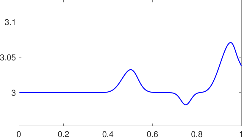
(d) $u$ for $t=0.1542$

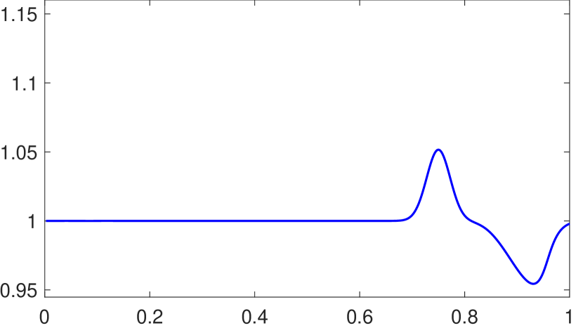
(e) $\eta$ for $t=0.4167$

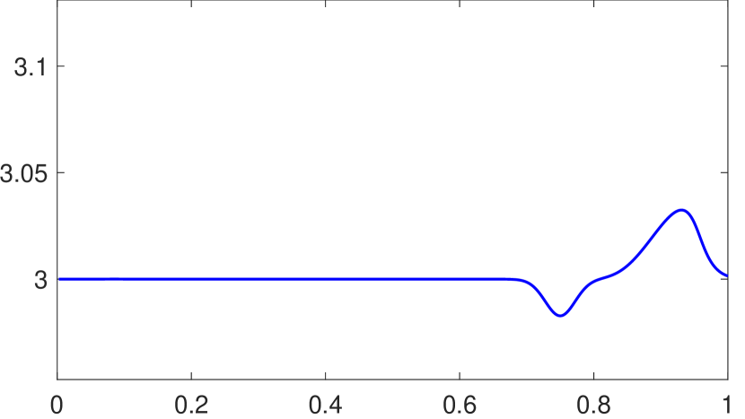
(f) $u$ for $t=0.4167$

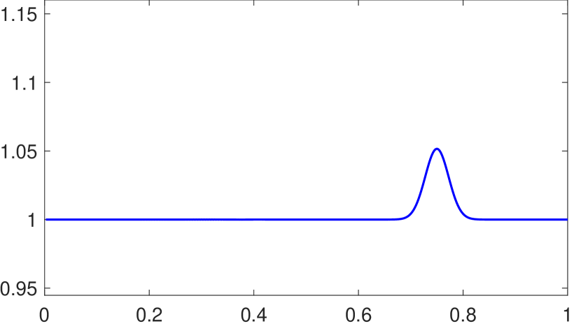
(g) $\eta$ for $t=0.6000$

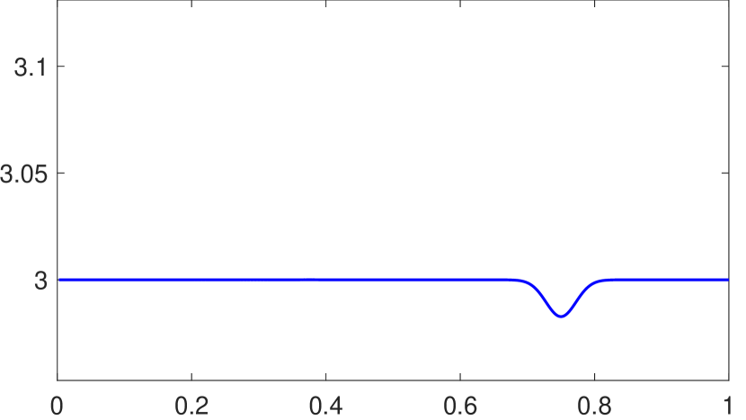
(h) $u$ for $t=0.6000$

Figure 2: Evolution with data (3.6), supercritical case, $r=2$, $h=1/400$, $k=h/3$

We now present some analogous results in the subcritical case . We used the fully discrete scheme with spatial discretization given by (2.50)–(2.52), (2.54); the variables depicted in the figures are the approximations of $\eta$ and $u$. The spatial discretization was effected on $[0,1]$ with piecewise linear functions on a uniform mesh with $h=1/2000$; the time-stepping procedure was RK4 as usual with $k=h/10$. In the first example we took $\eta_{0}=1$, $u_{0}=1$ and

$$\beta(x)=1-0.04\exp(-100(x-0.5)^{2}),$$ (3.7)

$$\eta^{0}(x)=\eta_{0},\quad u^{0}(x)=u_{0}.$$

The ensuing evolution of the solution is shown in Figure 3. The generated wave interacts with the bottom and forms pulses that exit without artificial oscillations at both ends of the boundary; the steady-state solution may be found analytically as before. When used as initial condition, its $L^{2}$ projection differed from the numerical solution at $t=2$ by an $L^{2}$-error of $\mathcal{O}(10^{-8})$ for this example.

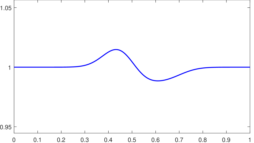
(a) $\eta$ for $t=0.06$

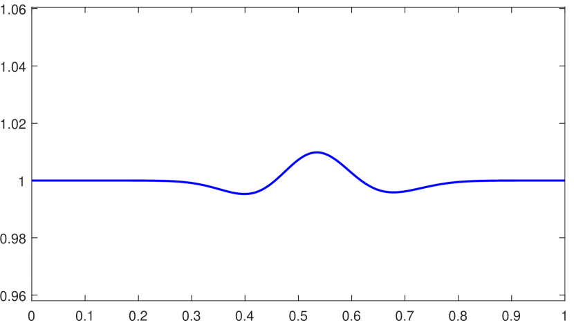
(b) $u$ for $t=0.06$

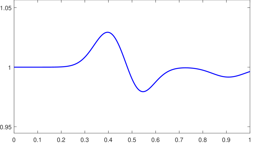
(c) $\eta$ for $t=0.17$

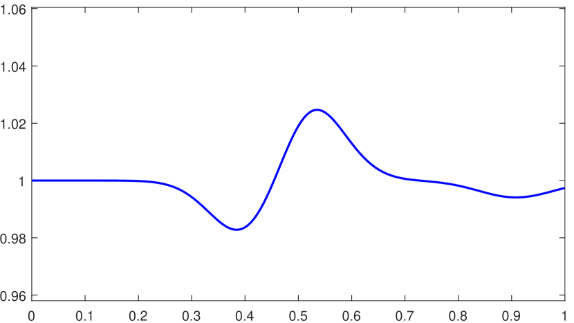
(d) $u$ for $t=0.17$

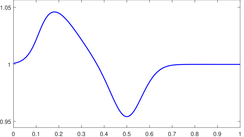
(e) $\eta$ for $t=0.72$

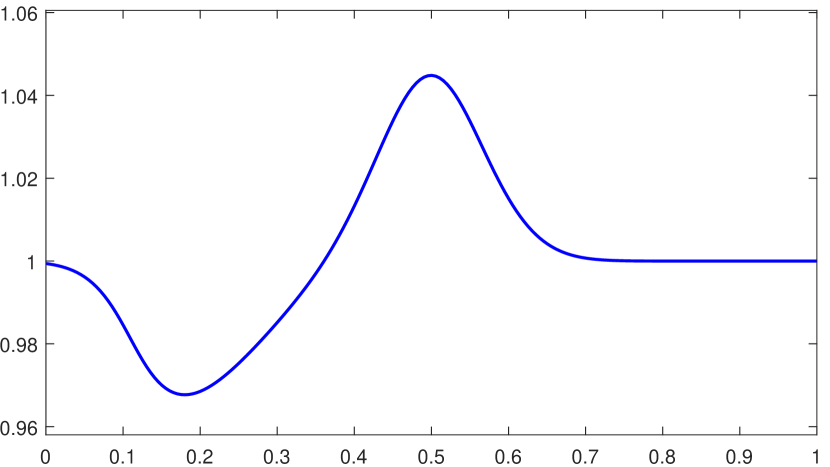
(f) $u$ for $t=0.72$

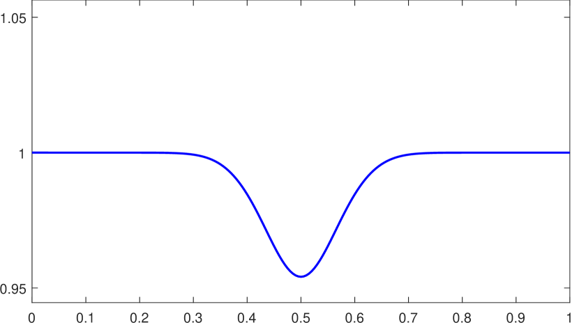
(g) $\eta$ for $t=2$

(h) $u$ for $t=2$

Figure 3: Evolution with data (3.7), subcritical case, $r=2$, $h=1/2000$, $k=h/10$

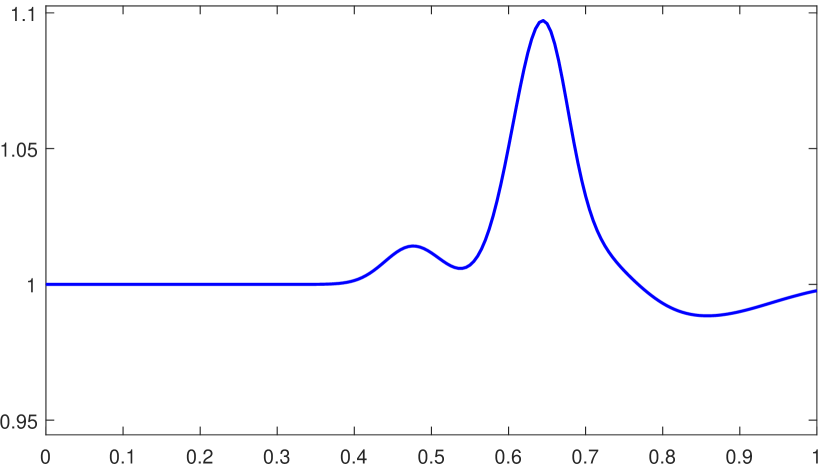
(a) $\eta$ for $t=0.057$

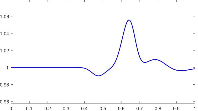
(b) $u$ for $t=0.057$

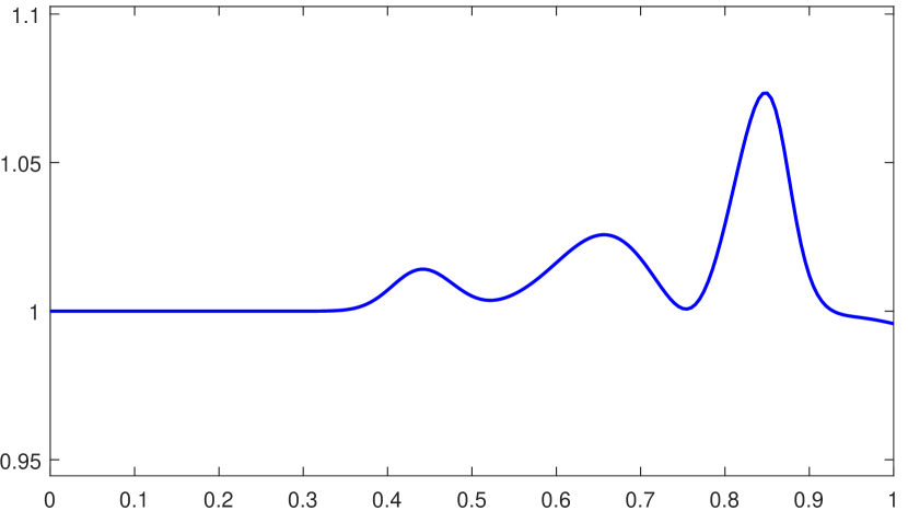
(c) $\eta$ for $t=0.138$

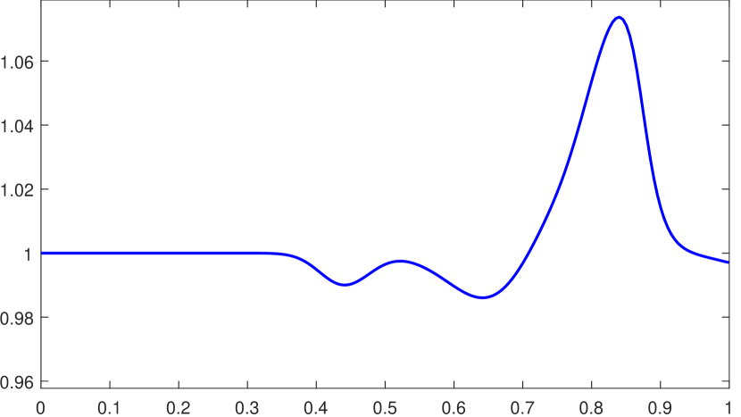
(d) $u$ for $t=0.138$

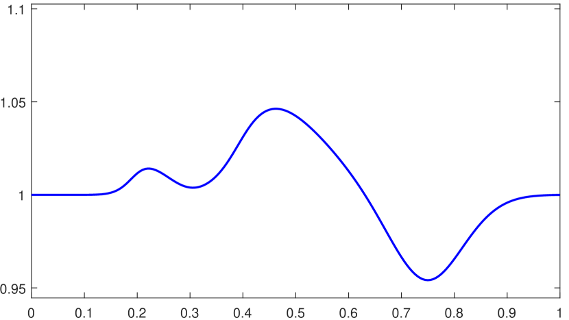
(e) $\eta$ for $t=0.651$

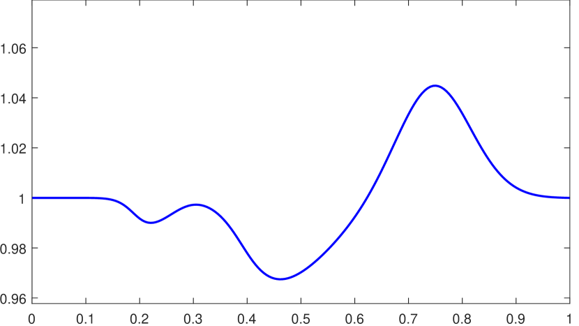
(f) $u$ for $t=0.651$

(g) $\eta$ for $t=3$ (steady state)

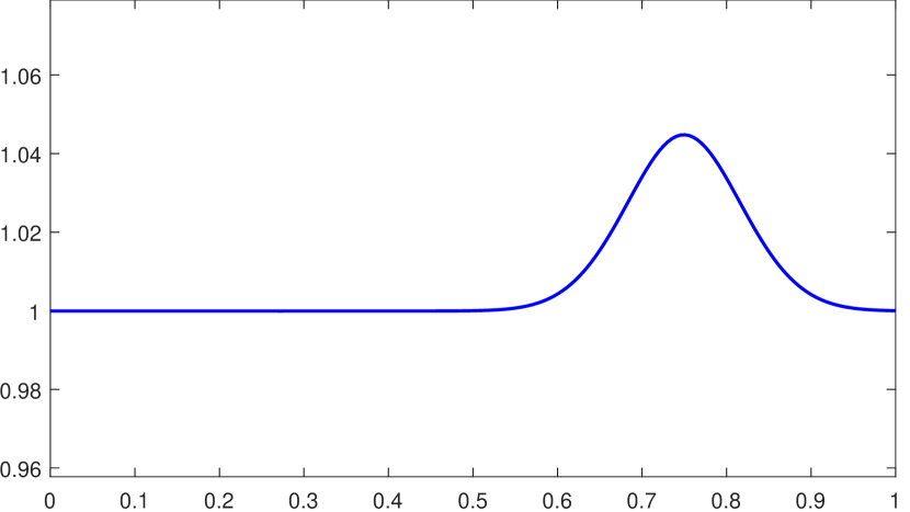
(h) $u$ for $t=3$ (steady state)

Figure 4: Evolution with data (3.8), subcritical case, $r=2$, $h=1/2000$, $k=h/10$

An example of subcritical flow with variable initial conditions is shown in Figure 4, where we took $\eta_{0}=u_{0}=1$, and

$$\beta(x)=1-0.04\exp(-100(x-0.75)^{2}),$$ (3.8)

$$\eta^{0}(x)=0.05\exp(-400(x-0.5)^{2})+\eta_{0},$$

$$u^{0}(x)=0.1\exp(-400(x-0.5)^{2})+u_{0}$$

and integrated with $h=1/2000$, $k=h/10$. A two-way wavetrain emerges and attains steady-state by $t=3$.

We also tested the code in a few examples of the shallow water equations with absorbing (characteristic) boundary conditions, written in dimensional form, i.e. as

$$\begin{aligned} &\eta_{t}+\left((\beta+\eta)u\right)_{x}=0,\\ &u_{t}+g\eta_{x}+uu_{x}=0,\end{aligned}\quad 0\leq x\leq L,\ \ 0\leq t\leq T,$$ (3.9)

with initial conditions $\eta(x,0)=\eta^{0}(x)$, $u(x,0)=u^{0}(x)$, $0\leq x\leq L$, and analogous characteristic boundary conditions in the super- and subcritical cases. (The Riemann invariants are now $u\pm\sqrt{g(\beta+\eta)}$, $g$ is the acceleration of gravity taken as $9.812\,\mathrm{m}/\mathrm{s}^{2}$, and the bottom is at $z=-\beta(x)$. If the bottom is horizontal it is located at $z=-h_{0}$; in the general case $h_{0}$ will be a typical depth.)

As an example of supercritical flow we considered a numerical experiment similar to the one described in Section 8.2 of [5]. Let $\widetilde{\beta}$ be the trapezoidal profile given by

$$\widetilde{\beta}(x)=\begin{cases}\displaystyle\frac{\delta_{0}}{c\kappa-\kappa/2}\left(x-\frac{L}{2}+c\kappa\right),&\text{if}\ \ -c\kappa\leq x-L/2\leq-\kappa/2,\\ \displaystyle\delta_{0},&\text{if}\ \ -\kappa/2\leq x-L/2\leq\kappa/2,\\ \displaystyle-\frac{\delta_{0}}{c\kappa-\kappa/2}\left(x-\frac{L}{2}-c\kappa\right),&\text{if}\qquad\kappa/2\leq x-L/2\leq c\kappa,\\ \displaystyle 0,&\text{otherwise},\end{cases}$$ (3.10)

where $L=10^{6}\,\mathrm{m}$, $\delta_{0}=500\,\mathrm{m}$, $k=L/10$. The bottom was located at $z=-\beta(x)$, where $\beta(x)=h_{0}-\widetilde{\beta}(x)$, $h_{0}=1000\,\mathrm{m}$, and the problem (3.9) was solved with characteristic boundary conditions and initial conditions $\eta^{0}(x)=\eta_{0}=0$ and $u^{0}(x)=u_{0}$, where the constant $u_{0}$ was varied in order to give flows with different Froude numbers $Fr=u_{0}/\sqrt{gh_{0}}$. We solved (3.9)–(3.10) numerically with piecewise linear elements and RK4 on a uniform mesh with $h=1000\,\mathrm{m}$, $k=1\,\mathrm{s}$. Some profiles of the steady state of the free surface $\eta$ and the associated bottom function $\beta(x)$ for various Froude numbers and values of the parameter $c$ are shown in Figure 5. As expected the eventual maximum value of $\eta$ decreases as $Fr$ increases; the results are consistent with those of [5].

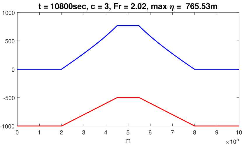
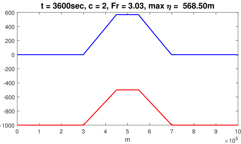
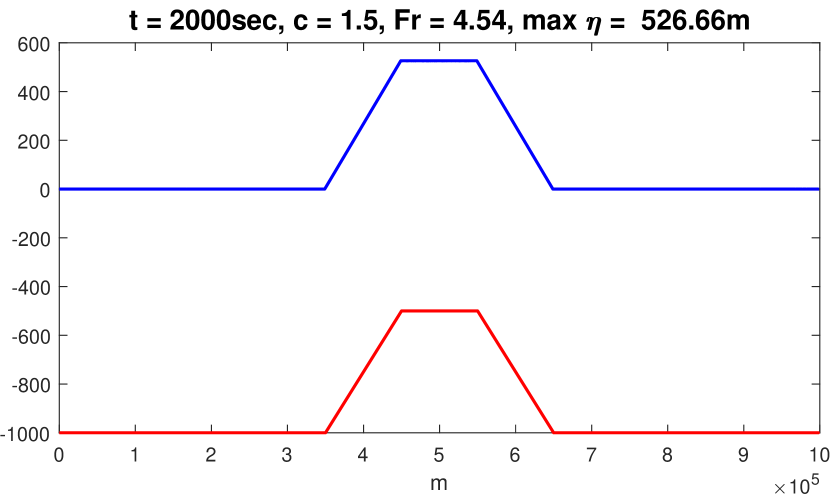
Figure 5: Supercritical flows over a trapezoidal bottom, (3.9)–(3.10), $r=2$, $h=1000\,\mathrm{m}$, $k=1\,\mathrm{s}$. (Upper figures: steady-state $\eta(x)$; lower figures: $\beta(x)$.)

In an example of a dimensional subcritical flow we modified the profile given in §5.1 of [5] in order to avoid discontinuity formation. Thus, the initial $\eta$-profile was rounded and its amplitude decreased. Let $\widetilde{\beta}$ be defined by

$$\widetilde{\beta}(x)=\begin{cases}\displaystyle\frac{\delta}{2}+\frac{\delta}{2}\cos\left[\frac{\pi(x-L/2)}{\kappa}\right],&\displaystyle\text{if}\ \ \left|x-\frac{L}{2}\right|<\kappa,\\ 0,&\text{otherwise},\end{cases}$$ (3.11)

where $L=10^{6}\,\mathrm{m}$, $\delta=5000\,\mathrm{m}$, $k=L/10$. The bottom was taken at $z=-\beta(x)$, where $\beta(x)=h_{0}-\widetilde{\beta}(x)$, $h_{0}=10^{4}\,\mathrm{m}$, and the problem (3.9) was solved with characteristic boundary conditions with $\eta_{0}=u_{0}=0$ and $\eta^{0}(x)=0.2\,\varepsilon\,h_{0}\exp\left[-5{\cdot}10^{-8}\left(x-3L/20)/10\right)^{2}\right]$, $0\leq x\leq L$, where $\varepsilon=0.2$.

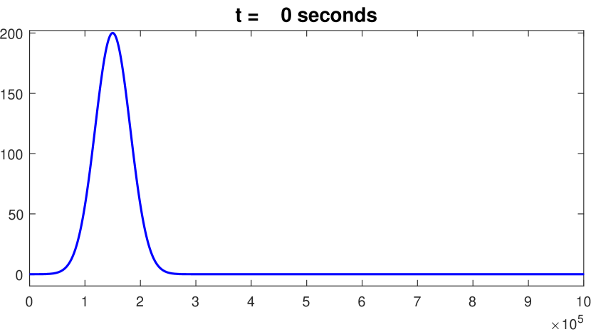
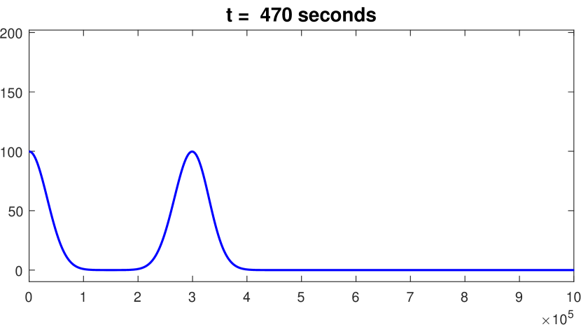
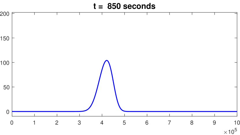
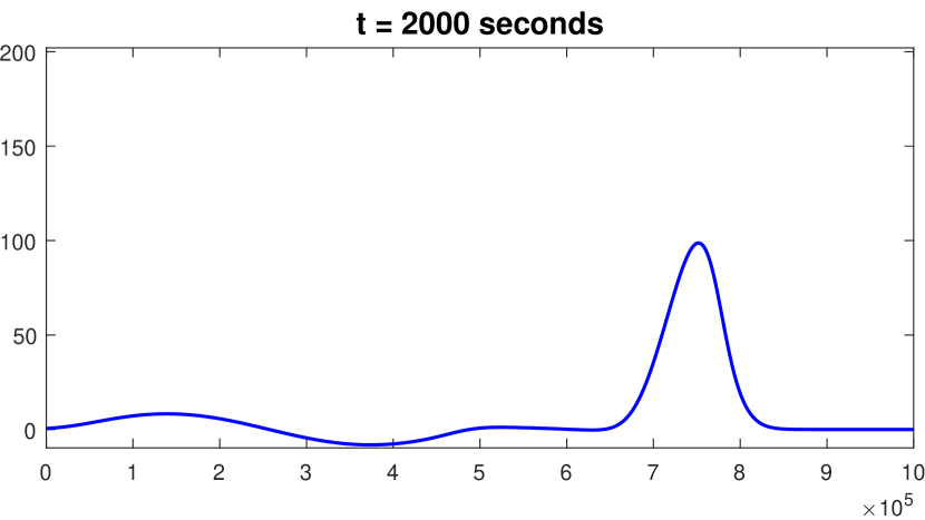
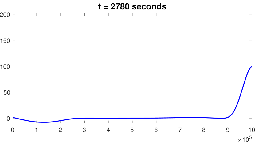
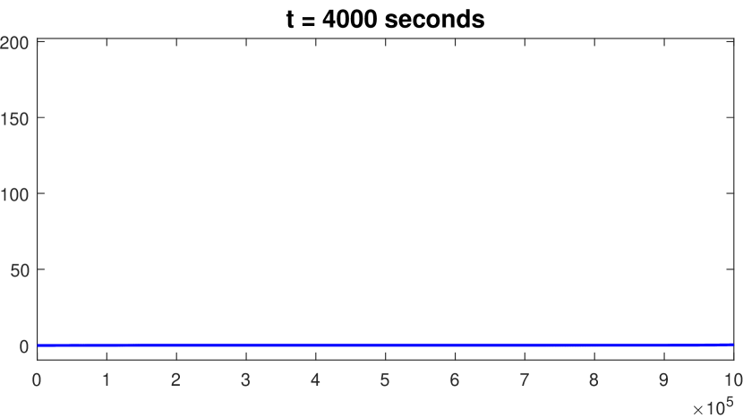
Figure 6: Subcritical flow over a hump, (3.9), (3.11), $r=2$, $h=1000\,\mathrm{m}$, $k=1\,\mathrm{s}$, $\eta$ profiles

The evolution of the $\eta$-profiles is shown in Figure 6 up to the attainment of the steady state $\eta=u=0$. The results resemble qualitatively those of [5].

3.2 Shallow water equations in balance-law form

In this section we consider the numerical solution by the standard Galerkin finite element method of the shallow water equations written in balance-law form (i.e. in conservation-law form with a source term), as

$$d_{t}+(du)_{x}=0,$$ (3.12)

$$(du)_{t}+\left(du^{2}+\tfrac{1}{2}d^{2}\right)_{x}=\beta^{\prime}(x)d,$$

where $d=\eta+\beta$ is the water depth assumed as always to be positive; the variables in (3.12) are nondimensional. Is is straightforward to see that the system (3.12) is equivalent to (SW) since $d\neq 0$. In the sequel we will consider the periodic initial-value problem for (3.12) on the spatial interval $[0,1]$ and assume that it has sufficiently smooth solutions for $t\in[0,T]$, provided that $\beta$ is smooth and $1$-periodic. We will discretize the problem in space on a uniform or quasiuniform mesh $\{x_{i}\}$ in $[0,1]$ and seek approximations $d_{h}$, $u_{h}$ of $d$, $u$, respectively, in the finite element space $S_{h,p}=\{\phi\in C_{p}^{k}:\phi\big{|}_{[x_{j},x_{j+1}]}\in\mathbb{P}_{r-1},\text{all}\ j\}$, where as usual $r$, $k$ are integers such that $r\geq 2$, $0\leq k\leq r-2$, and $C_{p}^{k}$ are the $k$ times continuously differentiable, periodic functions on $[0,1]$. The semidiscrete approximations satisfy

$$\begin{aligned} &(d_{ht},\phi)+((d_{h}u_{h},\phi)=0,\\ &((d_{h}u_{h})_{t},\phi)+((d_{h}u_{h}^{2}+\tfrac{1}{2}d_{h}^{2})_{x},\phi)=(\beta^{\prime}d_{h},\phi),\end{aligned}\ \ \forall\phi\in S_{h,p},\ 0\leq t\leq T,$$ (3.13)

$$d_{h}(0)=\operatorname{P}d^{0},\quad u_{h}(0)=\operatorname{P}u^{0},$$ (3.14)

where $d^{0}$, $u^{0}$ are the initial conditions of $d$ and $u$ and $\operatorname{P}$ is now the $L^{2}$ projection operator onto $S_{h,p}$. (The second equation in (3.13) is advanced in time for the variable $v_{h}=d_{h}u_{h}$ and $u_{h}$ is recovered as $v_{h}/d_{h}$.) In the case of a uniform mesh it is expected that the $L^{2}$ errors of the semidiscrete solution will be of $\mathcal{O}(h^{r})$ while, for a quasiuniform mesh, of $\mathcal{O}(h^{r-1})$, cf. [10]. We verified these rates of accuracy in numerical experiments using $C^{0}$ linear, $C^{2}$ cubic and $C^{4}$ quintic splines (i.e. spaces $S_{h,p}$ with $r=2$, $4$, and $6$, respectively) on uniform and nonuniform spatial meshes, coupled with explicit Runge Kutta schemes of third, fourth, and sixth order of accuracy, respectively. The fully discrete methods were stable under Courant number restrictions. We note that in order to preserve the optimal order of accuracy, say in the case of a uniform mesh, one has to compute the integrals that occur in the finite element equations using, on each subinterval $[x_{i},x_{i+1}]$, an $s$-point Gauss quadrature rule with $s\geq r-1$. For example, in the case of a cubic spline spatial discretization, a 3-point Gauss rule is sufficient.

It is interesting to examine whether the method (3.13)–(3.14) preserves the still water solution $\eta=0$, $u=0$, e.g. of the periodic i.v.p. for the shallow water equations in the form (3.12). Discretizations that approximate accurately this solution are called ‘well balanced’, cf. e.g. [13], and [7] and its references. (It is easy to check that the standard Galerkin semidiscretization of e.g. the periodic ivp for (SW), i.e. for the shallow water equations in their ‘nonconservative’ form, is trivially well-balanced, since it satisfies $\eta_{h}(x,t)=\alpha$, $\alpha$ constant, $u_{h}(x,t)=0$ for all $t\geq 0$ and $x\in[0,1]$, provided $\eta_{h}(x,0)=\alpha$, $u_{h}(x,0)=0$. So, our attention is turned to the periodic ivp for (3.12) and its standard Galerkin semidiscretization (3.13)–(3.14).)

For this purpose, since $d=\eta+\beta$, assume that (suppressing the $x$-dependence in the variables), $d_{h}(0)=\operatorname{P}\beta$, $u_{h}(0)=0$ in (3.14), and ask whether there exist time-independent solutions of (3.13)–(3.14) that approximate well the steady state solution $d=\beta$, $u=0$ of the continuous problem. Taking $u_{h}=0$ in (3.13) we see that a steady-state solution $d_{h}$ must satisfy $(d_{h}d_{hx},\phi)=(d_{h}\beta^{\prime},\phi)$, for all $\phi$ in $S_{h,p}$, from which it is evident that the source term $\beta$ should be replaced by some approximations $\beta_{h}\in S_{h,p}$ thereof. Moreover for the equation $(d_{h}d_{h,x},\phi)=(d_{h}\beta_{h}^{\prime},\phi)$ to hold for $\phi\in S_{h,p}$, (this will imply that $d_{h}=\beta_{h}$, i.e. good balance), it is necessary that the integrals on each subinterval $[x_{i},x_{i+1}]$ that contribute to these $L^{2}$ inner products should be evaluated exactly. Since both integrands are polynomials of degree at most $3r-4$ on each subinterval, if an $s$-point Gauss quadrature rule is used (recall that such a rule is exact for polynomials of degree at most $2s-1$), then it should hold that $s\geq\tfrac{3}{2}(r-1)$. For example, in the case of cubic splines $(r=4)$, a 5-point Gauss rule must be used. Therefore, although a 3-point Gauss is enough to preserve the optimal-order $\mathcal{O}(h^{4})$ $L^{2}$-error estimate, good balance of the solution with cubic splines requires that a 5-point Gauss rule be used. This is confirmed by the results of the following experiment. We solve the periodic ivp for (3.12) on $[0,1]$ by (3.13)–(3.14) using cubic splines for the spatial discretization on a uniform mesh and taking $\beta(x)=1-0.3\exp(-1000(x-0.5)^{2})$, $h=0.02$, $k=0.01$, $u_{h}(0)=0$, $d_{h}(0)=\operatorname{P}\beta$. Table 3 shows the error $d_{h}(1)-d_{h}(0)$ (where $d_{h}(1)=d_{h}\big{|}_{T=1}$) in the $L^{2}$ and $L^{\infty}$ norms when the analytical formula of $\beta$ or $\beta_{h}=\operatorname{P}\beta$ is taken in the source term, and a 3- or a 5-point Gauss rule is used. It is evident that when $b_{h}=\operatorname{P}\beta$ and

$d_{h}(0)$	$\beta$ in source term	$s$ (-point Gauss rule)	$\|d_{h}(1)-d_{h}(0)\|$	$\|d_{h}(1)-d_{h}(0)\|_{\infty}$
$\operatorname{P}\beta$	analytical formula	3	1.8191e-40	8.3845e-40
$\operatorname{P}\beta$	$\beta_{h}=\operatorname{P}\beta$	3	1.2204e-60	4.7085e-60
$\operatorname{P}\beta$	$\beta_{h}=\operatorname{P}\beta$	5	3.7458e-15	1.0214e-14

Table 3: Treatment of source terms and effect of quadrature in (3.13)--(3.14), cubic splines and RK4, $h=0.02$, $k=0.01$, $T=1$

a 5-point Gauss quadrature rule is used, the scheme is well balanced to roundoff and there is no influence of the time-stepping error. It should be noted that similar results were found when $d_{h}(0)$ and $\beta_{h}$ were taken as the cubic spline interpolant of $\beta$ at the nodes, and when piecewise smooth bottom profiles, e.g. like a parabolic perturbation of $\beta=1$ supported in the interval of $[0,1]$, were considered.

References

- [1] D. H. Peregrine, Equations for water waves and the approximation behind them, in: R. Meyer (Ed.), Waves on Beaches and Resulting Sediment Transport, Academic Press, New York, 1972, pp. 95–121.
- [2] M. Petcu, R. Temam, The one dimensional Shallow Water equations with Dirichlet boundary conditions on the velocity, Discrete Contin. Dyn. Syst. Ser. S 4 (1) (2011) 209–222.
- [3] A. Huang, M. Petcu, R. Temam, The one-dimensional supercritical shallow-water equations with topography, Annals of the University of Bucharest (Mathematical Series) 2 (LX) (2011) 63–82.
- [4] M. Petcu, R. Temam, The one-dimensional shallow water equations with transparent boundary conditions, Mathematical Methods in the Applied Sciences 36 (15) (2013) 1979–1994.
- [5] M.-C. Shiue, J. Laminie, R. Temam, J. Tribbia, Boundary value problems for the shallow water equations with topography, J. Geophys. Res. 116 (C02015) (2011) 1–22. doi:10.1029/2010JC006315.
- [6] J. Nycander, A. M. Hogg, L. M. Frankcombe, Open boundary conditions for nonlinear channel flow, Ocean Modelling 24 (3-4) (2008) 108–121.
- [7] Y. Xing, X. Zhang, C.-W. Shu, Positivity-preserving high order well-balanced discontinuous Galerkin methods for the shallow water equations, Advances in Water Resources 33 (12) (2010) 1476–1493.
- [8] J. Qiu, Q. Zhang, Stability, error estimate and limiters of discontinuous Galerkin methods, in: R. Abgrall, C.-W. Shu (Eds.), Handbook of Numerical Analysis, Vol. 17, Elsevier, 2016, pp. 147–171.
- [9] Y. Xing, Numerical Methods for the Nonlinear Shallow Water Equations, in: R. Abgrall, C.-W. Shu (Eds.), Handbook of Numerical Analysis, Vol. 18, Elsevier, 2017, pp. 361–384.
- [10] D. Antonopoulos, V. Dougalis, Error estimates for the standard Galerkin-finite element method for the shallow water equations, Mathematics of Computation 85 (299) (2016) 1143–1182.
- [11] D. Antonopoulos, V. Dougalis, Galerkin-finite element methods for the shallow water equations with characteristic boundary conditions, IMA Journal of Numerical Analysis 37 (1) (2017) 266–295.
- [12] D. Antonopoulos, V. Dougalis, G. Kounadis, On the standard Galerkin method with explicit RK4 time stepping for the Shallow Water equations, arXiv preprint arXiv:1810.11008.
- [13] A. Bermudez, M. E. Vázquez, Upwind methods for hyperbolic conservation laws with source terms, Computers & Fluids 23 (8) (1994) 1049–1071.
- [14] J. Douglas, T. Dupont, L. Wahlbin, Optimal error estimates for Galerkin approximations to solutions of two-point boundary value problems, Mathematics of Computation 29 (130) (1975) 475–483.
- [15] T. Dupont, Galerkin methods for first order hyperbolics: an example, SIAM Journal on Numerical Analysis 10 (5) (1973) 890–899.
- [16] D. D. Houghton, A. Kasahara, Nonlinear shallow fluid flow over an isolated ridge, Communications on Pure and Applied Mathematics 21 (1) (1968) 1–23.