First-principles calculations of the magnetocrystalline anisotropy of the prototype 2:17 cell boundary phase Y(Co_1-x-yFe_xCu_y)₅

Abstract

We present a computational study of the compound Y(Co_1-x-yFe_xCu_y)₅ for 0 $\leq x,y\leq 0.2$. This compound was chosen as a prototype for investigating the cell boundary phase believed to play a key role in establishing the high coercivity of commercial Sm-Co 2:17 magnets. Using density-functional theory, we have calculated the magnetization and magnetocrystalline anisotropy at zero temperature for a range of compositions, modeling the doped compounds within the coherent potential approximation. We have also performed finite temperature calculations for YCo₅, Y(Co_0.838Cu_0.162)₅ and Y(Co_0.838Fe_0.081Cu_0.081)₅ within the disordered local moment picture. Our calculations find that substituting Co with small amounts of either Fe or Cu boosts the magnetocrystalline anisotropy $K$, but the change in $K$ depends strongly on the location of the dopants. Furthermore, the calculations do not show a particularly large difference between the magnetic properties of Cu-rich Y(Co_0.838Cu_0.162)₅ and equal Fe-Cu Y(Co_0.838Fe_0.081Cu_0.081)₅, despite these two compositions showing different coercivity behavior when found in the cell boundary phase of 2:17 magnets. Our study lays the groundwork for studying the rare earth contribution to the anisotropy of Sm(Co_1-x-yFe_xCu_y)₅, and also shows how a small amount of transition metal substitution can boost the anisotropy field of YCo₅.

1 Introduction

Of the wide variety of magnetic materials that can be formed by alloying rare-earth elements with transition metals (RE/TM) [1], the permanent magnet market is dominated by those based either on Nd-Fe-B [2, 3] or Sm-Co [4, 5]. The performance of a permanent magnet is usually quantified by its maximum energy product $(BH)_{\mathrm{max}}$, which measures the energy stored in the air gap of the associated magnetic circuit [6]. At temperatures up to approximately 120^∘C, the Nd-Fe-B materials have the highest $(BH)_{\mathrm{max}}$ of all available permanent magnetic materials, but above this temperature their excellent performance sharply diminishes [7]. By contrast, Sm-Co magnets do not have the same dramatic sensitivity to temperature as Nd-Fe-B, showing superior performance above 120^∘C [7] and even operating at temperatures in excess of 400^∘C [8]. Sm-Co magnets are therefore the materials of choice for applications where high-temperature performance is critical, e.g. sensing in manufacturing processes [9].

The Sm-Co magnets can be further partitioned into the 1:5 and 2:17 classes based on their nominal crystal structures, with the highest-performing magnets falling into the 2:17 class [10]. As well as Sm and Co, commercial 2:17 magnets also contain Fe, Cu and Zr at an approximate stoichiometry Sm(Co_1-x-y-uFe_xCu_yZr_u)_z, where $z\sim 7.5$, $x,y\sim 0.1$ and $u\sim 0.01$ [11]. As illustrated by the value of $z$, the 2:17 magnets also do not simply consist of a single Sm₂TM₁₇ phase but rather adopt a multi-phase structure [12]. This structure consists of a cellular phase composed of 2:17 cells surrounded by thin ($\sim$10 nm) cell boundaries with an approximate 1:5 stoichiometry, and a lamellar, Zr-rich “Z” phase [13].

It has long been accepted that this complex multi-phase structure is essential to maintaining the excellent high-temperature performance of the 2:17 magnets [10]. Recent work has highlighted the importance of the Z phase in aiding the formation of the cellular phase [14]. The critical role played by the cellular phase is then revealed by electron microscopy experiments, which show the pinning of magnetic domain walls at 2:17/1:5 boundaries [15]. This domain wall pinning inhibits magnetization reversal and thus provides a coercive force.

Over the years a number of theories have been proposed to explain the pinning of the domain walls [15, 16, 17, 18, 19, 20, 21, 22, 23, 24, 25]. According to micromagnetic theory [26], the energy of a domain wall depends both on the strength of the exchange interaction $A$ and the magnetic anisotropy $K$ as $\propto\sqrt{AK}$. Assuming that the 2:17 cells and 1:5 cell boundary phases have different $A$ and $K$, there will be an energy barrier associated with a domain wall moving between these regions [16]. Interestingly, this argument does not rely on the domain wall energy being larger or smaller in the cell boundary phase compared to the cell [17]. In models based on “repulsive” pinning, the domain wall energy is higher in the cell boundary phase, so the domain wall gets stuck in the cell [18, 16, 19], while in “attractive” pinning models the domain walls have higher energies in the cell, so they get pinned in the cell boundary phase instead [20, 15, 21, 22]. More recently, models have been proposed where it is the variation of $K$ within the cell boundary region that determines the coercivity [23, 24, 25].

The existence of different models reflect the complicated nature both of 2:17 magnets and of coercivity in general. Indeed, the small size of the cell boundary phase and of the domain walls themselves already presents a challenge to continuum-based micromagnetics [20]. However, assuming micromagnetics can be used to gain insight into the magnetization reversal process, a basic question is what values of $A$, $K$ and magnetic polarization $J$ should be used as input in the simulations. Focusing on the magnetic anisotropy $K$, based upon the values measured for SmCo₅ and Sm₂Co₁₇ one would expect a much larger anisotropy in the 1:5 cell boundary phase compared to the 2:17 cells. Indeed, there are reports of measurements on a commercial 2:17 sample which support this view [16]. However, other experimental studies concluded that the 1:5 cell boundary was actually softer (smaller anisotropy) than the cell [21]. Another study found similar anisotropy energies for the two phases, but explained the pinning of domain walls in terms of a large difference in exchange energy $A$ between the phases [20].

Of course, a crucial property of the commercial magnets is the presence of the additional elements Cu, Fe and Zr. A recent 3D atom probe study measured the chemical compositions of the cell boundary phase for 2:17 magnets showing both high and low coercivities, depending on heat treatment [25]. This study reported that the high-coercivity sample coincided with an enhanced Cu and diminished Fe content in the 1:5 cell boundary, as well as a sharp interface between the cell and cell boundary phases. Conversely, having a similar Fe and Cu content in the 1:5 cell boundary, as well as having a diffusive interface between the cell and cell boundary phases, was correlated with low coercivity [25]. The Zr content was found to be very small in both cases.

It would be desirable to be able to establish a link between chemical composition and magnetic properties. In Ref. [25] it is pointed out that, although there is some data on binary Sm(Co,Cu)₅ (e.g. Ref. [27]), there is a gap in the literature considering the ternary compound Sm(Co_1-x-yFe_xCu_y)₅. Indeed we note that even the experimental data of Ref. [27] on Sm(Co_1-yCu_y)₅ only reports anisotropy fields measured for $y\geq 0.24$ ($\geq$20% by atom) which is already larger than the $\sim$15% measured in the cell boundary phase in Ref. [25]. The modification of TM content by the substitution of Co with Cu and Fe can be expected to change the magnetic anisotropy of SmTM₅ in a number of ways, namely: (a) affecting the single ion anisotropy of Sm by modifying the crystal field [28] (b) affecting the temperature dependence of this single ion anisotropy by modifying the exchange field felt by the RE due to the RE/TM interaction [29] and (c) modifying the contribution of the TM-3$d$ electrons to the anisotropy[30, 31, 32, 33, 34]. The introduction of Fe and Cu can also be expected to affect the other key micromagnetic parameters $A$ and polarization $J$, leading for example to modified Curie temperatures [35]. Furthermore, changing the local environment of the Sm atoms may even modify their valency and orbital hybridization, further affecting the anisotropy [36].

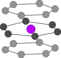
Figure 1: Schematic representation of RETM₅ crystal structure (space group 191, $P6/mmm)$, showing the RE site (purple) and two inequivalent TM sites: the $2c$ position (in plane with RE, dark grey), and the $3g$ position (out of plane, light grey).

As a first step towards obtaining an improved understanding of how the magnetic properties of the cell boundary phase are affected by chemical composition, we have performed first-principles (density-functional theory) calculations on the ternary compound Y(Co_1-x-yFe_xCu_y)₅ (Fig. 1). The reasons for first investigating Y rather than Sm are twofold: first, although Y has the same $s^{2}d$ valence structure as Sm, the absence of 4$f$ electrons means that we can isolate the Tm-$3d$ contribution to the anisotropy [point (c) above] from the single ion contribution [(a) and (b)]. Second, YCo₅ remains an interesting magnet in its own right, being free of lanthanide elements [37], having an anisotropy field of order 20 T [38] and potentially having a coercivity comparable to traditional SmCo₅ magnets [39]. Indeed, Fe-doped YCo₅ magnets are the subject of active research as potential intermediate-performance permanent magnets [40].

Our study consists of two parts. In the first part, we calculate the zero-temperature properties (magnetization and magnetocrystalline anisotropy) of Y(Co_1-x-yFe_xCu_y)₅ for 0 $\leq x,y\leq 0.2$. The studied compositions fall into the ranges previously investigated in experiments on binary compounds [41, 42]. The chemical disorder is modelled within the coherent potential approximation (CPA) [43]. In the second part, we concentrate on the compounds YCo₅, Y(Co_0.838Cu_0.162)₅ and Y(Co_0.838Fe_0.081Cu_0.081)₅ and calculate their finite temperature properties within the disordered local moment (DLM) picture [44]. These particular concentrations were chosen based on the experimentally-measured compositions of the cell boundary phases of (Sm-Co) 2:17 magnets which showed high and low coercivity respectively in Ref. [25].

The current manuscript aims to address the gap in the literature concerning the intrinsic properties of the ternary Y(Co_1-x-yFe_xCu_y)₅ compound. From a technical aspect, due to the current lack of studies which have used the CPA to model the doping, the manuscript includes some technical discussion, such as a comparison of the CPA with the simpler “rigid band” approach. However, we also aim to make a practical connection to Ref. [25] by reporting values of the anisotropy field and micromagnetic parameters $A$, $K$ and $J$ for the representative high and low coercivity cell boundary compositions. We hope that such parameters might be useful for future micromagnetics calculations like those originally performed in Ref. [25]. In this way we follow recent works on RE/TM magnets which have demonstrated how microscopic quantities can be incorporated into large scale simulations [45, 46].

Interestingly, the zero temperature calculations find that a low level of substitution enhances the magnetocrystalline anisotropy, regardless of whether Co is substituted with Fe or Cu. In particular, substituting $\sim$15% of Co yields the largest anisotropy energies. The calculations also demonstrate how the anisotropy is very sensitive to the location of the dopant atoms.

We find that the calculated difference between Cu-rich and equal Cu-Fe substitution is not particularly large. The current calculations therefore do not indicate that the TM-3$d$ contribution to the anisotropy of the cell boundary phase is an important factor in determining the coercivity of the 2:17 magnets. Nonetheless, our study lays the groundwork for studying the RE contribution to the anisotropy of Sm(Co_1-x-yFe_xCu_y)₅, and highlights the route of boosting the anisotropy field of YCo₅ through TM substitution.

Our manuscript is organized as follows. In Section 2 we outline the methods used to calculate magnetic properties at zero and finite temperature. The calculated results are presented in Section 3 and analyzed in Section 4. We present our conclusions and discuss future directions for study in Section 5.

2 Calculation details

All calculations were performed within the multiple-scattering, Korringa-Kohn-Rostocker (KKR) formulation of density-functional theory (DFT) [47], treating exchange and correlation effects within the local spin-density approximation (LSDA) [48]. Scalar-relativistic calculations were performed within the atomic sphere approximation (ASA) for the charge density and potential using the Hutsepot KKR code [49], solving the scattering problem up to a maximum angular momentum quantum number $l_{\mathrm{max}}=3$ and sampling the Brillouin zone on a 20$\times$20$\times$20 grid. The Y-4$p$ electrons were treated explicitly as valence states. The self-consistent potentials were obtained for the T=0 K, ferromagnetic arrangement of magnetic moments.

Substitutional doping of Co with Fe or Cu was modeled within the CPA [43, 47]. For all compositions the lattice parameters were kept fixed to the values $a$,$c$, = 4.950, 3.986 Å, as measured experimentally for YCo₅ at 300 K [50].

To calculate magnetic properties, the “frozen” scalar-relativistic potentials were inserted into the Kohn-Sham-Dirac equation in order to solve the fully-relativistic scattering problem [51]. Spin and orbital magnetic moments were calculated by tracing the appropriate operators with the Green’s function [52]. The magnetocrystalline anisotropy energy was obtained via the torque, i.e. the change in free energy on rotation of the magnetization vector [53, 54]. An adaptive algorithm for the Brillouin zone integration was used to ensure high numerical precision [55].

Finite temperature properties were calculated within the disordered local moment picture, which treats the temperature-induced fluctuations of the local moments at the level of the CPA [44]. The temperature-dependent Weiss fields were determined using an iterative procedure [34, 35]. Both an overview of DFT-DLM and the detailed procedure of evaluating the Weiss fields and torque can be found elsewhere, e.g. Ref. [54].

Previous computational studies on YCo₅ found the LSDA to yield values of both the orbital magnetic moments and the magnetocrystalline anisotropy which are smaller than measured experimentally, but including an orbital polarization correction (OPC) [56] on the TM-$d$ orbitals corrects this discrepancy [30, 31, 32]. Although the relativistic DFT-DLM calculations do allow an OPC to be included [29, 57, 58], in the current work we do not do so due to the large number of (Fe,Cu) compositions considered. Therefore our calculated anisotropy energies are underestimates compared to experiment. Test calculations for selected compositions found the same qualitative trends to be obeyed by OPC and non-OPC calculations, but more work is necessary to perform a full comparison of the two approaches.

3 Results

3.1 Anisotropy at zero temperature: rigid band model

For a crystal with hexagonal symmetry, the expected variation of the free energy with magnetization angle $\theta$ is $K_{1}\sin^{2}\theta+K_{2}\sin^{4}\theta+\mathcal{O}(\sin^{6}\theta)$, where $\theta$ is given with respect to the $c$ axis. Evaluating the torque $\partial F/\partial\theta$ at $\theta=45^{\circ}$ yields $K_{1}+K_{2}$, which we label $K$. Previous experimental and theoretical studies [38, 58] have determined $K_{2}$ to be an order of magnitude smaller than $K_{1}$ in pristine YCo₅, so $K\approx K_{1}$. A positive value of $K$ corresponds to out-of-plane anisotropy.

The most straightforward method of simulating the substitutional doping of Co with Fe or Cu is to use the rigid band approximation, i.e. simply shift the Fermi level in the DFT calculation of pristine YCo₅ so that the total number of electrons in the unit cell matches that expected for the doped system. YCo₄Fe corresponds to a change in electron number of $\Delta N_{e}=-1$, while YCo₄Cu corresponds to $\Delta N_{e}=+2$.

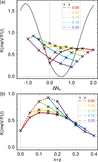
Figure 2: (a) Anisotropy energy $K$ per formula unit (FU) as a function of change in electron number $N_{e}$, calculated for Y(Co_1-x-yFe_xCu_y)₅ either in the rigid band approximation (black dotted line) or with the CPA (crosses). Each cross lies on the intersection of a solid ($x$) and dashed ($y$) line which allows the composition to be deduced. (b) The same CPA calculations as (a) replotted as a function of dopant content $x+y$.

The anisotropy $K$ calculated in this way is shown as the dotted line in Fig. 2(a). As noted in previous works [30, 31, 32, 34] there is a pronounced dependence of $K$ on the band filling. As discussed at length in Ref. [31], the anisotropy energy originates from the splitting of otherwise degenerate states by the spin-orbit interaction, with the strongest contributions coming from states with energies close to the Fermi level. Shifting the Fermi level changes the weights of the contribution of each state, which may overall lead to an increase or decrease in $K$.

From the shape of the curve in Fig. 2(a) we see that the rigid band model predicts that adding Fe would increase $K$, up to a maximum close to YCo₄Fe. By contrast, adding instead a small amount of Cu to form YCo_4.75Cu_0.25 would reduce $K$ to zero and yield a perfectly soft magnet. Increasing the Cu content (e.g. YCo₄Cu) would again result in an enhanced $K_{1}$ compared to the pristine case.

3.2 Anisotropy at zero temperature: CPA, non-preferential substitution

We now consider modeling the doping within the coherent potential approximation (CPA), a more sophisticated approach than the rigid band model [43]. In these calculations it is necessary to specify the location of the dopants, i.e. either the 2$c$ or 3$g$ crystallographic sites (Fig. 1). Here we choose that Fe and Cu occupy 2$c$ and 3$g$ sites with equal probability, i.e. non-preferential substitution, and explore the case that different sites are preferred by different dopants in Section 3.5.

We have calculated $K$ for Y(Co_1-x-yFe_xCu_y)₅ within the CPA for $x,y=[0.00,0.05,0.10,0.15,0.20]$. The data are shown in Fig. 2 as crosses. The composition of each data point can be deduced by noting each cross lies at the intersection of a solid and dashed line. For instance, the composition with the highest $K$, Y(Co_0.85Fe_0.15)₅, lies at the intersection of the $x=0.15$ (blue solid) and $y=0.00$ (red dashed) lines. The change in electron number $\Delta N_{e}$ is -0.75.

Comparing the CPA and rigid band calculations shows two key differences. First, the predicted variation in $K$ is smaller for the CPA case, with the CPA values occupying a range of 0.8 meV/FU compared to 1.7 meV/FU for the rigid band model. Second, according to the CPA the addition of dopants almost always increases $K$, with only Y(Co_0.65Fe_0.20Cu_0.15)₅ and Y(Co_0.60Fe_0.20Cu_0.20)₅ having a (slightly) reduced anisotropy energy compared to the pristine case. Therefore, the rigid band and CPA calculations strongly disagree regarding the effect of, for instance, adding a small amount of Cu. Another example of the disagreement between the two models is seen in configurations with the same number of electrons, like YCo₅, Y(Co_0.85Fe_0.10Cu_0.05)₅ and Y(Co_0.70Fe_0.20Cu_0.10)₅. According to the rigid band model, $K$ calculated for each of these compounds should be the same, but in the CPA, $K$ varies over a range of 0.5 meV/FU. In Section 4.2 we return to the comparison of the rigid band model and CPA.

It is interesting to replot the CPA data as a function of total dopant content, $x+y$, which is done in Fig. 2(b). In this case, the data for different ratios of Fe and Cu doping follow a more general trend, which is an increase in $K$ up to a maximum for $x+y$ = 0.15. Plotting the data in this way indicates that the size of the Co deficit is an important contributor to the variation in anisotropy. Furthermore, replacing Co with Fe rather than Cu yields the largest $K$ values, i.e. the compositions with Cu content $y$ = 0.00.

3.3 Magnetization and anisotropy field at zero temperature: CPA, non-preferential substitution

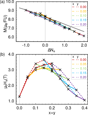
Figure 3: (a) Zero-temperature magnetization $M$ calculated as a function of electron number within the rigid band model (black dotted line) or using the CPA. (b) Anisotropy field $\mu_{0}H_{a}$ ($=2K/M$) obtained in the CPA, plotted as a function of dopant content $x+y$.

According to micromagnetic theory, the theoretical maximum for the coercive field of a ferromagnet is the anisotropy field, $\mu_{0}H_{a}=2K/M$ [59, 60]. Therefore, it is also important to investigate the dependence of the magnetization $M$ on doping, which is shown in Fig. 3(a).

In this case, there is quite close agreement between the rigid band model (black dotted line) and the CPA calculations. The moment calculated for pristine YCo₅ is 8.3$\mu_{B}$/FU, where $\mu_{B}$ is the Bohr magneton. Adding electrons to YCo₅ (Cu-doping) increases the population of the minority spin band, and therefore decreases the magnetization. The reverse applies when electrons are removed (Fe-doping). We note that, although the agreement is generally good, the magnetization decreases faster with Cu doping than predicted by the rigid band model. For instance, for YCo₄Cu the magnetization calculated with the CPA is 6.1 $\mu_{B}$/FU, compared to the rigid band prediction of 6.6 $\mu_{B}$/FU.

Figure 3(b) shows the anisotropy field calculated from the anisotropy energies and magnetizations in Figs. 2(b) and 3(a), respectively. Comparing to Fig. 2(b), we find a smaller scatter in $H_{a}$ compared to $K$ for different compositions. The reason for this smaller scatter is that the increased $K$ from doping with larger amounts of Fe is partly offset by the increased $M$; similarly, increasing the amount of Cu weakens $M$ and therefore helps to boost $H_{a}$. The clearest example is YCo₄Cu, whose value of $K$ is smaller than YCo₄Fe by a factor of 1.4 (0.61 vs. 0.86 meV/FU), but whose anisotropy field is actually larger (3.4 vs. 3.3 T). Nonetheless, the purely Fe-doped Y(Co_0.85Fe_0.15)₅ has both the highest anisotropy energy (0.93 meV/FU) and anisotropy field (3.6 T).

3.4 Dependence of anisotropy on site occupation

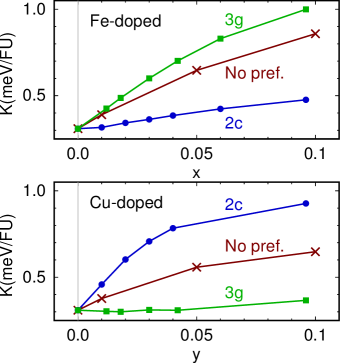
Figure 4: Anisotropy energies of Y(Co_1-xFe_x)₅ and Y(Co_1-yCu_y)₅ calculated with no preferential (pref.) substitution at particular sites, compared to exclusive substitution at the 2$c$ or 3$g$ crystal sites.

As stated already, the CPA calculations presented above were performed assuming both Cu and Fe substitute onto the 2$c$ and 3$g$ sites with equal probability. On the other hand, it is possible that the dopants may prefer to substitute at particular sites, and that the value of $K$ might be affected. Therefore, in Fig. 4 we compare the previous calculations of the anisotropy energy of Y(Co_1-xFe_x)₅ and Y(Co_1-yCu_y)₅ with the case where the dopants are placed exclusively at the 2$c$ or 3$g$ crystal sites (Fig. 1).

Interestingly, there is indeed a strong dependence of $K$ on the location of the dopants, with the site that gives the largest enhancement to the anisotropy depending on the dopant. Substituting Co with Cu at the 3$g$ site has essentially no effect on the anisotropy energy, while substituting with Fe at the 2$c$ site also does not result in a large change. By contrast, placing Cu at the 2$c$ site or Fe at the $3g$ site has a large effect on $K$. Substituting the dopants equally at both sites effectively interpolates between the two limiting cases.

We are unaware of experimental data directly characterizing the location of dopant atoms in Y(Co_1-xFe_x)₅ or Y(Co_1-yCu_y)₅. Neutron diffraction measurements on the related compounds Th(Co_1-xFe_x)₅ and Y(Co_1-yNi_y)₅ found preferential Fe/Ni substitution at the 3$g$/2$c$ sites, respectively [61, 62]. However based on the changes in lattice parameters in Y(Co_1-xFe_x)₅ with Fe doping it was argued in Ref. [63] that Fe preferred to occupy 2$c$ sites. Our own CPA calculations performed at zero temperature (ferromagnetic state) find $2c$ substitution to be preferred for Fe, Cu, and Ni [35] but calculations on stoichiometric systems including optimization of the lattice parameters found Fe to prefer 3$g$ doping and Cu to prefer 2$c$ [64]. Furthermore our test calculations and previous work [65] have shown the energetics to be sensitive to the modeling of the magnetic state (ferromagnetic versus nonmagnetic). For definiteness, in what follows we place Fe at 3$g$ sites and Cu at 2$c$ sites in line with the neutron data [61, 62], the calculations including geometry optimization [64] and with previous theoretical works [66, 67].

3.5 Anisotropy at zero temperature: CPA, preferential 3$g$/2$c$ substitution

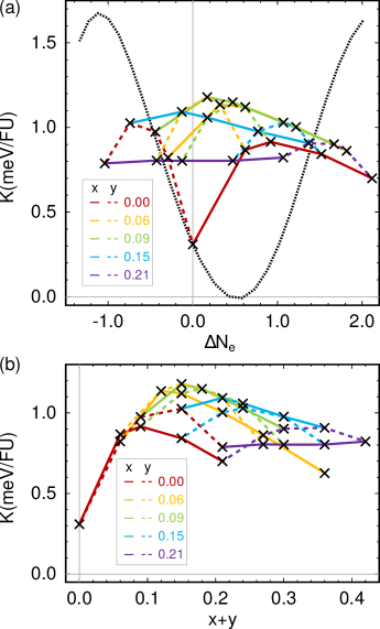
Figure 5: (a) Anisotropy energy $K$ of Y(Co_1-x-yFe_xCu_y)₅ calculated either in the rigid band approximation (black dotted line) or with the CPA (crosses) (cf. Fig. 2). The CPA calculations were performed placing Fe (Cu) at 3$g$ (2$c$) sites. (b) The same CPA calculations as (a) replotted as a function of dopant content $x+y$.

In Fig. 5(a) we plot $K$ calculated for Y(Co_1-x-yFe_xCu_y)₅ with the CPA, placing Fe at the 3$g$ sites and Cu at the 2$c$ sites. For comparison we show again the band-filling behavior predicted by the rigid band approximation (Sec. 3.1).

Referring to the data shown in Fig. 2(a), we see that the anisotropy energy is enhanced compared to non-preferential site substitution. The largest value of $K$, calculated for Y(Co_0.85Fe_0.09Cu_0.06)₅, is 1.18 meV/FU, whilst the smallest value (apart from pristine YCo₅) is calculated to be 0.70 meV/FU for Y(Co_0.79Cu_0.21)₅.

As with the calculations with non-preferential site substitution, the agreement between the rigid band and CPA calculations is poor. For instance, it is interesting to compare the sensitivity of $K$ to the level of Cu doping, at low and high Fe content. For Y(Co_1-yCu_y)₅ (red solid line), $K$ varies between 0.31 meV/FU at $y=0.00$ to a peak value of 0.92 meV/FU at $y=0.09$. However, including Fe at the level Y(Co_0.79-yFe_0.21Cu_y)₅ (purple solid line) reduces the variation in $K$ to just 0.03 meV/FU over the entire range of $y$.

Replotting the CPA calculations against $x+y$ [Fig. 5(b)] does not show as clear a trend as for the non-preferential doping case [Fig. 2(b)]. However, again it is found that the largest values of the anisotropy energy are calculated for concentrations with $x+y\sim 0.15$. Around this optimal level, the largest values of $K$ have similar Fe and Cu concentrations. By contrast, the Cu-rich Y(Co_0.85Cu_0.15)₅ has a relatively low $K$. However, at the lowest dopant concentrations $(x,y)=0.06$ the effect of replacing Co with either Cu or Fe is very similar.

3.6 Anisotropy fields at zero temperature: Cu-rich vs. equal Cu/Fe content

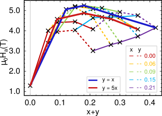
Figure 6: Anisotropy fields calculated within the CPA placing Fe (Cu) at 3$g$ (2$c$) sites. Additionally, calculations with equal Fe/Cu doping ($x=y$) and Cu-rich ($y=5x$) doping are shown with thick blue and red lines, respectively.

Unlike the anisotropy energy, the magnetization $M$ is not particularly sensitive on the location of the dopants, following the same behavior as shown in Fig. 3(a). In Fig. 6 we plot the anisotropy field for preferential substitution of Fe/Cu at the $3g$/2$c$ sites. As for the non-preferential case [Fig. 3(b)] the anisotropy field is enhanced (weakened) for large Cu (Fe) content, due to effect of the dopants on $M$. This can be seen most clearly for the composition discussed above, Y(Co_0.79-yFe_0.21Cu_y)₅, which has $K$ effectively independent of $y$ but $H_{a}$ which increases with Cu content due to the corresponding reduction in $M$.

Motivated by the observations made at the end of the previous section, Fig. 6(b) shows some additional data points, calculated for equal Fe/Cu doping ($x=y$; thick red line) and Cu-rich doping, which we define as $y=5x$ (thick blue line). Here, it can be seen that despite the boost to $H_{a}$ by the smaller magnetization of Cu, the compositions with equal amounts of Fe and Cu have larger anisotropy fields than the Cu-rich compositions. Of all of the compositions considered, Y(Co_0.82Fe_0.09Cu_0.09)₅ is found to have the highest anisotropy field of $\mu_{0}H_{a}$ = 5.3 T. The Cu-rich composition with the same $x+y$, Y(Co_0.82Fe_0.03Cu_0.15)₅, has $\mu_{0}H_{a}$ = 4.9 T.

3.7 Anisotropy at finite temperature: YCo₅, Y(Co_0.838Cu_0.162)₅ and Y(Co_0.838Fe_0.081Cu_0.081)₅

In order to make a tentative connection to the 2:17 Sm-Co magnets, we now focus on specific compositions similar to those reported for the cell-boundary phase in high and low coercivity samples in Ref. [25] and calculate their properties between 0–300 K. In Ref. [25], high coercivity was correlated with a Cu-rich cell-boundary phase, while low coercivity was correlated with equal Cu and Fe content. We model the two cases with compositions ($x$,$y$) = (0.00,0.162) and (0.081,0.081). We also compare to pristine YCo₅. As in Secs. 3.5 and 3.6 we place the Fe and Cu dopants at the 3$g$ and 2$c$ sites, respectively.

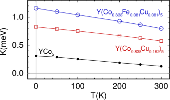
Figure 7: Anisotropy energy $K$ calculated for YCo₅ (black circles), Y(Co_0.838Cu_0.162)₅ (red squares) and Y(Co_0.838Fe_0.081Cu_0.081)₅ (blue circles) as a function of temperature.

Figure 7 shows the anisotropy energy $K$ calculated as a function of temperature $T$, for the three cases. As expected from Fig. 5, at zero temperature YCo₅ has the lowest $K$ value of 0.31 meV/FU, followed by Y(Co_0.838Cu_0.162)₅ (0.83 meV/FU) and then Y(Co_0.838Fe_0.081Cu_0.081)₅ (1.10 meV/FU). Up to at least $T=300~{}K$, this ordering is unchanged, with each composition showing a monotonic decrease in $K$ with temperature with a similar slope. At 300 K, the $K$ values for the three configurations are 0.12, 0.57 and 0.80 meV/FU respectively.

($x,y$)	$K$ (meV/FU)	$M$ ($\mu_{B}$/FU)	$\mu_{0}H_{a}$ (T)	$T_{\mathrm{C}}$ (K)
(0.000,0.000)	0.31 ; 0.12	8.14 ; 7.16	1.3 ; 0.6	841
(0.000,0.162)	0.83 ; 0.57	6.42 ; 5.52	4.4 ; 3.6	711
(0.081,0.081)	1.10 ; 0.80	7.63 ; 6.66	5.2 ; 4.1	788

Table 1: Anisotropy energy $K$, magnetization $M$, anisotropy field $H_{a}$ and Curie temperature $T_{\mathrm{C}}$ calculated for Y(Co_1-x-yFe_xCu_y)₅. The two values given for $K$, $M$ and $H_{a}$ correspond to calculations at $T$ = 0 and 300 K.

The magnetization and anisotropy field (not shown) display the same monotonic decrease with temperature. We also calculated the Curie temperatures $T_{\mathrm{C}}$, finding the largest value (841 K) for pristine YCo₅. The $T_{\mathrm{C}}$ of Y(Co_0.838Cu_0.162)₅ is found to be lower by over 100 K (711 K), while Y(Co_0.838Fe_0.081Cu_0.081)₅ lies in between (788 K). The temperature-dependent results are summarized in Table 1.

3.8 Deriving parameters for micromagnetics simulations

The quantities $K$, $M$ and $T_{\mathrm{C}}$ listed in Table 1 may be obtained directly from the DFT-DLM calculations. However micromagnetics simulations in fact require the magnetic polarization $J^{\mathrm{m}}$ and stiffness constant $A^{\mathrm{m}}$ in addition to the anisotropy $K^{\mathrm{m}}$ [26]. Denoting the volume per formula unit as $\Omega(=\sqrt{3}a^{2}c/2)$, the anisotropy and polarization can be straightforwardly related to the quantities given in Table 1:

$$K^{\mathrm{m}} = K/\Omega$$ (1)

$$J^{\mathrm{m}} = \mu_{0}M/\Omega$$ (2)

We again note that the derived $K^{\mathrm{m}}$ values are likely to be underestimates since no orbital polarization correction terms were included (Sec. 2).

($x,y$)	$K^{\mathrm{m}}$ (MJ/m3)	$J^{\mathrm{m}}$ (T)	$A^{\mathrm{m}}$ (pJ/m)
(0.000,0.000)	0.59 ; 0.23	1.12 ; 0.99	8.3 ; 6.6
(0.000,0.162)	1.57 ; 1.08	0.88 ; 0.76	7.0 ; 5.4
(0.081,0.081)	2.08 ; 1.52	1.05 ; 0.92	7.7 ; 6.1

Table 2: Anisotropy energy $K^{\mathrm{m}}$, magnetic polarization $J^{\mathrm{m}}$ and exchange stiffness constant $A^{\mathrm{m}}$ calculated for Y(Co_1-x-yFe_xCu_y)₅ as discussed in the text. The two values given correspond to calculations at $T$ = 0 and 300 K.

We have not yet established a formal framework to extract the exchange stiffness constant $A^{\mathrm{m}}$ from the DFT-DLM calculations. A similar challenge is encountered when performing calculations based on atomistic spin models [45]. In the current work we use a basic approximation [26, 27]:

$$A^{\mathrm{m}}=(k_{\mathrm{B}}T_{\mathrm{C}}/\Omega)\ \zeta^{2}\ [m_{\mathrm{Co}}(T)]^{2}$$ (3)

where $\zeta$ is the nearest neighbor distance between transition metal atoms and $m_{\mathrm{Co}}(T)$ is the calculated order parameter of the Co moments at temperature $T$. The results of using equations 1–3 to express the quantities in Table 1 as micromagnetics parameters are shown in Table 2.

3.9 Temperature in DFT-DLM calculations

We conclude this section by noting that the classical statistical mechanics used in the DLM picture leads to a faster decay of the the magnetic order parameter $m_{\mathrm{Co}}(T)$ with temperature than observed experimentally [68]. As a result, the DFT-DLM “temperature” may in fact correspond to a higher temperature in experiment. To illustrate this aspect, we note from our DFT-DLM calculations on YCo₅ that at a calculated temperature of 300 K, $m_{\mathrm{Co}}$ has a value of 0.90. However, the experimental data shown in Ref. [69] shows $m_{\mathrm{Co}}=0.90$ in fact corresponds to a temperature of 465 K. Conversely, at an experimental temperature of 300 K the order parameter is 0.95 [69], which in the DFT-DLM calculations corresponds to a temperature of 200 K. As illustrated here, it is relatively straightforward to correct for this effect if required by mapping the DFT-DLM order parameters onto the experimental magnetization versus temperature curves [69].

4 Discussion

Here we discuss the specific results presented in Sec. 3 in more general terms.

4.1 Modelling doping

We first highlight some limitations of our chosen method of simulating the doping. First, we have not attempted to include structural effects in our calculations, instead using the same lattice parameters for all concentrations. The anisotropy has previously been shown to be sensitive to the $c$/$a$ ratio [70], so different-sized dopants may affect $K$ indirectly in this way. In the context of understanding the cell-boundary phase in the 2:17 magnets modeling this effect is especially difficult, since there may be local strains which invalidate predictions based on Vegard’s law or total energy minimization [64].

Also, the CPA assumes the limit of a dilute alloy, with the dopants dispersed homogeneously throughout the host structure. As a result, effects from short-range ordering are not included [71], which may be especially important in understanding the low coercivity 2:17 Sm-Co sample which had a diffusive interface between the cell and cell boundary phase [25].

Finally, we note that we have assumed a perfect YCo₅ structure and not explored the role of point defects, e.g. the “dumbbell” substitution which replaces Y with a pair of Co atoms [10]. It is possible that Fe and Cu may interact with these defects in different ways.

4.2 Rigid band or CPA?

Within the limitations of the above model, we explored two methods of modeling doping, namely the rigid band model or the CPA. While the two models produce similar values for the magnetization $M$, the predicted values of $K$ differ substantially. The rigid band model predicts much larger variations in the anisotropy energy $K$ than the CPA. Indeed the rigid band model predicts that the addition of a small amount of Cu should reduce $K$, potentially yielding a perfectly soft magnet for YCo_4.75Cu_0.25. By contrast the CPA almost always predicts $K$ to increase regardless of the dopant species, especially if there is preferential substitution at particular crystal sites.

From the theoretical point of view, the CPA is the more rigorous approach [43]. As suggested by its name, the rigid band model cannot account for changes in the bandstructure induced by the addition of dopants. Furthermore if we take the view that the anisotropy depends not only on the dopant species but also on which site it occupies (as argued experimentally a number of decades ago [72] and observed in the CPA calculations, e.g. Fig. 4), we see that the rigid band model cannot provide a full account of the behavior of $K$.

4.3 Comparison to experiment

As noted in Sec. 2, since the current calculations do not include a correction for orbital polarization, we expect the calculated values of $K$ to be smaller than observed experimentally. Therefore we restrict our comparison to trends in $K$ with doping. We have not found experimental data on the ternary compound Y(Co_1-x-yFe_xCu_y)₅, but studies on the binaries Y(Co_1-xFe_x)₅ [63, 41, 73] and Y(Co_1-yCu_y)₅ [42] are available.

Considering Fe-doping first, Ref. [63] reports anisotropy constants at room temperature for $x$ = 0.0–0.3. Here $K$ increases from a value of 4.5 MJm^-3 for $x$ = 0.0 to a maximum of 5.5 MJm^-3 at $x$ = 0.10, before reducing again. Interestingly a follow-up work [41] states that there were calibration errors the original data, even though later papers continued to cite the original reference [72]. A more recent work [73] measured $K$ for $x$ = 0.0–0.15 and found an increase from 4.2 to 5.0 MJm^-3, (again at room temperature), reasonably consistent with Ref. [63].

So, for Fe doping there is at least qualitative agreement between different experiments and the current calculations in predicting an increased $K$ on the addition of a small amount of Fe. Quantitatively, the change of 0.8 MJm^-3 between $x=0.0$ and $x=0.15$ found in Ref. [73] corresponds to an absolute increase of approximately 0.4 meV/FU, or a relative increase of 19%. The (zero temperature) calculations predict an absolute increase of 0.7 meV/FU over the same composition range (Fig. 5), but a much larger relative increase of over 300%.

Now considering Cu doping, Ref. [42] reports anisotropy fields for Y(Co_1-yCu_y)₅ for $y$ = 0.0, 0.2 and 0.4, at temperatures $T>200$ K (lower temperature data are reported for $y=0.4$). At the studied temperature range, YCo₅ is reported to have the highest anisotropy field. However the difference between the pristine case and $y=0.2$ (YCo₄Cu) gets smaller with decreasing temperature, and a straightforward linear extrapolation of the data indicates the anisotropy field of YCo₄Cu would exceed YCo₅ at temperatures below 50 K. We were unable to find experimental data measured for lower Cu concentrations which could be compared more directly to our calculations. Such data, particularly at very low Cu concentration ($y\sim 0.05$) would be useful e.g. in comparing the rigid band model with the CPA, since the former predicts a perfectly soft magnet at this concentration (Fig. 2).

Finally, we note that although our calculations should ideally be compared to anisotropy constants measured for single crystals, there are a number of experiments which report coercivity enhancement in RE/TM magnets upon addition of Fe or Cu [74, 75, 76].

4.4 2:17 Sm-Co magnets

We return to the original motivation of our work, to quantify the effect on the TM contribution to the anisotropy with Fe and Cu doping. As shown by the blue and red lines in Figs. 6 and 7, and the numbers reported in Table 1 the differences between doping purely with Cu or with equal quantities of Cu and Fe are not particularly large. The anisotropy energy and field is calculated to be slightly smaller for Y(Co_0.838Cu_0.162)₅ compared to Y(Co_0.838Fe_0.081Cu_0.081)₅. This fact, combined with a lower exchange stiffness constant for Y(Co_0.838Cu_0.162)₅ (Table 2) gives a lower domain wall energy in this phase compared to Y(Co_0.838Fe_0.081Cu_0.081)₅ [26].

Applying this observation to a repulsive pinning model (where the 2:17 cells have smaller domain wall energies than the boundaries), one would expect stronger pinning for boundaries with the Y(Co_0.838Fe_0.081Cu_0.081)₅ composition. Unfortunately however, in Ref. [25] this composition (equal Fe and Cu content) corresponded to the low, not high, coercivity sample. Therefore, according to our calculations the TM contribution to the anisotropy does not account for the correlation of coercivity with the composition of the cell boundaries reported in Ref. [25]. Of course, as described in the Introduction the larger Sm contribution to the anisotropy may provide this missing link. In the final section we outline future work aimed at exploring the 2:17 magnets further.

5 Conclusions and outlook

The aim of this work has been to study how the magnetic anisotropy and magnetization of YCo₅ is affected when Co is substituted with Fe and/or Cu. We have demonstrated how two different approaches to modeling dopants — the rigid band model and the coherent potential approximation (CPA) — give rather different predictions. We also showed how the results of the CPA calculations depend very strongly on which crystal site the dopant atoms occupy.

Our CPA calculations found that the anisotropy of YCo₅ could be enhanced by adding reasonably small amounts of Fe and/or Cu, with the largest anisotropy field at zero temperature observed for the composition Y(Co_0.81Fe_0.09Cu_0.09)₅. Of the compositions studied, assuming preferential substitution of Fe and Cu at 3$g$ and 2$c$ sites respectively, Fe-rich samples (i.e. Y(Co_0.79-yFe_0.21Cu_y)₅) had the lowest anisotropy fields, but these still exceeded the anisotropy field of YCo₅ at zero temperature.

On the theoretical side, the obvious next step is to study the RE contribution to the anisotropy in Sm(Co_1-x-yFe_xCu_y)₅. In this case it will be essential to properly account for the crystal field effects in the calculations [77] and analyse the effects of hybridization of the $4f$ states with their environment [29, 36]. It will be interesting to see whether addition of a small quantity of Fe or Cu boosts the anisotropy like in YCo₅, or whether $K$ decreases for all compositions. In addition to the 1:5 calculations, a DFT-DLM characterization of the pristine bulk Y₂Co₁₇ and Sm₂Co₁₇ will be necessary to build a full picture of the cellular phase.

On the experimental side, first considering YCo₅, in our view the question of the site preference of the Fe-dopants has still not been conclusively answered. Having knowledge of this aspect would be a useful test both of using the CPA to calculate magnetic anisotropy, and also of total energy calculations in general to predict the preferred location of dopants. Furthermore, additional data exploring the behavior of $K$ for low Fe and Cu content, particularly for the ternary system, would also be useful. Complementary measurements on SmCo₅ are also required. In particular, as pointed out in Sec. 1, the experimental data exploring Cu-doped SmCo₅ does not extend to the critical $y<0.2$ region [27]. A full characterization of (Y,Sm)(Co_1-x-yFe_xCu_y)₅ for $(x,y)<0.2$ would therefore be a valuable contribution to the permanent magnet literature.

References

- [1] K. H. J. Buschow, Rep. Prog. Phys. 40 (1977) 1179. doi:10.1088/0034-4885/40/10/002.
- [2] M. Sagawa, S. Fujimura, N. Togawa, H. Yamamoto, Y. Matsuura, J. Appl. Phys. 55 (1984) 2083–2087. doi:10.1063/1.333572.
- [3] J. J. Croat, J. F. Herbst, R. W. Lee, F. E. Pinkerton, J. Appl. Phys. 55 (1984) 2078–2082. doi:10.1063/1.333571.
- [4] K. Strnat, G. Hoffer, J. Olson, W. Ostertag, J. J. Becker, J. Appl. Phys. 38 (1967) 1001–1002. doi:10.1063/1.1709459.
- [5] K. Strnat, IEEE Trans. Magn. 8 (1972) 511–516. doi:10.1109/TMAG.1972.1067368.
- [6] S. Chikazumi, Physics of Ferromagnetism, 2nd Edition, Oxford University Press, 1997.
- [7] O. Gutfleisch, M. A. Willard, E. Brück, C. H. Chen, S. G. Sankar, J. P. Liu, Adv. Mater. 23 (2011) 821–842. doi:10.1002/adma.201002180.
- [8] C. H. Chen, M. S. Walmer, M. H. Walmer, S. Liu, E. Kuhl, G. Simon, J. Appl. Phys. 83 (11) (1998) 6706–6708. doi:10.1063/1.367937.
- [9] O. Gutfleisch, High-Temperature Samarium Cobalt Permanent Magnets, Springer US, Boston, MA, 2009, pp. 337–372. doi:10.1007/978-0-387-85600-1_12.
- [10] K. Kumar, J. Appl. Phys. 63 (6) (1988) R13–R57. doi:10.1063/1.341084.
- [11] J. F. Liu, Y. Zhang, D. Dimitrov, G. C. Hadjipanayis, J. Appl. Phys. 85 (1999) 2800–2804. doi:10.1063/1.369597.
- [12] L. Rabenberg, R. K. Mishra, G. Thomas, J. Appl. Phys. 53 (3) (1982) 2389–2391. doi:10.1063/1.330867.
- [13] G. C. Hadjipanayis, W. Tang, Y. Zhang, S. T. Chui, J. F. Liu, C. Chen, H. Kronmüller, IEEE Trans. Magn. 36 (5) (2000) 3382–3387. doi:10.1109/20.908808.
- [14] M. Duerrschnabel, M. Yi, K. Uestuener, M. Liesegang, M. Katter, H.-J. Kleebe, B. Xu, O. Gutfleisch, L. Molina-Luna, Nat. Commun. 8 (1) (2017) 54. doi:10.1038/s41467-017-00059-9.
- [15] J. Fidler, J. Magn. Magn. Mater. 30 (1) (1982) 58 – 70. doi:10.1016/0304-8853(82)90010-5.
- [16] H. Kronmüller, D. Goll, Physica B 319 (1) (2002) 122 – 126. doi:10.1016/S0921-4526(02)01113-4.
- [17] D. Goll, H. Kronmüller, High-performance permanent magnets, Naturwissenschaften 87 (10) (2000) 423–438. doi:10.1007/s001140050755.
- [18] J. D. Livingston, D. L. Martin, J. Appl. Phys. 48 (3) (1977) 1350–1354. doi:10.1063/1.323729.
- [19] X. Xiong, T. Ohkubo, T. Koyama, K. Ohashi, Y. Tawara, K. Hono, Acta Mater. 52 (3) (2004) 737 – 748. doi:10.1016/j.actamat.2003.10.015.
- [20] H. Nagel, J. Appl. Phys. 50 (2) (1979) 1026–1030. doi:10.1063/1.326100.
- [21] K. Durst, H. Kronmüller, W. Ervens, Phys. Status Solidi A 108 (1) (1988) 403–416. doi:10.1002/pssa.2211080143.
- [22] B. Streibl, J. Fidler, T. Schrefl, J. Appl. Phys. 87 (9) (2000) 4765–4767. doi:10.1063/1.373152.
- [23] A. Yan, O. Gutfleisch, T. Gemming, K.-H. Müller, Appl. Phys. Lett. 83 (11) (2003) 2208–2210. doi:10.1063/1.1611641.
- [24] R. Gopalan, K. Hono, A. Yan, O. Gutfleisch, Scr. Mater. 60 (9) (2009) 764 – 767. doi:10.1016/j.scriptamat.2009.01.006.
- [25] H. Sepehri-Amin, J. Thielsch, J. Fischbacher, T. Ohkubo, T. Schrefl, O. Gutfleisch, K. Hono, Acta Mater. 126 (2017) 1. doi:10.1016/j.actamat.2016.12.050.
- [26] A. Hubert, R. Schäfer, Magnetic Domains, Springer-Verlag, 1998.
- [27] E. Lectard, C. H. Allibert, R. Ballou, J. Appl. Phys. 75 (10) (1994) 6277–6279. doi:10.1063/1.355423.
- [28] M. D. Kuz’min, A. M. Tishin, Vol. 17, Elsevier B.V., 2008, Ch. 3, p. 149.
- [29] C. E. Patrick, J. B. Staunton, Phys. Rev. B 97 (2018) 224415. doi:10.1103/PhysRevB.97.224415.
- [30] L. Nordstrom, M. S. S. Brooks, B. Johansson, J. Phys.: Condens. Matter 4 (12) (1992) 3261. doi:10.1088/0953-8984/4/12/016.
- [31] G. H. O. Daalderop, P. J. Kelly, M. F. H. Schuurmans, Phys. Rev. B 53 (1996) 14415–14433. doi:10.1103/PhysRevB.53.14415.
- [32] L. Steinbeck, M. Richter, H. Eschrig, Phys. Rev. B 63 (2001) 184431. doi:10.1103/PhysRevB.63.184431.
- [33] P. Larson, I. Mazin, J. Magn. Magn. Mater. 269 (2) (2004) 176 – 183. doi:10.1016/S0304-8853(03)00589-4.
- [34] M. Matsumoto, R. Banerjee, J. B. Staunton, Phys. Rev. B 90 (2014) 054421. doi:10.1103/PhysRevB.90.054421.
- [35] C. E. Patrick, S. Kumar, G. Balakrishnan, R. S. Edwards, M. R. Lees, E. Mendive-Tapia, L. Petit, J. B. Staunton, Phys. Rev. Materials 1 (2017) 024411. doi:10.1103/PhysRevMaterials.1.024411.
- [36] T. Miyake, H. Akai, J. Phys. Soc. Jpn 87 (4) (2018) 041009. doi:10.7566/JPSJ.87.041009.
- [37] K. Skokov, O. Gutfleisch, Scr. Mater. 154 (2018) 289 – 294. doi:10.1016/j.scriptamat.2018.01.032.
- [38] J. M. Alameda, D. Givord, R. Lemaire, Q. Lu, J. Appl. Phys. 52 (3) (1981) 2079–2081. doi:10.1063/1.329622.
- [39] A. Gabay, X. Hu, G. Hadjipanayis, J. Magn. Magn. Mater. 368 (2014) 75 – 81. doi:10.1016/j.jmmm.2014.05.014.
- [40] M. Soderžnik, M. Korent, K. Žagar Soderžnik, J.-M. Dubois, P. Tozman, M. Venkatesan, J. Coey, S. Kobe, J. Magn. Magn. Mater. 460 (2018) 401 – 408. doi:10.1016/j.jmmm.2018.04.036.
- [41] W. E. Wallace, E. V. Ganapathy, R. S. Craig, J. Appl. Phys. 50 (B3) (1979) 2327–2329. doi:10.1063/1.326990.
- [42] J. C. Tellez-Blanco, R. Grossinger, R. S. Turtelli, E. Estevez-Rams, IEEE Trans. Magn. 36 (2000) 3333–3335. doi:10.1109/20.908790.
- [43] B. L. Györffy, G. M. Stocks, Springer US, 1979, Ch. 4, pp. 89–192.
- [44] B. L. Györffy, A. J. Pindor, J. Staunton, G. M. Stocks, H. Winter, J. Phys. F: Met. Phys. 15 (1985) 1337. doi:10.1088/0305-4608/15/6/018.
- [45] Y. Toga, M. Nishino, S. Miyashita, T. Miyake, A. Sakuma, Phys. Rev. B 98 (2018) 054418. doi:10.1103/PhysRevB.98.054418.
- [46] T. Fukazawa, H. Akai, Y. Harashima, T. Miyake, J. Magn. Magn. Mater. 469 (2019) 296 – 301. doi:10.1016/j.jmmm.2018.08.071.
- [47] H. Ebert, D. Ködderitzsch, J. Minár, Rep. Prog. Phys. 74 (9) (2011) 096501. doi:10.1088/0034-4885/74/9/096501.
- [48] S. H. Vosko, L. Wilk, M. Nusair, Can. J. Phys. 58 (1980) 1200–1211. doi:10.1139/p80-159.
- [49] M. Däne, M. Lüders, A. Ernst, D. Ködderitzsch, W. M. Temmerman, Z. Szotek, W. Hergert, J. Phys.: Condens. Matter 21 (2009) 045604. doi:10.1088/0953-8984/21/4/045604.
- [50] A. V. Andreev, Vol. 8, Elsevier North-Holland, New York, 1995, Ch. 2, p. 59.
- [51] P. Strange, J. Staunton, B. L. Györffy, J. Phys. C: Solid State Phys. 17 (19) (1984) 3355. doi:10.1088/0022-3719/17/19/011.
- [52] P. Strange, Relativistic Quantum Mechanics, Cambridge University Press, 1998.
- [53] X. Wang, R. Wu, D.-s. Wang, A. J. Freeman, Phys. Rev. B 54 (1996) 61–64. doi:10.1103/PhysRevB.54.61.
- [54] J. B. Staunton, L. Szunyogh, A. Buruzs, B. L. Gyorffy, S. Ostanin, L. Udvardi, Phys. Rev. B 74 (2006) 144411. doi:10.1103/PhysRevB.74.144411.
- [55] E. Bruno, B. Ginatempo, Phys. Rev. B 55 (1997) 12946–12955. doi:10.1103/PhysRevB.55.12946.
- [56] O. Eriksson, B. Johansson, R. C. Albers, A. M. Boring, M. S. S. Brooks, Phys. Rev. B 42 (1990) 2707–2710. doi:10.1103/PhysRevB.42.2707.
- [57] H. Ebert, M. Battocletti, Solid State Commun. 98 (9) (1996) 785 – 789. doi:10.1016/0038-1098(96)00202-5.
- [58] C. E. Patrick, S. Kumar, G. Balakrishnan, R. S. Edwards, M. R. Lees, L. Petit, J. B. Staunton, Phys. Rev. Lett. 120 (2018) 097202. doi:10.1103/PhysRevLett.120.097202.
- [59] W. F. Brown, Phys. Rev. 105 (1957) 1479–1482. doi:10.1103/PhysRev.105.1479.
- [60] H. Kronmüller, Phys. Status Solidi B 144 (1987) 385–396. doi:10.1002/pssb.2221440134.
- [61] J. Deportes, D. Givord, J. Schweizer, F. Tasset, IEEE Trans. Magn. 12 (6) (1976) 1000–1002. doi:10.1109/TMAG.1976.1059185.
- [62] J. Laforest, J. Shah, IEEE Trans. Magn. 9 (3) (1973) 217–220. doi:10.1109/TMAG.1973.1067699.
- [63] F. Rothwarf, H. A. Leupold, J. Greedan, W. E. Wallace, D. K. Das, Int. J. Magnetism 4 (1973) 267–271.
- [64] K. Uebayashi, K. Terao, H. Yamada, J Alloys Compd 346 (2002) 47 – 49. doi:10.1016/S0925-8388(02)00516-9.
- [65] A. M. Gabay, P. Larson, I. I. Mazin, G. C. Hadjipanayis, J. Phys. D: Appl. Phys. 38 (9) (2005) 1337. doi:10.1088/0022-3727/38/9/002.
- [66] P. Larson, I. I. Mazin, D. A. Papaconstantopoulos, Phys. Rev. B 69 (2004) 134408. doi:10.1103/PhysRevB.69.134408.
- [67] A. Sakuma, J. Appl. Phys. 99 (8) (2006) 08J307. doi:10.1063/1.2176316.
- [68] C. E. Patrick, S. Kumar, K. Götze, M. J. Pearce, J. Singleton, G. Rowlands, G. Balakrishnan, , M. R. Lees, P. A. Goddard, J. B. Staunton, J. Phys.: Condens. Matter 30 (2018) 32LT01. doi:10.1088/1361-648X/aad029.
- [69] M. D. Kuz’min, Phys. Rev. Lett. 94 (2005) 107204. doi:10.1103/PhysRevLett.94.107204.
- [70] L. Steinbeck, M. Richter, H. Eschrig, J. Magn. Magn. Mater. 226–230, Part 1 (2001) 1011 – 1013. doi:10.1016/S0304-8853(00)01189-6.
- [71] S. N. Khan, J. B. Staunton, G. M. Stocks, Phys. Rev. B 93 (2016) 054206. doi:10.1103/PhysRevB.93.054206.
- [72] N. Thuy, J. Franse, N. Hong, T. Hien, J. Phys. Colloq. 49 (C8) (1988) C8–499–C8–504. doi:10.1051/jphyscol:19888227.
- [73] B. Das, B. Balamurugan, W. Zhang, S. V. J. S. R. Skomski, E.S. Krage, D. Sellmyer, REPM’12 - Proceedings of the 22nd International Workshop on Rare-Earth Permanent Magnets and their Applications 3 (2012) 427.
- [74] P. Tozman, M. Venkatesan, G. A. Zickler, J. Fidler, J. M. D. Coey, Appl. Phys. Lett. 107 (3) (2015) 032405. doi:10.1063/1.4927306.
- [75] R. M. Grechishkin, M. S. Kustov, O. Cugat, J. Delamare, G. Poulin, D. Mavrudieva, N. M. Dempsey, Appl. Phys. Lett. 89 (12). doi:10.1063/1.2347282.
- [76] K. H. J. Buschow, M. Brouha, J. Appl. Phys. 47 (4) (1976) 1653–1656. doi:10.1063/1.322787.
- [77] K. Hummler, M. Fähnle, Phys. Rev. B 53 (1996) 3272–3289. doi:10.1103/PhysRevB.53.3272.