A Unified Approach for Solving Sequential Selection Problems

Abstract

In this paper we develop a unified approach for solving a wide class of sequential selection problems. This class includes, but is not limited to, selection problems with no–information, rank–dependent rewards, and considers both fixed as well as random problem horizons. The proposed framework is based on a reduction of the original selection problem to one of optimal stopping for a sequence of judiciously constructed independent random variables. We demonstrate that our approach allows exact and efficient computation of optimal policies and various performance metrics thereof for a variety of sequential selection problems, several of which have not been solved to date.

Keywords: sequential selection, optimal stopping, secretary problems, relative ranks, full information problems, no–information problems.

2000 AMS Subject Classification: 60G40, 62L15

1 Introduction

In sequential selection problems a decision maker examines a sequence of observations which appear in random order over some horizon. Each observation can be either accepted or rejected, and these decisions are irrevocable. The objective is to select an element in this sequence to optimize a given criterion. A classical example is the so-called secretary problem in which the objective is to maximize the probability of selecting the element of the sequence that ranks highest. The existing literature contains numerous settings and formulations of such problems, see, e.g., GiMo, freeman, gnedin-book, ferguson, samuels and F2008; to make more concrete connections we defer further references to the subsequent section where we formulate the class of problems more precisely.

Sequential selection problems are typically solved using the principles of dynamic programming, relying heavily on structure that is problem-specific, and focusing on theoretical properties of the optimal solution; cf. GiMo, gnedin-book and F2008. Consequently, it has become increasingly difficult to discern commonalities among the multitude of problem variants and their solutions. Moreover, the resulting optimal policies are often viewed as difficult to implement, and focus is placed on deriving sub–optimal policies and various asymptotic approximations; see, e.g., mucci-a, FrSa, krieger-ester, and Arlotto, among many others.

In this paper we demonstrate that a wide class of such problems can be solved optimally and in a unified manner. This class includes, but is not limited to, sequential selection problems with no–information, rank–dependent rewards and allows for fixed or random horizons. The proposed solution methodology covers both problems that have been worked out in the literature, albeit in an instance-specific manner, as well as several problems whose solution to the best of our knowledge is not known to date. We refer to Section 2 for details. The unified framework we develop is based on the fact that various sequential selection problems can be reduced, via a conditioning argument, to a problem of optimal stopping for a sequence of independent random variables that are constructed in a special way. The latter is an instance of a more general class of problems, referred to as sequential stochastic assignments, first formulated and solved by DLR (some extensions are given in albright). The main idea of the proposed framework was briefly sketched in [Section 4]GZ; in this paper it is fully fleshed and adapted to the range of problems alluded to above.

The approach we take is operational, insofar as it supports exact and efficient computation of the optimal policies and corresponding optimal values, as well as various other performance metrics. In the words of robbins70, we “put the problem on a computer.” Optimal stopping rules that result from our approach belong to the class of memoryless threshold policies and hence have a relatively simple structure. In particular, the proposed reduction constructs a new sequence of independent random variables, and the optimal rule is to stop the first time instant when the current “observation” exceeds a given threshold. The threshold computation is predicated on the structure of the policy in sequential stochastic assignment problems à la DLR and albright (as part of the so pursued unification, these problems are also extended in the present paper to the case of a random time horizon). The structure of the optimal stopping rule we derive allows us to explicitly compute probabilistic characteristics and various performance metrics of the stopping time, which, outside of special cases, are completely absent from the literature.

The rest of the paper is structured as follows. Section 2 discusses sequential selection problems. In this section we formulate two general no–information problems with rank–dependent reward corresponding to fixed and random horizon [Problems (A1) and (A2) respectively]. We also present various specific problem instances, Problems (P1)–(P12), that are covered by the proposed unified framework. Section 3 describes the class of stochastic sequential selection problems: we consider the standard formulation, Problem (AP1), first introduced and solved by DLR, and a formulation with random horizon, Problem (AP2). These problems are central to our solution approach. Section 4 presents the auxiliary stopping problem, Problem (B), and explains its solution via the mapping to a stochastic assignment problem. It then explains the details of the reduction and the structure of the algorithm that implements our proposed stopping rule. Section 5 presents the implementation of said algorithm to Problems (P1)–(P12) surveyed in Secton 2. We close with a few concluding remarks in Section 6.

2 Sequential selection problems

Let us introduce some notation and terminology. Let $X_{1},X_{2},\ldots$ be an infinite sequence of independent identically distributed continuous random variables defined on a probability space $(\Omega,{\mathscr{F}},\mathrm{P})$. Let $R_{t}$ be the relative rank of $X_{t}$ and $A_{t,n}$ be the absolute rank of $X_{t}$ among the first $n$ observations (which we also refer to as the problem horizon):

$$R_{t}:=\sum_{j=1}^{t}{\bf 1}(X_{t}\leq X_{j}),\;\;A_{t,n}:=\sum_{j=1}^{n}{\bf 1}(X_{t}\leq X_{j}),\;\;\;t=1,\ldots,n.$$ (1)

Note that with this notation the largest observation has the absolute rank one, and $R_{t}=A_{t,t}$ for any $t$. Let ${\mathscr{R}}_{t}:=\sigma(R_{1},\ldots,R_{t})$ and ${\mathscr{X}}_{t}:=\sigma(X_{1},\ldots,X_{t})$ denote the $\sigma$–fields generated by $R_{1},\ldots,R_{t}$ and $X_{1},\ldots,X_{t}$, respectively; ${\mathscr{R}}=({\mathscr{R}}_{t},1\leq t\leq n)$ and ${\mathscr{X}}=({\mathscr{X}}_{t},1\leq t\leq n)$ are the corresponding filtrations. In general, the class of all stopping times of a filtration ${\mathscr{Y}}=({\mathscr{Y}}_{t},1\leq t\leq n)$ will be denoted ${\mathscr{T}}({\mathscr{Y}})$; i.e., $\tau\in{\mathscr{T}}({\mathscr{Y}})$ if $\{\tau=t\}\in{\mathscr{Y}}_{t}$ for all $1\leq t\leq n$.

Sequential selection problems are classified according to the information available to the decision maker and the structure of the reward function. The settings in which only relative ranks $\{R_{t}\}$ are observed are usually referred to as no–information problems, whereas full information refers to the case when random variables $\{X_{t}\}$ can be observed, and their distribution is known. In addition, the total number of available observations $n$ can be either fixed or random with given distribution. These cases are referred to as problems with fixed and random horizon, respectively.

2.1 Problems with fixed horizon

In this paper we mainly consider selection problems with no–information and rank–dependent reward. The prototypical sequential selection problem with fixed horizon, no–information and rank–dependent reward is formulated as follows; see, e.g., gnedin-krengel.

Problem (A1). Let $n$ be a fixed positive integer, and let $q:\{1,2,\ldots,n\}\to{\mathbb{R}}$ be a reward function. The average reward of a stopping rule $\tau\in{\mathscr{T}}({\mathscr{R}})$ is

$$V_{n}(q;\tau):=\mathrm{E}q\big{(}A_{\tau,n}\big{)}.$$

The objective is to find the rule $\tau_{*}\in{\mathscr{T}}({\mathscr{R}})$ satisfying

$$V^{*}_{n}(q):=\max_{\tau\in{\mathscr{T}}({\mathscr{R}})}V_{n}(q;\tau)=\mathrm{E}q\big{(}A_{{\tau_{*},n}}\big{)}$$

and to compute the optimal value $V^{*}_{n}(q)$.

Depending on the reward function $q$ we distinguish among the following types of sequential selection problems with fixed horizon.

Best–choice problems.

The settings in which the reward function is an indicator are usually referred to as best–choice stopping problems. Of special note are the following.

(P1). Classical secretary problem. This problem setting corresponds to the case $q(a)=q_{\rm csp}(a):={\bf 1}\{a=1\}$. Here we want to maximize the probability $\mathrm{P}\{A_{\tau,n}=1\}$ of selecting the best alternative over all stopping times $\tau$ from ${\mathscr{T}}({\mathscr{R}})$. It is well known that the optimal policy will pass on approximately the first $n/e$ observations and select the first subsequent to that which is superior than all previous ones, if such an observation exists; otherwise the last element in the sequence is selected. The limiting optimal value is $\lim_{n\to\infty}V^{*}_{n}(q_{\rm csp})=1/e$ [lindley, Dyn, GiMo]. Ferguson (1989) reviews the problem history and discusses how different assumptions about this problem evolved over time.

(P2). Selecting one of the $k$ best values. The problem is usually referred to as the Gusein–Zade stopping problem [GuZa, FrSa]. Here $q(a)=q_{\rm gz}^{(k)}(a):={\bf 1}\{a\leq k\}$, and the problem is to maximize $\mathrm{P}\{A_{\tau,n}\leq k\}$ with respect to $\tau\in{\mathscr{T}}({\mathscr{R}})$. The optimal policy was characterized in GuZa. It is determined by $k$ natural numbers $1\leq\pi_{1}\leq\cdots\leq\pi_{k}$ and proceeds as follows: pass the first $\pi_{1}-1$ observations and among the subsequent $\pi_{1},\pi_{1}+1,\ldots,\pi_{2}-1$ observations choose the first observation with relative rank one; if it does not exists then among the set of observations $\pi_{2},\pi_{2}+1,\ldots,\pi_{3}-1$ choose the one of relative rank two, etc. GuZa presented dynamic programming algorithm to determine the numbers $\pi_{1},\ldots,\pi_{k}$ and value of $V^{*}_{n}(q_{\rm gz}^{(k)})$. He also studied the limiting behavior of the numbers $\pi_{1},\ldots,\pi_{k}$ as the problem horizon grows large, and showed that $\lim_{n\to\infty}V^{*}_{n}(q_{\rm gz}^{(2)})\approx 0.574$. Exact results for the case $k=3$ are given in QuLaw and for general $k$ in Woryna2017.

Based on general asymptotic results of mucci-a, FrSa computed numerically $\lim_{n\to\infty}V^{*}_{n}\big{(}q_{\rm gz}^{(k)}\big{)}$ for a range of different values of $k$. The recent paper DiLaRi studies some approximate policies.

(P3). Selecting the $k$th best alternative. In this problem $q(a)=q_{\rm pd}^{(k)}(a):={\bf 1}\{a=k\}$, i.e. we want to maximize the probability of selecting the $k$th best candidate. The problem was explicitly solved for $k=2$ by Szajowski1982, Rose and Vanderbei2012; the last paper coined the name the postdoc problem for this setting. An optimal policy for $k=2$ is to reject first $\lceil n/2\rceil$ observations and then select the one which is the second best relative to this previous observation set, if it exits; otherwise the last element in the sequence is selected. The optimal value is $V^{*}_{n}(q_{\rm pd}^{(2)})=(n+1)/4n$ if $n$ is odd and $V^{*}_{n}(q_{\rm pd}^{(2)})=n/4(n-1)$ if $n$ is even. An optimal stopping rule for the case $k=3$ and some results on the optimal value were reported recently in Yao. We are not aware of results on the optimal policy and exact computation of the optimal values for general $n$ and $k$. Recently approximate policies were developed in Bruss-2016. The problem of selecting the median value $k=(n+1)/2$, where $n$ is odd, was considered in Rose-2. It is shown there that $\lim_{n\to\infty}V^{*}_{n}(q_{\rm pd}^{((n+1)/2)})=0$.

Expected rank type problems.

To this category we attribute problems with reward $q$ which is not an indicator function.

(P4). Minimization of the expected rank. In this problem the goal is to minimize $\mathrm{E}A_{\tau,n}$ with respect to $\tau\in{\mathscr{T}}({\mathscr{R}})$. If we put $q(a)=q_{\rm er}(a):=-a$ then

$$\min_{\tau\in{\mathscr{T}}({\mathscr{R}})}\mathrm{E}A_{\tau,n}=-\max_{\tau\in{\mathscr{T}}({\mathscr{R}})}\mathrm{E}\,q_{\rm er}(A_{\tau,n}).$$ (2)

This problem was discussed heuristically by lindley and solved by chow. It was shown there that $\lim_{n\to\infty}\min_{\tau\in{\mathscr{T}}({\mathscr{R}})}\mathrm{E}A_{\tau,n}=\prod_{j=1}^{\infty}(1+\frac{2}{j})^{1/(j+1)}\approx 3.8695$. The corresponding optimal stopping rule is given by backward induction relations. A simple suboptimal stopping rule which is close to the optimal one was proposed in krieger-ester.

(P5). Minimization of the expected squared rank. Based on chow, Robbins-91 developed the optimal policy and computed the asymptotic optimal value in the problem of minimization of $\mathrm{E}[A_{\tau,n}(A_{\tau,n}+1)\cdots(A_{\tau,n}+k-1)]$ with respect to $\tau\in{\mathscr{T}}({\mathscr{R}})$. In particular, he showed that for the optimal stopping rule $\tau_{*}$

$$\lim_{n\to\infty}\mathrm{E}[A_{\tau_{*},n}(A_{\tau_{*},n}+1)\cdots(A_{\tau_{*},n}+k-1)]=k!\bigg{\{}\prod_{j=1}^{\infty}\bigg{(}1+\frac{k+1}{j}\bigg{)}^{1/(k+j)}\bigg{\}}^{k}.$$

Robbins-91 also discussed the problem of minimization of $\mathrm{E}A^{2}_{\tau,n}$ over $\tau\in{\mathscr{T}}({\mathscr{R}})$ and mentioned that the optimal stopping rule and optimal value are unknown. As we will demonstrate below, optimal policies for any problem of this type can be easily derived, and the corresponding optimal values are straightforwardly calculated for any fixed $n$.

2.2 Problems with random horizon

In Problem (A1) and specific problem instances of Section 2.1 the horizon $n$ is fixed beforehand, and optimal policies depend critically on this assumption. However, in practical situations $n$ may be unknown. This fact motivates settings in which the horizon is assumed to be a random variable.

If the horizon is random then the selection may not have been made by the time the observation process terminates. In order to take this possibility into account, we introduce minor modifications in the definitions of the absolute and relative ranks in (1). By convention we put $A_{t,k}=0$ for $t>k$, and if $N$ is a positive random variable representing the problem horizon and taking values in $\{1,\ldots,N_{\max}\}$ ($N_{\max}$ can be infinite) then on the event $\{N=k\}$, $k=1,\ldots,N_{\max}$, we set

$$\bar{R}_{t}:=\left\{\begin{array}[]{ll}R_{t},&t=1,\ldots,k,\\ 0&t=k+1,\ldots,N_{\max}.\end{array}\right.$$ (3)

Furthermore, $\bar{{\mathscr{R}}}_{t}:=\sigma(\bar{R}_{1},\dots,\bar{R}_{t})$ denotes the $\sigma$–field induced by $(\bar{R}_{1},\ldots,\bar{R}_{t})$, and $\bar{{\mathscr{R}}}:=\{\bar{{\mathscr{R}}}_{t},1\leq t\leq N_{\max}\}$ is the corresponding filtration. We refer to the sequence $\{\bar{R}_{t},1\leq t\leq N_{\max}\}$ as the sequence of observed relative ranks.

The general selection problem with random horizon, no–information and rank–dependent reward is formulated as follows [see PS1972 and Irle80].

Problem (A2). Let $N$ be a positive integer random variable with distribution $\gamma=\{\gamma_{k}\}$, $\gamma_{k}=\mathrm{P}(N=k)$, $k=1,2,\ldots,N_{\max}$, where $N_{\max}$ may be infinite. Assume that $N$ is independent of the sequence $\{X_{t},t\geq 1\}$. Let $q:\{1,\ldots,N_{\max}\}\cup\{0\}\to[0,\infty)$ be a reward function, and by convention $q(0)=0$. Let $Q_{t}:=q(A_{t,k})$, $t\in\{1,\ldots,N_{\max}\}$ on the event $\{N=k\}$. The performance of a stopping rule $\tau\in{\mathscr{T}}(\bar{{\mathscr{R}}})$ is measured by $V_{\gamma}(q;\tau):=\mathrm{E}Q_{\tau}$. The objective is to find the stopping rule $\tau_{*}\in{\mathscr{T}}(\bar{{\mathscr{R}}})$ such that

$$V_{\gamma}^{*}(q):=\max_{\tau\in{\mathscr{T}}(\bar{{\mathscr{R}}})}\mathrm{E}Q_{\tau}=\max_{\tau\in{\mathscr{T}}(\bar{{\mathscr{R}}})}V_{\gamma}(q;\tau)=V_{\gamma}(q;\tau_{*})$$

and to compute the optimal value $V^{*}_{\gamma}(q)$.

The introduced model assigns fictitious zero value to the observed relative rank $\bar{R}_{t}$ if the selection has not been made by the end of the problem horizon, i.e., if $t>N$. By assumption $q(0)=0$ the reward for not selecting an observation by time $N$ is also set to zero, though other possibilities can be considered for this value.

In principle, all problems (P1)–(P5) discussed above can be formulated and solved under the assumption that the observation horizon is random. Below we discuss the following three problem instances.

(P6). Classical secretary problem with random horizon. The classical secretary problem with random horizon $N$ corresponds to Problem (A2) with $q(a)={\bf 1}\{a=1\}$; it was studied in PS1972. In Problem (P1) where $n$ is fixed, the stopping region is an interval of the form $\{k_{n},\ldots,n\}$ for some integer $k_{n}$. In contrast to (P1), PS1972 show that for general distributions of $N$ the optimal policy can involve “islands,” i.e., the stopping region can be a union of several disjoint intervals (“islands”). The paper derives some sufficient conditions under which the stopping region is a single interval and presents specific examples satisfying these conditions. In particular, it is shown that in the case of the uniform distribution on $\{1,\ldots,N_{\max}\}$, i.e., $\gamma_{k}=1/N_{\max}$, $k=1,\ldots,N_{\max}$, the stopping region is of the form $\{k_{N_{\max}},\ldots,N_{\max}\}$ with $k_{N_{\max}}/N_{\max}\to 2e^{-2}$, $V^{*}_{\gamma}(q_{\rm csp})\to 2e^{-2}$ as $N_{\max}\to\infty$. The characterization of optimal policies for general distributions of $N$ is not available in the existing literature.

(P7). Selecting one of the $k$ best values over a random horizon. This is a version of the Gusein–Zade stopping problem, Problem (P2), with random horizon. Recall that here the reward function is $q_{\rm gz}^{(k)}(a)={\bf 1}\{a\leq k\}$. To the best of our knowledge, this setting has been studied only for $k=2$ and uniform distribution of $N$, i.e., $\gamma_{k}=1/N_{\max}$, $k\in\{1,\ldots,N_{\max}\}$; see KT2003. The cited paper derives the optimal policy and demonstrates that it is qualitatively the same as in the setting with fixed horizon. KT2003 study asymptotics of thresholds $\pi_{1}$ and $\pi_{2}$, and compute numerically the problem optimal value for a range of $N_{\max}$’s; in particular, $\lim_{N_{\max}\to\infty}V^{*}_{\gamma}(q_{\rm gz}^{(2)})\approx 0.4038$. Below we show how this problem can be stated and solved for general $k$ and arbitrary distribution of $N$ within our proposed unified framework.

(P8). Minimization of the expected rank over a random horizon. Consider a variant of Problem (P4) under the assumption that the horizon is a random variable $N$ with known distribution. In this setting the loss (the negative reward) for stopping at time $t$ is the absolute rank $A_{t,N}$ on the event $\{N\geq t\}$; otherwise, the absolute rank of the last available observation $A_{N,N}=R_{N}$ is received. We want to minimize the expected loss over all stopping rules $\tau\in{\mathscr{T}}(\bar{{\mathscr{R}}})$. This problem has been considered in Gianini-Pettitt. In particular, it was shown there that if $N$ is uniformly distributed over $\{1,\ldots,N_{\max}\}$ then the expected loss tends to infinity as $N_{\max}\to\infty$. On the other hand, for distributions which are more “concentrated” around $N_{\max}$, the optimal value coincides asymptotically with the one for Problem (P4). Below we demonstrate that this problem can be naturally formulated and solved for general distributions of $N$ using our proposed unified framework; the details are given in Section 5.2.3.

2.3 Multiple choice problems

The proposed framework is also applicable for some multiple choice problems both with fixed and random horizons. Below we review two settings with fixed horizon.

(P9). Maximizing the probability of selecting the best observation with $k$ choices. Assume that one can make $k$ selections, and the reward function equals one if the best observation belongs to the selected subset and zero otherwise. Formally, the problem is to maximize the probability $\mathrm{P}(\cup_{j=1}^{k}\{A_{\tau_{j},n}=1\})$ over stopping times $\tau_{1}<\cdots<\tau_{k}$ from ${\mathscr{T}}({\mathscr{R}})$. This problem has been considered in GiMo who gave numerical results for up to $k=8$; see also Haggstrom for theoretical results for $k=2$.

(P10). Minimization of the expected average rank. Assume that $k$ choices are possible, and the goal is to minimize the expected average rank of the selected subset. Formally, the problem is to minimize $\frac{1}{k}\mathrm{E}\sum_{j=1}^{k}A_{\tau_{j},n}$ over stopping times $\tau_{1}<\cdots<\tau_{k}$ of ${\mathscr{T}}({\mathscr{R}})$. For related results we refer to Megiddo, kep-jap, kep-aap1 and Nikolaev-Sofronov.

2.4 Miscellaneous problems

The proposed framework extends beyond problems with rank–dependent rewards and no–information. The next two problem instances demonstrate such extensions.

(P11). Moser’s problem with random horizon. Let $\{X_{t},t\geq 1\}$ be a sequence of independent identically distributed random variables with distribution $G$ and expectation $\mu$. Let $N$ be a positive integer–valued random variable representing the problem horizon. We observe sequentially $X_{1},X_{2},\ldots$ and the reward for stopping at time $t$ is the value of the observed random variable $X_{t}$; if the stopping does not occur by problem horizon $N$, then the reward is the last observed observation $X_{N}$. Formally, we want to maximize

$$\mathrm{E}\big{[}X_{\tau}{\bf 1}\{\tau\leq N\}+X_{N}{\bf 1}\{\tau>N\}\big{]},$$

with respect to all stopping times $\tau$ of the filtration associated with the observed values. The formulation with fixed $N=n$ and uniformly distributed $X_{t}$’s on $[0,1]$ corresponds to the classical problem of Moser.

(P12). Bruss’ Odds–Theorem. Bruss considered the following optimal stopping problem. Let $Z_{1},\ldots,Z_{n}$ be independent Benoulli random variables with success probabilities $p_{1},\ldots,p_{n}$ respectively. We observe $Z_{1},Z_{2},\ldots$ sequentially and want to stop at the time of the last success, i.e., the problem is to find a stopping time $\tau\in{\mathscr{T}}({\mathscr{Z}})$ so as the probability $\mathrm{P}(Z_{\tau}=1,Z_{\tau+1}=Z_{\tau+2}=\cdots=Z_{n}=0)$ is maximized. Odds–Theorem [Bruss, Theorem 1] states that it is optimal to stop at the first time instance $t$ such that

$$Z_{t}=1\;\;\;\hbox{and}\;\;\;t\geq t_{*}:=\sup\bigg{\{}1,\,\sup\Big{\{}k=1,\ldots,n:\sum_{j=k}^{n}\frac{p_{j}}{q_{j}}\geq 1\Big{\}}\bigg{\}},$$

with $q_{j}:=1-p_{j}$ and $\sup\{\emptyset\}=-\infty$. This statement has been used in various settings for finding optimal stopping policies. For example, it provides shortest self–contained solution to the classical secretary problem [Bruss]. For some extensions to multiple stopping problems see Matsui and references therein. We also refer to the recent work Bruss19 where further relevant references can be found. In what follows we will demonstrate that Bruss’ Odds–Theorem can be derived using the proposed framework.

3 Sequential stochastic assignment problems

The unified framework we propose leverages the sequential assignment model toward the solution of the problems presented in Section 2. In this section we consider two formulations of the stochastic sequential assignment problem: the first is the classical formulation introduced by DLR, while the second one is an extension for random horizon.

3.1 Sequential assignment problem with fixed horizon

The formulation below follows the terminology used by DLR. Suppose that $n$ jobs arrive sequentially in time, referring henceforth to the latter as the problem horizon. The $t$th job, $1\leq t\leq n$, is identified with a random variable $Y_{t}$ which is observed. The jobs must be assigned to $n$ persons which have known “values” $p_{1},\ldots,p_{n}$. Exactly one job should be assigned to each person, and after the assignment the person becomes unavailable for the next jobs. If the $t$th job is assigned to the $j$th person then a reward of $p_{j}Y_{t}$ is obtained. The goal is to maximize the expected total reward.

Formally, assume that $Y_{1},\ldots,Y_{n}$ are integrable independent random variables defined on probability space $(\Omega,{\mathscr{F}},\mathrm{P})$, and let $F_{t}$ be the distribution function of $Y_{t}$ for each $t$. Let ${\mathscr{Y}}_{t}$ denote the $\sigma$–field generated by $(Y_{1},\ldots,Y_{t})$: ${\mathscr{Y}}_{t}=\sigma(Y_{1},\ldots,Y_{t})$, $1\leq t\leq n$. Suppose that $\pi=(\pi_{1},\ldots,\pi_{n})$ is a permutation of $\{1,\ldots,n\}$ defined on $(\Omega,{\mathscr{F}})$. We say that $\pi$ is an assignment policy (or simply policy) if $\{\pi_{t}=j\}\in{\mathscr{Y}}_{t}$ for every $1\leq j\leq n$ and $1\leq t\leq n$. That is, $\pi$ is a policy if it is non–anticipating relative to the filtration ${\mathscr{Y}}=\{{\mathscr{Y}}_{t},1\leq t\leq n\}$ so that $t$th job is assigned on the basis of information in ${\mathscr{Y}}_{t}$. Denote by $\Pi({\mathscr{Y}})$ the set of all policies associated with the filtration ${\mathscr{Y}}=\{{\mathscr{Y}}_{t},1\leq t\leq n\}$.

Now consider the following sequential assignment problem.

Problem (AP1). Given a vector $p=(p_{1},\ldots,p_{n})$, with $p_{1}\leq p_{2}\leq\cdots\leq p_{n}$, we want to maximize the total expected reward $S_{n}(\pi):=\mathrm{E}\sum_{t=1}^{n}p_{\pi_{t}}Y_{t}$ with respect to $\pi\in\Pi({\mathscr{Y}})$. The policy $\pi^{*}$ is called optimal if $S_{n}(\pi^{*})=\sup_{\pi\in\Pi({\mathscr{Y}})}S_{n}(\pi)$.

In the sequel the following representation will be useful

$$\sum_{t=1}^{n}p_{\pi_{t}}Y_{t}=\sum_{t=1}^{n}\sum_{j=1}^{n}p_{j}Y_{t}{\bf 1}\{\pi_{t}=j\}=\sum_{j=1}^{n}p_{j}Y_{\nu_{j}};$$

here the random variables $\nu_{j}\in\{1,\ldots,n\}$, $j=1,\ldots,n$ are given by the one-to-one correspondence $\{\nu_{j}=t\}=\{\pi_{t}=j\}$, $1\leq t\leq n$, $1\leq j\leq n$. In words, $\nu_{j}$ denotes the index of the job to which the $j$th person is assigned.

The structure of the optimal policy is given by the following statement.

Theorem 1 (DLR; albright)

Consider Problem (AP1) with horizon $n$. There exist real numbers $\{a_{j,n}\}_{j=0}^{n}$,

$$-\infty\equiv a_{0,n}\leq a_{1,n}\leq\cdots\leq a_{n-1,n}\leq a_{n,n}\equiv\infty$$

such that on the first step, when random variable $Y_{1}$ distributed $F_{1}$ is observed, the optimal policy is $\pi^{*}_{1}=\sum_{j=1}^{n}j{\bf 1}\{Y_{1}\in(a_{j-1,n},a_{j,n}]\}$. The numbers $\{a_{j,n}\}_{j=1}^{n}$ do not depend on $p_{1},\ldots,p_{n}$ and are determined by the following recursive relationship

$$a_{j,n+1}=\int_{a_{j-1,n}}^{a_{j,n}}z\mathrm{d}F_{1}(z)+a_{j-1,n}F_{1}(a_{j-1,n})+a_{j,n}[1-F_{1}(a_{j,n})],\;\;j=1,\ldots,n,$$

where $-\infty\cdot 0$ and $\infty\cdot 0$ are defined to be $0$. At the end of the first stage the assigned $p$ is removed from the feasible set and the process repeats with the next observation, where the above calculation is then performed relative to the distribution $F_{2}$ and real numbers $-\infty\equiv a_{0,n-1}\leq a_{1,n-1}\leq\cdots\leq a_{n-2,n-1}\leq a_{n-1,n-1}\equiv\infty$ are determined and so on. Moreover, $a_{j,n+1}=\mathrm{E}Y_{\nu_{j}}$, $\forall 1\leq j\leq n$, i.e., $a_{j,n+1}$ is the expected value of the job which is assigned to the $j$th person, and $\sum_{j=1}^{n}p_{j}a_{j,n+1}$ is the optimal value of the problem.

Remark 1

In order to determine an optimal policy we calculate inductively a triangular array $\{a_{j,t}\}_{j=1}^{t-1}$ for $t=2,\ldots,n+1$, where $F_{n-t+2}$ is used in order to compute $\{a_{j,t}\}_{j=1}^{t-1}$. In implementation the optimal policy uses numbers $a_{1,n},\,a_{2,n},\,a_{n-1,n}$ in order to identify one value from $p_{1},\ldots,p_{n}$ which will multiply $Y_{1}$. Then, this value of $p$ is excluded from $n$ values, and numbers $a_{1,n-1},\,a_{2,n-1},\,a_{n-2,n-1}$ are used for determination of the next value of $p$ from $n-1$ remaining values; this value will multiply $Y_{2}$, and so on. At the last step the number $a_{1,2}$ is to assign one of the two remaining values of $p$ to $Y_{n-1}$. Finally, the last remaining value of $p$ will be assigned to $Y_{n}$.

3.2 Stochastic sequential assignment problems with random horizon

In practical situations the horizon, or number of available jobs, $n$ is often unknown. Under these circumstances the optimal policy of DLR is not applicable. This fact provides motivation for the setting with random number of jobs. The sequential assignment problem with random horizon was formulated and solved by sakaguchi who derived the optimal policy using dynamic programming principles. More recently, Jacobson also considered the sequential assignment problem with a random horizon. They show that the optimal solution to the problem with random horizon can be derived from the solution to an auxiliary assignment problem with dependent job sizes. Below we demonstrate that the problem with random horizon is in fact equivalent to a certain version of the sequential assignment problem with fixed horizon and independent job sizes.

The stochastic sequential assignment problem with random horizon is stated as follows.

Problem (AP2). Let $N$ be a positive integer-valued random variable with distribution $\gamma=\{\gamma_{k}\}$, $\gamma_{k}=\mathrm{P}(N=k)$, $k=1,\ldots,N_{\max}$, where $N_{\max}$ can be infinite. Let $Y_{1},Y_{2},\ldots$ be an infinite sequence of integrable independent random variables with distributions $F_{1},F_{2},\ldots$ such that $\mathrm{P}(Y_{t}=0)=0$ for all $t$. Assume that $N$ is independent of $\{Y_{t},t\geq 1\}$. Let $\bar{Y}_{1},\bar{Y}_{2},\ldots$ be the sequence of random variable defined as follows: if $N=k$, $k\in\{1,\ldots,N_{\max}\}$ then

$$\bar{Y}_{t}=\left\{\begin{array}[]{ll}Y_{t},&t\leq k,\\ 0,&t>k,\end{array}\right.\;\;\;t=1,2,\ldots,N_{\max}.$$ (4)

Let $\bar{{\mathscr{Y}}}_{t}:=\sigma(\bar{Y}_{1},\ldots,\bar{Y}_{t})$ be the $\sigma$–field induced by $(\bar{Y}_{1},\ldots,\bar{Y}_{t})$, and $\bar{{\mathscr{Y}}}=\{\bar{Y}_{t},1\leq t\leq N_{\max}\}$ be the corresponding filtration. Given real numbers $p_{1}\leq\ldots\leq p_{N_{\max}}$ the objective is to maximize the expected total reward $S_{\gamma}(\pi)=\mathrm{E}\sum_{t=1}^{N}p_{\pi_{t}}Y_{t}$ over all policies $\pi\in\Pi(\bar{{\mathscr{Y}}})$.

Remark 2

• The probability model of Problem (AP2) postulates that the decision maker observes vector $(\bar{Y}_{1},\ldots,\bar{Y}_{N_{\max}})$ that is generated as follows. Given random variable $N$ and a sequence $\{Y_{t},t\geq 1\}$, independent of $N$, the decision maker is presented with the $N_{\max}$–vector $(Y_{1},\ldots,Y_{k},0,\ldots,0)$ on the event $\{N=k\}$, $k\in\{1,\ldots,N_{\max}\}$. Thus, the distribution of $(\bar{Y}_{1},\ldots,\bar{Y}_{N_{\max}})$ is the mixture of distributions of vectors

  $$(Y_{1},0,\ldots,0),\;(Y_{1},Y_{2},0,\ldots,0),\cdots,(Y_{1},Y_{2},\ldots,Y_{N_{\max}})$$

  with respective weights $\gamma_{1}$, $\gamma_{2},\ldots,\gamma_{N_{\max}}$.

• The definition of the sequence $\{\bar{Y}_{t},t\geq 1\}$ and condition $\mathrm{P}(Y_{t}=0)=0$ for all $t$ imply that the first observed zero value of $\bar{Y}_{t}$ designates termination of the assignment process. In particular, $\bar{Y}_{t}=0$ implies that $\bar{Y}_{s}=0$ for all $s\geq t$.

In the following statement we show that Problem (AP2) is equivalent to a version of Problem (AP1), the standard sequential assignment problem with fixed horizon and independent job sizes.

Theorem 2

The optimal value in Problem (AP2) coincides with the optimal value in Problem (AP1) associated with fixed horizon $n=N_{\max}$ and independent job sizes $Y_{t}\sum_{k=t}^{N_{\max}}\gamma_{k}$. The optimal policy in Problem (AP2) follows the one in Problem (AP1) with fixed horizon $n=N_{\max}$ and independent job sizes $Y_{t}\sum_{k=t}^{N_{\max}}\gamma_{k}$ until the first zero value of $\bar{Y}_{t}$ is observed; this indicates termination of the assignment process.

Proof : With the introduced notation for any $\pi\in\Pi(\bar{{\mathscr{Y}}})$

$$S_{\gamma}(\pi)=\mathrm{E}\sum_{t=1}^{N}p_{\pi_{t}}Y_{t}=\mathrm{E}\sum_{t=1}^{N_{\max}}p_{\pi_{t}}\bar{Y}_{t}=\sum_{t=1}^{N_{\max}}\mathrm{E}\big{[}p_{\pi_{t}}Y_{t}{\bf 1}\{N\geq t\}\big{]}.$$ (5)

It follows from (5) that the expected total reward $S_{\gamma}(\pi)$ is fully determined by the values of $p_{\pi_{t}}$ on events $\{N\geq t\}$, $t=1,\ldots,N_{\max}$ only; the value of $p_{\pi_{t}}$ on $\{N<t\}$ is irrelevant as the ensuing reward is equal to zero. Note that $\pi_{t}$ is $\bar{{\mathscr{Y}}}_{t}$–measurable, i.e., $\pi_{t}=\pi_{t}(\bar{Y}_{1},\ldots,\bar{Y}_{t})$ for any $t=1,\ldots,N_{\max}$. However, by definition, $\bar{Y}_{1}=Y_{1},\ldots,\bar{Y}_{t}=Y_{t}$ on the event $\{N\geq t\}$; hence $\bar{{\mathscr{Y}}}_{t}\cap\{N\geq t\}={\mathscr{Y}}_{t}\cap\{N\geq t\}$, and $\pi_{t}=\pi_{t}(Y_{1},\ldots,Y_{t})$ on $\{N\geq t\}$. This implies that in (5) the decision variable $\pi_{t}$ can be taken to be ${\mathscr{Y}}_{t}$–measurable. It follows that

$$\mathrm{E}\big{[}p_{\pi_{t}}Y_{t}{\bf 1}\{N\geq t\}\big{]}=\mathrm{E}\Big{\{}\mathrm{E}\big{[}p_{\pi_{t}}Y_{t}\,{\bf 1}\{N\geq t\}|{\mathscr{Y}}_{t}\big{]}\Big{\}}=\mathrm{E}\Big{\{}p_{\pi_{t}}Y_{t}\sum_{k=t}^{N_{\max}}\gamma_{k}\Big{\}},$$

where the last equality follows from independence of $N$ and ${\mathscr{Y}}_{t}$. Thus,

$$S_{\gamma}(\pi)=\mathrm{E}\sum_{t=1}^{N_{\max}}p_{\pi_{t}}\Big{\{}Y_{t}\sum_{k=t}^{N_{\max}}\gamma_{k}\Big{\}},$$

which shows that the optimal value coincides with the one in the assignment problem with fixed horizon $n=N_{\max}$ and independent job sizes $Y_{t}\sum_{k=t}^{N_{\max}}\gamma_{k}$. As long as the assignment process proceeds, the optimal policy follows the one in said problem with fixed horizon $n=N_{\max}$ and independent job sizes $Y_{t}\sum_{k=t}^{N_{\max}}\gamma_{k}$. The first observed zero value of $\bar{Y}_{t}$ indicates termination of the assignment process due to horizon randomness.    

Remark 3

To the best of our knowledge, the relation between Problems (AP2) and (AP1) established in Theorem 2 is new. In fact, this relationship is implicit in the optimal policy derived in sakaguchi; however, sakaguchi does not mention this. In contrast, Jacobson develop optimal policy by reduction of the problem to an auxiliary one with dependent job sizes. As Theorem 2 shows, this is not necessary: the problem with random number of jobs is equivalent to the standard sequential assignment problem with independent job sizes, and it is solved by the standard procedure of DLR.

Remark 4

In Theorem 2 we assume that $N_{\max}$ is finite. Under suitable assumptions on the weights $\{p_{j}\}$ and jobs sizes $\{Y_{t}\}$ one can construct $\epsilon$–optimal policies for the problem with infinite $N_{\max}$. However, we do not pursue this direction here.

4 A unified approach for solving sequential selection problems

4.1 An auxiliary optimal stopping problem

Consider the following auxiliary problem of optimal stopping.

Problem (B). Let $Y_{1},\ldots,Y_{n}$ be a sequence of integrable independent real-valued random variables with corresponding distributions $F_{1},\ldots,F_{n}$. For a stopping rule $\tau\in{\mathscr{T}}({\mathscr{Y}})$ define $W_{n}(\tau):=\mathrm{E}Y_{\tau}$. The objective is to find the stopping rule $\tau_{*}\in{\mathscr{T}}({\mathscr{Y}})$ such that

$$W_{n}^{*}:=\max_{\tau\in{\mathscr{T}}({\mathscr{Y}})}\mathrm{E}Y_{\tau}=W_{n}(\tau_{*})=\mathrm{E}Y_{\tau_{*}}.$$

Problem (B) is a specific case of the stochastic sequential assignment problem of DLR, and Theorem 1 has immediate implications for Problem (B). The following statement is a straightforward consequence of Theorem 1.

Corollary 1

Consider Problem (B). Let $\{b_{t},\,t\geq 1\}$ be the sequence of real numbers defined recursively by

$$b_{1}=-\infty,\,\,\,b_{2}=\mathrm{E}Y_{n},\,\,\,\,\,$$

$$b_{t+1}=\int_{b_{t}}^{\infty}z\mathrm{d}F_{n-t+1}(z)+b_{t}F_{n-t+1}(b_{t}),\,\,\,t=2,\dots,n.$$ (6)

Let

$$\tau_{*}=\min\{1\leq t\leq n:Y_{t}>b_{n-t+1}\};$$ (7)

then

$$W_{n}^{*}=\mathrm{E}Y_{\tau_{*}}=\max_{\tau\in{\mathscr{T}}({\mathscr{Y}})}\mathrm{E}Y_{\tau}=b_{n+1}.$$

Proof : The integral in (6) is finite because the random variables $Y_{1},\ldots,Y_{n}$ are integrable. Consider Problem (AP1) with $p=(0,\ldots,0,1)$. By Theorem 1, at step $t$ the optimal policy assigns value $p_{n}$ to the job $Y_{t}$ only if $Y_{t}>a_{n-t,n-t+1}$, $t=1,\ldots,n$, and

$$a_{n-t,n-t+1}=\int_{a_{n-t-1,n-t}}^{\infty}z\mathrm{d}F_{t+1}(z)+a_{n-t-1,n-t}F_{t+1}(a_{n-t-1,n-t}).$$

Setting $b_{t}:=a_{t-1,t}$, and noting that $b_{1}=-\infty,\,\,b_{2}=\int_{-\infty}^{\infty}z\mathrm{d}F_{n}(z)$, we come to the required statement.    

4.2 Reduction to the auxiliary stopping problem

Problems (A1) and (A2) of Section 2 can be reduced to the optimal stopping of a sequence of independent random variables [Problem (B)]. In order to demonstrate this relationship we use well known properties of the relative and absolute ranks defined in (1). These properties are briefly recalled in the next paragraph; for details see, e.g., gnedin-krengel.

Let $A_{n}:=(A_{1,n},\ldots,A_{n,n})$, and let ${\cal A}_{n}$ denote then set of all permutations of $\{1,\ldots,n\}$; then $\mathrm{P}(A_{n}=A)=1/n!$ for all $A\in{\cal A}_{n}$ and all $n$. The random variables $\{R_{t},t\geq 1\}$ are independent, and $\mathrm{P}(R_{t}=r)=1/t$ for all $r=1,\ldots,t$. For any $n$ and $t=1,\ldots,n$

$$\mathrm{P}(A_{t,n}=a|R_{1}=r_{1},\ldots,R_{t}=r_{t})=\mathrm{P}(A_{t,n}=a|R_{t}=r_{t}),$$ (8)

and

$$\mathrm{P}(A_{t,n}=a|R_{t}=r)\;=\;\frac{\binom{a-1}{r-1}\binom{n-a}{t-r}}{\binom{n}{t}},\;\;\;r\leq a\leq n-t+r.$$ (9)

Now we are in a position to establish a relationship between Problems (A1) and (B).

Fixed horizon.

Let

$$I_{t,n}(r):=\sum_{a=r}^{n-t+r}q(a)\frac{\binom{a-1}{r-1}\binom{n-a}{t-r}}{\binom{n}{t}},\;\;\;\;r=1,\ldots,t.$$ (10)

It follows from (9) that $I_{t,n}(R_{t})=\mathrm{E}\{q(A_{t,n})\,|\,R_{t}\}$. Define

$$Y_{t}:=I_{t,n}(R_{t}),\;\;\;t=1,\ldots,n.$$ (11)

By independence of the relative ranks, $\{Y_{t}\}$ is a sequence of independent random variables.

The relationship between stopping problems (A1) and (B) is given in the next theorem.

Theorem 3

The optimal stopping rule $\tau_{*}$ solving Problem (B) with random variables $\{Y_{t}\}$ given in (10)–(11) also solves Problem (A1):

$$V_{n}(q;\tau_{*})=\max_{\tau\in{\mathscr{T}}({\mathscr{R}})}\mathrm{E}q(A_{\tau,n})=\max_{\tau\in{\mathscr{T}}({\mathscr{Y}})}\mathrm{E}Y_{\tau}=W_{n}(\tau_{*}).$$

Proof : First we note that for any stopping rule $\tau\in{\mathscr{T}}({\mathscr{R}})$ one has $\mathrm{E}q(A_{\tau,n})=\mathrm{E}Y_{\tau}$, where $Y_{t}:=\mathrm{E}[q(A_{t,n})|{\mathscr{R}}_{t}]$. Indeed,

$$\mathrm{E}q(A_{\tau}) = \sum_{k=1}^{n}\mathrm{E}q(A_{\tau}){\bf 1}\{\tau=k\}=\sum_{k=1}^{n}\mathrm{E}q(A_{k}){\bf 1}\{\tau=k\}$$

$$= \sum_{k=1}^{n}\mathrm{E}\Big{[}{\bf 1}\{\tau=k\}\mathrm{E}\{q(A_{k})|{\mathscr{R}}_{k}\}\Big{]}=\sum_{k=1}^{n}\mathrm{E}[{\bf 1}\{\tau=k\}Y_{k}]=\mathrm{E}Y_{\tau},$$

where we have used the fact that $\{\tau=k\}\in{\mathscr{R}}_{k}$. This implies that $\max_{\tau\in{\mathscr{T}}({\mathscr{R}})}\mathrm{E}q(A_{\tau,n})=\max_{\tau\in{\mathscr{T}}({\mathscr{R}})}\mathrm{E}Y_{\tau}$. To prove the theorem it suffices to show only that

$$\max_{\tau\in{\mathscr{T}}({\mathscr{R}})}\mathrm{E}Y_{\tau}=\max_{\tau\in{\mathscr{T}}({\mathscr{Y}})}\mathrm{E}Y_{\tau}.$$ (12)

Clearly,

$${\mathscr{Y}}_{t}\subset{\mathscr{R}}_{t},\;\;\;\forall 1\leq t\leq n.$$ (13)

Because $R_{1},\ldots,R_{n}$ are independent random variables, and $Y_{t}=I_{t,n}(R_{t})$, $\forall t$ we have that for any $s,t\in\{1,\ldots,n\}$ with $s<t$

$$\mathrm{P}\{G_{t}\,|\,{\mathscr{Y}}_{s}\}=\mathrm{P}\{G_{t}\,|\,{\mathscr{R}}_{s}\},\;\;\;\forall G_{t}\in{\mathscr{Y}}_{t}.$$ (14)

The statement (12) follows from (13), (14) and Theorem 5.3 of chow-rob-sieg. In fact, (12) is a consequence of the well known fact that randomization does not increase rewards in stopping problems [chow-rob-sieg, Chapter 5]. This concludes the proof.    

It follows from Theorem 3 that the optimal stopping rule in Problem (A1) is given by Corollary 1 with random variables $\{Y_{t}\}$ defined by (11). To implement the rule we need to compute the distributions $\{F_{t}\}$ of the random variables $\{Y_{t}\}$ and to apply formulas (6) and (7).

Random horizon.

Next, we establish a correspondence between Problems (A2) and (B). Let

$$J_{t}(r):=\sum_{k=t}^{N_{\max}}\gamma_{k}I_{t,k}(r),\;\;\;r=1,\ldots,t,$$ (15)

where $I_{t,k}(\cdot)$ is given in (10), and $\gamma_{k}=\mathrm{P}(N=k)$. Below in the proof of Theorem 4 we show that

$$J_{t}(r)=\mathrm{E}\big{\{}q(A_{t,N}){\bf 1}\{N\geq t\}|R_{1}=r_{1},\ldots,R_{t-1}=r_{t-1},R_{t}=r\big{\}}.$$

Define also

$$Y_{t}:=J_{t}(R_{t})=\sum_{k=t}^{N_{\max}}\gamma_{k}I_{t,k}(R_{t}),\;\;\;t=1,\ldots,N_{\max}.$$ (16)

Theorem 4

• Let $N_{\max}<\infty$; then the optimal stopping rule $\tau_{*}$ solving Problem (B) with fixed horizon $N_{\max}$ and random variables $\{Y_{t}\}$ given in (15)–(16) provides the optimal solution to Problem (A2):

  $$V_{\gamma}^{*}(q)=\max_{\tau\in{\mathscr{T}}(\bar{{\mathscr{R}}})}V_{\gamma}(q;\tau)=\max_{\tau\in{\mathscr{T}}({\mathscr{Y}})}\mathrm{E}Y_{\tau}=W_{N_{\max}}(\tau^{*}).$$

• Let $N_{\max}=\infty$ and assume that

  $$\sup_{t}\max_{1\leq r\leq t}\;\sum_{k=t}^{\infty}\gamma_{k}|I_{t,k}(r)|<\infty.$$ (17)

  Let $\epsilon>0$ be arbitrary; then there exists $\tilde{N}_{\max}=\tilde{N}_{\max}(\epsilon)$ such that for any stopping rule $\tau\in{\mathscr{T}}(\bar{{\mathscr{R}}})$ one has

  $$W_{\tilde{N}_{\max}}(\tau)-\epsilon\leq V_{\gamma}(q;\tau)\leq W_{\tilde{N}_{\max}}(\tau)+\epsilon.$$ (18)

  In particular, the optimal stopping rule $\tau_{*}$ solving Problem (B) with fixed horizon $\tilde{N}_{\max}=\tilde{N}_{\max}(\epsilon)$ and $\{Y_{t}\}$ given (15)–(16) is an $\epsilon$–optimal stopping rule for Problem (A2):

  $$W_{\tilde{N}_{\max}}(\tau_{*})-\epsilon\leq V_{\gamma}^{*}(q)\leq W_{\tilde{N}_{\max}}(\tau_{*})+\epsilon$$ (19)

Proof : (i). In Problem (A2) the reward for stopping at time $t$ is $Q_{t}=q(A_{t,N}){\bf 1}\{N\geq t\}$, and the objective is to maximize $\mathrm{E}Q_{\tau}$ with respect to stopping times $\tau$ of filtration $\bar{{\mathscr{R}}}$ [see (3)]. First, we argue that as long as the decision process does not terminate before time $t$, we can restrict ourselves to stopping times $\tau$ adapted to filtration ${\mathscr{R}}$. This is a consequence of the fact that performance $V_{\gamma}(q;\tau)=\mathrm{E}Q_{\tau}$ of any stopping rule $\tau\in{\mathscr{T}}(\bar{{\mathscr{R}}})$ is fully determined by its probabilistic properties on the event $\{\tau\leq N\}$ only. Indeed, write

$$Q_{\tau}=q(A_{\tau,N}){\bf 1}\{N\geq\tau\}=\sum_{t=1}^{N_{\max}}q(A_{t,N}){\bf 1}\{\tau=t\}{\bf 1}\{N\geq t\}.$$

The event $\{\tau=t\}$ belongs to $\bar{{\mathscr{R}}}_{t}$, i.e., ${\bf 1}\{\tau=t\}=:\varphi_{t}=\varphi_{t}(\bar{R}_{1},\ldots,\bar{R}_{t})$ is a measurable function of $\bar{R}_{1},\ldots,\bar{R}_{t}$. However, on the event $\{N\geq t\}$, when the decision process is at time $t$, we have $\bar{R}_{1}=R_{1},\ldots,\bar{R}_{t}=R_{t}$ so that in fact $\varphi_{t}=\varphi_{t}(R_{1},\ldots,R_{t})$. Thus, in view of the structure of the reward function, at any time instance $t$ at which the decision is made we should consider stopping rules adapted to ${\mathscr{R}}$ only, i.e., $\tau\in{\mathscr{T}}({\mathscr{R}})$. This implies by conditioning

$$\mathrm{E}Q_{\tau} = \mathrm{E}\sum_{t=1}^{N_{\max}}\mathrm{E}\big{[}q(A_{t,N}){\bf 1}\{N\geq t\}{\bf 1}\{\tau=t\}\,|\,{\mathscr{R}}_{t}\big{]}$$ (20)

$$= \mathrm{E}\sum_{t=1}^{N_{\max}}{\bf 1}\{\tau=t\}\mathrm{E}\big{[}q(A_{t,N}){\bf 1}\{N\geq t\}\,|\,{\mathscr{R}}_{t}\big{]}$$

$$= \mathrm{E}\sum_{t=1}^{N_{\max}}{\bf 1}(\tau=t)\sum_{k=t}^{N_{\max}}\gamma_{k}\mathrm{E}\big{[}q(A_{t,k})\,|\,{\mathscr{R}}_{t}\big{]}=\mathrm{E}Y_{\tau},$$

where $Y_{t}=\sum_{k=t}^{N_{\max}}\gamma_{k}I_{t,k}(R_{t})$, $t=1,\ldots,N_{\max}$ [cf. (16)]. Here the second equality follows from $\{\tau=t\}\in{\mathscr{R}}_{t}$ on $\{N\geq t\}$, while the third equality holds by independence of $N$ and $\{R_{t},t\geq 1\}$. The remainder of the proof proceeds along the lines of the proof of Theorem 3.

(ii). In view of the proof of (i) we can restrict ourselves with with the stopping rules $\tau\in{\mathscr{T}}({\mathscr{R}})$. Let $\tilde{N}_{\max}=\tilde{N}_{\max}(\epsilon)$ be the minimal integer number such that

$$\sup_{t}\max_{1\leq r\leq t}\,\sum_{k=\tilde{N}_{\max}+1}^{\infty}\gamma_{k}|I_{t,k}(r)|\leq\epsilon.$$ (21)

The existence of $\tilde{N}_{\max}(\epsilon)$ follows from (17). By (20) and (21), for any stopping rule $\tau\in{\mathscr{T}}({\mathscr{R}})$ we have $V_{\gamma}(q;\tau)=\mathrm{E}\sum_{k=\tau}^{\infty}\gamma_{k}I_{\tau,k}(R_{\tau})$, and

$$\mathrm{E}\sum_{k=\tau}^{\tilde{N}_{\max}}\gamma_{k}I_{\tau,k}(R_{\tau})-\epsilon\;\leq\;V_{\gamma}(q;\tau)\leq\mathrm{E}\sum_{k=\tau}^{\tilde{N}_{\max}}\gamma_{k}I_{\tau,k}(R_{\tau})+\epsilon.$$

This implies (18). In order to prove (19) we note that if $\tilde{\tau}$ is the optimal stopping rule in Problem (A2) then by (18) and definition of $\tau_{*}$

$$V_{\gamma}(q;\tilde{\tau})=V_{\gamma}^{*}(q)\leq W_{\tilde{N}_{\max}}(\tilde{\tau})+\epsilon\leq W_{\tilde{N}_{\max}}(\tau_{*})+\epsilon,$$

which proves the upper bound in (19). On the other hand, in view of (18)

$$V^{*}_{\gamma}(q)=V_{\gamma}(q;\tilde{\tau})\geq V_{\gamma}(q;\tau_{*})\geq W_{\tilde{N}_{\max}}(\tau_{*})-\epsilon.$$

This concludes the proof.    

Remark 5

Condition (17) imposes restrictions on the tail of the distribution of $N$. It can be easily verified in any concrete setting; for details see Section 5.

Remark 6

Theorems 3 and 4 imply that solution of Problems (A1) and (A2) can be obtained by solving Problem (B) with a suitably defined horizon and random variables $\{Y_{t}\}$ given by (10)–(11) and (15)-(16) respectively. The latter problem is solved by the recursive procedure given in Corollary 1.

4.3 Specification of the optimal stopping rule for Problems (A1) and (A2)

Now, using Theorems 3 and 4, we specialize the result of Corollary 1 for solution of Problems (A1) and (A2). For this purpose we require the following notation:

$$\nu:=\left\{\begin{array}[]{ll}n,&{\rm Problem~{}(A1)},\\ N_{\max}\hbox{ or }\tilde{N}_{\max},&{\rm Problem~{}(A2)},\end{array}\right.\;\;\;U_{t}(r):=\left\{\begin{array}[]{ll}I_{t,n}(r),&{\rm Problem~{}(A1)},\\ J_{t}(r),&{\rm Problem~{}(A2)}.\end{array}\right.$$

Note that in Problem (A2) we put $\nu=N_{\max}$ for distributions with the finite right endpoint $N_{\max}<\infty$; otherwise $\nu=\tilde{N}_{\max}$, where $\tilde{N}_{\max}$ is defined in the proof of Theorem 4. With this notation Problem (B) is associated with independent random variables $Y_{t}=U_{t}(R_{t})$ for $t=1,\ldots,\nu$.

Let $y_{t}(1),\ldots,y_{t}(\ell_{t})$ denote distinct points of the set $\{U_{t}(1),\ldots,U_{t}(t)\}$, $t=1,\ldots,\nu$. The distribution of the random variable $Y_{t}$ is supported on the set $\{y_{t}(1),\ldots,y_{t}(\ell_{t})\}$ and given by

$$f_{t}(j) := \mathrm{P}\{Y_{t}=y_{t}(j)\}=\frac{1}{t}\sum_{r=1}^{t}{\bf 1}\big{\{}U_{t}(r)=y_{t}(j)\big{\}},\;\;\;\;j=1,\ldots,\ell_{t},$$ (22)

$$F_{t}(z) = \sum_{j=1}^{\ell_{t}}f_{t}(j){\bf 1}\{y_{t}(j)\leq z\},\;\;\;z\in{\mathbb{R}}.$$ (23)

The following statement is an immediate consequence of Corollary 1 and formulas (22)–(23).

Corollary 2

Let $\tau_{*}=\min\{1\leq t\leq\nu:Y_{t}>b_{\nu-t+1}\}$, where the sequence $\{b_{t}\}$ is given by

$$b_{1}=-\infty,\,\,\,b_{2}=\sum_{j=1}^{\ell_{\nu}}y_{\nu}(j)f_{\nu}(j),\,\,\,\,$$ (24)

$$b_{t+1}=\sum_{j=1}^{\ell_{\nu-t+1}}\big{[}\,b_{t}\vee y_{\nu-t+1}(j)\,\big{]}\,f_{\nu-t+1}(j),\;\;\;t=2,\dots,\nu.$$ (25)

Then

$$\mathrm{E}Y_{\tau_{*}}=\sup_{\tau\in{\mathscr{T}}({\mathscr{R}})}\mathrm{E}Y_{\tau}=b_{\nu+1}.$$

Proof : In view of (11) and (16) , $Y_{1},\ldots,Y_{\nu}$ are independent random variables; therefore Corollary 1 is applicable. We have

$$\int_{b_{t}}^{\infty}z\mathrm{d}F_{\nu-t+1}(z) = \sum_{j=1}^{\ell_{\nu-t+1}}y_{\nu-t+1}(j){\bf 1}\{y_{\nu-t+1}(j)>b_{t}\}f_{\nu-t+1}(j),$$

$$b_{t}F_{\nu-t+1}(b_{t}) = b_{t}\sum_{j=1}^{\ell_{\nu-t+1}}f_{\nu-t+1}(j){\bf 1}\{y_{\nu-t+1}(j)\leq b_{t}\}.$$

Summing up these expressions we come to (25).    

Expectation of stopping times.

As we have already mentioned, in the considered problems the optimal stopping rule belongs to the class of memoryless threshold policies. This facilitates derivation of the distributions of the corresponding stopping times, and calculation of their probabilistic characteristics. One of the important characteristics is the expected time elapsed before stopping. In problems with fixed horizon $\nu=n$ it is given by the following formula

$$\mathrm{E}\left(\tau_{*}\right) = \sum_{i=0}^{n-1}\mathrm{P}(\tau_{*}>i)=1+\sum_{i=1}^{n-1}\mathrm{P}(\tau_{*}>i)$$ (26)

$$= 1+\sum_{i=1}^{n-1}\prod_{t=1}^{i}\mathrm{P}\left(Y_{t}\leq b_{n-t+1}\right)=1+\sum_{i=1}^{n-1}\prod_{t=1}^{i}F_{t}\left(b_{n-t+1}\right),$$

where $\{F_{t}\}$ and $\{b_{t}\}$ are defined in (23) and (24)–(25).

In the problems where the horizon $N$ is random, the time until stopping is $\tau_{*}\wedge N$. In this case

$$\mathrm{E}(\tau_{*}\wedge N)=\mathrm{E}\tau_{*}{\bf 1}\{\tau_{*}\leq N\}+\mathrm{E}N{\bf 1}\{\tau_{*}>N\},$$ (27)

where

$$\mathrm{E} [\tau_{*}{\bf 1}\{\tau_{*}\leq N\}]=\mathrm{E}\Big{(}\tau_{*}\sum_{k=\tau_{*}}^{N_{\max}}\gamma_{k}\Big{)}=\sum_{j=1}^{N_{\max}}j\sum_{k=j}^{N_{\max}}\gamma_{k}\mathrm{P}(\tau_{*}=j)$$

$$=\sum_{k=2}^{N_{\max}}\gamma_{k}(1-F_{1}(b_{N_{\max}}))+\sum_{k=2}^{N_{\max}}\gamma_{k}\sum_{j=2}^{k}j(1-F_{j}(b_{N_{\max}-j+1}))\prod_{t=1}^{j-1}F_{t}(b_{N_{\max}-t+1})$$ (28)

and

$$\mathrm{E}[N{\bf 1}(N<\tau_{*})]=\sum_{k=1}^{N_{\max}}k\gamma_{k}\prod_{t=1}^{k}F_{t}(b_{N_{\max}-t+1}).$$ (29)

4.4 Implementation

In this section we present an efficient algorithm implementing the optimal stopping rule described earlier. In order to implement (24)–(25) we need to find the sets $\{y_{t}(j),j=1,\ldots,\ell_{t}\}$ in which random variables $Y_{t}$, $t=1,\ldots,\nu$ take values, and to compute the corresponding probabilities $\{f_{t}(j),\,j=1,\ldots,\ell_{t}\}$.

The following algorithm implements the optimal policy.

Algorithm 1.

• Compute

  $$I_{t,k}(r)=\sum_{a=r}^{k-t+r}q(a)\frac{\binom{a-1}{r-1}\binom{k-a}{t-r}}{\binom{k}{t}},\;\;\;r=1,\ldots,t;\;\;\;t=1,\ldots,k,$$

  where

  $$k=\left\{\begin{array}[]{ll}n,&{\rm Problem~{}(A1)},\\ t,t+1,\cdots,N_{\max}(\hbox{ or }\tilde{N}_{\max}),&{\rm Problem~{}(A2)}.\end{array}\right.$$

  We note that the computations can be efficiently performed using the following recursive formula: for any reward function $q$

  $$I_{t,k}(r)=\frac{r}{t+1}I_{t+1,k}(r+1)+\Big{(}1-\frac{r}{t+1}\Big{)}I_{t+1,k}(r),\;\;\;r=1,\ldots,t;$$ (30)

  see GuZa and [Proposition 2.1]mucci-a.
  Then compute

  $$U_{t}(r)=\left\{\begin{array}[]{ll}I_{t,n}(r),&{\rm Problem~{}(A1)},\\ \sum_{k=t}^{\nu}\gamma_{k}I_{t,k}(r),&{\rm Problem~{}(A2)}.\end{array}\right.$$ (31)

• Find the distinct values $(y_{t}(1),\ldots,y_{t}(\ell_{t}))$ of the vector $(U_{t}(1),\ldots,U_{t}(t))$, $t=1,\ldots,\nu$; here $\ell_{t}$ is a number of the distinct points.

• Compute

  $$f_{t}(j)=\frac{1}{t}\sum_{r=1}^{t}{\bf 1}\big{\{}U_{t}(r)=y_{t}(j)\big{\}},\;\;\;\;j=1,\ldots,\ell_{t};\;\;\;t=1,\ldots,\nu.$$

• Let $b_{1}=-\infty$, $b_{2}=\sum_{j=1}^{\ell_{\nu}}y_{\nu}(j)f_{\nu}(j)$.

  For $t=2,\ldots,\nu$ compute

  $$b_{t+1}=\sum_{j=1}^{\ell_{\nu-t+1}}\big{[}\,b_{t}\vee y_{\nu-t+1}(j)\,\big{]}\,f_{\nu-t+1}(j).$$ (32)

• Output $b_{\nu+1}$ and $\tau_{*}=\min\{t\in\{1,\ldots,\nu\}:U_{t}(R_{t})>b_{\nu-t+1}\}$. In problems with random horizon, $\tau_{*}$ is the optimal stopping rule provided that stopping occurred prior to termination of the observation process due to horizon randomness.

5 Solution of the sequential selection problems

In this section we revisit problems (P1)–(P12) discussed earlier from the viewpoint of the proposed framework. We refer to Section 2 for detailed description of these problems and related literature.

5.1 Problems with fixed horizon

First we consider problems (P1)-(P5) with fixed horizon; in all these problems $\nu=n$.

5.1.1 Classical secretary problem

For description of this problem and related references see Problem (P1) in Section 2. Here $q(a)={\bf 1}\{a=1\}$, and

$$U_{t}(r)=I_{t,n}(r)=\frac{t}{n}{\bf 1}\{r=1\},\;\;r=1,\ldots,t;\;\;\;\;\ell_{t}=2,\;\;t=1,\ldots,n.$$

The random variable $Y_{t}=(t/n){\bf 1}\{R_{t}=1\}=\mathrm{P}(A_{t,n}=1|R_{t})$ takes two different values $y_{t}(1)=t/n$, $y_{t}(2)=0$ with probabilities $f_{t}(1)=1/t$ and $f_{t}(2)=1-(1/t)$. Then Step 4 of the Algorithm 1 takes the form: $b_{1}=-\infty$, $b_{2}=1/n$,

$$\,\,\,b_{t+1}=b_{t}+\Big{(}\frac{1}{n}-\frac{b_{t}}{n-t+1}\Big{)}{\bf 1}\Big{\{}b_{t}<\frac{n-t+1}{n}\Big{\}},\,\,t=2,\dots,n.$$

The optimal policy is to stop the first time instance $t$ such that $Y_{t}>b_{n-t+1}$, i.e.,

$$\tau_{*}=\min\Big{\{}1\leq t\leq n:\frac{t}{n}\,{\bf 1}\{R_{t}=1\}>b_{n-t+1}\Big{\}},$$

which coincides with well known results.

5.1.2 Selecting one of $k$ best alternatives

This setting is stated as Problem (P2) in Section 2. In this problem $q(a)={\bf 1}\{a\leq k\}$ with some $k\leq n$. We will assume here that $k\geq 2$; the case $k=1$ was treated above.

We have

$$U_{t}(r)=\left\{\begin{array}[]{ll}0,&k+1\leq r\leq t,\\[11.38109pt] \sum_{a=r}^{(n-t+r)\wedge k}\frac{\binom{a-1}{r-1}\binom{n-a}{t-r}}{\binom{n}{t}},&1\leq r\leq k,\end{array}\right.\;\;\;\;\;t=1,\ldots,n.$$ (33)

It is easily checked that for $q(a)={\bf 1}\{a\leq k\}$ one has

$$U_{n}(r)=\left\{\begin{array}[]{ll}1,&r=1,\ldots,k\\ 0,&r=k+1,\ldots,n.\end{array}\right.$$ (34)

Using this formula together with the recursive relationship (30) we can determine the structure of vector $U_{t}:=(U_{t}(1),\ldots,U_{t}(t))$ for each $t=1,\ldots,n$, and compute $\{y_{t}(j)\}$ and $\{f_{t}(j)\}$. Specifically, the following facts are easily verified.

• Let $n-k+2\leq t\leq n$. Here vector $U_{t}$ has the following structure: the first $t+k-n$ components are ones, the next $n-t$ components are distinct numbers in $(0,1)$ which are given in (33), and the last $t-k$ components are zeros. Formally, if $n-k+2\leq t\leq n-1$ and $k>2$ then we have

  $$U_{t}(j)=\left\{\begin{array}[]{ll}1,&j=1,\ldots,k-n+t,\\ \in(0,1),&j=k-n+t+1,\ldots,k,\\ 0,&j=k+1,\ldots,t,\end{array}\right.$$

  Note that if $k=2$ the regime reduces to $t=n$; therefore if $k=2$ or $t=n$ then $U_{n}$ is given by (34). These facts imply the following expressions for $\{y_{t}(j)\}$ and $\{f_{t}(j)\}$:

  $$\ell_{t}=n-t+2;\;\;\;y_{t}(j)=\left\{\begin{array}[]{ll}1,&j=1,\\ U_{t}(k-n+t+j),&j=2,\ldots,n-t+1,\\ 0,&j=n-t+2,\end{array}\right.$$ (38)

  and

  $$f_{t}(j)=\left\{\begin{array}[]{ll}1-(n-k)/t,&j=1,\\ 1/t,&j=2,\ldots,n-t+1,\\ 1-k/t,&j=n-t+2.\end{array}\right.$$ (42)

  If $t=n$ then

  $$\ell_{t}=2,\;y_{n}(1)=1,\;y_{n}(2)=0,\;f_{n}(1)=k/n,\;f_{n}(2)=1-k/n.$$

• If $k+1\leq t\leq n-k+1$ then the set $\{U_{t}(1),\ldots,U_{t}(t)\}$ contains $k+1$ distinct values: $U_{t}(1),\ldots,U_{t}(k)$ are positive distinct, and $U_{t}(k+1)=\cdots=U_{t}(t)=0$. Therefore

  $$\ell_{t}=k+1;\;\;\;y_{t}(j)=\left\{\begin{array}[]{ll}U_{t}(j),&j=1,\ldots,k\\ 0,&j=k+1;\end{array}\right.\;\;\;f_{t}(j)=\left\{\begin{array}[]{ll}1/t,&j=1,\ldots,k,\\ 1-k/t,&j=k+1.\end{array}\right.$$ (43)

• If $1\leq t\leq k$ then all the values $U_{t}(1),\ldots,U_{t}(t)$ are positive and distinct. Thus

  $$\ell_{t}=t;\;\;\;y_{t}(j)=U_{t}(j),\;j=1,\ldots,t;\;\;\;f_{t}(j)=\frac{1}{t},\;\;j=1,\ldots,t.$$ (44)

In our implementation we compute $U_{t}(j)$ for $t=1,\ldots,n$ and $j=1,\ldots,t$ using (34) and (30). Then $\{y_{t}(j)\}$, $\{f_{t}(j)\}$ and the sequence $\{b_{t}\}$ are easily calculated from (38)–(44) and (32) respectively.

Table 1 presents exact values of the optimal probability $P(n,k)=b_{n+1}$ and the expected time until stopping $E(n,k)=\mathrm{E}(\tau_{*})$ normalized by $n$ for different values of $k$ and $n$. We are not aware of works that report exact results for general $k$ and $n$ as presented in Table 1. These results should be compared to the asymptotic values of $1-P(n,k)$ as $n\to\infty$ computed in [Table 1]FrSa for a range of values of $k$. The comparison shows that the approximate values in FrSa are in a good agreement with the exact values of Table 1. For instance, for $n=100$ the approximate values coincide with the exact ones up to the third digit after the decimal point.

It is worth noting that the optimal policy developed by GuZa is expressed in terms of of relative ranks. In contrast, our policy is expressed via the random variables $Y_{t}=U_{t}(R_{t})$, and it is memoryless threshold in terms of $\{Y_{t}\}$. This allows to efficiently compute the distribution of the optimal stopping time, and, in particular, the expected time until stopping. The value of $E(n,k)$ is computed using formula (26) combined with (22) and (33)–(44). The presented numbers agree with asymptotic results of yeo proved for $k=2,3$ and $5$.

$n$	$k$	$P(n,k)$	$E(n,k)/n$	$n$	$k$	$P(n,k)$	$E(n,k)/n$	$n$	$k$	$P(n,k)$	$E(n,k)/n$
100	2	0.57956	0.68645	500	2	0.57477	0.68886	1,000	2	0.57417	0.68966
	5	0.86917	0.60871		5	0.86211	0.60921		5	0.86123	0.60988
	10	0.98140	0.54236		10	0.97754	0.54454		10	0.97703	0.54434
	15	0.99755	0.50428		15	0.99627	0.50845		15	0.99609	0.50893
5,000	2	0.57369	0.68931	10,000	2	0.57363	0.68927	50,000	2	0.57358	0.68923
	5	0.86052	0.61015		5	0.86043	0.61014		5	0.86036	0.61018
	10	0.97663	0.54499		10	0.97658	0.54496		10	0.97654	0.54500
	15	0.99594	0.50943		15	0.99592	0.50947		15	0.99591	0.50950

Table 1: Optimal probabilities $P(n,k)$ and the normalized expected time elapsed until stopping $E(n,k)/n$ for selecting one of the $k$ best values.

5.1.3 Selecting the $k$-th best alternative

This setting is discussed in Section 2 as problem (P3). In this problem $q(a)={\bf 1}\{a=k\}$, $k\geq 2$. Similarly to the Gusein–Zade stopping problem, here we have three different regimes that define explicit relations for $\{U_{t}(r)\}$, $\{y_{t}(j)\}$ and $\{f_{t}(j)\}$.

1. Let $1\leq t\leq k$; then

   $${\displaystyle U_{t}(r)=\frac{\tbinom{k-1}{r-1}\tbinom{n-k}{t-r}}{\tbinom{n}{t}},\,\,r=1,\ldots,t.}$$

   All values of ${\displaystyle U_{t}(1),\ldots,U_{t}(t)}$ are positive and distinct. Thus

   $$\ell_{t}=t,\,\,\;y_{t}(j)=U_{t}(j),\,\,\;f_{t}(j)=\frac{1}{t},\,\,1\leq j\leq t.$$ (45)

2. If $k+1\leq t\leq n-k+1$ then

   $$U_{t}(r)=\left\{\begin{array}[]{ll}\frac{\tbinom{k-1}{r-1}\tbinom{n-k}{t-r}}{\tbinom{n}{t}},&1\leq r\leq k,\\ 0,&k+1\leq r\leq t.\end{array}\right.$$

   The set $\{U_{t}(1),\ldots,U_{t}(t)\}$ contains $k+1$ distinct values: $U_{t}(1),\ldots,U_{t}(k)$ are positive distinct, and $U_{t}(k+1)=\cdots=U_{t}(t)=0$. Therefore,

   $$\ell_{t}=k+1;\;\;\;y_{t}(j)=\left\{\begin{array}[]{ll}U_{t}(j),&j=1,\ldots,k\\ 0,&j=k+1;\end{array}\right.\;\;\;f_{t}(j)=\left\{\begin{array}[]{ll}1/t,&j=1,\ldots,k,\\ 1-k/t,&j=k+1.\end{array}\right.$$ (46)

3. Let $n-k+2\leq t\leq n$; then the sequence $\{U_{t}(r)\}$ takes the following values

   $$U_{t}(r)=\left\{\begin{array}[]{ll}0,&r=1,\ldots,t-n+k-1,\\ \frac{\tbinom{k-1}{r-1}\tbinom{n-k}{t-r}}{\tbinom{n}{t}},&r=t-n+k,\ldots,k,\\ 0,&r=k+1,\ldots,t.\end{array}\right.$$

   Therefore,

   $$\ell_{t}=n-t+2;\;\;\;y_{t}(j)=\left\{\begin{array}[]{ll}0,&j=1\\ U_{t}(t-(n-k)-2+j),&j=2,\ldots,n-t+2,\\ \end{array}\right.$$ (47)

   and, correspondingly,

   $$f_{t}(j)=\left\{\begin{array}[]{ll}(2t-n-1)/t,&j=1,\\ 1/t,&j=2,\ldots,n-t+2.\end{array}\right.$$ (48)

Table 2 presents optimal probabilities of selecting $k$th best alternative for a range of $k$ and $n$. In the specific case of $k=2$ Rose showed that the optimal stopping rule is

$$\tau_{*}=\min\Big{\{}\{t\geq\lceil n/2\rceil:R_{t}=2\}\cup\{n\}\Big{\}},$$

and the optimal probability is $P(n,2)=\frac{n+1}{4n}$ if $n$ is odd. The results for $k=2$ in Table 2 are in full agreement with this formula. The table also presents numerical computation of optimal values in the problem of selecting the median value; see Rose-2 who proved that $\lim_{n\to\infty}V^{*}_{n}(q_{\rm pd}^{((n+1)/2)})=0$.

$n$	$k$	$P(n,k)$	$E(n,k)/n$	$n$	$k$	$P(n,k)$	$E(n,k)/n$	$n$	$k$	$P(n,k)$	$E(n,k)/n$
101	2	0.25247	0.82995	501	2	0.25050	0.75466	1,001	2	0.25025	0.74984
	5	0.19602	0.78968		5	0.19281	0.78890		5	0.19241	0.78896
	10	0.15962	0.84827		10	0.15506	0.84508		10	0.15451	0.84517
	50	0.11467	0.86699		250	0.06876	0.91156		500	0.05504	0.92688
5,001	2	0.25005	0.84527	10,001	2	0.25002	0.75453	50,001	2	0.25000	0.83830
	5	0.19210	0.78896		5	0.19206	0.78891		5	0.19203	0.78891
	10	0.15450	0.84478		10	0.15402	0.84477		10	0.15397	0.84477
	2,500	0.03265	0.95443		5,000	0.02603	0.96320		25,000	0.01533	0.97787

Table 2: Optimal probabilities $P(n,k)$ and the normalized expected time elapsed until stopping $E(n,k)/n$ for selecting the $k$-th best alternative computed using (45)–(48).

5.1.4 Expected rank type problems

In this section we consider problems (P4) and (P5) discussed in Section 2.

Expected rank minimization.

Following (2) we consider the problem of minimization of $\mathrm{E}q(A_{\tau,n})$, where $q(a)=-a$. It is well known that $\mathrm{E}\big{[}A_{t,n}|R_{t}=r\big{]}=(n+1)r/(t+1)$; therefore for $t=1,\ldots,n$

$$U_{t}(r)=I_{t,n}(r)=\mathrm{E}[q(A_{t,n})|R_{t}=r]=-\mathrm{E}[A_{t,n}|R_{t}=r]=-\frac{(n+1)r}{t+1},\;\;r=1,\ldots,t.$$

In this setting

$$\ell_{t}=t,\;\;\forall t;\;\;\;y_{t}(j)=U_{t}(j)=-\frac{n+1}{t+1}j,\;\;j=1,\ldots t;\;\;\;f_{t}(j)=\frac{1}{t},\;\;\;\ \forall j=1,\ldots,t.$$

Substitution to (25) yields $b_{1}=-\infty$, $b_{2}=-\frac{1}{2}(n+1)$,

$$b_{t+1}=\frac{1}{n-t+1}\sum_{j=1}^{n-t+1}\Big{[}b_{t}\vee\Big{(}-\frac{n+1}{n-t+2}j\Big{)}\Big{]},\;\;\;t=2,\ldots,n.$$ (49)

Straightforward calculation shows that (49) takes form

$$b_{t+1}=b_{t}-\frac{1}{n-t+1}\bigg{[}\frac{n+1}{n-t+2}\frac{j_{t}(j_{t}+1)}{2}+j_{t}b_{t}\bigg{]},\;\;\;t=2,\ldots,n.$$

where $j_{t}:=\lfloor-b_{t}\frac{n-t+2}{n+1}\rfloor$. The optimal policy is to stop the first time instance $t$ such that $Y_{t}>b_{n-t+1}$, i.e.,

$$\tau_{*}=\min\Big{\{}1\leq t\leq n:-\frac{n+1}{t+1}R_{t}>b_{n-t+1}\Big{\}}=\min\Big{\{}1\leq t\leq n:R_{t}\,\leq\,j_{n-t+1}\Big{\}}.$$

Then according to (2) the optimal value of the problem equals to $-b_{n+1}$. We note that the derived recursive procedure coincides with the one of chow, and the calculation for $n=10^{6}$ yields the optimal value $3.86945\ldots$

Expected squared rank minimization.

This problem was posed in Robbins-91, and to the best of our knowledge, it was not solved to date. We show that the proposed unified framework can be used in order to compute efficiently the optimal policy and its value.

In this setting $U_{t}(r)=I_{t,n}(r)$, and the reward is given by $q(a)=-a^{2}$. It is well known that

$$\mathrm{E}\big{[}A_{t,n}(A_{t,n}+1)\cdots(A_{t,n}+k-1)\,|\,R_{t}=r\big{]}=\frac{(n+1)\cdots(n+k)}{(t+1)\cdots(t+k)}r\cdots(r+k-1);$$

see, e.g., Robbins-91. Therefore we put

$$U_{t}(r)=-\mathrm{E}(A_{t,n}^{2}|R_{t}=r)=-\frac{(n+1)(n+2)}{(t+1)(t+2)}r\Big{(}r+\frac{n-t}{n+2}\Big{)}.$$

In this case

$$\ell_{t}=t,\;\;y_{t}(j)=U_{t}(j)=-\frac{(n+1)(n+2)}{(t+1)(t+2)}j\Big{(}j+\frac{n-t}{n+2}\Big{)},\;\;f_{t}(j)=\frac{1}{t},\;\;\;j=1,\ldots,t.$$

Substituting this to (25) we obtain the following recursive relationship: $b_{1}=-\infty$, $b_{2}=-\tfrac{1}{6}(n+1)(2n+1)$,

$$b_{t+1} = \frac{1}{n-t+1}\sum_{j=1}^{n-t+1}\bigg{\{}b_{t}\vee\Big{[}-\frac{(n+1)(n+2)}{(n-t+2)(n-t+3)}j\Big{(}j+\frac{t-1}{n+2}\Big{)}\Big{]}\bigg{\}}.$$

Denote $j_{t}:=\max\{1\leq j\leq n-t+1:b_{t}\leq-j^{2}C_{n,t}-jD_{n,t}\}$, where

$$C_{n,t}=\frac{(n+1)(n+2)}{(n-t+2)(n-t+3)},\,\,\,\,D_{n,t}=\frac{(t-1)(n+1)}{(n-t+2)(n-t+3)}.$$

Then

$$j_{t}=\max\bigg{\{}1\leq j\leq n-t+1:j\leq\frac{1}{2C_{n,t}}\Big{(}-D_{n,t}+\sqrt{D^{2}_{n,t}-4C_{n,t}b_{t}}\,\Big{)}\bigg{\}}$$

$$=\Big{\lfloor}\frac{1}{2C_{n,t}}\Big{(}-D_{n,t}+\sqrt{D^{2}_{n,t}-4C_{n,t}b_{t}}\,\Big{)}\Big{\rfloor}.$$

With this notation we have $b_{1}=-\infty$, $b_{2}=-\frac{1}{6}(n+1)(2n+1)$, and for $t=2,\ldots,n$

$$b_{t+1}=\frac{1}{n-t+1}\bigg{[}-\frac{1}{6}j_{t}(j_{t}+1)(2j_{t}+1)C_{n,t}-\frac{1}{2}j_{t}(j_{t}+1)D_{n,t}+(n-t+1-j_{t})b_{t}\bigg{]}.$$ (50)

The optimal policy is to stop the first time instance $t$ such that $Y_{t}>b_{n-t+1}$ which is equivalent to

$$\tau_{*}=\min\Big{\{}1\leq t\leq n:R_{t}\leq j_{n-t+1}\Big{\}}.$$

Table 3 presents optimal values $V_{*}(n):=\mathrm{E}A_{\tau_{*},n}^{2}$ computed with recursive relation (50) for different $n$.

$n$	100	250	500	750	1,000	2,500
$V_{*}(n)$	23.70663	26.49268	27.66697	28.10937	28.34466	28.80553
$n$	5,000	10,000	20,000	$10^{5}$	$10^{6}$	$10^{8}$
$V_{*}(n)$	28.97697	29.06969	29.11944	29.16302	29.17431	29.17579

Table 3: Optimal values of $V_{*}(n):=\mathrm{E}A_{\tau_{*},n}^{2}$ computed using (50).

5.2 Problems with random horizon

This section demonstrates how to apply the proposed framework for solution of selection problems with a random horizon. In these problems we apply Algorithm 1 with $\nu$ being the maximal horizon length $N_{\max}$, provided that $N_{\max}$ is finite, or with sufficiently large horizon $\tilde{N}_{\max}$ if $N_{\max}$ is infinite. Moreover, $U_{t}(r)=J_{t}(r)$, where $\{J_{t}(r)\}$ is given by (15).

Recall that in all problems with random horizon the selection may not be made by the time the observation process terminates. However, Theorems 2 and 4 show that as long as the observation process proceeds, the optimal stopping rule is identical to the one in the setting with fixed horizon $N_{\max}$ and random variables $Y_{t}:=U_{t}(R_{t})$, $t=1,\ldots,N_{\max}$, where $U_{t}(\cdot)$ is defined in (31). In the subsequent discussion of specific problem instances with random horizon we use this fact without further mention.

5.2.1 Classical secretary problem with random horizon

This is Problem (P5) of Section 2 where $q(a)={\bf 1}\{a=1\}$; therefore

$$I_{t,k}(r)=\mathrm{P}(A_{t,k}=1\,|\,R_{t}=r)=\frac{t}{k}{\bf 1}\{r=1\},\;\;k\geq t,$$

$$U_{t}(r)=J_{t}(r)=\sum_{k=t}^{N_{\max}}\gamma_{k}I_{t,k}(r)=t\,{\bf 1}\{r=1\}\sum_{k=t}^{N_{\max}}\frac{\gamma_{k}}{k}~{}.$$

Note that if $N_{\max}=\infty$ then condition (17) is trivially fulfilled since

$$t\sum_{k=t}^{\infty}\frac{\gamma_{k}}{k}\leq\sum_{k=t}^{\infty}\gamma_{k}\leq 1.$$

The random variables $Y_{t}=U_{t}(R_{t})={\bf 1}(R_{t}=1)\,t\,\sum_{k=t}^{\nu}\gamma_{k}/k$ take two different values $y_{t}(1)=t\sum_{k=t}^{\nu}\gamma_{k}/k$ and $y_{t}(2)=0$ with corresponding probabilities $f_{t}(1)=1/t$ and $f_{t}(2)=1-1/t$. Substituting these values in (32) we obtain $b_{1}=-\infty$, $b_{2}=\gamma_{\nu}/\nu$, and for $t=2,\ldots,\nu$

$$b_{t+1}=b_{t}+\bigg{(}\sum_{k=\nu-t+1}^{\nu}\frac{\gamma_{k}}{k}-\frac{b_{t}}{\nu-t+1}\bigg{)}{\bf 1}\bigg{\{}b_{t}<(\nu-t+1)\sum_{k=\nu-t+1}^{\nu}\frac{\gamma_{k}}{k}\bigg{\}}.$$ (51)

The optimal policy is to stop at time $t$ if $Y_{t}>b_{\nu-t+1}$, i.e.,

$$\tau_{\ast}=\min\;\Big{\{}t=1,\ldots,\nu:\,{\bf 1}\{R_{t}=1\}\,t\,\sum_{k=t}^{\nu}\frac{\gamma_{k}}{k}>b_{\nu-t+1}\Big{\}}.$$ (52)

PS1972 investigated the structure of optimal stopping rules and showed that, depending on the distribution of $N$, the stopping region can involve several “islands,” i.e., it can be a union of disjoint subsets of $\{1,\ldots,N_{\max}\}$. Note that (52) determines the stopping region automatically. Indeed, it is optimal to stop only at those $t$’s that satisfy $t\sum_{k=t}^{\nu}\gamma_{k}/k>b_{\nu-t+1}$. We apply the stopping rule (51)–(52) for two examples of distributions of $N$. In the first example $N$ is assumed to be uniformly distributed on the set $\{1,\ldots,N_{\max}\}$. As it is known, in this case the optimal stopping region has only one “island.” The second example illustrates a setting in which the stopping region has more than one “island.”

1. Uniform distribution. In this case $\nu=N_{\max}$, $\gamma_{k}=1/N_{\max}$, $k=1,\ldots,N_{\max}$. It was shown in PS1972 that the optimal stopping region in this problem has one “island,” i.e., the optimal policy selects the first best member appearing in the range $\{k_{n},\ldots,n\}$. The recursive relation (51) with $\gamma_{k}=1/N_{\max}$, $k=1,\ldots,N_{\max}$ yields the optimal values $V_{*}(N_{\max}):=\mathrm{P}\{A_{\tau_{*},N}=1,\tau_{*}\leq N\}$ given in Table 4. The second line of Table 4 presents the normalized expected time until stopping $E_{*}(N_{\max}):=\mathrm{E}(\tau_{*}\wedge N_{\max})/N_{\max}$ computed using (27), (4.3) and (29). For comparison, we also give the normalized expected time elapsed until stopping $E_{*}(n):=\mathrm{E}\tau_{*}/n$ for the optimal stopping rule in the classical secretary problem (see the third line of the table). These numbers are calculated using (26). As expected, $E_{*}(N_{\max})$ is significantly smaller than $E_{*}(n)$; the optimal rule is more cautious when the horizon is random.

$N_{\max}\,|\,n$	10	20	40	60	80	$10^{2}$	$10^{3}$	$10^{5}$
$V_{*}(N_{\max})$	0.35145	0.30760	0.28889	0.28260	0.27949	0.27779	0.27137	0.27068
$E_{*}(N_{\max})$	0.29290	0.26227	0.280651	0.28605	0.27410	0.27410	0.27995	0.27983
$E_{*}(n)$	0.61701	0.73421	0.75074	0.73988	0.73436	0.74104	0.73620	0.73576

Table 4: Optimal values $V_{*}(N_{\max}):=\mathrm{P}\{A_{\tau_{*},N}=1,\tau_{*}\leq N\}$ for a uniformly distributed horizon length $N$, normalized expected times until stopping $E_{*}(N_{\max})$ and $E_{*}(n)$ for random and fixed horizons.

It was also shown in PS1972 that $\lim_{N_{\max}\to\infty}V_{*}(N_{\max})=2e^{-2}=0.27067\ldots$. Note that the numbers in Table 4 are in full agreement with these results. Figure 1(a) displays the sequences $\{b_{N_{\max}-t+1}\}$ and $\big{\{}t\sum_{k=t}^{N_{\max}}\gamma_{k}/k\big{\}}$ for the uniform distribution for $N_{\max}=100$. Note the stopping region is the set of $t$’s where the blue curve is above the red curve. Thus, there is only one “island” in this case.

$$\begin{array}[]{cc}\includegraphics[scale={0.21}]{graph_uniform.eps}&\includegraphics[scale={0.235}]{graph_binomial.eps}\\ {\rm(a)}&{\rm(b)}\end{array}$$

Figure 1: The graphs of sequences $\{b_{N_{\max}-t+1}\}$ and $\{t\sum_{k=t}^{N_{\max}}\gamma_{k}/k\}$ for different distributions of $N$: (a) the uniform distribution; (b) the mixture of two zero–inflated binomial distributions.

2. Mixture of two zero–inflated binomial distributions. Here we assume that the distribution $G_{N}$ of $N$ is the mixture: $G_{N}(x)=\frac{1}{2}H_{1}(x)+\frac{1}{2}H_{2}(x)$, where $H_{i}(x)=\mathrm{P}(X_{i}\leq x|X_{i}\geq 1)$, $i=1,2$, and $X_{1}\sim{\rm Bin}(50,0.2)$, $X_{2}\sim{\rm Bin}(100,0.8)$. In other words, for $k=1,\ldots,100$

$$\gamma_{k}=\mathrm{P}(N=k)=\frac{1}{2}\binom{50}{k}\Big{(}\frac{1}{4}\Big{)}^{k}\frac{(0.8)^{50}}{1-(0.8)^{50}}+\frac{1}{2}\binom{100}{k}4^{k}\frac{(0.2)^{100}}{1-(0.2)^{100}}.$$

The optimal stopping rule is given by (51)–(52) with $\{\gamma_{k}\}$ indicated above. Figure 1(b) displays the graphs of the sequences $\{b_{N_{\max}-t+1}\}$ and $\big{\{}t\sum_{k=t}^{N_{\max}}\gamma_{k}/k\big{\}}$. It is clearly seen that in this setting the stopping region is a union of two disjoint sets of subsequent integer numbers. These sets correspond to the indices where the graph of $\big{\{}t\sum_{k=t}^{N_{\max}}\gamma_{k}/k\big{\}}$ is above the graph of $\{b_{N_{\max}-t+1}\}$. The stopping region can be easily identified from given formulas.

5.2.2 Selecting one of $k$ best alternatives with random horizon

This is Problem (P6) of Section 2; here $q(a)={\bf 1}\{a\leq k\}$. Algorithm 1 is implemented similarly to Problem (P2). First, values $I_{t,k}(r),k=1,\ldots,N_{\max},t=1,\ldots,k,r=1,\ldots,t$ are calculated using the recursive formula (30) along with the boundary condition (34). Then, using (31), we compute $U_{t}(1),\ldots,U_{t}(t)$ for $t=1,\ldots,N_{\max}$, and find the distinct values $y_{t}(1),\ldots,y_{t}(\ell_{t})$ of the vector $(U_{t}(1),\ldots,U_{t}(t))$ for all $t=1,\ldots,N_{\max}$. Finally, the sequence $\{b_{t}\}$ is found from (32). The optimal policy is to stop the first time instance $t$ such that $Y_{t}=U_{t}(R_{t})>b_{n-t+1}$ provided that the observed relative rank is different from zero; otherwise, the selection process terminates by the problem horizon $N$. The optimal value of the problem is $P(N_{\max},k):=\mathrm{P}\{A_{\tau_{*},N}\leq k,\tau_{*}\leq N\}=b_{N_{\max}+1}$. We apply this algorithm for two different examples: a uniform horizon distribution, and a U–shaped distribution. The second example demonstrates that the optimal stopping region can have “islands” in the terminology of PS1972.

1. Uniform distribution. In this case $\gamma_{k}=1/N_{\max}$, $k=1,\ldots,N_{\max}$. Table 5 presents exact values of the optimal probability $P(N_{\max},k)$. For $k=1$ the values of $P(N_{\max},1)$ are in agreement with the values of Table 4 and also with the asymptotic value obtained by PS1972, $\lim_{N_{\max}\to\infty}P(N_{\max},1)=2e^{-2}=0.27067\ldots$. For $k=2$ the values of $P(N_{\max},2)$ are in the agreement with the values of Table 1 in KT2003 and also with the asymptotic value obtained there, $\lim_{N_{\max}\rightarrow\infty}P(N_{\max},2)\approx 0.4038$.

$N_{\max}$	$k$	$P(N_{\max},k)$	$N_{\max}$	$k$	$P(N_{\max},k)$	$N_{\max}$	$k$	$P(N_{\max},k)$
100	1	0.27779	500	1	0.27208	1,000	1	0.27137
	2	0.41506		2	0.40606		2	0.40494
	5	0.61788		5	0.60351		5	0.60174
	10	0.75150		10	0.73303		10	0.73078
	15	0.81474		15	0.79415		15	0.79161
5,000	1	0.27081	10,000	1	0.27074	50,000	1	0.27068
	2	0.40405		2	0.40394		2	0.40385
	5	0.60033		5	0.60015		5	0.60001
	10	0.72899		10	0.72877		10	0.72859
	15	0.78961		15	0.78936		15	0.78916

Table 5: Optimal values $P(N_{\max},k):=P(A_{\tau_{*}}\leq k,\tau_{*}\leq N)$ for a uniformly distributed horizon length $N$.

2. U-shaped distribution. In this example we let $N_{\max}=100$,

$$\gamma_{k}=\left\{\begin{array}[]{ll}0.0249985,&k\in\{1,\ldots,20\}\cup\{81,100\},\\ 0.000001,&k\in\{21,22,\ldots,80\},\end{array}\right.$$ (53)

and consider the problem of selecting one of three best alternatives, i.e., $k=3$. The optimal value in this problem is $P(100,3)=0.39711$. Figure 2 displays the graphs of sequences $\{b_{N_{\max}-t-1}\}$ and $\{U_{t}(r)\}$, $r=1,2,3$ from which the form of the stopping region is easily inferred.

Recall that the optimal policy stops when $Y_{t}=U_{t}(R_{t})>b_{N_{\max}-t-1}$ provided that the decision process arrives at time $t$. Therefore the stopping region corresponds to the set of time instances for which the graphs of $\{U_{t}(r)\}$, $r=1,2,3$ are above the graph of $\{b_{N_{\max}-t+1}\}$. In particular, Figure 2 shows that the optimal stopping policy is the following. If the decision process does not terminate due to horizon randomness then: pass the first four observations $t=1,\ldots,4$; at time instances $t=5,\ldots,15$ stop at the observation with the relative rank one, if it exists; if not, pass observations $t=16,\ldots,30$; at time instances $t=31,\ldots,52$ stop at the observation with the relative rank one, if it exists; if not, at time instances $t=53,\ldots,69$ stop at the observation with the relative rank one or two, if it exists; if not, at time instances $t=70,\ldots,99$ stop at the observation with the relative rank one, two, or three, if it exists; if not, stop at the last observation.

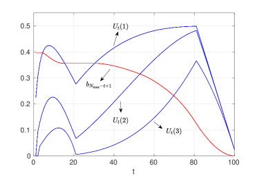
Figure 2: The graphs of sequences $\{b_{N_{\max}-t+1}\}$, $\{U_{t}(r)\}$, $t=1,2,3$ for the U-shape distribution distribution of $N$ defined in (53).

5.2.3 Expected rank minimization over random horizon

In this setting [Problem (P8) of Section 2] we would like to minimize the expected absolute rank on the event that the stopping occurs before $N$; otherwise we receive the absolute rank of the last available observation, $A_{N,N}=R_{N}$. Formally, the corresponding stopping problem is

$$V_{*}(N_{\max}) := \min_{\tau\in{\mathscr{T}}({\mathscr{R}})}\mathrm{E}\big{[}A_{\tau,N}{\bf 1}\{N\geq\tau\}+R_{N}{\bf 1}\{N<\tau\}\big{]}$$

$$= -\max_{\tau\in{\mathscr{T}}({\mathscr{R}})}\mathrm{E}\big{[}(R_{N}-A_{\tau,N}){\bf 1}\{N\geq\tau\}-R_{N}]$$

$$= -\max_{\tau\in{\mathscr{T}}({\mathscr{R}})}\mathrm{E}\big{[}(R_{N}-A_{\tau,N}){\bf 1}\{N\geq\tau\}]+\frac{1}{2}(1+\mathrm{E}N).$$

Thus, letting $q(A_{t,k})=R_{k}-A_{t,k}$ for $t\leq k$ we note that

$$I_{t,k}(r)=\mathrm{E}\big{[}q(A_{t,k})\,|\,R_{1}=r_{1},\ldots,R_{t-1}=r_{t-1},R_{t}=r\big{]}=\frac{1}{2}(k+1)-\frac{k+1}{t+1}r$$

and therefore

$$U_{t}(r)=J_{t}(r)=\sum_{k=t}^{N_{\max}}\gamma_{k}I_{t,k}(r)=\Big{(}\frac{1}{2}-\frac{r}{t+1}\Big{)}\sum_{k=t}^{N_{\max}}(k+1)\gamma_{k}.$$

If $N_{\max}=\infty$ then we require that $\mathrm{E}N<\infty$; this ensures condition (17).

In this setting $\nu=N_{\max}$ or $\nu=\tilde{N}_{\max}$ depending on support of the distribution of $N$, and

$$y_{t}(j)=\Big{(}\frac{1}{2}-\frac{j}{t+1}\Big{)}\sum_{k=t}^{\nu}(k+1)\gamma_{k},\;\;\;f_{t}(j)=\frac{1}{t},\;\;\;j=1,\ldots,t,\;\;\;t=1,\ldots,\nu.$$

The recursion for computation of the optimal value is obtained by substitution of these formulas in (32): $b_{1}=-\infty$, $b_{2}=0$, and for $t=2,\ldots,\nu$

$$b_{t+1} = \frac{1}{\nu-t+1}\sum_{j=1}^{\nu-t+1}\bigg{[}b_{t}\,\vee\,\Big{(}\frac{1}{2}-\frac{j}{\nu-t+2}\Big{)}\sum_{k=\nu-t+1}^{\nu}(k+1)\gamma_{k}\bigg{]}.$$ (54)

$$= b_{t}+\frac{1}{\nu-t+1}\sum_{j=1}^{\nu-t+1}\bigg{[}\Big{(}\frac{1}{2}-\frac{j}{\nu-t+2}\Big{)}\sum_{k=\nu-t+1}^{\nu}(k+1)\gamma_{k}-b_{t}\bigg{]}_{+}~{}.$$

The optimal policy is to stop at time $t$ if $Y_{t}=U_{t}(R_{t})>b_{\nu-t+1}$, i.e.,

$$\tau_{\ast}=\min\;\bigg{\{}t=1,\ldots,\nu:\Big{(}\frac{1}{2}-\frac{R_{t}}{t+1}\Big{)}\sum_{k=\nu-t+1}^{\nu}(k+1)\gamma_{k}>b_{\nu-t+1}\bigg{\}}.$$

Note that $V_{*}(N_{\max})=b_{N_{\max}+1}+\frac{1}{2}(1+\mathrm{E}N)$.

Gianini-Pettitt considered distributions of $N$ with finite right endpoint $N_{\max}$ and studied asymptotic behavior of the optimal value $V_{*}(N_{\max})$ as $N_{\max}\to\infty$. In particular, for distributions satisfying $\mathrm{P}(N=k|N\geq k)=(N_{\max}-k+1)^{-\alpha}$, $k=1,\ldots,N_{\max}$, $N_{\max}=1,2,\ldots$ with $\alpha>0$ one has: (a) if $\alpha<2$ then $V_{*}(N_{\max})\to\infty$ as $N_{\max}\to\infty$; (b) if $\alpha>2$ then $\lim_{N_{\max}\to\infty}V_{*}(N_{\max})=3.86945\ldots$; (c) if $\alpha=2$ then $\limsup_{N_{\max}\to\infty}V_{*}(N_{\max})$ is finite and greater than $3.86945\ldots$. Thus, if $\alpha>2$ then the optimal value $V_{*}(N_{\max})$ coincides asymptotically with the one in the classical problem of minimizing the expected rank studied in chow; see Problem (P4) in Section 2. On the other hand, if $N$ is uniformly distributed on $\{1,\ldots,N_{\max}\}$, i.e. $\alpha=1$, then $V_{*}(N_{\max})\to\infty$ as $N_{\max}\to\infty$.

We illustrate these results in Table 6. The first row of the table, $\alpha=1$, corresponds to the uniform distribution where $\gamma_{k}=1/N_{\max}$, $k=1,\ldots,N_{\max}$, while for general $\alpha>0$

$$\gamma_{k}=\frac{1}{(N_{\max}-k+1)^{\alpha}}\prod_{j=1}^{k-1}\bigg{[}1-\frac{1}{(N_{\max}-j+1)^{\alpha}}\bigg{]},\;\;\;k=1,\ldots,N_{\max};$$

see Gianini-Pettitt.

$N_{\max}$	100	500	$10^{3}$	$10^{4}$	$10^{5}$	$10^{6}$
$\alpha=1$	4.74437	8.42697	10.70615	23.34298	50.43062	108.71663
$\alpha=2$	3.83593	4.14133	4.18918	4.23792	4.24381	4.24444
$\alpha=3$	3.61069	3.80588	3.83549	3.86542	3.86909	3.86947

Table 6: Optimal values $V_{*}(N_{\max})$ computed using (54).

It is seen from the table that in the case $\alpha=3$ the optimal value approaches the universal limit of chow as $N_{\max}$ goes to infinity. For $\alpha=2$ the formula (54) yields the optimal value $4.2444\ldots$; this complements the result of Gianini-Pettitt on boundedness of the optimal value.

5.3 Multiple choice problems

The existing literature treats sequential multiple choice problems as problems of multiple stopping. However, if the reward function has an additive structure, and the involved random variables are independent then these problems can be reformulated in terms of the sequential assignment problem of Section 3. Under these circumstances the results of DLR are directly applicable and can be used in order to construct optimal selection rules. We illustrate this approach in the next two examples.

5.3.1 Maximizing the probability of selecting the best observation with $k$ choices

This setting was first considered by GiMo, and it is discussed in Section 2 as Problem (P9). The goal is to maximize the probability for selecting the best observation with $k$ choices, i.e., to maximize

$$\mathrm{P}\big{\{}\cup_{j=1}^{k}(A_{\tau_{j},n}=1)\big{\}}=\sum_{j=1}^{k}\mathrm{P}(A_{\tau_{j},n}=1)$$

with respect to the stopping times $\tau^{(k)}=(\tau_{1},\ldots,\tau_{k})$, $\tau_{1}<\cdots<\tau_{k}$ of the filtration ${\mathscr{R}}$. This problem is equivalent to the following version of the sequential assignment problem (AP1) [see Section 3].

Let $0=p_{1}=\cdots=p_{n-k}<p_{n-k+1}=\cdots=p_{n}=1$, and let

$$Y_{t}=\frac{t}{n}{\bf 1}\{R_{t}=1\},\;\;t=1,\ldots,n.$$

The goal is to maximize $S(\pi)=\mathrm{E}\sum_{t=1}^{n}p_{\pi_{t}}Y_{t}$ with respect to $\pi\in\Pi({\mathscr{Y}})$, where $\Pi({\mathscr{Y}})$ is the set of all non–anticipating policies of filtration ${\mathscr{Y}}$, i.e., $\{\pi_{t}=j\}\in{\mathscr{Y}}_{t}$ for all $j=1,\ldots,n$ and $t=1,\ldots,n$.

The relationship between sequential assignment and multiple choice problems is evident: if a policy $\pi$ assigns $p_{\pi_{t}}=1$ to the observation $Y_{t}$ then the corresponding $t$th observation is selected, i.e., events $\{p_{\pi_{t}}=1\}$ and $\cup_{j=1}^{k}\{\tau_{j}=t\}$ are equivalent.

The optimal policy for the above assignment problem is characterized by Theorem 1. Specifically, for $t=1,\ldots,n$ let $p_{t_{1}}\leq p_{t_{2}}\leq\cdots\leq p_{t_{n-t+1}}$ be the subset of the coefficients $\{p_{1},\ldots,p_{n}\}$ that are left unassigned at time $t$. Let $s_{t}=\sum_{i=1}^{n-t+1}p_{t_{i}}$ denote the number of observations to be selected (unassigned coefficients $p$’s equal to $1$). The optimal policy $\pi_{*}$ at time $t$ partitions the real line by numbers

$$-\infty=a_{0,n-t+1}\leq a_{1,n-t+1}\leq\cdots\leq a_{n-t,n-t+1}\leq a_{n-t+1,n-t+1}=\infty,$$

and prescribes to select the $t$th observation if $Y_{t}>a_{n-t+1-s_{t},n-t+1}$. In words, the last inequality means that the observation is selected if $Y_{t}$ is greater than the $s_{t}$-th largest number among the numbers $a_{1,n-t+1},a_{2,n-t+1},\ldots,a_{n-t,n-t+1}$. These numbers are given by the following formulas: $a_{0,n-t+1}=-\infty$, $a_{n-t+1,n-t+1}=\infty$, and for $j=1,\ldots,n-t$

$$a_{j,n-t+1}=\int_{a_{j-1,n-t}}^{a_{j,n-t}}z\mathrm{d}F_{t+1}(z)+a_{j-1,n-t}F_{t+1}(a_{j-1,n-t})+a_{j,n-t}(1-F_{t+1}(a_{j,n-t})),$$

where $F_{t}$ is the distribution function of $Y_{t}$. The optimal value of the problem is

$$S_{*}(k)=S(\pi_{*};k)=\sum_{j=1}^{k}a_{n-j+1,n+1}~{}.$$ (55)

In our case $F_{t}(z)=(1-\frac{1}{t}){\bf 1}(z\geq 0)+\frac{1}{t}{\bf 1}(z\geq\frac{t}{n})$, $t=1,\ldots,n$ which yields

$$a_{j,n-t+1} = \tfrac{1}{n}{\bf 1}\big{(}a_{j-1,n-t}<\tfrac{t+1}{n}\leq a_{j,n-t}\big{)}$$

$$\;+\;a_{j-1,n-t}\big{[}\big{(}1-\tfrac{1}{t+1}\big{)}{\bf 1}(a_{j-1,n-t}\geq 0)+\tfrac{1}{t+1}{\bf 1}\big{(}a_{j-1,n-t}\geq\tfrac{t+1}{n}\big{)}\big{]}$$

$$\;+\;a_{j,n-t}\big{[}\big{(}1-\tfrac{1}{t+1}\big{)}{\bf 1}(a_{j,n-t}<0)+\tfrac{1}{t+1}{\bf 1}\big{(}a_{j,n-t}<\tfrac{t+1}{n}\big{)}\big{]}$$

for $j=1,\ldots,n-t$, $a_{0,n-t+1}=-\infty$, $a_{n-t+1,n-t+1}=\infty$, and by convention we set $-\infty\cdot 0=\infty\cdot 0=0$.

Table 7 gives optimal values $S_{*}(k)$ for $n=10^{4}$ and different $k$. Note that the case $k=1$ corresponds to the classical secretary problem. It is clearly seen that the optimal probability of selecting the best observtation grows fast with the number of possible choices $k$. The numbers presented in the table agree with those given in Table 4 of GiMo.

$k$	1	2	3	4	5	6	7	8	25
$S_{*}(k)$	0.36791	0.59106	0.73217	0.82319	0.88263	0.92175	0.94767	0.96491	0.999997

Table 7: Optimal values $S_{*}(k)$ in the problem of maximizing the probability of selecting the best option with $k$ choices. The table is computed using (5.3.1) and (55) for $n=10^{4}$.

The structure of the optimal policy allows to compute distribution of the time required for the subset selection. As an illustration, we consider computation of the expected time required for selecting two options ($k=2$). According to the optimal policy the first choice is made at time $\tau_{1}:=\min\{t=1,\ldots,n:Y_{t}>a_{n-t-1,n-t+1}\}$, while the second choice occurs at time $\tau_{2}:=\min\{t>\tau_{1}:Y_{t}>a_{n-t,n-t+1}\}$. Then the expected time to the subset selection is

$$\mathrm{E}\tau_{2} = \mathrm{E}\tau_{1}+\mathrm{E}(\tau_{2}-\tau_{1}),$$ (57)

where

$$\mathrm{E}\tau_{1}=1+\sum_{j=1}^{n-1}\prod_{t=1}^{j}F_{t}(a_{n-t-1,n-1+1})$$ (58)

$$\mathrm{E}(\tau_{2}-\tau_{1})=1+\sum_{i=1}^{n-2}\mathrm{P}(\tau_{2}-\tau_{1}>i)=1+\sum_{j=1}^{n-1}\sum_{i=1}^{n-j-1}\mathrm{P}(\tau_{2}-\tau_{1}>i\,|\,\tau_{1}=j)\mathrm{P}(\tau_{1}=j)$$

$$=1+\sum_{j=1}^{n-1}\sum_{i=1}^{n-j-1}\prod_{t=1}^{j+i}F_{t}(a_{n-t,n-1+1})\mathrm{P}(\tau_{1}=j)$$

$$=1+\sum_{j=1}^{n-1}\sum_{i=1}^{n-j-1}\prod_{t=j+1}^{j+i}F_{t}(a_{n-t,n-1+1})\big{[}1-F_{j}(a_{n-j-1,n-j+1})\big{]}\prod_{t=1}^{j-1}F_{t}(a_{n-t-1,n-t+1}).$$ (59)

These formulas are clearly computationally amenable and easy to code on a computer.

5.3.2 Minimization of the expected average rank with $k$ choices

In this problem that it is discussed in Section 2 as Problem (P10) we want to minimize the expected average rank of the $k$ selected observations:

$$\min_{\tau^{(k)}}\mathrm{E}\bigg{(}\frac{1}{k}\sum_{j=1}^{k}A_{\tau_{j},n}\bigg{)},$$

where $\tau^{(k)}=(\tau_{1},\ldots,\tau_{k})$, $\tau_{1}<\cdots<\tau_{k}$ are stopping times of filtration ${\mathscr{R}}$.

This setting is equivalent to the following sequential assignment problem.

Let $0=p_{1}=\cdots=p_{n-k}<p_{n-k+1}=\cdots=p_{n}=1$, and let

$$Y_{t}=-\frac{n+1}{t+1}R_{t},\;\;t=1,\ldots,n.$$

The goal is to maximize $S(\pi)=\mathrm{E}\sum_{t=1}^{n}p_{\pi_{t}}Y_{t}$ with respect to $\pi\in\Pi({\mathscr{Y}})$.

Note that here $F_{t}$ is a discrete distribution with atoms at $y_{t}(\ell)=-\frac{n+1}{t+1}\ell$, $\ell=1,\ldots,t$ and corresponding probabilities $f_{t}(\ell):=\mathrm{P}\{Y_{t}=y_{t}(\ell)\}=\frac{1}{t}$. The structure of the optimal policy is exactly as in the previous section: at time $t$ the real line is partitioned by real numbers $a_{j,n-t+1}$, $j=0,\ldots,n-t+1$ and $t$th option if $Y_{t}>a_{n-t+1-s_{t},n-t+1}$, where $s_{t}$ stands for the number of coefficients $p_{i}$ equal to $1$ at time $t$. The constants $\{a_{j,n-t+1}\}$ are determined by the following formulas: $a_{0,n-t+1}=-\infty$, $a_{n-t+1,n-t+1}=\infty$, and for $j=2,\ldots,n-t$

$$a_{j,n-t+1} = \frac{1}{t+1}\sum_{\ell=1}^{t+1}y_{t+1}(\ell){\bf 1}\big{\{}y_{t+1}(\ell)\in(a_{j-1,n-t},a_{j,n-t}]\big{\}}$$

$$\;+\;\frac{a_{j-1,n-t}}{t+1}\sum_{\ell=1}^{t+1}{\bf 1}\big{\{}y_{t+1}(\ell)\leq a_{j-1,n-t}\big{\}}\;+\;\frac{a_{j,n-t}}{t+1}\sum_{\ell=1}^{t+1}{\bf 1}\big{\{}y_{t+1}(\ell)>a_{j,n-t}\big{\}}~{}.$$

The optimal value $S_{*}(k)$ of the problem is again given by (55). Table 8 presents $S_{*}(k)$ for $n=10^{5}$ and different values of $k$. It worth noting that $k=1$ corresponds to the standard problem of expected rank minimization [Problem (P4)] with well known asymptotics $S_{*}(k)\approx 3.8695\ldots$ as $n$ goes to infinity. Using formulas (57), (58) and (59) we also computed expected time required for $k=2$ selections when $n=10^{3}$: $\mathrm{E}\tau_{1}\approx 396.25983$ and $\mathrm{E}\tau_{2}\approx 610.54822$. Such performance metrics were not established so far and our approach illustrates the simplicity with which this can be done.

$k$	1	2	3	4	5	6	7	8	25
$S_{*}(k)$	3.86488	4.50590	5.12243	5.72330	6.31262	6.89285	7.46574	8.03255	17.22753

Table 8: The optimal value $S_{*}(k)$ in the problem of minimization of the expected average rank with $k$ choices for $n=10^{5}$.

5.4 Miscellaneous problems

The next two examples illustrate applicability of the proposed framework to some other problems of optimal stopping.

5.4.1 Moser’s problem with random horizon

This is Problem (P11) of Section 2. The stopping problem is

$$V_{*}(N_{\max}):=\max_{\tau\in{\mathscr{T}}({\mathscr{X}})}\mathrm{E}[(X_{\tau}-X_{N}){\bf 1}\{\tau\leq N\}]+\mu.$$

Define $Y_{t}=\mathrm{E}\big{[}(X_{t}-X_{N}){\bf 1}\{t\leq N\}\,|\,{\mathscr{X}}_{t}]$; then

$$Y_{t}=\sum_{k=t}^{N_{\max}}\mathrm{E}\big{[}(X_{t}-X_{N}){\bf 1}\{N=k\}\,|\,{\mathscr{X}}_{t}\big{]}=(X_{t}-\mu)\sum_{k=t}^{N_{\max}}\gamma_{k},$$

and for any stopping time $\tau\in{\mathscr{T}}({\mathscr{X}})$

$$\mathrm{E}\big{[}(X_{\tau}-X_{N}){\bf 1}\{\tau\leq N\}\big{]}=\sum_{t=1}^{\infty}\mathrm{E}\Big{[}{\bf 1}\{\tau=t\}\mathrm{E}\big{\{}(X_{t}-X_{N}){\bf 1}\{t\leq N\}\,|\,{\mathscr{X}}_{t}\big{\}}\Big{]}=\mathrm{E}Y_{\tau}.$$

Thus, the original stopping problem is equivalent to the problem of stopping the sequence of independent random variables $Y_{t}=(X_{t}-\mu)\sum_{k=t}^{N_{\max}}\gamma_{k}$, $t=1,\ldots,N_{\max}$, and the optimal value is

$$V_{*}(N_{\max})=\mu+\max_{\tau\in{\mathscr{T}}({\mathscr{Y}})}\mathrm{E}Y_{\tau}.$$

The distribution of $Y_{t}$ is $F_{t}(z)=G(\mu+\frac{z}{\sigma_{t}})$, $t=1,\ldots,N_{\max}$, where $\sigma_{t}:=\sum_{k=t}^{N_{\max}}\gamma_{k}$. Then applying Corollary 1 we obtain that the optimal stopping rule is given by

$$b_{1}=-\infty,\;\;b_{2}=\mathrm{E}Y_{N_{\max}},$$

$$b_{t+1}=\int_{b_{t}}^{\infty}z\mathrm{d}F_{N_{\max}-t+1}(z)+b_{t}F_{N_{\max}-t+1}(b_{t}),\;\;\;t=2,\ldots,N_{\max},$$

$$\tau_{*}=\min\{1\leq t\leq N_{\max}:Y_{t}>b_{N_{\max}-t+1}\}.$$

In particular, if $G$ is the uniform $[0,1]$ distribution then straightforward calculation yields: $b_{2}=0$ and

$$b_{t+1}=\frac{1}{2\sigma_{N_{\max}-t+1}}\Big{(}b_{t}+\tfrac{1}{2}\sigma_{N_{\max}-t+1}\Big{)}^{2},\;\;t=2,\ldots,N_{\max}.$$

The optimal value of the problem is $V_{*}(N_{\max})=b_{N_{\max}+1}+\frac{1}{2}$.

It is worth noting that the case of $\gamma_{k}=0$ for all $k=1,\ldots,N_{\max}-1$ and $\gamma_{N_{\max}}=1$ corresponds to the original Moser’s problem with fixed horizon $N_{\max}$. In this case $\sigma_{t}=1$ for all $t$, and the above recursive relationship coincides with the one in Moser which is $E_{t+1}=\frac{1}{2}(1+E_{t}^{2})$ where $E_{t}=b_{t}+\frac{1}{2}$.

5.4.2 Bruss’ Odds–Theorem

This is the stopping problem (P12) of Section 2. In this setting we have

$$Y_{t}:=\mathrm{P}\{Z_{t}=1,Z_{t+1}=\cdots=Z_{n}=0\,|\,{\mathscr{Z}}_{t}\}=\left\{\begin{array}[]{ll}Z_{t}\prod_{k=t+1}^{n}q_{k},&t=1,\ldots,n-1,\\ Z_{t},&t=n,\end{array}\right.$$ (60)

and then

$$V_{*}:=\max_{\tau\in{\mathscr{T}}({\mathscr{Z}})}\mathrm{P}(Z_{\tau}=1,Z_{\tau+1}=\cdots=Z_{n}=0\}=\max_{\tau\in{\mathscr{T}}({\mathscr{Y}})}\mathrm{E}Y_{\tau}.$$

Thus, the original stopping problem is equivalent to stopping the sequence $\{Y_{t}\}$ which is given in (60). Note that $Y_{t}$’s are independent, and $Y_{t}$ takes two values $\prod_{k=t+1}^{n}q_{k}$ and $0$ for $t=1,\ldots,n-1$, and $1$ and $0$ for $t=n$ with respective probabilities $p_{t}$ and $q_{t}=1-p_{t}$. Therefore applying Corollary 1 we obtain that the optimal stopping rule is given by

$$\tau_{*}=\min\bigg{\{}t=1,\ldots,n:Y_{t}>b_{n-t+1}\bigg{\}},$$ (61)

where $b_{1}=-\infty$, $b_{2}=\mathrm{E}Y_{n}=p_{n}$, and for $t=2,3,\ldots,n$

$$b_{t+1} =\int_{b_{t}}^{\infty}z\mathrm{d}F_{n-t+1}(z)+b_{t}F_{n-t+1}(b_{t})=b_{t}+p_{n-t+1}\bigg{[}\prod_{k=n-t+2}^{n}q_{k}-b_{t}\bigg{]}_{+},$$ (62)

where $[\cdot]_{+}=\max\{0,\cdot\}$. The problem optimal value is $V_{*}=b_{n+1}$.

Now we demonstrate the stopping rule (61)–(62) is equivalent to the sum–odds–and–stop algorithm of Bruss. According to (61), it is optimal to stop at the first time instance $t\in\{1,\ldots,n-1\}$ such that $Z_{t}=1$ and $b_{n-t+1}(\prod_{k=t+1}^{n}q_{k})^{-1}<1$; if such $t$ does not exist then the stopping time is $n$. Note that

$$\frac{b_{n-t+1}}{\prod_{k=t+1}^{n}q_{k}}=\frac{b_{n-t}}{\prod_{k=t+1}^{n}q_{k}}+\frac{p_{t+1}}{q_{t+1}}\bigg{[}1-\frac{b_{n-t}}{\prod_{k=t+2}^{n}q_{k}}\bigg{]}_{+},\;\;t=0,1,\ldots,n-2.$$ (63)

Define $u_{s}:=b_{s}(\prod_{k=n-s+2}^{n}q_{k})^{-1}$, $s=2,\ldots,n+1$. It is evident that $\{u_{s}\}$ is a monotone increasing sequence, and with this notation (63) takes the form

$$u_{n-t+1} = \frac{1}{q_{t+1}}u_{n-t}+\frac{p_{t+1}}{q_{t+1}}(1-u_{n-t})_{+},\;\;\;t=0,1,\ldots,n-2,$$ (64)

$$u_{2} = \frac{p_{n}}{q_{n}}.$$ (65)

In terms of the sequence $\{u_{s}\}$ the optimal stopping rule (61) is the following: it is optimal to stop at first time $t\in\{1,\ldots,n-1\}$ such that $Z_{t}=1$ and $u_{n-t+1}<1$; if such $t$ does not exist then stop at time $n$. Formally, define $t_{*}:=\min\{t=1,\ldots,n-1:u_{n-t+1}<1\}$ if it exists. Then for any $t\in\{t_{*},t_{*}+1.\ldots,n-1\}$ we have $u_{n-t+1}<1$ and iterating (64)-(65) we obtain

$$u_{n-t+1}=u_{n-t}+\frac{p_{t+1}}{q_{t+1}}=\sum_{k=t+1}^{n}\frac{p_{k}}{q_{k}},\;\;\;t=t_{*},t_{*}+1,\ldots,n-1.$$ (66)

Therefore (61) can be rewritten as

$$\tau_{*}=\inf\bigg{\{}t=1,\ldots,n-1:Z_{t}=1\;\;\hbox{and}\;\;\sum_{k=t+1}^{n}\frac{p_{k}}{q_{k}}<1\bigg{\}}\wedge n,$$

where by convention $\inf\{\emptyset\}=\infty$. In order to compute the optimal value $V_{*}=b_{n+1}$ we need to determine $u_{n+1}$. For this purpose we note that the definition of $t_{*}$ and (64) imply

$$u_{n-t+1}=\frac{u_{n-t}}{q_{t+1}},\;\;\;t=t_{*}-1,t_{*}-2,\ldots,1,0,$$ (67)

and, in view of (66), $u_{n-t_{*}+1}=\sum_{k=t_{*}+1}^{n}(p_{k}/q_{k})$. Therefore iterating (67) we have

$$u_{n+1}=\bigg{(}\prod_{j=1}^{t_{*}}\frac{1}{q_{j}}\bigg{)}u_{n-t_{*}+1}=\bigg{(}\prod_{j=1}^{t_{*}}\frac{1}{q_{j}}\bigg{)}\sum_{k=t_{*}+1}^{n}\frac{p_{k}}{q_{k}}.$$

Taking into account that $u_{n+1}=b_{n+1}(\prod_{j=1}^{n}q_{j})^{-1}$ we finally obtain the optimal value of the problem:

$$V_{*}=b_{n+1}=\prod_{j=t_{*}+1}^{n}q_{j}\sum_{k=t_{*}+1}^{n}\frac{p_{k}}{q_{k}}.$$

These results coincide with the statement of Theorem 1 in Bruss.

6 Concluding remarks

We close this paper with several remarks.

1. In this paper we show that numerous problems of sequential selection can be reduced to the problem of stopping a sequence of independent random variables with carefully specified distribution functions. In terms of computational complexity, we cannot assert that in all cases our approach leads to a more efficient algorithm than a dynamic programming recursion tailored for a specific problem instance. However, in contrast to the latter, in many cases of interest we are able to derive explicit recursive relationships that can be easily implemented; see, e.g., Problem (P5) that has not been solved to date, or Problems (P6) and (P7) for which our approach provides explicit expressions for computation of optimal policies under arbitrary distribution of the horizon length. The conditioning argument leads to rules expressed in terms of “sufficient statistics”; such rules are very natural, simple, and easy to interpret.

2. The proposed framework is applicable to sequential selection problems that can be reduced to settings with independent observations and additive reward function. In addition, it is required that the number of selections to be made is fixed and does not depend on the observations. As the paper demonstrates, this class is rather broad. In particular, it includes selection problems with no-information, rank-dependent rewards and fixed or random horizon. The framework is also applicable to selection problems with full information when the random variables $\{X_{t}\}$ are observable, and the reward for stopping at time $t$ is a function of the current observation $X_{t}$ only. It is worth noting that in all these problems the optimal policy is of the memoryless threshold type. In addition, we demonstrate that multiple choice problems with fixed and random horizon and additive reward, as well as sequential assignment problems with independent job sizes and random horizon, are also covered by the proposed framework. In particular, variants of problems (P9), (P10) and (P12) with random horizon can also be solved using the proposed approach.

3. Although the approach holds for a broad class of sequential selection problems, there are settings that do not belong to the indicated class. For instance, settings with rank–dependent reward and full information as in [Section 3]GiMo and gnedin cannot be reduced to optimal stopping of a sequence of independent random variables. A prominent example of such a setting is the celebrated Robbins’ problem of minimizing the expected rank on the basis of full information. This problem is still open, and only bounds on the asymptotic optimal value are available in the literature. Remarkably, Bruss-Ferguson show that no memoryless threshold rule can be optimal in this setting, and the optimal stopping rule must depend on the entire history.

4. The proposed approach is not applicable to settings where the number of selections is not fixed and depends on the observations. This class includes problems of maximizing the number of selections subject to some constraints; for representative publications in this direction we refer, e.g., to Samuels-Steele, Coffman, Gnedin99, Arlotto15 and references therein. Another example is the multiple choice problem with zero–one reward; see, e.g., Rose and Vanderbei where the problem of maximizing the probability of selecting the $k$ best alternatives was considered. The fact that the results of DLR are not applicable to the latter problem was already observed by Rose who mentioned this explicitly.

Acknowledgement.

The authors thank two anonymous reviewers for exceptionally insightful and helpful reports that led to significant improvements in the paper. The research was supported by the grants BSF 2010466 and ISF 361/15.

References

- [1] \harvarditemAjtai et al.2001Megiddo Ajtai, M., Megiddo, N. and Waarts, O. (2001). Improved algorithms and analysis for secretary problems and generalizations. SIAM J. Discrete Math. 14, 1–27.
- [2] \harvarditemAlbright1972albright Albright, S. C., Jr. (1972). Stochastic sequential assignment problems. Technical report No. 147, Department of Statistics, Stanford University. \harvarditemArlotto & Gurvich2018Arlotto Arlotto, A. and Gurvich, I. (2018) Uniformly bounded regret in the multi-secretary problem. Stochastic Systems 9, 231–260. \harvarditemArlotto et al.2015Arlotto15 Arlotto, A., Nguyen, Vinh V. and Steele, J. M. (2015). Optimal online selection of a monotone subsequence: a central limit theorem. Stochastic Process. Appl. 125, 3596–3622. \harvarditemBerezovsky & Gnedin1984gnedin-book Berezovsky, B.A. and Gnedin, A. B. (1984). The Problem of Optimal Choice. Nauka, Moscow (in Russian).
- [3] \harvarditemBruss2000Bruss Bruss, F. T. (2000). Sum the odds and stop. Ann. Probab. 26, 1384–1391. \harvarditemBruss2019Bruss19 Bruss, F. T. (2019). Odds–theorem and monotonicity. Mathematica Applicanda 47, 25–43.
- [4] \harvarditemBruss & Louchard2016Bruss-2016 Bruss, F. T. and Louchard, G. (2016). Sequential selection of the best out of rankable objects. Discrete Math. Theor. Comput. Sci. 18, no. 3, Paper No. 13, 12 pp. \harvarditemBruss & Ferguson1996Bruss-Ferguson Bruss, F. T. and Ferguson, T. (1996). Half–prophets and Robbins’ problem of minimising the expected rank with i.i.d. random variables. Athens Conference on Applied Probability and Time Series Analysis, Vol. I (1995), 1–17, Lect. Notes Stat., 114, Springer, New York.
- [5] \harvarditemChow et al.1964chow Chow, Y. S., Moriguti, S., Robbins, H. and Samuels, S. M. (1964). Optimal selection based on relative rank (the ”Secretary problem”). Israel J. Math. 2, 81–90. \harvarditemChow et al.1971chow-rob-sieg Chow, Y. S., Robbins, H. and Siegmung, D. (1971). Great Expectations: The Theory of Optimal Stopping. Houghton Mifflin Company, Boston \harvarditemCoffman et al,1987Coffman Coffman, E. G., Jr., Flatto, L. and Weber, R. R. (1987). Optimal selection of stochastic intervals under a sum constraint. Adv. in Appl. Probab. 19, 454–473. \harvarditemDerman, Lieberman & Ross1972DLR Derman, C., Lieberman, G. J. and Ross, S. (1972). A sequential stochastic assignment problem. Management Science 18, 349–355. \harvarditemDietz et al.2011DiLaRi Dietz, C., van der Laan, D. and Ridder, A. (2011). Approximate results for a generalized secretary problem. Probab. Engrg. Inform. Sci. 25, 157-169. \harvarditemDynkin1963Dyn Dynkin, E. B. (1963). The optimum choice of the instant for stopping a Markov process. (Russian) Dokl. Akad. Nauk SSSR 150, 238-240. Also in: Selected papers of E. B. Dynkin with commentary, 485–488. Edited by A. A. Yushkevich, G. M. Seitz and A. L. Onishchik. American Mathematical Society, Providence, RI; International Press, Cambridge. \harvarditemFerguson1989ferguson Ferguson, T. S. (1989). Who solved the secretary problem? Statist. Science 4, 282–296. \harvarditemFerguson2008F2008 Ferguson, T.S. (2008). Optimal Stopping and Applications. https://www.math.ucla.edu/t̃om/Stop–ping/Contents.html \harvarditemFrank & Samuels1980FrSa Frank, A. Q. and Samuels, S. M. (1980). On an optimal stopping problem of Gusein–Zade. Stoch. Proc. Appl. 10, 299-311. \harvarditemFreeman1983freeman Freeman, P. R. (1983). The secretary problem and its extensions: a review. Int. Statist. Review 51, 189-206. \harvarditemGianini-Pettitt1979Gianini-Pettitt Gianini-Pettitt, J. (1979). Optimal selection based on relative ranks with a random number of individuals. Adv. Appl. Probab. 11, 720–736. \harvarditemGilbert and Mosteller1966GiMo Gilbert, J. and Mosteller, F. (1966). Recognizing the maximum of a sequence. J. Amer. Statist. Assoc. 61, 35-73. \harvarditemGoldenshluger and Zeevi2018GZ Goldenshluger, A. and Zeevi, A. (2018). Optimal stopping of a random sequence with unknown distribution. Preprint. \harvarditemGnedin1999Gnedin99 Gnedin, A. V. (1999). Sequential selection of an increasing subsequence from a sample of random size. J. Appl. Probab. 36, 1074–1085. \harvarditemGnedin2007gnedin Gnedin, A. V. (2007). Optimal stopping with rank-dependent loss. J. Appl. Probab. 44, 996–1011. \harvarditemGnedin & Krengel1996gnedin-krengel Gnedin, A. V. and Krengel, U. (1996). Optimal selection problems based on exchangeable trials. Ann. Appl. Probab. 6, 862–882. \harvarditemGusein–Zade1966GuZa Gusein–Zade, S. M. (1966). The problem of choice and the optimal stopping rule for a sequence of independent trials. Theory Probab. Appl. 11, 472–476. \harvarditemHaggstrom1967Haggstrom Haggstrom, G. W. (1967). Optimal sequential procedures when more than one stop is required. Ann. Math. Statist. 38, 1618–1626. \harvarditemIrle1980Irle80 Irle, A. (1980). On the best choice problem with random population size. Zeitschrift für Operations Research 24, 177–190. \harvarditemKawai & Tamaki2003KT2003 Kawai, M. and Tamaki, M. (2003). Choosing either the best or the second best when the number of applicants is random. Comput. Math. Appl. 46, 1065–1071.
- [6] \harvarditemKrieger & Samuel-Cahn2009krieger-ester Krieger, A. M. and Samuel-Cahn, E. (2009). The secretary problem of minimizing the expected rank: a simple suboptimal approach with generalizations. Adv. in Appl. Probab. 41, 1041–1058 \harvarditemKrieger et al.2007kep-aap1 Krieger, A. M., Pollak, M. and Samuel-Cahn, E. (2007). Select sets: rank and file. Ann. Appl. Probab. 17, 360–385. \harvarditemKrieger et al.2008kep-jap Krieger, A. M., Pollak, M. and Samuel-Cahn, E. (2008). Beat the mean: sequential selection by better than average rules. J. Appl. Probab. 45, 244–259.
- [7] \harvarditemLin et al.2019Yao Lin, Y.-S., Hsiau, S.-R. and Yao, Y.-C. (2019). Optimal selection of the -th best candidate. Probab. Engrg. Inform. Sci. 33, 327–347. \harvarditemLindley1961lindley Lindley, D. V. (1961). Dynamic programming and decision theory. Appl. Statist. 10, 39–51.
- [8] \harvarditemMatsui & Ano2016Matsui Matsui T. and Ano, K. (2016). Lower bounds for Bruss’ Odds Theorem with multiple stoppings. Math. Oper. Res. 41, 700–714.
- [9] \harvarditemMoser1956Moser Moser, L. (1956). On a problem of Cayley. Scripta Math. 22, 289–292. \harvarditemMucci1973mucci-a Mucci, A. G. (1973). Differential equations and optimal choice problems. Ann. Statist. 1, 104–113. \harvarditemNikolaev & Jacobson2010Jacobson Nikolaev, A. G. and Jacobson, S. H. (2010). Stochastic sequential decision–making with a random number of jobs. Oper. Res. 58, 1023–1027. \harvarditemNikolaev & Sofronov2007Nikolaev-Sofronov Nikolaev, M. L. and Sofronov, G. (2007). A multiple optimal stopping rule for sums of independent random variables. Discrete Math. Appl. 17, 463–473. \harvarditemPresman and Sonin1972PS1972 Presman, E. L. and Sonin, I. M. (1972). The best choice problem for a random number of objects. Teor. Veroyatnost. i Primenen. 17, 695-706. \harvarditemQuine & Law1996QuLaw Quine, M. P. and Law, J. S. (1996). Exact results for a secretary problem. J. Appl. Probab. 33, 630–639. \harvarditemRobbins1970robbins70 Robbins, H. (1970). Optimal stopping. Amer. Math. Monthly 77, 333-343.
- [10] \harvarditemRobbins1991Robbins-91 Robbins, H. (1991). Remarks on the secretary problem. Amer. J. Math. and Management Sci. 11, 25–37. \harvarditemRose1982aRose Rose, J.S (1982a). A problem of optimal choice and assignment. Oper. Res. 30, 172-181. \harvarditemRose1982bRose-2 Rose, J.S. (1982b). Selection of nonextremal candidates from a sequence. J. Optimization Theory Applic. 38, 207-219. \harvarditemSakaguchi1984sakaguchi Sakaguchi, M. (1984). A sequential stochastic assignment problem with an unknown number of jobs. Math. Japonica 29, 141–152. \harvarditemSamuels1991samuels Samuels, S. (1991). Secretary problems. In: Handbook of Sequential Analysis edited by B. K. Ghosh and P.K.Sen. Marcel Dekker Inc., New York. \harvarditemSamuels & Steele1981Samuels-Steele Samuels, S. M. and Steele, J. M. (1981). Optimal sequential selection of a monotone sequence from a random sample. Ann. Probab. 9, 937–947.
- [11] \harvarditemSzajowski1982Szajowski1982 Szajowski, K. (1982). Optimal choice of an object with th rank (Polish). Mat. Stos. 19, 51-65.
- [12] \harvarditemWoryna2017Woryna2017 Woryna, A. (2017). The solution of a generalized secretary problem via analytic expressions. J. Comb. Optim. 33, 1469-1491.
- [13] \harvarditemVanderbei1980Vanderbei Vanderbei, R.J. (1980). The optimal choice of a subset of a population. Math. Oper. Res. 5, 481-486. \harvarditemVanderbei2012Vanderbei2012 Vanderbei, R.J. (2012). The postdoc variant of the secretary problem. Tech. Report. \harvarditemYeo1997yeo Yeo, G. F. (1997). Duration of a secretary problem. J. Appl. Probab. 34, 556-558.
- [14]