XEFT, the challenging path up the hill: and
Abstract
There is increasing need to assess the impact and the interpretation of and operators within the context of the Standard Model Effective Field Theory (SMEFT). The observational and mathematical consistency of a construct based on and operators is critically examined in the light of known theoretical results. The discussion is based on a general theory and its effective extension, XEFT; it includes elimination of redundant operators and their higher order compensation, SMEFT in comparison with ultraviolet completions incorporating a proliferation of scalar and mixings, canonical normalization of effective field theories, gauge invariance and gauge fixing, role of tadpoles when constructing XEFT at NLO, heavy-light contributions to the low energy limit of theories containing bosons and fermions, one-loop matching, EFT fits and their interpretation and effective field theory interpretation of derivative-coupled field theories.
keywords:
Effective Field TheoriesPACS:
11.10.Gh , 11.10.Lm , 11.15.Bt1 Introduction
Consider a four-dimensional theory, , described by a Lagrangian with a symmetry group : the goal of this work is to critically discuss some of the issues related to the construction of its “effective” extension; the XEFT extension will be described by a Lagrangian
| (1) |
where is the cutoff of the effective theory, are Wilson coefficients and are -invariant operators of mass-dimension involving the fields. The definition of EFT extension requires a more detailed description for which we need to consider , the ultraviolet (UV) completion of or the next theory in a tower of theories, . A related point to consider: is the leading order approximation of but a strictly renormalizable has no encoded information about the scale at which it stops being a meaningful representation of a complete theory. There are two possibilities in going from to :
-
a)
is based on but contains heavy degrees of freedom belonging to some representation of or
-
b)
is based on a larger group where should contain and should reduce to at low energies.
An additional assumption is that there are no “undiscovered” degrees of freedom in that are light and weakly coupled. More broadly, one generally excludes light particles, neutral under , that interact with the particles only through the exchange of new heavy particles. When is the standard model (SM) and the most simple examples in category a) are the SM singlet extension and the THDMs, containing two scalar doublets, see Ref. [1] for a review. In category b) an example is given by a non supersymmetric [2] which breaks down to the SM through a chain of different intermediate groups. Another example is , the so-called model [3]. The Lagrangian of Eq.(1) assumes that all the degrees of freedom should be incorporated; for the SM the EFTs are further distinguished by the presence of a Higgs doublet (or not) in the construction, see Ref. [4] for a review. In the SMEFT the EFT is constructed with an explicit Higgs doublet, while in the HEFT (an Electroweak chiral Lagrangian with a dominantly scalar) no such doublet is included.
In the rest of this paper we discuss several issues that arise in constructing an EFT (up to and including operators), i.e. using XEFT context, we derive several results that are relevant to the challenges presented to present and future theorists and experimentalists working to go beyond the SM:
-
①
The traditional way of using an EFT is based on matching the EFT to the full theory in order to reproduce the correct matrix elements, i.e. we choose the coefficients to be those appropriate for the full theory. After the Higgs boson discovery we have a paradigm shift, i.e. we use the EFT for fitting the data; at this point the “fitted” Wilson coefficients are the pseudo-data and we take a specific BSM model, compute the corresponding low-energy limit and choose the BSM parameters to be those appropriate for the pseudo-data.
-
②
SMEFT assumes a Higgs doublet, so any mixing among scalars (in general among heavy and light degrees of freedom) in the high-energy theory brings us to the HEFT/SMEFT dichotomy. Although there is a wide class of BSM models that support the linear SMEFT description, this realization does not always provide the appropriate framework.
-
③
When looking at fitting the data and interpreting the results, several steps should be kept in mind. Fitting requires a basis, something that everyone agrees on using, but any XEFT description truncated at level depends on many choices; in particular a “ -quadratic” description can be defined in many ways (for instance by taking into account canonical normalization of the Lagrangian, scheme dependence in the renormalization procedure or double insertion of operators), not only by the inclusion of terms. A basis is defined by eliminating redundant operators through field redefinitions (akas, equation of motion), however the equivalence of two operators is a property of XEFT while it is possible for the theory to generate one but not the other; so, in short, we may need to replace an operator involving a field (appearing in the XEFT basis) with an operator not involving that field (appearing in the low energy limit of ). Interpreting the fits requires to translate the experimental bounds on the Wilson coefficients in one basis (the XEFT basis) into limits on coefficients in another basis, the latter being computable functions of the parameters of . This requires our ability to change basis, a correspondence which is linear only at level.
-
④
Details regarding the introduction of heavy-light contributions from to XEFT are also important and explicit results are provided that highlight why they should not be ignored. Consider the set of one-loop diagrams in the theory with light external legs: some of them contain heavy and light internal lines and, after computing the low energy limit, produce non-local terms which are in correspondence with XEFT computed at one loop. It is crucial to note that non-local terms (e.g. kinematic logarithms) arise from diagrams of the underlying theory showing normal thresholds in the low-energy region. In this way one obtains comprehensive results showing the downside of neglecting XEFT at one-loop, which should be seen as the leading term in the Mellin-Barnes expansion of . Heavy-light terms describe a multi scale scenario: the light masses, the Mandelstam invariants characterizing the process and the heavy scale .
-
⑤
It is now generally accepted that a convenient formulation of SMEFT requires the so-called “canonical normalization” which should be understood to mean “proper normalization of the sources entering the -matrix”. This procedure calls into question how we perform “gauge fixing” and how “gauge invariance” is preserved. We can simultaneously redefine couplings, mixing angles and masses so that the part of the XEFT Lagrangian which is quadratic in the fields has the same functional form of the original Lagrangian but with transformed fields and parameters. This redefinition will change how we set the parameters input.
The paper is organized as follows. section 2 introduces the problem. In section 3 we discuss EoMs. In section 4 – section 6 we analyze different types of EFTs, from a simple theory containing one, real, scalar field to SMEFT. The question of redundancy is discussed and other relevant issues are examined, e.g. canonical normalization of the EFT, mixing among scalars in , gauge invariance after canonical normalization, gauge fixing. In section 7 – section 9 we study the so-called heavy-light effects when going from to XEFT and also their interplay with the NLO extension [5] of XEFT. A final issue concerns operators belonging to the class and the interpretation of derivative-coupled field theories that we discuss in section 10. Our conclusions are drawn in the final section.
2 General aspects of XEFT
In this section we give a summary of the main ingredients which are needed to study weakly interacting modifications of the Higgs sector and the electroweak gauge sector of the SM.
The heavy scale
The choice of 111For the role of in two types of empirically equivalent EFTs, Wilsonian EFTs and continuum EFTs see Ref. [6]. in Eq.(1) is crucial when going from to ; more details on this topic can be found in Refs. [7, 8, 9]. For instance, in any BSM model (e.g. the singlet extension of the SM) the scale should not be confused with the mass of the heavy Higgs boson (or with masses of new particles) – it is generally a ratio of mass and powers of couplings. It is also relevant to observe that the low energy behavior of should be computed in the mass eigenbasis, not in the weak eigenbasis.
Mixing
The important point to stress is that the EFT extension of , as defined in Eq.(1), requires absence of mixing between heavy and light degrees of freedom. The argument is simple, consider the singlet extension of the SM (HSESM) where we have one scalar doublet and one singlet; the SM scalar field (with hypercharge ) is
| (2) |
while the singlet is . There is a mixing angle such that
| (3) |
are the mass eigenstates, one light Higgs () and one heavy Higgs ().
Mixing and gauge invariance
Of course the Lagrangian remains gauge invariant but gauge invariance of the low energy theory is more complicated since we integrate the field, and does not transform as the SM Higgs boson, see sect. of Ref. [9]. For instance alone is not invariant; of course the full is gauge invariant, but is not. If the doublet is the one in Eq.(2) we introduce
| (4) |
where is a function of the parameters of the HSESM Lagrangian. At we obtain
| (5) |
and does not transform as a doublet. The infinitesimal transformations are:
| 0 | |||||
| - | (6) |
where are the parameters of the infinitesimal transformation and is the cosine(sine) of the weak mixing angle. To write the expansion of Eq.(6) we introduce
| (7) |
and also
| (8) |
where are Pauli matrices and . At we obtain
| (9) |
Working at we can split the total Lagrangian into
| (10) |
The sum over in is due to the expansion of in terms of . After integrating out in the -dependent Lagrangian we will have a tree generated effective Lagrangian, , a loop generated one and the tadpole contributions; for instance, is not invariant under the transformation of Eq.(6) with (no mixing) but the sum of and of restores invariance at . The procedure can be iterated order-by-order, i.e. the gauge transformations may be seen as generating new vertices in the theory and gauge invariance requires that, for any Green’s function, the sum of all diagrams containing one -vertex cancel. When sources are added to the Lagrangian the field transformation generates special vertices that are used to prove equivalence of gauges and simply-contracted Ward-Slavnov-Taylor identities [10, 11, 12]. Therefore, for any “transformed” Green’s function we integrate the field and, order-by-order in (including terms due to the expansion of the mixing), terms containing one -vertex continue to cancel (and WST identities to be valid).
The crucial point is that there is a substantial difference between integrating out [13, 14] the field (as often done in the literature) or the field. The first choice overlooks the mixing but is also a function of and the limit (as well as the choice of ) should be taken consistently [9]. Furthermore, SMEFT at reproduces the effect of scalar mixing on interactions involving one light Higgs scalar, but fails otherwise [15, 16]; additionally, the difference between integrating out or is at the level of operators, i.e. of , and should not be neglected when including terms.
Examples of local operators appearing in this context are or where ( invariant) and they should not be confused with and of the the basis commonly referred to as the “Warsaw basis” [17], the latter being built with the scalar doublet.
To summarize, if is the SM and we have in mind an without mixing, then the EFT extension of the SM is what we call SMEFT. It should be clear that a geometric formulation of the so-called HEFT [18, 19, 20, 21, 22] seems the most promising road for general mixings in the scalar sector. For the developing of SMEFT and HEFT approaches, that are consistent versions of EFTs, systematically improvable with higher order corrections, see Ref. [4].
As a side note, there are other approaches where the HSESM Lagrangian is augmented with higher dimensional terms, therefore assuming a different underlying UV completion, and mixing effects are studied in this wider context [23].
Examples of extensions of the SM with general new vector bosons have been discussed in Ref. [24] where the full SM gauge symmetry has been used to classify the extra vectors, see their tab. . It is worth noting that in their classification mass mixing terms of SM and new vectors are forbidden by gauge invariance; however, there could be interactions with the Higgs doublet that give rise to mass mixing of the and bosons with the new vectors when the electroweak symmetry is broken. The case with general scalar, spinor and vector field content and arbitrary interactions can be found in Refs. [25, 26, 27, 28].
More informations on extra scalar fields and mixing are discussed in Refs. [29, 30] where the notion of (approximate) alignment is discussed. For instance, exact tree-level Higgs alignment is satisfied in the inert doublet model [31] (IDM); in the IDM, the SM Higgs boson resides entirely in one of the two scalar doublets.
The question of gauge invariance can also be illustrated by starting with the SM Lagrangian and by integrating out the massive electroweak gauge bosons, the Higgs boson, and the top quark fields. The gauge group of the resulting low-energy effective field theory (LEFT) is QCDQED [32, 33] and the photon is not the field in . Stated differently, are integrated out, not the fields.
Proliferation of scalars and mixing
The lack of discovery of beyond-the-SM (BSM) physics suggests that the SM is “isolated” [34], including small mixing between light and heavy scalars. The small mixing scenario raises the following question: if there are may scalars then we have to assume that there is at least the same small mixing for every one of them. This is no longer accidental but systematic, and so must involve a principle, such as a symmetry or some other restriction to the theory that enforces the small mixing. This principle is unknown, see Ref. [35] for a detailed discussion.
Bases, over-complete sets
We now return to the XEFT defined by Eq.(1), in particular SMEFT; the main emphasis will be on consistency of the theory and not on phenomenological applications. Buildind any XEFT means promoting a theory with a finite number of terms into an effective field theory with an infinite number of terms and it is important to establish its consistency, both observational and mathematical consistency. Let us return to the “infinite number of terms”: including every operator allowed by gives over-complete sets of -dimensional operators, the well-known problem of redundancy.
Given two operators, and the set is over-complete if all elements of the -matrix depend on one linear combination of and .
Removal of redundant operators
There are several sources of degeneracy, operators differing for a total derivative (IPB), operators related by Fierz identities, Bianchi identities etc. Finally, we have the so-called EoM (equation of motion) degeneracy 222General aspects of EoM for EFTs have been discussed in Refs. [36, 37].; usually we find statements like “by using EoM we can remove ”, meaning that many linear combinations of operators “vanish by the Equations of Motion”. The original analysis of operators can be found in Ref. [38]; the question of redundancy has been initiated in Ref. [17], the so-called Warsaw basis, and continued in Refs. [39, 40, 41, 42, 43, 44, 45, 46, 47, 48, 49]. Extension to with the introduction of novel techniques (Hilbert series) can be found in Refs. [50, 51, 52, 53, 54]. If one is interested in the basis then the necessary EoMs are going to be used at , i.e. we can derive them from alone. This last statement, taken out of context, creates the impression that the basis requires EoMs used naively at ; more details will be given in subsection 4.1.
To summarize: we can remove redundant operators directly in the Lagrangian, instead of having the “cancellation” occur when the -matrix element is constructed. To some extent we can compare this removal to the use of the ’t Hooft-Feynman gauge instead of the more general gauge; since we know that the -matrix elements do not depend on the calculation is more conveniently performed by starting with . On the other hand, keeping an arbitrary provides a powerful check on the final result. It has been pointed out in Ref. [55] that, even if the -matrix elements cannot distinguish between two equivalent operators and , there is a large quantitative difference whether the underlying theory can generate or not. It is equally reasonable not to eliminate redundant operators and, eventually, exploit redundancy to check -matrix elements. In any case, redundancy means that we can only “measure” , where are Wilson coefficients. Selecting or defines different bases, i.e. the equivalence relation can be used to partition operators into equivalence classes, from which basis operators are selected.
PTG and LG
Additional selection criteria have been introduced in Ref. [45], particularly that a basis should be chosen from among Potentially-Tree-Generated (PTG) operators (as compared to LG, Loop-Generated operators). In Ref. [45] it is shown that the SM Warsaw basis [30] for operators satisfies this criterion. Note that suppressing operators containing field strengths by loop factors was shown to not be a model independent EFT statement in Ref. [56]. However, it has been pointed out that the classes of operators generated at a given loop level do not form a vector subspace, in general [57]. The appearance of an holomorphic structure has been discussed in Refs. [58, 59].
There is more: the introduction of “phenomenological truncation” will introduce ambiguities [57, 48]. For instance, given a basis of operators one could then try to truncate by retaining only operators featuring a limited set of fields, , in that basis. But such a truncation certainly does not correspond to the class of theories with new physics in . If we change to a basis in which we replace an operator involving a field with an operator not involving that field, then the truncated space of physical operators that we obtain will also change.
In section 3 we will review the notion of higher order compensation of a -dimensional redundant operator. Here we need only recall that removing a redundant operator with a Wilson coefficient will propagate into the Wilson coefficients of operators. In the bottom-up approach it does not matter since we only “measure” combinations of Wilson coefficients, linear in the coefficients and quadratic in . Indeed, when constructing the original EFT, one must include all possible operators consistent with the symmetries at every order in the expansion. Thus, the shift due to the field redefinition can be absorbed into the coefficients of operators that are already present in the theory. However, the low energy limit of the underlying theory may contain some as well as some whose compensations contain ; the Wilson coefficient is now computable in terms of the parameters of the underlying theory but what we “measure” at low energy is not .
In the previous argument and for the sake of simplicity we have neglected the mixing among Wilson coefficients: in dimensional regularization, the UV divergences are of the form ; after introducing counterterms the finite part of the coefficient is fixed by matching (NLO) while the coefficient of the logarithm is the anomalous dimension of the operator coefficient, telling us how the coefficient runs with scale. Not only do operator coefficients “run”, like couplings, they can also“mix” into each other. This is true for renormalizable, or not, theories; if the underlying theory is not known, the effective theory still has to be renormalized and infinities absorbed in the various couplings or Wilson coefficients [60]. Of course, the great advantage of (strictly) renormalizable theories, is that there are a finite number of terms in the Lagrangian.
What we are discussing here should not be confused with the fact that one can constrain from data in the SMEFT without reference to any ultraviolet (UV) completion, i.e. we can certainly treat SMEFT as a real field theory [5, 61]. One practical question that needs to be asked is whether or not the results of a fit can be translated into weakly interacting extensions of the SM. Here many of the theoretical issues (can the language of higher-dimensional Lagrangians be efficiently linked to the structure of ultraviolet completions of the SM gauge and Higgs sectors?) cannot be separated from experimental uncertainties. To sum up:
-
①
We want to study weakly interacting modifications of the Higgs sector and the electroweak gauge sector of the SM.
-
②
For each of these models we construct the and Lagrangians, compute LHC observables and EWPD, and compare the predictions from this Lagrangian and from the full model.
-
③
The important point is that for our classes of models we can derive the structure of the Wilson coefficients. To give examples we mention Refs. [62, 63] and Ref. [64] which introduces an exactly solvable large model which reduces at low energies to the SM plus the dimension six Higgs-gauge operators that are classified as and in Ref. [30]; the corresponding Wilson coefficients are given in Eqs. of Ref. [64]. Can we derive the size of the Wilson coefficients from the fits? Stated differently [65], can we interpret precision measurements as constraints on a given UV model? If we can make quantitative statements then the question of higher order compensation of redundant operators becomes relevant.
3 Equation of Motion
Although well-known in the literature (it has been explicitly emphasized in Refs. [66, 54]), let us summarize what is meant by “using EoM”. Consider a Lagrangian containing one real scalar field,
| (11) |
If we perform the transformation
| (12) |
the Lagrangian transforms as , with
| (13) | |||||
The term of second order in the derivatives cancels in the transformed Lagrangian and the -matrix remains unchanged. For a discussion on the Jacobian of the transformation and the inclusion of a source term see Refs. [67, 68]. Therefore, “using EoMs” means that the redundant operators are of the form
| (14) |
Note that we have neglected higher order terms since the goal was constructing the Lagrangian. Of course one could work at second order in , including operators, etc.. The result is
| (15) |
As a side note, there is a diagrammatic proof of these relations, see sect. of Ref. [69]. Normally we have , where is a polynomial in and the redundant operator is
| (16) |
Of course it would be simpler to replace everywhere with but this is only consistent at , i.e. neglecting terms.
When XEFT is SMEFT and the group is we construct according to the work of Ref. [17], obtaining the so-called Warsaw basis. The extension to higher dimensional bases is better performed using the tool known as Hilbert series [52, 53, 54], where the output of the Hilbert series is the number of invariants at each mass dimension, and the field content of the invariants. One can find in Ref. [70] a translation of the output of the Hilbert series for SMEFT into a format that is useful for calculating Feynman rules. Therefore, in Ref. [70] one can find a form of where all redundant operators have been removed, after assuming that is taken from Ref. [17].
We conclude re-emphasizing that, in fact, the effective field theory can be rewritten by freely using the naive classical EOM (i.e. without gauge-fixing and ghost terms) derived from , provided one considers only on-shell matrix elements at first order in . In particular, the effective Lagrangian may be reduced by the EOM before (RG improved) short-distance corrections are evaluated.
In the rest of the paper we are going to discuss the interplay between and redundances by means of examples, starting from a scalar theory and ending with the SMEFT.
4 Scalar theory: SEFT
The construction of SEFT starts by considering a Lagrangian
| (17) |
with a symmetry . How to construct and ? Obviously, we will have polynomial terms, i.e. 6 and 8. As a next step we write all scalar polynomials of mass-dimension and containing and its derivatives and reduce them by using IBP identities. For we could have and
IBP identities give the following relations among operators:
| (18) |
Note that this solution of the IBP identities is based on the choice of selecting operators with a minimal number of derivatives but we could have chosen instead of . The part of the Lagrangian is
| (19) |
where we have introduced linear combinations given by
| (20) |
Note that we have rescaled the Wilson coefficients: in front of an operator of dimension containing fields we write
| (21) |
This rescaling is useful when discussing NLO EFTs and their “renormalization”, see Ref. [60].
For we have the following classes of operators respecting invariance: 8, , and . Applying IBP identities we obtain
| (22) |
where the coefficients are linear combinations of the original coefficients.
4.1 EoM vs. FT
To discuss the role of field transformations we consider the Lagrangian of Eq.(19) where only is kept. The EoM is
| (23) |
replacing the EoM we obtain
| (24) |
The correct way of proceeding is to start from and to perform a field transformation
| (25) |
where are polynomials in the field. The redundant operator is eliminated by the choice
| (26) |
In order to check the correctness of Eq.(24) we write
| (27) |
and obtain
| (28) |
The result is as follows: Eq.(24) and Eq.(28) give the same result at but differ at no matter what the choice of is. Therefore, the correct way of eliminating the redundant operator corresponds to transform the field at , but this will introduce other terms (at and higher) which are the higher order compensation of the redundant operator. This compensation is clearly different from what we obtain by plugging in the EoM.
The same argument applies to a redundant operator of the form
| (29) |
where is a polynomial of degree . A transformation of the form
| (30) |
eliminates the redundant operator with an higher order compensation of depending on , and .
Another example is as follows: given
| (31) |
we define
| (32) |
and discover that, at , and are not on-shell equivalent.
To avoid misunderstandings we highlight examples that show explicitly the equivalence of the field redefinitions procedure to sub-leading order, to a procedure that uses the EoM to higher order as part of a systematic EFT matching [71].
4.2 More on field transformation
Starting with the Lagrangians of Eqs.(19)–(22) we want to eliminate all the operators containing . This can be achieved by transforming as follows:
| (33) |
We look for a solution where the -polynomials are of the following form:
It may simply verified that the solution for the unknowns is
| (34) |
| (35) |
After the transformation of Eq.(33), the Lagrangian becomes
| (36) | |||||
containing the following operators:
| (37) |
-
Remark
In fitting the data we constrain the combinations of coefficients appearing in Eq.(36): after that the Wilson coefficients are the pseudo-data. When interpreting the results we should remember that the coefficient of is not , etc. Therefore, caution should be used in constructing the coefficients in the part of the basis if we want to extract the parameters of the high-energy theory from the “fitted” Wilson coefficients. An example of results for Wilson coefficients in both the redundant basis generated by the matching calculation, and the non-redundant Warsaw basis is given in Ref. [72].
4.3 EFT and canonical normalization
As a next step we start from the Lagrangian of Eq.(36), where we find that the kinetic terms have a non-canonical normalization. This fact does not represent a real problem, as long as we remember the correct treatment of sources in going from amputated Green’s functions to -matrix elements.
For the time being, we start with a simpler example: consider a Lagrangian
| (38) |
where is a scalar field and a spinor field. Furthermore, we have added the source terms; reproduces the effect of higher dimensional operators, e.g. when the Higgs field is replaced by its VEV or when loop corrections are included. The (properly normalized) propagation function for the scalar particle is
| (39) |
fixing . The net effect on the -matrix is that, for each external line, we have a factor . Alternatively, we can define a new field, : the Lagrangian is now
| (40) |
so that . However the -matrix elements has a factor for each external -line, e.g. due to the coupling . This simple example proves that the field redefinition is a matter of taste, the crucial point is in the normalization of the source.
The Lagrangian in Eq.(36) is not directly what we will use to generate Feynman rules and canonical normalization plus parameter redefinition [73, 74, 75, 5, 68, 46, 70] is introduced:
| (41) |
In this way, in the limit , we recover the original Lagrangian written in terms of barred fields and parameters. We find the following solution:
Furthermore we introduce
obtaining the Lagrangian
| (42) | |||||
showing the presence of a compensation of the redundant operators. The Lagrangian can be written in terms of coefficients,
| (43) | |||||
and the corresponding -matrix depends only on the -set of coefficients.
-
Remark
Suppose that we use Eq.(43) to fit the data and that results to be compatible with zero. Next, we consider an extension of the original Lagrangian of Eq.(17) depending on a set of parameters ; imagine that, after computing the low energy limit, we obtain
-
–
a set of operators, including with coefficient ;
-
–
a set of operators, some of them redundant if we follow the classification giving Eq.(43).
Different extensions turn on different bases, to compare we need to change basis, including the higher order compensations; therefore, we cannot conclude that .
An alternative solution, though with high overheads, is the following: the low-energy Lagrangian is expanded in a redundant basis and not in the non-redundant EFT basis but the -matrix elements are the same. Taken as a whole, matching is not performed directly at the Lagrangian level; instead we have to recompute the -matrix elements process by process.
Another lesson to be learned is the following: the shift due to the field redefinition at level can be absorbed into the coefficients of operators; however, the construction of the basis depends on the way we have defined/eliminated the redundant operators, i.e. the corresponding higher order compensations must be part of the basis. Furthermore, in NLO EFT (i.e. when higher-dimensional operators are used in loops) new effects will arise. Because of operator mixing, one may encounter UV divergences in the coefficients of some of the redundant operators, i.e., renormalization fails if we do not include counterterms for operators that have been eliminated [67, 76].
-
–
5 The Abelian Higgs model: AHEFT
This section examines the so-called Abelian Higgs model where the Lagrangian is
| (44) |
with and where the covariant derivative is . Furthermore, the field develops a vev,
| (45) |
| (46) |
The parameter will be used to cancel tadpoles, order-by-order in perturbation theory. The Lagrangian of Eq.(44) becomes
| (47) | |||||
Gauge fixing is given by adding a term to the Lagrangian, with
| (48) |
The Warsaw-like basis for operators contains
To give an example, consider a redundant operator of the following form:
| (49) |
How to eliminate it? We can use the relations
| (50) |
and given
| (51) |
we find the solution by performing the transformation
| (52) |
generating etc
5.1 Fixing the gauge
Let us consider again the question of “choosing the gauge”; general aspects of the problem have been discussed in Ref. [77] while a formal definition can be found in Chapter of Ref. [78]. Here we want to analyze the interplay between gauge fixing and the removal of redundant operators. In order to do that we recall a basic aspect of “continuum EFT”, see Ref. [6]. Given a scale the effective theory () is described by a Lagrangian not containing heavy fields:
| (53) |
where encodes a “matching correction” that includes any new nonrenormalizable interactions that may be required. The matching correction is made so that the physics of the light fields is the same in the two theories at the boundary. The aim of a matching calculation is to fix the values of the effective coefficients in the XEFT Lagrangian so that they reproduce the predictions of the full theory to fixed accuracy,
| (54) |
To explicitly calculate , one expands it in a complete set of local operators in the same manner that the expansion for Wilsonian EFTs is performed.
In Wilsonian EFT, the heavy fields are first integrated out of the underlying high-energy theory and the resulting Wilsonian effective action is then expanded in a series of local operator terms: in this case the gauge is fixed at the level of the underlying UV completion.
In the construction of a continuum EFT, the heavy fields are initially left alone in the underlying high-energy theory, which is first evolved down to the appropriate energy scale. The continuum EFT is then constructed by completely removing the heavy fields from the high-energy theory, as opposed to integrating them out; stated differently a continuum quantum field theory is a sequence of low-energy effective actions , for all , as highlighted in Ref. [78].
Having in mind our final example, SM EFT (SMEFT), we can say that any field theory valid above the scale (next-SM or NSM) should be based on a gauge group which contains and all the SM degrees of freedom should be incorporated; furthermore, at low-energies, NSM should reduce to the SM, provided no undiscovered but weakly coupled light particles exist. In the top-down approach (heavy fields integrated out) the gauge is fixed in the NSM Lagrangian.
In our case we start with
| (55) |
i.e. with a Lagrangian invariant under transformations belonging to some group ; in our case the (infinitesimal) transformation is
| (56) |
At this level may contain redundant operators. We should not apply field transformations, invoking the Equivalence Theorem [79, 67, 68] (a statement on the invariance of the -matrix) since the Lagrangian is singular, i.e. there is no -matrix. Therefore, we fix the gauge (for general details see Ref. [77] and also Ref. [80])
| (57) |
where is the associated ghost Lagrangian,
| (58) |
If we start with the invariant Lagrangian of Eq.(51) and perform the transformation of Eq.(52) then the gauge fixing term of Eq.(48) (and the corresponding ghost Lagrangian) will also change since
| (59) |
where . However, the -matrix does not depend on the choice of the gauge-fixing term [81], i.e. will not depend on . More details will be given in subsection 5.3. For another presentation of the problem, based on BRS [82, 83] variation, see Ref. [39] where higher order compensation is also discussed.
5.2 AHEFT: redundant operators and their higher order compensation
To summarize, we work with a Lagrangian having components, , and
| (60) |
and perform the transformation of Eq.(52). Using Eq.(50) we see that the transformation of cancels the redundant term but we are still left with the transformation of . This part is
| (61) |
and we can easily see that
| (62) |
After the transformation the Lagrangian becomes
| (63) | |||||
with several terms representing higher order compensations, e.g.
| (64) |
that should be an integral part of the Lagrangian.
5.3 Canonical normalization in the AHEFT
We discuss canonical normalization for the Abelian Higgs model in the case . In order to deal with tadpoles it is convenient to define new fields and parameters according to the following equations:
| (65) |
where and .
Tadpoles
A special role is played by the -parameter (defined in Eq.(46)), which has to do with cancellation of tadpoles, order-by-order in perturbation theory: this is the so-called -scheme [84]. Alternatively we could use the -scheme, as mentioned in sect. of Ref. [84]; for a discussion on tadpoles and gauge invariance see Ref. [85, 84, 86]. In the -scheme we define
| (66) |
and fix
| (67) |
and the -coefficients of Eq.(65) according to
The part of the invariant Lagrangian containing at most two fields becomes
| (68) | |||||
where we have introduced auxiliary quantities,
| (69) |
Therefore, is designed to cancel tadpoles order-by-order while and contribute to various Green’s functions and are crucial for the validity of the WST identities.
Shifted gauge invariance
The invariance of the full is not “broken” but “shifted”: at the canonical normalized Lagrangian is invariant under the following “shifted” transformations:
| (70) |
The argument can be repeated order-by-order to all orders in inverse powers of . Consider again the part of the invariant Lagrangian containing at most two fields which can be written as
| (71) | |||||
where and start at while ther remaining start at . In full generality we define
Furthermore, we introduce . The general definition of canonical normalization is as follows: and
The EFT correction terms are not independent, due to the invariance of the Lagrangian, e.g. . Furthermore
| (72) |
Clearly, also the interaction part of the Lagrangian is modified by the shift; the transformation law for the fields can be written as:
| (73) |
Shifted gauge-fixing
Special attention should be paid to the gauge-fixing term when we canonically normalize the Lagrangian. Instead of Eq.(48) is more convenient to start with a two-parameter gauge fixing,
| (74) |
and to define “shifted” gauge parameters,
| (75) |
If we set
| (76) |
the gauge-fixing part of the Lagrangian becomes
| (77) |
Only at this point we are free to set the parameters to one (the ’t Hooft-Feynman gauge) or equal to each other (the gauge). The ghost Lagrangian will change accordingly.
5.4 AHEFT: including operators
In the Abelian Higgs model we can introduce the set of operators shown in Tab. 1.
| class | |||
| 6 | |||
| 4 | |||
where we have introduced . The corresponding Wilson coefficients mix with those coming from compensation of redundant operators, as explained in 5.2.
Canonical normalization up to
We introduce the following field and parameter transformations:
| (78) |
| (79) |
with the shifts defined in Tab. 2.
Gauge invariance up to
After canonical normalization the Lagrangian, up to terms (i.e. ), is invariant under the following set of shifted transformations:
| (81) |
The gauge fixing term will have the same form as given in Eq.(77).
5.5 AHEFT: including fermions
The fermion Lagrangian is
| (82) |
It is not our goal to discuss the full list of higher dimensional operators containing fermions; for instance there are and operators,
| (83) |
as well as operators, e.g.
| (84) |
Here we have defined . As an example, we discuss one redundant operator,
| (85) |
where a total derivative has been neglected. We use
| (86) |
to write
| (87) |
where we have neglected total derivatives. Next we perform the transformation
| (88) |
which has the effect of eliminating the redundant operator of Eq.(85) and to introduce compensations, e.g. an operator of ,
| (89) |
6 The standard model: SMEFT
Discussion of SMEFT follows from section 5 but is made more complicate by the presence of many fields. The complex scalar field is replaced by the doublet of Eq.(2) and by a Hermitean matrix
| (90) |
with and where are Pauli matrices while is the sine(cosine) of the weak-mixing angle; is the unit matrix. The covariant derivative is replaced by
| (91) |
but still holds. Furthermore,
| (92) |
SMEFT at is constructed using the Warsaw basis [30] and we refer to their Tab. for dimension-six operators other than the four-fermion ones and to Tab. for the four-fermion operators. A complete extension to does not exist but a subset has been presented in Ref. [70]; to be precise a basis is constructable by using Hilbert series but the output of the Hilbert series is the number of invariants at each mass dimension, and the field content of the invariants. Therefore, one must translate the output into a format which tells us how the various indices carried by each of the fields should be contracted. This has been done explicitly in Ref. [70] for only a subset of operators.
In sect. (bosonic) and sect. (single-fermionic-current) of Ref. [30] the operator classification is given with examples of how redundant operators can be eliminated. In this section we want to discuss examples of the compensations of SMEFT redundant operators.
Example: class
Consider the operator
| (93) |
The term containing
| (94) |
is eliminated by the transformation
| (95) |
This transformation generates higher order compensations, e.g.
| (96) |
as well as
| (97) |
The last operator in Eq.(97) is the operator of Tab. in Ref. [70]. Similar results hold for (Tab. of Ref. [30]), generating etc.
Example: class
Here we introduce fermions, e.g. quarks,
| (98) |
where . Consider the operator
| (99) |
The redundant term
| (100) |
is eliminated by performing the transformation
| (101) |
The same transformation, applied to generates additional terms, e.g. which is the operator of the Warsaw basis. There are also compensations, e.g.
| (102) |
where is given by charge conjugation.
-
Remark
The construction of the basis through the elimination of redundant operators requires field redefinitions with higher order compensations (say, at level) which can be absorbed into the coefficients of operators that are already present at any given order. However, an independent construction of the basis could include some IBP/EoM reduction which eliminates exactly these operators. As discussed in Refs. [70, 48] there is a procedure for removing EoM-reducible terms in Hilbert series output (put forth in Ref. [50]) and, for instance, there is reduction at where the presence of derivatives implies that we have redundancies due to integration by parts, which can shift the covariant derivative from one field to another, and the equations of motion. Some preliminary work was also carried out in Ref. [87].
Our observations indicate that and should be treated together and consistently when explicitly constructing non-redundant sets of higher dimensional operators in the SMEFT and beyond.
6.1 SM, SMEFT and SM′
We consider SM′, an extension of the SM whose Lagrangian contains both SM and BSM parameters; by explicitly integrating out the heavy fields from the SM′generating functional [89, 90, 91, 92, 65] (or equivalently, by computing the relevant diagrams) we obtain
| (103) |
where
| (104) |
and and the heavy scale are functions of and . A simple example of EFT is provided by QED at very low energies, . In this limit, one can describe the light-by-light scattering using an effective Lagrangian in terms of the electromagnetic field only. Gauge, Lorentz, Charge Conjugation and Parity invariance constrain the possible structures present in the effective Lagrangian:
| (105) |
An explicit calculation gives
| (106) |
Another example is provided by the matching of SMEFT into the so-called Weak Effective Theory (WET or LEFT) [32] where the SM heavy degrees of freedom have been integrated out.
However, imagine a situation where our EFT basis contains
| (107) |
where
| (108) |
There is a considerable amount of literature on global SMEFT fits, see Refs. [21, 93, 94, 95, 96, 97, 98, 99, 100, 101, 70, 102, 103]. For a Bayesian parameter estimation for EFT, see Ref. [104]. In order to compare the fitted (constrained) values of the and Wilson coefficients with the “computed” values of we have to perform a “translation” containing the following steps:
-
1.
neglecting total derivatives, we write
(109) -
2.
The second term is eliminated performing the field transformation
(110) which will induce an higher order compensation.
Fitting versus interpreting
Critical to note: the higher order compensation is such that the Wilson coefficient of (and others) will be a combination of (linear) and (quadratic). This combination is the one to be “compared” with (for the sake of simplicity we are neglecting the mixing among Wilson coefficients).
To repeat the argument we follow Ref. [48]: there is a vector space () containing all possible -Lagrangian invariants. Let a subspace of redundant operators; the space of physical operators, the quotient space , may be used to form a basis of physical operators. Given two bases (e.g. the one containing and the one containing ), taking into account that there is a large freedom in the choice, we need the transformation rules for a change of basis. This freedom is useful when comparing with the vector space generated by the low energy behavior of .
Clearly, we have provided an ad hoc example. The general case is better described in terms of the classification provided in Ref. [45]: in any given model extending the SM to higher energy scales, some operators may arise from tree diagrams in an underlying theory, while others may only emerge from loop corrections. The equivalence theorem relates some operators arising from loops to operators arising from trees 333For the apparent puzzle of equivalence of , see sect. of Ref. [45].; imagine a situation where the SMEFT is defined by choosing as basis vectors (the quotient space) PTG operators while the underlying theory generates LG operators; this is exactly the scenario under discussion: the equivalence of two operators is a property of SMEFT while it is possible for the BSM theory to generate one but not the other. From this point of view we must be careful not to omit any basis operators without good reason, since their contributions to Green’s functions can be very different. An incomplete basis set may lead to spurious relations among observables. An example [45] is as follows:
| (111) |
where the operators are PTG. Imagine that the underlying theory generates which is LG. However, and are equivalent. Furthermore, Ref. [45] shows that for this example there are operators and independent equivalence classes, so there must be independent basis operators and we need the set of transformations and the set of equivalence relations. The field transformation needed to eliminate is of the form
| (112) |
generating compensations, e.g. .
To summarize: the underlying strategy is as follows. When sufficient Wilson coefficients have been fitted, we need to connect to UV complete models: therefore, we integrate out the heavy states of the UV completion, run resulting Wilson coefficients of BSM theory and SMEFT theory to same scale and compare consistency of (non) vanishing Wilson coefficients and general self-consistency. Hopefully, this will allow us to reject or support UV complete theories; however, we must carry out the procedure in a consistent way testing the various approximations which are often made due to technical difficulties in performing calculations in the SMEFT.
6.2 SMEFT, HEFT and mixings
In this subsection we compare again the SMEFT scenario with the one where the Higgs is a dominantly scalar, low-energy remnant of an underlying theory with more scalars and mixings. First we consider the and couplings as derived in SMEFT at (see also Ref. [105]). After canonical normalization we obtain
| (113) |
SMEFT prediction is
| (114) |
where is defined in Eq.(125), and . As a consequence, SMEFT predicts a change in the normalization of the -like term and the appearance of the transverse term.
The action of deserves a comment: custodial symmetry is the diagonal subgroup, after electroweak symmetry breaking, of an accidental global symmetry of the SM Lagrangian [106, 107]. The custodial symmetry is linked to the fact that the Higgs potential is invariant under which mixes the real components of the Higgs doublet. Since the Higgs VEV breaks it down to the diagonal subgroup. As it is well known custodial symmetry is only an approximate symmetry (e.g. due to Yukawa interactions). Assuming that the Higgs sector consists of one electroweak doublet, the SMEFT term violates custodial symmetry as shown explicitly in Eq.(114) where, however, we can set . A possible way out would be to introduce the Higgs doublet as a real representation of . Inclusion of operators in Eq.(114) involves several terms. Contributions to the transverse part (using the terminology of Ref. [70]) are coming from and .
As discussed in Ref. [108], tree level couplings to and bosons of a scalar charged under electroweak symmetry can be classified using the quantum number of the scalar under custodial symmetry. Therefore, a pair of bosons can only couple to a CP even neutral scalar that is either a custodial singlet or a custodial -plet. We follow the conventions of Ref. [109] (for a detailed comparison of SMEFT and HEFT operators see their Tab. ),
| (115) |
where contains the leading order operators and the second one accounts for new interactions and for deviations from LO. The LO parametrization of the effective couplings of the singlet to is proportional to the SM couplings through a global factor, as shown in Eq.(33) of Ref. [20] or Eq.(1) of Ref. [108]. A contribution to of Eq.(113) enters through , for instance through the operators and defined in sect. of Ref. [109], with a suppression factor determined using the so-called NDA master formula, see appendix of Ref. [110].
As an example of the underlying theory we consider the singlet extension of the SM. In the mass eigenbasis we have the light Higgs boson () and the heavy one () with a mixing angle such that
| (116) |
which implies that also the mixing angle must be expanded, not only heavy propagators and loops. Integration of the heavy degree of freedom in loops requires a careful inclusion of heavy-light contributions [13, 111, 9, 112, 113, 114, 115]. The result for the low energy limit of the vertex can be summarized as follows [9]:
-
❍
there are SM-like terms, of , of (tree generated) and of (loop generated) containing both and terms
-
❍
contributions to the term can arise only from mixed (light-heavy) loops and are of .
Relevant quantities to be constrained, e.g. in Higgs into four leptons, are
| (117) |
a “measure” of and , a “measure” of a non-SM tensor structure at (i.e. a “measure” of and in SMEFT or of the corresponding operators in HEFT). It is interesting to compare and vertices in SMEFT; we introduce
| (118) |
to derive
| (119) |
Comparing Eq.(119) with
| (120) |
gives some information on the doublet structure of the scalar field, i.e.
| (121) |
with if . The explicit expressions for given by the HSESM Lagrangian, including TG/LG generated and tadpoles, are too long to be reported here and can be derived from Eqs.() of Ref. [9].
Similar results can be derived for and ,
| (122) |
suggesting that di-Higgs production (as compared to di-boson decay [116]) could show the fingerprints of mixing effects [15].
To summarize: SM SMEFT HEFT and HEFT can be written as a SMEFT if there is an fixed point [117].
6.3 SMEFT: field transformations, fits and constraints
A final comment on fits is the following: the complexity of SMEFT has led many authors to propose that we can place a bound on the coefficient of a particular operator by assuming that all the other operators in that basis have vanishing coefficients. However, this is an ad hoc assumption which cannot be justified as discussed in Ref. [118] and explicitly shown in Ref. [119]: their results contradict the practice of neglecting operators that induce canonical normalization effects, a practice based on the misleading motivation that we are studying a specific set of data while these operators are better constrained by another set of data.
To expand on this point we start by considering canonical normalization in SMEFT; the corresponding transformations have been given in sect. of Ref. [60] and partially extended to in appendix D of Ref. [70], e.g.
| (123) |
From the point of view of gauge invariance the situation is similar to what we have derived in the AHEFT, see Eq.(81; furthermore, transformations that realize canonical normalization of the Lagrangian should be performed in an arbitrary gauge and they should not be restricted to the unitary one.
Consider now the process . The SMEFT LO amplitude is constructed by assembling the following vertices:
| (124) |
where and where we have introduced
| (125) |
To give an example, the operator enters only through canonical normalization and changes the overall normalization of the SM-like term but does not enter into the coefficient of . Therefore, when squaring the amplitude up to and including terms of it will affect the shape of distributions and not only their overall normalization. To be more precise, let us consider
| (126) |
We introduce and compute the part amplitude squared depending on , obtaining
| (127) | |||||
where
| (128) |
The conclusion is that at the Wilson coefficient modifies the normalization of the (the invariant mass squared) distribution; at the shape of the -distribution is modified. Statements like “only two operators of the Warsaw basis” contribute to the top decay are, at the very least, questionable.
6.3.1 Linear vs. quadratic representation
Most of the SMEFT calculations include the extra term, i.e.
| (129) |
making positive definite (by construction) all the observables. Consider the transverse momentum spectra of the boson from production: it has been shown that the linear SMEFT for starts to become negative above which can cured by the inclusion of squared terms [120, 121]. However, both approaches deviate significantly at higher ; as a matter of fact, this behavior signals the breakdown of the EFT approximation. For additional attempts to assess the impact of the squared EFT terms see Ref. [122].
Obviously, Eq.(129) is missing the (yet) unavailable operators. As a matter of fact, there is more than neglecting the interfence: the point is that we construct -matrix elements at using a canonically transformed Lagrangian truncated at . What we have is
| (130) |
where the frame box indicates that the terms are not available. We should write
| (131) |
select
| (132) |
obtaining
| (133) |
where the oval box gives terms that are neglected in the quadratic approach of Eq.(129).
SMEFT effects in Vector Boson Scattering (VBS) have been analyzed in Ref. [123] with the conclusion that a global study of the set of operators is necessary.
It must also be said that there are theoretical issues and experimental issues. From the experimental point of view, keeping the squared terms has clear advantages: cross sections in all phase space points are always positive. In the case of only linear EFT terms, any negative cross section value in any phase space point gives an unphysical configuration, e.g. a negative probability density, for which the fit cannot calculate how it compares to data. Technically speaking, the only chance for the fit is randomly trying new parameter configurations until we are back in the lands of positive cross section and this can be difficult in high dimensional parameter spaces 444I am grateful to M. Duehrssen for this comment..
From the theoretical point of view, if the final measured parameter combination is valid for both the just linear terms and including the squared terms, the distance (if not too large) will tell us something about theory uncertainties. Otherwise, the measured point (negative cross section) is invalid in a pure linear EFT. In other words, we can treat the linear fit as an actual EFT expansion and the quadratic fit as an estimate of the truncation error, thus defining a validity scale measurement by measurement.
It remains true that none of established approaches scales well to high-dimensional problems with many parameters and observables, such as the SMEFT measurements, i.e. individual processes at the LHC are sensitive to several operators and require simultaneous inference over a multi-dimensional parameter space. While a naive parameter scan works well for one or two dimensions, it becomes computationally demanding for more than a few parameters. Alternative, recent progress in putting significantly stronger bounds on effective operators than the traditional approach is described in Refs. [124, 125].
Quadratic vs. linear: summary
To summarize, the proper definition of “quadratic” EFT is as follows: given a “truncated” Lagrangian
| (134) |
we distinguish between redundant and non-redundant operators:
| (135) |
and redefine fields according to
| (136) |
The corresponding shift in will eliminate redundant operators but leave a term
| (137) |
Once again, will never generate terms that are not present in (symmetry); however, when it comes to the interpretation of “fitted” Wilson coefficients in terms of the low-energy behavior of some high–energy (possibly complete) theory including or not all possible sources of higher-dimensional terms will make a difference.
Once redundant operator are eliminated we will have
| (138) |
where the non-canonical normalization is
| (139) |
We therefore rescale fields and masses (and possibly couplings) in order to reestablish canonical normalization. This additional transformation will affect . Actually, this is not the end of the story since we have to link the parameters of the Lagrangian to a given set of experimental data, the so-called IPS [126]. These relations will, once again, change . In any extension of the SM the Higgs- as well as the gauge-boson masses can be chosen on-shell and the SM parameters defined via , where is the Fermi coupling constant. BSM parameters are treated as parameters; the various renormalization schemes differ in the treatment of tadpole contributions [127, 128].
Once we have obtained the Lagrangian, up to , we can obtain Feynman rules and amplitudes. When we say that a given LO amplitude contains terms up to we mean single and double insertions of higher dimensional operators in the LO diagrams obtained from (plus set of diagrams having new structures, not originating from ). Given
| (140) |
linear means including the interference between and , quadratic means the complete inclusion of all terms giving (not only the square of ).
7 A two scale problem
In this section, we will consider a Lagrangian containing two heavy, almost degenerate, degrees of freedom and derive an effective Lagrangian taking into account their mass difference. The simple example is given by the following Lagrangian 555For more realistic models see Ref. [129]:
| (141) | |||||
We assume a scenario where but , with . We expand and apply the background field method (BFM) formalism [130, 131, 132, 133], integrating over . We are interested in Green’s functions with external -lines and, for the sake of simplicity, we will neglect the mixed heavy-light contributions to the effective action. The BFM Lagrangian is
| (142) |
where , are the Pauli matrices, is the identity matrix and
| (143) |
A key problem in relation to the degenerate case, is represented by the fact that the mass matrix does not commute with . We can derive a triple expansion, in and following the general result obtained in Ref. [134] and based on a generalized heat kernel expansion,
| (144) |
The kernel formally defines the regularization procedure. We define
| (145) |
and obtain
| (146) |
etc. The divergent part () is regularization dependent. The effective Lagrangian can be written as
| (147) |
where and
| (148) |
| (149) |
and where . Therefore
| (150) |
operators are generated and the (small) mass difference between the two heavy fields is properly taken into account. The problem with more, almost degenerate, scales can be treated according to the formulation of Ref. [135].
8 Mixed heavy-light effects
In this section we consider a Lagrangian containing one light field and one heavy field ,
| (151) |
We would like to integrate the heavy field in a manner that includes both heavy and heavy-light (loop) contribution. The procedure is standard; the light field is decomposed in and there is no classical part for . According to the BFM formalism we write
| (152) |
where , being the identity, is the (squared) mass matrix and depends on c. The relevant object is
| (153) |
When and are the same we rewrite the square bracket in Eq.(153) as
| (154) |
and expand in powers of the matrix obtaining the large expansion.
Matrix logarithm
One should observe that
| (155) |
| (156) |
To be more precise: let commute and have no eigenvalues on ; if for every eigenvalue of and the corresponding eigenvalue of , , then , the principal logarithm of
It is easily seen that the degenerate matrix does not commute with and they are not both positive-definite 666A symmetric real matrix is said to be positive definite if the scalar is strictly positive for every non-zero column vector of real numbers.. A solution to this problem can be found by observing that there is a theorem involving the matrix logarithm [136] stating that
| (157) |
where is the unit matrix. A quite similar approach has been developed in Ref. [113].
Taylor expansion for matrix logarithms
Self-adjoint operators
The other restriction that should be mentioned here is that the standard BFM result, , follows only if the operator is self-adjoint [139].
9 Extensions of the Yukawa model, including heavy-light contributions
In this section we consider a Lagrangian containing one massless fermion, one light scalar and one heavy particle:
-
a)
heavy scalar:
(159) -
b)
heavy vector:
(160)
The Lagrangians are invariant under , . The goal is to derive the Lagrangian obtained by integrating the field when the heavy-light mixing is not neglected. In terms of loops we will consider only those diagrams where there is at least one internal heavy line. Case b) will be used to illustrate problems that should not be underestimated, e.g. we have written an explicit mass term for the vector field. When extending the SM with new vectors the masses can arise from vacuum expectation values of extra scalar fields (the “mixing” problem will arise), but this is usually neglected in the literature.
TG operators
There are TG operators, e.g. from Eq.(159) we have
| (161) |
LG operators, heavy scalar
To derive LG operators we use the BFM formalism: we split the light fields as and while there is no classical part for the heavy fields, i.e. we are not interested in Green’s functions with external heavy degrees of freedom. The BFM Lagrangian becomes the sum of two terms
| (162) |
where , and the matrix is block diagonal
| (163) |
while . Furthermore the source is defined by
| (164) |
The standard result for the integration over the fermion field would be
| (165) |
Instead of dealing with the inverse of we prefer to use
| (166) | |||||
After introducing ,
| (167) |
we conclude that
| (168) |
The effective Lagrangian can be derived from the following expression
| (169) | |||||
where we have introduced
| (170) |
where are open strings of -matrices and of propagators while “loops” indicates closed strings, generating loop diagrams with internal fermion lines; the latter will be discarded while the open strings are exponentiated to the desired order. Results will be given at a fixed order in the couplings, i.e. with . The effective Lagrangian becomes
| (171) |
containing a diagonal and a non-diagonal part,
| (172) |
When we insert from Eq.(192) into Eq.(169) we obtain
| (173) | |||||
where the elements of symmetric matrix are
| (174) | |||||
where higher orders in the couplings have been neglected. The strings are given by
| (175) |
We now assemble the various pieces with no attempt at mathematical rigor but avoiding highly questionable steps that sometimes appear in the literature. Putting together the various ingredients we obtain
| (176) |
where is the sum of two pieces,
| (177) |
| (178) |
Using
| (179) |
the result of the functional integration is
| (180) | |||||
For instance, we have
| (181) | |||||
The matrix is transformed into
| (182) |
The non-local part is given by
| (183) | |||||
with similar terms for the other entries of the matrix. In Eq.(183) is the Fourier transform of . While it is well known that heavy contributions can be solved in terms of tadpole integrals the non-local nature of the mixed heavy-light contributions requires the introduction of quasi-tadpoles. In performing the functional integration in Eq.(180) we have used the fact that the operator is self-adjoint, i.e.
| (184) |
The matrix is rewritten as
| (185) |
where is diagonal, i.e.
| (186) |
and we use
| (187) |
to obtain
| (188) |
With we expand as follows:
| (189) |
| (190) |
LG operators, heavy vector
In the Lagrangian of Eq.(162) the indices are and the fields are , where the block diagonal matrix becomes
| (191) |
with . The source is now defined by
| (192) |
The effective Lagrangian can now be derived from the following expression
| (193) | |||||
The effective Lagrangian becomes
| (194) |
containing a local and a non-local part. When we insert from Eq.(192) into Eq.(169) we obtain
| (195) | |||||
where the elements of are
| (196) | |||||
| h.o. |
and the strings are now given by
| (197) |
Putting together the various ingredients we obtain
| (198) |
where is the sum of two pieces,
| (199) |
| (200) |
The matrix is transformed into
| (201) |
For the non-local part we present only one term,
| (202) |
Also in this case we have used the fact that the operator is self-adoint, i.e.
| (203) |
9.1 LG operators, prelims
In order to understand local and non-local contributions to the higher-dimensional Lagrangians we consider a simple example:
| (204) |
Note that we compute the -integral in dimension regularization. Since
| (205) |
and writing
| (206) |
we obtain a non-local term of ,
| (207) |
and a local one, also of ,
| (208) |
where
| (209) |
with and where is the renormalization scale; as shown has a branch cut along the negative -axis. The origin of the non-local term is in the heavy-light loops.
More significant examples are the following:
| (210) |
The iteration of
| (211) |
and suitable changes of the loop momentum give:
| (212) |
Results that are polynomial in external momenta (contact interactions) are, by definition, local. For the -point function we derive
| non-loc | (213) | ||||
where the UV divergent parts have been shifted to the local part. Non-local terms are given by loops with less internal (light) lines and show the characteristic pattern of singularities (e.g. normal or anomalous [140] thresholds) of -point functions.
The procedure based on Eq.(211) is the one used in Ref. [141] to compute two-loop large Higgs mass correction to the -parameter. To first order it amounts to replace
| (214) |
which reproduces the correct result for one-loop diagrams but fails at the two-loop level where both and are loop momenta (the integral becomes more divergent); of course Eq.(214) cannot be used for . More details are given in Ref. [142] but one additional example is as follows. Consider the function
| (215) |
where and . The explicit results is
| (216) |
where is the di-logarithm of . Using well-known properties of the di-logarithm we obtain the following expansion
| (217) | |||||
The function has a branch cut along the negative -axis (normal threshold) which is the origin of the non-local terms, third line in Eq.(217). The corresponding logarithm could never be represented by a local effective lagrangian and is a distinctive feature of long distance (low energy) quantum loops. Using Eq.(214) we obtain
| (218) | |||||
as expected. If the internal masses are instead of the normal threshold is at , i.e. we can Taylor expand around .
Heavy-light LO and light NLO
Consider a one-loop diagram in the high-energy theory with one heavy internal line and several light internal lines. Deriving the corresponding heavy-light contribution is equivalent to shrink the heavy line to a point which, on the other hand, is equivalent to the insertion of one , tree-generated, operator inside a one-loop diagram of the theory where the heavy fields have been removed: the latter is nothing but a part of NLO EFT. Therefore, when going to NLO EFT one has to be careful in avoiding double counting if heavy-light contributions have already been included. The presence of non-local terms within the BFM formalism has been nicely illustrated in Ref. [143], see their sect. and sect. . To give an example, consider a scalar theory with a light field and an heavy one (of mass ). In fig.(1) we show the tree diagram generating a operator, 4 (denoted by a black box). This operator is inserted into a loop diagram of the light theory reproducing the term of in the non-local part of the box in Eq.(213).

9.1.1 Loops, matching, and all that
The upshot of this is that the EFT Lagrangian is determined by the local part of the loops, i.e. the local effective action is the one which can be expanded in terms of local operators (only has terms with a bounded number of derivatives). Diagrams of the underlying theory with light external legs and heavy internal ones admit a local low-energy limit. As anticipated, diagrams of the underlying theory with light external legs and mixed internal legs [111, 9, 112, 72] may show normal-threshold singularities in the low-energy region and give inherently non-local parts which can be matched to one-loop EFT Green’s functions (the two theories are identical in the IR, so non-analytic terms depending on the light fields must be the same).
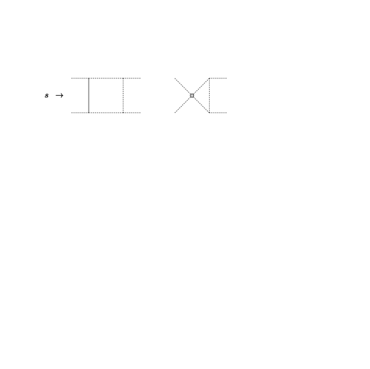
The correspondence is shown in fig.(2) and in fig.(3). In both figures light particles (of mass ) are represented by dashed lines, heavy particles (of mass ) by straight lines. We are interested in the region and . The left diagram (underlying theory) in fig.(2) has a normal threshold at and corresponds to a loop-generated operator (denoted by a black circle) in the corresponding tree-level EFT. The left diagram (underlying theory) in fig.(3) has a normal threshold at and corresponds (one-loop matching) to the right diagram which is one-loop EFT with the insertion of a tree-generated operator (denoted by a grey circle). Therefore, to match amplitudes we also need to compute one-loop scattering amplitude in the effective theory, very much in the same way as indicated in Ref. [113].
The full theory is renormalizable and will yield finite predictions in terms of its renormalized (mixed on-shell and ) parameters [86, 127]. The EFT will have quite different UV properties because it is missing the heavy degrees of freedom (but the divergencies will disappear through the renormalization of Wilson coefficients), however the low energy effects will be similar in both calculations. In particular, the non-local behavior is exactly what is found by taking the low-energy limit of the full theory, expanded to this order [144, 143]. The key advantages are a more precise matching and the appearance of some important kinematic dependence, e.g. also the coefficients of “kinematic” logarithms match [143]; an explicit example, in the linear sigma-model, is shown in sect. of Ref. [143]. As far as normal threshold singularities are concerned we mention that loop calculations should be performed in the so-called complex-mass scheme [145, 146, 147]. As a matter of fact, Ref. [143] underlines that the most important predictions of the EFT are related to non–analytic in momenta loop contributions which modify tails of distributions. For a covariant treatment of logarithms in the EFT expansion Ref. [148] points out that we can use a spectral representation, i.e.
| (219) |
The traditional approach splits the non-local contributions into one-loop EFT diagrams with TG operator insertions (e.g. the “non-loc” term in Eq.(213)), which are not inserted into the EFT Lagrangian and LG operators used at tree level (e.g. first term in Eq.(213)) which constitute the heavy–light contributions to matching. This splitting should be carefully described since triangles, boxes etc have both local and non-local parts, as shown in Eq.(217). The authors of Ref. [143] draw our attention to the fact that non–local effects correspond to long distance propagation and hence to the reliable predictions at low energy. The local terms by contrast summarize the unknown effects from high energy. Having both local and non–local terms allows us to implement the full EFT program.
One way or the other, once the matching is done, all processes can be calculated using the “fitted” (renormalized) Wilson coefficients without the need to match again for each process.
The authors of Ref. [114] use a different language, based on “expansion by regions” [149, 150], separating the hard region contribution from the soft one:
-
hard
-
soft
and reach the conclusion that the EFT Lagrangian at one-loop is then containing only the hard part of the loops.

Low-energy limit, Mellin-Barnes expansion
If we deal with the low-energy limit from a diagrammatic point of view [74] the best technique is given by Mellin-Barnes expansion [151]. Consider a simple example,
| (220) |
where and . We introduce
| (221) |
and derive the following representation in Feynman parameter space,
| (222) |
where must be understood as and as . It follows
| (223) |
which is valid in the vertical strip and where is the Euler beta-function. The integral can be expressed as
| (224) |
giving
| (225) |
Since we are interested in the limit , the -integral will be closed over the left-hand complex half-plane at infinity, with double poles at . Using the well know Laurent and Taylor expansions of the Euler gamma-function we obtain the result summing over the poles; the leading term in the expansion, , gives
| (226) |
showing the large momentum logarithm. For (unphysical region) we can expand the second logarithm in powers of (Taylor expansion); for we are above the normal threshold and the -integral is the UV finite part of a two-point functions, showing the non-local, kinematic, logarithm
| (227) |
To summarize, for , we can Taylor expand only in the region , Note the presence of an imaginary part in Eq.(227), , when . Non-local contributions to the effective Lagrangian usually contain the function
| (228) |
inside a term .
The next term in the expansion is given by the residue of the pole at and gives
| (229) |
showing again large momentum and kinematic logarithms.
9.2 LG operators, results
Heavy scalar, explicit results
Before presenting the list of operators and their coefficients, functions of the parameters in the high-energy theory, some considerations are needed. Following sect. 7 of Ref. [130] we use the fact that, within the BFM algorithm, one may make use of the (BFM) EoMs to simplify the counter-Lagrangian. In our case they read as follows:
| (230) |
where we have taken . From Eq.(190) we find UV poles proportional to
| (231) |
which is zero by virtue of Eq.(230). Staring from Eq.(190) we derive UV divergent terms of , e.g.
| (232) |
which are canceled by a counter-Lagrangian, i.e. we start with
| (233) | |||||
instead ofEq.(159). The remaining terms are as follows:
-
Local
Local operators are shown in tab. 9.2.
We can conceive a scenario where the fit has been performed using the basis [45]
| (234) |
of potentially tree generated operators. The explicit calculation returns the following set of operators:
| (235) |
with equivalence relations
| (236) |
We stress that the equivalence of operators in Eq.(236) is a property of the EFT and can be used to change basis in the EFT while the high-energy theory generates the operators in Eq.(235) with explicit Wilson coefficients given in tab. 9.2. Mapping the parameters of the high-energy theory into the fitted Wilson coefficients corresponding to the operators listed in Eq.(234) requires field transformations at the EFT level with compensations.
| Coefficient | Operator |
|---|---|
-
Non-local
The corresponding contributions can be written as follows:
| non-local | (237) | ||||
where
| (238) |
The functions are combinations of three-point tensor integrals,
| (239) | |||||
where denotes the UV finite part of (for a definition of the -functions see ch. of Ref. [152]). Finally, . It is obvious from Eq.(239) that there is no advantage in deriving the non-local terms with the expansion of Eq.(190); it is actually more convenient to use a diagram-by-diagram calculation in the high-energy theory, followed by an expansion in .
Heavy vectors, explicit results
We have deliberately chosen this example to show the kind of problems that arise when the high-energy theory is not UV complete. This fact should not be confused with a negative statement on renormalizability of the (interacting) Proca theory where one introduces the Stueckelberg ghost [154], into the action of a vector field with a “naive mass term”. In this way the Lagrangian leads to a manifestly gauge invariant action; this gauge invariance remains an exact symmetry, if matter fields are introduced and the vector field is minimally coupled to conserved currents of these fields. This, however, is not the case that we are considering. It is worth mentioning that we are dealing with an accidental property of massive electrodynamics. Massive gauge fields are nonrenormalizable in general, i.e. for a gauge group other than .
In our example the local terms give rise to the following Lagrangian:
| local boson | |||||
| local fermion | (240) | ||||
In conclusion, Wilson coefficients show non renormalizable terms, as expected. This simple example shows the riskiness of extending the SM with new vector bosons having “naive mass terms”; the standard argument against is that longitudinal components do not have a falling off propagator, which means that loops involving longitudinal vectors blow up as a power at high momentum. In gauge theories, gauge invariance guarantees that longitudinal bosons are not produced, but this requires that gauge invariance is broken spontaneously not by the Lagrangian.
10 Interpreting derivative-coupled field theories
An old problem seen through the lens of EFT: consider the following Lagrangian,
| (241) |
where is a Wilson coefficient and is a large scale. We can write with two options
| (242) |
The equation of motion (EoM) gives
| (243) |
The first point to be investigated is the question of separation of the quadratic, i.e. propagator defining, part in . Thus let there be given a Lagrangian
| (244) |
One can either say that one has a propagator for the -field or alternatively a propagator and a vertex . Obviously, the two cases give the same result; however this requires summing over all possible insertions of the vertex , which is different from a truncated expansion in .
10.1 Option a)
Consider in Eq.(242): the first point to be investigated is the validity of Matthews’s theorem [155], i.e. the Feynman rules are just those obtained by using to determine the vertices and the covariant product to determine the propagators (in other words, one can read Feynman rules from the Lagrangian). The validity of the theorem for the Lagrangian of Eq.(241) has been proven long ago in Ref. [156] (see also Ref. [157]) where the authors used an indirect implementation of canonical methods, finding an equivalent Lagrangian which contains only first derivatives but yields the same results (the standard method, originally due to Ostrogradsky [158]). Always in Ref. [156] one can find the spectrum of the theory: there are two masses, solutions of the equation
| (245) |
To exclude tachyons we must have
| (246) |
However, there is a negative metric for the particle with the larger mass, i.e. there is a “ghost” in the spectrum.
In the Ostrogradsky formalism the higher order derivatives are considered to be independent objects; however, this means that new degrees of freedom are introduced. These additional degrees of freedom involve the unphysical effects. To generalize the example consider a operator
| (247) |
Two new fields are needed to write an equivalent first-order Lagrangian
| (248) |
which means that there could be more ghosts in the spectrum; indeed the mass spectrum is given by the values of that satisfy the cubic equation
| (249) |
as it can be seen by inserting the Fourier decomposition for into the corresponding (linear) equation of motion. As a matter of fact all roots are real only if is positive and less tha . However the product of the roots is ; therefore, there is at leat one tachyon in the spectrum.
10.2 Option b)
With option b) one works at first order in . The “dangerous” term (second order derivatives) is substituted by using EoMs where terms of are neglected,
| (250) |
this can be achieved by using the transformation
| (251) |
Of course one could work at second order in , including operators, etc.. The result is
| (252) | |||||
where contains . There is a diagrammatic proof of these relations, see sect. of Ref. [69].
To summarize
EoMs can be applied in order to covert terms in the interaction Lagrangian [67]; the statement is nontrivial because, in general, EoMs must not be inserted into the Lagrangian. However, one can find field transformations which have the same effect as the application of EoMs and yield Lagrangians that are physically equivalent, see Refs. [79, 67, 68]. A field redefinition [5, 68] absorbs the first two terms in Eq.(13) in the part of the Lagrangian while the rest is treated as an interaction term. This is the strategy adopted in Ref. [17] to construct the Standard Model effective field theory (SMEFT).
Therefore, option b) is an effective realization of the original Lagrangian, where one assumes that the effective theory will be replaced by a “well-behaved” new theory at some larger scale, therefore justifying a truncated perturbative expansion in , even in the quadratic part of the Lagrangian. To summarize, option b) is based on the supposed existence of a “well-behaved” UV completion which justifies the omission of all unphysical effects. It is worth noting, see Ref. [157], that the assumption alone is not sufficient since theories with higher derivatives have no analytic limit for . For more details on higher derivative Lagrangians see Refs. [159, 160, 161].
Nevertheless, option a) (10.1) tells us something about the range of validity of the effective Lagrangian, i.e.
-
1.
(no tachyons),
-
2.
, where is the upper real (positive) root of Eq.(245) and is the scale at which we test the predictions of the effective Lagrangian, i.e. must be well below the region where the (resummed) theory develops ghosts.
In the realistic SMEFT scenario, bases for effective field theories [45], the so-called Warsaw basis [17] in particular, are constructed by using the fact that all possible operators in class (where now is a covariant derivative) reduce by EoMs either to operators containing fermions or to classes and , where is any of the SM field strength tensors. Keeping instead the class in the zeroth order Hamiltonian would be equivalent to option a).
Theories obtained by canonical quantization of a second-order Lagrangian, option a), are completely equivalent to the Pauli-Villars regularization of the corresponding first-order theories. However, the regulator mass is not here taken to infinity [156]. Other examples can be found in Refs. [162, 163], Abelian gauge theory with a term; in Ref. [164], with a whole extension of the Standard Model inserting quadratic differential operators; Ref. [165] discusses effective field theory for general scalar-tensor theories;
Finally, let us consider a top-down approach: in any complete theory a term is part of the (light) two-point function with heavy-heavy or light-heavy internal lines. In this case we compute the light-light self-energy and then Dyson resum the light propagator. At this point we expand in the heavy scale, perform mass renormalization for the light particle and get corrections to the light particle wave function. One could think of moving these terms from the EFT interaction Lagrangian to the wave-function of the light degree of freedom; however, resumming a class of higher order EFT effects implies that EFT has not been consistently used in the matching 777I am grateful to M. Trott for this comment..
11 Conclusions
In this work 888Some of the issues discussed in this paper partially overlap with the very recent work of Ref. [166]. we have examined the relationship among a four-dimensional, weakly coupled, field theory , its EFT extension and the class of UV completions of , say . Technically speaking we are interested in constructing up to and including operators.
In developing the SM EFT there is a dual motivation for including operators: it may prove that an analysis purely at the level is inadequate, or that effects should be accounted for as a systematic uncertainty. Indeed, given the plethora of new physics scenarios that may show up in future precision Higgs measurements only at the percent level, it is an urgent issue to understand and reduce theory uncertainties so that they do not become a limiting factor in our searches for new physics.
As stated in the Introduction, EFT is being widely used in an effort to interpret experimental measurements of SM processes. In this scenario, various consistency issues arise; we have critically examined the issues and argued for the necessity to learn more general lessons about new physics within the EFT approach.
Every EFT extension of is a consistent QFT, although differing from in the UV, i.e. we can calculate in the EFT without unnecessary reference to the UV physics that is is decoupled. However, if the value of Wilson coefficients in broad UV scenarios could be inferred in general this would be of significant scientific value. Therefore, the central question in top-down EFT studies is: given a UV theory, what is the low-energy EFT, and what are its observable consequences? The answer to this question is of course UV theory specific. We have discussed this scenario from the point of view of the higher order compensations arising from the removal of “redundant” operators.
The classical LSZ formalism [167] is better handled by using the so-called “canonical normalization”; we have discussed the interply between canonical normalization, gauge invariance and gauge fixing. Actually, canonical normalization should be understood in a broad sense: corrections to operators are reabsorbed into the parameters of the Lagrangian. From this point of view it is more convenient to work with the -gauge [146], so that the gauge parameters can also be normalized. Canonical normalization for the tadpole parameter, which is not strictly needed for SMEFT at LO, will play an important role when constructing SMEFT at NLO [60, 5].
When considering the SM the EFTs are further distinguished by the presence of a Higgs doublet (or not) in the construction. In the SMEFT the EFT is constructed with an explicit Higgs doublet, while in the HEFT (an Electroweak chiral Lagrangian with a dominantly scalar) no such doublet is included. Usability of SMEFT/HEFT in UV scenarios based on a proliferation of scalars and mixings has also been discussed.
We have analyzed the impact on global fits of different effects: selection of a basis, transformation of basis, truncation of basis, inclusion/exclusion of canonical normalization. All of them go in the same direction: inconsistent results usually attributed to SMEFT are in fact the consequence of unnecessary further approximations and multiple operators, after canonical normalization, should be retained in data analyses. Effective field theories accomplish internal consistency; quite often, when EFTs are considered in the actual practice, only a limited set of terms is used destroying the mathematical consistency. Precision tests of the SM in all sectors and critical examination of the EFT framework have become more important than ever.
A key ingredient of top-down EFT studies is matching a given UV theory onto its low-energy EFT. By this we mean that, after the Higgs boson discovery, we have a paradigm shift, i.e. we use the EFT for fitting the data. The “fitted” Wilson coefficients become the pseudo-data and we may take any specific BSM model, compute the corresponding low-energy limit and choose the BSM parameters to be those appropriate for the pseudo-data.
There are elegant methods for obtaining operator coefficients, which avoid the need for computing complicated correlation functions. They are based on direct evaluation of the functional path integral and we have analyzed in details some of the subtle points which arise during the process, proper handling of matrix logarithms and non-local terms due to heavy-light contributions. We argue for the key advantages of having a more precise, one-loop, matching. An insurgence of non-local terms in the effective action is due to heavy-light effects, although not all of them have a non-local character (of the form of kinematic logarithms), which is controlled by loop diagrams having normal, as well as anomalous, thresholds in the low-energy region.
Finally, we have reviewed the effective field theory interpretation of derivative-coupled field theories.
The BSM picture is still incomplete. Paraphrasing Freeman Dyson [168], we can say that some physicists are birds, others are frogs. Birds fly high in the air (top-down approach) and survey broad vistas out to the far horizon. Frogs live in the mud below (bottom-up approach) and see only the flowers that grow nearby. They solve problems one at a time. BSM physics needs both birds and frogs. Physics is rich and beautiful because birds give it broad visions and frogs give it intricate details (this paper happens to be a frog).
Acknowledgments: I gratefully acknowledge a constructive correspondence with A. David.
Appendix A Field transformations and their Jacobian
Consider a theory with one scalar field and a transformation . As it is well known this transformation has several effects, including the presence of a Jacobian in the functional integral. The latter shows up as a ghost Lagrangian (not the FP ghosts however)
| (253) |
The reason why this part of the Lagrangian does note contribute is explained in sect. of Ref. [41]. Here we want to repeat the argument by giving the proper emphasis to a crucial aspect of any EFT, local-analytic expansion in EFT as described in Ref. [4]. The ghost propagator is
| (254) |
Suppose that we want to use this propagator inside EFT loop diagrams, e.g. for the -point function. It is immediately seen that loop integration and limit are non-commuting operations. In particular,
| (255) |
which means that -loops are zero in dimensional regularization when the limit is first. That one has to expand first is inherent to EFT, as explained in sect. of Ref. [4] and it is due to “separation of scales” and to the fact that the result of integrating havy degrees of freedom is an effective action that describes non-local interactions between the low-energy degrees of freedom. To obtain a local effective action the effective action is expanded in terms of local operators [169].
Appendix B Higher dimensional operators and FP ghosts
If is the SM and SMEFT is constructed according to Eq.(1), what about FP ghost fields in ? This question is only relevant for NLO SMEFT, nevertheless let us examine the situation in more details. Suppose that is the singlet extension of the SM; after fixing the gauge in and taking the mixing into account we will have couplings between the heavy Higgs, , and FP-fields, e.g. . At the same time there are couplings so that we can generate (in ) a tree-level diagram with external lines and one internal line. After expanding the propagator we obtain an effective vertex with only light fields and FP fields; this vertex can be used to construct EFT loops contributing to . This fact raises the question of whether -dimensional operators containing FP ghosts should be included in the EFT Lagrangian.
Appendix C Tadpole and log-tadpole integrals
Tadpole integrals are defined as follows:
| (256) |
which vanishes for odd values of and gives
| (257) |
We need to evaluate
| (258) |
with and . We derive
| (263) | |||||
where we have defined
| (264) |
From Eq.(263) we see that the functions always appear in the combination
| (265) |
with , id the Euler-Mascheroni constant and is the ’t Hooft scale.
- Log-tadpoles
In deriving the result we have used [170]
| (266) |
etc. More log-tadpole integrals are need;
| (267) |
is defined in the strip . The explicit result is
| (268) |
We also need with . The integral is defined for etc. By analytic continuation we obtain
| (269) |
while shows a double pole.
References
- [1] K. Yagyu, Studies on Extended Higgs Sectors as a Probe of New Physics Beyond the Standard Model, Ph.D. thesis, Toyama U. (2012). arXiv:1204.0424.
- [2] G. Altarelli, D. Meloni, A non supersymmetric SO(10) grand unified model for all the physics below , JHEP 08 (2013) 021. arXiv:1305.1001, doi:10.1007/JHEP08(2013)021.
- [3] H. Okada, N. Okada, Y. Orikasa, K. Yagyu, Higgs phenomenology in the minimal SU(3)L×U(1)X model, Phys. Rev. D94 (1) (2016) 015002. arXiv:1604.01948, doi:10.1103/PhysRevD.94.015002.
- [4] I. Brivio, M. Trott, The Standard Model as an Effective Field TheoryarXiv:1706.08945.
- [5] G. Passarino, M. Trott, The Standard Model Effective Field Theory and Next to Leading OrderarXiv:1610.08356.
- [6] J. Bain, Effective field theories, in: R. Batterman (Ed.), The Oxford Handbook of Philosophy of Physics, Oup Usa, 2013, p. 224.
- [7] A. Freitas, D. López-Val, T. Plehn, When matching matters: Loop effects in Higgs effective theory, Phys. Rev. D94 (9) (2016) 095007. arXiv:1607.08251, doi:10.1103/PhysRevD.94.095007.
- [8] A. Biekötter, J. Brehmer, T. Plehn, Extending the limits of Higgs effective theory, Phys. Rev. D94 (5) (2016) 055032. arXiv:1602.05202, doi:10.1103/PhysRevD.94.055032.
- [9] M. Boggia, R. Gomez-Ambrosio, G. Passarino, Low energy behaviour of standard model extensions, JHEP 05 (2016) 162. arXiv:1603.03660, doi:10.1007/JHEP05(2016)162.
- [10] M. J. G. Veltman, Generalized Ward identities and Yang-Mills fields, Nucl. Phys. B 21 (1970) 288–302. doi:10.1016/0550-3213(70)90478-5.
- [11] J. Taylor, Ward Identities and Charge Renormalization of the Yang-Mills Field, Nucl. Phys. B 33 (1971) 436–444. doi:10.1016/0550-3213(71)90297-5.
- [12] A. Slavnov, Ward Identities in Gauge Theories, Theor. Math. Phys. 10 (1972) 99–107. doi:10.1007/BF01090719,10.1007/BF01090719.
- [13] M. S. Bilenky, A. Santamaria, One loop effective Lagrangian for a standard model with a heavy charged scalar singlet, Nucl. Phys. B420 (1994) 47–93. arXiv:hep-ph/9310302, doi:10.1016/0550-3213(94)90375-1.
- [14] C.-W. Chiang, R. Huo, Standard Model Effective Field Theory: Integrating out a Generic Scalar, JHEP 09 (2015) 152. arXiv:1505.06334, doi:10.1007/JHEP09(2015)152.
- [15] M. Gorbahn, J. M. No, V. Sanz, Benchmarks for Higgs Effective Theory: Extended Higgs Sectors, JHEP 10 (2015) 036. arXiv:1502.07352, doi:10.1007/JHEP10(2015)036.
- [16] S. Dawson, C. W. Murphy, Standard Model EFT and Extended Scalar Sectors, Phys. Rev. D96 (1) (2017) 015041. arXiv:1704.07851, doi:10.1103/PhysRevD.96.015041.
- [17] B. Grzadkowski, M. Iskrzynski, M. Misiak, J. Rosiek, Dimension-Six Terms in the Standard Model Lagrangian, JHEP 10 (2010) 085. arXiv:1008.4884, doi:10.1007/JHEP10(2010)085.
- [18] M. B. Gavela, K. Kanshin, P. A. N. Machado, S. Saa, On the renormalization of the electroweak chiral Lagrangian with a Higgs, JHEP 03 (2015) 043. arXiv:1409.1571, doi:10.1007/JHEP03(2015)043.
- [19] I. Brivio, T. Corbett, O. J. P. Éboli, M. B. Gavela, J. Gonzalez-Fraile, M. C. Gonzalez-Garcia, L. Merlo, S. Rigolin, Disentangling a dynamical Higgs, JHEP 03 (2014) 024. arXiv:1311.1823, doi:10.1007/JHEP03(2014)024.
- [20] R. Alonso, E. E. Jenkins, A. V. Manohar, A Geometric Formulation of Higgs Effective Field Theory: Measuring the Curvature of Scalar Field Space, Phys. Lett. B754 (2016) 335–342. arXiv:1511.00724, doi:10.1016/j.physletb.2016.01.041.
- [21] G. Buchalla, O. Cata, A. Celis, C. Krause, Fitting Higgs Data with Nonlinear Effective Theory, Eur. Phys. J. C76 (5) (2016) 233. arXiv:1511.00988, doi:10.1140/epjc/s10052-016-4086-9.
- [22] J. J. Sanz-Cillero, Resonances and loops: scale interplay in the Higgs effective field theory, PoS EPS-HEP2017 (2017) 460. arXiv:1710.07611, doi:10.22323/1.314.0460.
- [23] S. Dawson, I. M. Lewis, Singlet Model Interference Effects with High Scale UV Physics, Phys. Rev. D95 (1) (2017) 015004. arXiv:1605.04944, doi:10.1103/PhysRevD.95.015004.
- [24] F. del Aguila, J. de Blas, M. Perez-Victoria, Electroweak Limits on General New Vector Bosons, JHEP 09 (2010) 033. arXiv:1005.3998, doi:10.1007/JHEP09(2010)033.
- [25] F. del Aguila, M. Perez-Victoria, J. Santiago, Observable contributions of new exotic quarks to quark mixing, JHEP 09 (2000) 011. arXiv:hep-ph/0007316, doi:10.1088/1126-6708/2000/09/011.
- [26] F. del Aguila, J. de Blas, M. Perez-Victoria, Effects of new leptons in Electroweak Precision Data, Phys. Rev. D78 (2008) 013010. arXiv:0803.4008, doi:10.1103/PhysRevD.78.013010.
- [27] J. de Blas, M. Chala, M. Perez-Victoria, J. Santiago, Observable Effects of General New Scalar Particles, JHEP 04 (2015) 078. arXiv:1412.8480, doi:10.1007/JHEP04(2015)078.
- [28] J. de Blas, J. C. Criado, M. Perez-Victoria, J. Santiago, Effective description of general extensions of the Standard Model: the complete tree-level dictionary, JHEP 03 (2018) 109. arXiv:1711.10391, doi:10.1007/JHEP03(2018)109.
- [29] H. E. Haber, Approximate Higgs alignment without decoupling, in: 53rd Rencontres de Moriond on QCD and High Energy Interactions (Moriond QCD 2018) La Thuile, Italy, March 17-24, 2018, 2018. arXiv:1805.05754.
- [30] B. Grzadkowski, H. E. Haber, O. M. Ogreid, P. Osland, Heavy Higgs boson decays in the alignment limit of the 2HDMarXiv:1808.01472.
- [31] R. Barbieri, L. J. Hall, V. S. Rychkov, Improved naturalness with a heavy Higgs: An Alternative road to LHC physics, Phys. Rev. D74 (2006) 015007. arXiv:hep-ph/0603188, doi:10.1103/PhysRevD.74.015007.
- [32] E. E. Jenkins, A. V. Manohar, P. Stoffer, Low-Energy Effective Field Theory below the Electroweak Scale: Operators and Matching, JHEP 03 (2018) 016. arXiv:1709.04486, doi:10.1007/JHEP03(2018)016.
- [33] E. E. Jenkins, A. V. Manohar, P. Stoffer, Low-Energy Effective Field Theory below the Electroweak Scale: Anomalous Dimensions, JHEP 01 (2018) 084. arXiv:1711.05270, doi:10.1007/JHEP01(2018)084.
- [34] J. D. Wells, Z. Zhang, Y. Zhao, Establishing the Isolated Standard Model, Phys. Rev. D96 (1) (2017) 015005. arXiv:1702.06954, doi:10.1103/PhysRevD.96.015005.
- [35] J. D. Wells, Higgs naturalness and the scalar boson proliferation instability problem, Synthese 194 (2) (2017) 477–490. arXiv:1603.06131, doi:10.1007/s11229-014-0618-8.
- [36] A. Barzinji, M. Trott, A. Vasudevan, Equations of Motion for the Standard Model Effective Field Theory: Theory and ApplicationsarXiv:1806.06354.
- [37] A. Helset, M. Trott, Equations of motion, symmetry currents and EFT below the electroweak scalearXiv:1812.02991.
- [38] W. Buchmuller, D. Wyler, Effective Lagrangian Analysis of New Interactions and Flavor Conservation, Nucl.Phys. B268 (1986) 621. doi:10.1016/0550-3213(86)90262-2.
- [39] H. Simma, Equations of motion for effective Lagrangians and penguins in rare B decays, Z. Phys. C61 (1994) 67–82. arXiv:hep-ph/9307274, doi:10.1007/BF01641888.
- [40] H. D. Politzer, Power Corrections at Short Distances, Nucl. Phys. B172 (1980) 349–382. doi:10.1016/0550-3213(80)90172-8.
- [41] C. Arzt, M. B. Einhorn, J. Wudka, Patterns of deviation from the standard model, Nucl. Phys. B433 (1995) 41–66. arXiv:hep-ph/9405214, doi:10.1016/0550-3213(94)00336-D.
- [42] C. P. Burgess, Introduction to Effective Field Theory, Ann. Rev. Nucl. Part. Sci. 57 (2007) 329–362. arXiv:hep-th/0701053, doi:10.1146/annurev.nucl.56.080805.140508.
- [43] W. D. Goldberger, Les Houches lectures on effective field theories and gravitational radiation, in: Les Houches Summer School - Session 86: Particle Physics and Cosmology: The Fabric of Spacetime Les Houches, France, July 31-August 25, 2006, 2007. arXiv:hep-ph/0701129.
- [44] W. Skiba, Effective Field Theory and Precision Electroweak Measurements, in: Physics of the large and the small, TASI 09, proceedings of the Theoretical Advanced Study Institute in Elementary Particle Physics, Boulder, Colorado, USA, 1-26 June 2009, 2011, pp. 5–70. arXiv:1006.2142, doi:10.1142/9789814327183_0001.
- [45] M. B. Einhorn, J. Wudka, The Bases of Effective Field Theories, Nucl. Phys. B876 (2013) 556–574. arXiv:1307.0478, doi:10.1016/j.nuclphysb.2013.08.023.
- [46] A. Dedes, W. Materkowska, M. Paraskevas, J. Rosiek, K. Suxho, Feynman rules for the Standard Model Effective Field Theory in -gauges, JHEP 06 (2017) 143. arXiv:1704.03888, doi:10.1007/JHEP06(2017)143.
- [47] S. Das Bakshi, J. Chakrabortty, S. K. Patra, CoDEx: Wilson coefficient calculator connecting SMEFT to UV theoryarXiv:1808.04403.
- [48] B. Gripaios, D. Sutherland, DEFT: A program for operators in EFTarXiv:1807.07546.
- [49] J. C. Criado, BasisGen: automatic generation of operator basesarXiv:1901.03501.
- [50] L. Lehman, A. Martin, Hilbert Series for Constructing Lagrangians: expanding the phenomenologist’s toolbox, Phys. Rev. D91 (2015) 105014. arXiv:1503.07537, doi:10.1103/PhysRevD.91.105014.
- [51] L. Lehman, A. Martin, Low-derivative operators of the Standard Model effective field theory via Hilbert series methods, JHEP 02 (2016) 081. arXiv:1510.00372, doi:10.1007/JHEP02(2016)081.
- [52] B. Henning, X. Lu, T. Melia, H. Murayama, Hilbert series and operator bases with derivatives in effective field theories, Commun. Math. Phys. 347 (2) (2016) 363–388. arXiv:1507.07240, doi:10.1007/s00220-015-2518-2.
- [53] B. Henning, X. Lu, T. Melia, H. Murayama, 2, 84, 30, 993, 560, 15456, 11962, 261485, …: Higher dimension operators in the SM EFT, JHEP 08 (2017) 016. arXiv:1512.03433, doi:10.1007/JHEP08(2017)016.
- [54] B. Henning, X. Lu, T. Melia, H. Murayama, Operator bases, -matrices, and their partition functions, JHEP 10 (2017) 199. arXiv:1706.08520, doi:10.1007/JHEP10(2017)199.
- [55] J. Wudka, Electroweak effective Lagrangians, Int. J. Mod. Phys. A9 (1994) 2301–2362. arXiv:hep-ph/9406205, doi:10.1142/S0217751X94000959.
- [56] E. E. Jenkins, A. V. Manohar, M. Trott, On Gauge Invariance and Minimal Coupling, JHEP 09 (2013) 063. arXiv:1305.0017, doi:10.1007/JHEP09(2013)063.
- [57] B. Gripaios, Lectures on Effective Field TheoryarXiv:1506.05039.
- [58] R. Alonso, E. E. Jenkins, A. V. Manohar, Holomorphy without Supersymmetry in the Standard Model Effective Field Theory, Phys. Lett. B739 (2014) 95–98. arXiv:1409.0868, doi:10.1016/j.physletb.2014.10.045.
- [59] C. Cheung, C.-H. Shen, Nonrenormalization Theorems without Supersymmetry, Phys. Rev. Lett. 115 (7) (2015) 071601. arXiv:1505.01844, doi:10.1103/PhysRevLett.115.071601.
- [60] M. Ghezzi, R. Gomez-Ambrosio, G. Passarino, S. Uccirati, NLO Higgs effective field theory and kappa-framework, JHEP 07 (2015) 175. arXiv:1505.03706, doi:10.1007/JHEP07(2015)175.
- [61] G. Passarino, SMEFT, a theory for SM deviations, PoS ICHEP2016 (2016) 400.
- [62] A. V. Manohar, M. B. Wise, Modifications to the properties of the Higgs boson, Phys. Lett. B636 (2006) 107–113. arXiv:hep-ph/0601212, doi:10.1016/j.physletb.2006.03.030.
- [63] A. V. Manohar, M. B. Wise, Flavor changing neutral currents, an extended scalar sector, and the Higgs production rate at the CERN LHC, Phys. Rev. D74 (2006) 035009. arXiv:hep-ph/0606172, doi:10.1103/PhysRevD.74.035009.
- [64] A. V. Manohar, An Exactly Solvable Model for Dimension Six Higgs Operators and , Phys. Lett. B726 (2013) 347–351. arXiv:1305.3927, doi:10.1016/j.physletb.2013.08.072.
- [65] B. Henning, X. Lu, H. Murayama, How to use the Standard Model effective field theory, JHEP 01 (2016) 023. arXiv:1412.1837, doi:10.1007/JHEP01(2016)023.
- [66] S. Scherer, H. W. Fearing, Field transformations and the classical equation of motion in chiral perturbation theory, Phys. Rev. D52 (1995) 6445–6450. arXiv:hep-ph/9408298, doi:10.1103/PhysRevD.52.6445.
- [67] C. Arzt, Reduced effective Lagrangians, Phys. Lett. B342 (1995) 189–195. arXiv:hep-ph/9304230, doi:10.1016/0370-2693(94)01419-D.
- [68] G. Passarino, Field reparametrization in effective field theories, Eur. Phys. J. Plus 132 (1) (2017) 16. arXiv:1610.09618, doi:10.1140/epjp/i2017-11291-5.
-
[69]
G. ’t Hooft, M. J. G. Veltman,
Diagrammar, CERN Yellow Reports:
Monographs, CERN, Geneva, 1973.
URL http://cds.cern.ch/record/186259 - [70] C. Hays, A. Martin, V. Sanz, J. Setford, On the impact of dimension-eight SMEFT operators on Higgs measurementsarXiv:1808.00442.
- [71] A. V. Manohar, The HQET / NRQCD Lagrangian to order , Phys. Rev. D56 (1997) 230–237. arXiv:hep-ph/9701294, doi:10.1103/PhysRevD.56.230.
- [72] M. Jiang, N. Craig, Y.-Y. Li, D. Sutherland, Complete One-Loop Matching for a Singlet Scalar in the Standard Model EFTarXiv:1811.08878.
- [73] B. Grinstein, M. B. Wise, Operator analysis for precision electroweak physics, Phys. Lett. B265 (1991) 326–334. doi:10.1016/0370-2693(91)90061-T.
- [74] G. Passarino, NLO Inspired Effective Lagrangians for Higgs Physics, Nucl. Phys. B868 (2013) 416–458. arXiv:1209.5538, doi:10.1016/j.nuclphysb.2012.11.018.
- [75] J. R. Andersen, et al., Handbook of LHC Higgs Cross Sections: 3. Higgs PropertiesarXiv:1307.1347, doi:10.5170/CERN-2013-004.
- [76] M. B. Einhorn, J. Wudka, Effective beta functions for effective field theory, JHEP 08 (2001) 025. arXiv:hep-ph/0105035, doi:10.1088/1126-6708/2001/08/025.
- [77] A. Helset, M. Paraskevas, M. Trott, Gauge fixing the Standard Model Effective Field Theory, Phys. Rev. Lett. 120 (25) (2018) 251801. arXiv:1803.08001, doi:10.1103/PhysRevLett.120.251801.
- [78] K. Costello, Renormalization and Effective Field Theory, Mathematical Surveys and Monographs Volume , American Mathematical Society (2011).
- [79] R. E. Kallosh, I. V. Tyutin, The Equivalence theorem and gauge invariance in renormalizable theories, Yad. Fiz. 17 (1973) 190–209, [Sov. J. Nucl. Phys.17,98(1973)].
- [80] M. Misiak, M. Paraskevas, J. Rosiek, K. Suxho, B. Zglinicki, Effective Field Theories in gaugesarXiv:1812.11513.
- [81] G. ’t Hooft, M. J. G. Veltman, Combinatorics of gauge fields, Nucl. Phys. B50 (1972) 318–353. doi:10.1016/S0550-3213(72)80021-X.
- [82] C. Becchi, A. Rouet, R. Stora, Renormalization of the Abelian Higgs-Kibble Model, Commun. Math. Phys. 42 (1975) 127–162. doi:10.1007/BF01614158.
- [83] C. Becchi, A. Rouet, R. Stora, Renormalization of Gauge Theories, Annals Phys. 98 (1976) 287–321. doi:10.1016/0003-4916(76)90156-1.
- [84] S. Actis, A. Ferroglia, M. Passera, G. Passarino, Two-Loop Renormalization in the Standard Model. Part I: Prolegomena, Nucl. Phys. B777 (2007) 1–34. arXiv:hep-ph/0612122, doi:10.1016/j.nuclphysb.2007.04.021.
- [85] J. Fleischer, F. Jegerlehner, Radiative Corrections to Higgs Decays in the Extended Weinberg-Salam Model, Phys. Rev. D23 (1981) 2001–2026. doi:10.1103/PhysRevD.23.2001.
- [86] A. Denner, L. Jenniches, J.-N. Lang, C. Sturm, Gauge-independent renormalization in the 2HDM, JHEP 09 (2016) 115. arXiv:1607.07352, doi:10.1007/JHEP09(2016)115.
- [87] C. Degrande, A basis of dimension-eight operators for anomalous neutral triple gauge boson interactions, JHEP 02 (2014) 101. arXiv:1308.6323, doi:10.1007/JHEP02(2014)101.
- [88] A. Senol, H. Denizli, A. Yilmaz, I. Turk Cakir, K. Y. Oyulmaz, O. Karadeniz, O. Cakir, Probing the Effects of Dimension-eight Operators Describing Anomalous Neutral Triple Gauge Boson Interactions at FCC-hh, Nucl. Phys. B935 (2018) 365–376. arXiv:1805.03475, doi:10.1016/j.nuclphysb.2018.08.018.
- [89] M. K. Gaillard, The Effective One Loop Lagrangian With Derivative Couplings, Nucl. Phys. B268 (1986) 669–692. doi:10.1016/0550-3213(86)90264-6.
- [90] O. Cheyette, Effective Action for the Standard Model With Large Higgs Mass, Nucl. Phys. B297 (1988) 183–204. doi:10.1016/0550-3213(88)90205-2.
- [91] S. Dittmaier, C. Grosse-Knetter, Deriving nondecoupling effects of heavy fields from the path integral: A Heavy Higgs field in an SU(2) gauge theory, Phys. Rev. D52 (1995) 7276–7293. arXiv:hep-ph/9501285, doi:10.1103/PhysRevD.52.7276.
- [92] S. Dittmaier, C. Grosse-Knetter, Integrating out the standard Higgs field in the path integral, Nucl. Phys. B459 (1996) 497–536. arXiv:hep-ph/9505266, doi:10.1016/0550-3213(95)00551-X.
- [93] L. Reina, J. de Blas, M. Ciuchini, E. Franco, D. Ghosh, S. Mishima, M. Pierini, L. Silvestrini, Precision constraints on non-standard Higgs-boson couplings with HEPfit, PoS EPS-HEP2015 (2015) 187. doi:10.22323/1.234.0187.
- [94] M. Bjørn, M. Trott, Interpreting mass measurements in the SMEFT, Phys. Lett. B762 (2016) 426–431. arXiv:1606.06502, doi:10.1016/j.physletb.2016.10.003.
- [95] L. Berthier, M. Bjørn, M. Trott, Incorporating doubly resonant data in a global fit of SMEFT parameters to lift flat directions, JHEP 09 (2016) 157. arXiv:1606.06693, doi:10.1007/JHEP09(2016)157.
- [96] A. Buckley, C. Englert, J. Ferrando, D. J. Miller, L. Moore, K. Nördstrom, M. Russell, C. D. White, Results from TopFitter, PoS CKM2016 (2016) 127. arXiv:1612.02294, doi:10.22323/1.291.0127.
- [97] C. Mariotti, G. Passarino, Higgs boson couplings: measurements and theoretical interpretation, Int. J. Mod. Phys. A32 (04) (2017) 1730003. arXiv:1612.00269, doi:10.1142/S0217751X17300034.
- [98] I. Brivio, Y. Jiang, M. Trott, The SMEFTsim package, theory and tools, JHEP 12 (2017) 070. arXiv:1709.06492, doi:10.1007/JHEP12(2017)070.
- [99] C. W. Murphy, Statistical approach to Higgs boson couplings in the standard model effective field theory, Phys. Rev. D97 (1) (2018) 015007. arXiv:1710.02008, doi:10.1103/PhysRevD.97.015007.
- [100] S. Alte, M. König, W. Shepherd, Consistent Searches for SMEFT Effects in Non-Resonant Dijet Events, JHEP 01 (2018) 094. arXiv:1711.07484, doi:10.1007/JHEP01(2018)094.
- [101] J. Ellis, C. W. Murphy, V. Sanz, T. You, Updated Global SMEFT Fit to Higgs, Diboson and Electroweak Data, JHEP 06 (2018) 146. arXiv:1803.03252, doi:10.1007/JHEP06(2018)146.
- [102] J. Aebischer, J. Kumar, P. Stangl, D. M. Straub, A Global Likelihood for Precision Constraints and Flavour AnomaliesarXiv:1810.07698.
- [103] D. Barducci, et al., Interpreting top-quark LHC measurements in the standard-model effective field theoryarXiv:1802.07237.
- [104] S. Wesolowski, N. Klco, R. J. Furnstahl, D. R. Phillips, A. Thapaliya, Bayesian parameter estimation for effective field theories, J. Phys. G43 (7) (2016) 074001. arXiv:1511.03618, doi:10.1088/0954-3899/43/7/074001.
- [105] S. Kanemura, M. Kikuchi, K. Mawatari, K. Sakurai, K. Yagyu, Loop effects on the Higgs decay widths in extended Higgs models, Phys. Lett. B783 (2018) 140–149. arXiv:1803.01456, doi:10.1016/j.physletb.2018.06.035.
- [106] M. J. G. Veltman, Limit on Mass Differences in the Weinberg Model, Nucl. Phys. B123 (1977) 89–99. doi:10.1016/0550-3213(77)90342-X.
- [107] M. B. Einhorn, D. R. T. Jones, M. J. G. Veltman, Heavy Particles and the rho Parameter in the Standard Model, Nucl. Phys. B191 (1981) 146–172. doi:10.1016/0550-3213(81)90292-3.
- [108] I. Low, J. Lykken, G. Shaughnessy, Have We Observed the Higgs (Imposter)?, Phys. Rev. D86 (2012) 093012. arXiv:1207.1093, doi:10.1103/PhysRevD.86.093012.
- [109] I. Brivio, J. Gonzalez-Fraile, M. C. Gonzalez-Garcia, L. Merlo, The complete HEFT Lagrangian after the LHC Run I, Eur. Phys. J. C76 (7) (2016) 416. arXiv:1604.06801, doi:10.1140/epjc/s10052-016-4211-9.
- [110] B. M. Gavela, E. E. Jenkins, A. V. Manohar, L. Merlo, Analysis of General Power Counting Rules in Effective Field Theory, Eur. Phys. J. C76 (9) (2016) 485. arXiv:1601.07551, doi:10.1140/epjc/s10052-016-4332-1.
- [111] F. del Aguila, Z. Kunszt, J. Santiago, One-loop effective lagrangians after matching, Eur. Phys. J. C76 (5) (2016) 244. arXiv:1602.00126, doi:10.1140/epjc/s10052-016-4081-1.
- [112] B. Henning, X. Lu, H. Murayama, One-loop Matching and Running with Covariant Derivative Expansion, JHEP 01 (2018) 123. arXiv:1604.01019, doi:10.1007/JHEP01(2018)123.
- [113] S. A. R. Ellis, J. Quevillon, T. You, Z. Zhang, Mixed heavy–light matching in the Universal One-Loop Effective Action, Phys. Lett. B762 (2016) 166–176. arXiv:1604.02445, doi:10.1016/j.physletb.2016.09.016.
- [114] J. Fuentes-Martin, J. Portoles, P. Ruiz-Femenia, Integrating out heavy particles with functional methods: a simplified framework, JHEP 09 (2016) 156. arXiv:1607.02142, doi:10.1007/JHEP09(2016)156.
- [115] J. Braathen, M. D. Goodsell, P. Slavich, Matching renormalisable couplings: simple schemes and a plotarXiv:1810.09388.
- [116] Q. Mou, S. Zheng, A Heavy Scalar at the LHC from Vector Boson Fusion, Adv. High Energy Phys. 2018 (2018) 9314613. arXiv:1508.06014, doi:10.1155/2018/9314613.
- [117] R. Alonso, E. E. Jenkins, A. V. Manohar, Geometry of the Scalar Sector, JHEP 08 (2016) 101. arXiv:1605.03602, doi:10.1007/JHEP08(2016)101.
- [118] S. Willenbrock, C. Zhang, Effective Field Theory Beyond the Standard Model, Ann. Rev. Nucl. Part. Sci. 64 (2014) 83–100. arXiv:1401.0470, doi:10.1146/annurev-nucl-102313-025623.
- [119] Y. Jiang, M. Trott, On the non-minimal character of the SMEFT, Phys. Lett. B770 (2017) 108–116. arXiv:1612.02040, doi:10.1016/j.physletb.2017.04.053.
- [120] J. Brehmer, A. Freitas, D. Lopez-Val, T. Plehn, Pushing Higgs Effective Theory to its Limits, Phys. Rev. D93 (7) (2016) 075014. arXiv:1510.03443, doi:10.1103/PhysRevD.93.075014.
- [121] M. Boggia, et al., The HiggsTools Handbook: Concepts and observables for deciphering the Nature of the Higgs SectorarXiv:1711.09875.
- [122] C. Degrande, B. Fuks, K. Mawatari, K. Mimasu, V. Sanz, Electroweak Higgs boson production in the standard model effective field theory beyond leading order in QCD, Eur. Phys. J. C77 (4) (2017) 262. arXiv:1609.04833, doi:10.1140/epjc/s10052-017-4793-x.
- [123] R. Gomez-Ambrosio, Studies of Dimension-Six EFT effects in Vector Boson ScatteringarXiv:1809.04189.
- [124] J. Brehmer, K. Cranmer, F. Kling, T. Plehn, Better Higgs boson measurements through information geometry, Phys. Rev. D95 (7) (2017) 073002. arXiv:1612.05261, doi:10.1103/PhysRevD.95.073002.
- [125] J. Brehmer, K. Cranmer, G. Louppe, J. Pavez, A Guide to Constraining Effective Field Theories with Machine Learning, Phys. Rev. D98 (5) (2018) 052004. arXiv:1805.00020, doi:10.1103/PhysRevD.98.052004.
- [126] D. Yu. Bardin, M. Grunewald, G. Passarino, Precision calculation project reportarXiv:hep-ph/9902452.
- [127] L. Altenkamp, S. Dittmaier, H. Rzehak, Precision calculations for fermions in the Two-Higgs-Doublet Model with Prophecy4f, JHEP 03 (2018) 110. arXiv:1710.07598, doi:10.1007/JHEP03(2018)110.
- [128] M. Boggia, S. Dittmaier, NLO Corrections to Fermions in a Singlet Extension of the Standard Model, Acta Phys. Polon. Supp. 11 (2018) 285–294. doi:10.5506/APhysPolBSupp.11.285.
- [129] H. E. Haber, O. M. Ogreid, P. Osland, M. N. Rebelo, Symmetries and Mass Degeneracies in the Scalar SectorarXiv:1808.08629.
- [130] G. ’t Hooft, An algorithm for the poles at dimension four in the dimensional regularization procedure, Nucl. Phys. B62 (1973) 444–460. doi:10.1016/0550-3213(73)90263-0.
- [131] L. F. Abbott, Introduction to the Background Field Method, Acta Phys. Polon. B13 (1982) 33.
- [132] A. O. Barvinsky, G. A. Vilkovisky, The effective action in quantum field theory: two loop approximation.
- [133] A. O. Barvinsky, G. A. Vilkovisky, Covariant perturbation theory. 2: Second order in the curvature. General algorithms, Nucl. Phys. B333 (1990) 471–511. doi:10.1016/0550-3213(90)90047-H.
- [134] A. A. Osipov, B. Hiller, Inverse mass expansion of the one-loop effective action, Phys. Lett. B515 (2001) 458–462. arXiv:hep-th/0104165, doi:10.1016/S0370-2693(01)00889-9.
- [135] A. A. Osipov, B. Hiller, Generalized heat kernel coefficients for a new asymptotic expansion, AIP Conf. Proc. 660 (2003) 62–68, [,62(2002)]. arXiv:hep-th/0212157, doi:10.1063/1.1570560.
-
[136]
H. Haber, Notes
on the Matrix Exponential and Logarithm.
URL http://scipp.ucsc.edu/~haber/webpage/MatrixExpLog.pdf -
[137]
S. Adler,
Taylor
Expansion and Derivative Formulas for Matrix Logarithms.
URL https://www.sns.ias.edu/sites/default/files/files/1-matrixlog_tex(1).pdf - [138] N. Lashkari, H. Liu, S. Rajagopal, Perturbation Theory for the Logarithm of a Positive OperatorarXiv:1811.05619.
- [139] D. V. Vassilevich, Heat kernel expansion: User’s manual, Phys. Rept. 388 (2003) 279–360. arXiv:hep-th/0306138, doi:10.1016/j.physrep.2003.09.002.
- [140] G. Passarino, Peaks and cusps: anomalous thresholds and LHC physicsarXiv:1807.00503.
- [141] J. van der Bij, M. J. G. Veltman, Two Loop Large Higgs Mass Correction to the rho Parameter, Nucl. Phys. B231 (1984) 205–234. doi:10.1016/0550-3213(84)90284-0.
- [142] M. J. G. Veltman, Second Threshold in Weak Interactions, Acta Phys. Polon. B8 (1977) 475.
- [143] J. F. Donoghue, M. M. Ivanov, A. Shkerin, EPFL Lectures on General Relativity as a Quantum Field TheoryarXiv:1702.00319.
- [144] J. F. Donoghue, An introduction to effective field theory, in: Hadron physics 98: Topics on the structure and interaction of hadronic systems. Proceedings, Workshop, Florianopolis, Brazil, March 16-21, 1998, 1998, pp. 2–26.
- [145] A. Denner, S. Dittmaier, The Complex-mass scheme for perturbative calculations with unstable particles, Nucl. Phys. Proc. Suppl. 160 (2006) 22–26, [,22(2006)]. arXiv:hep-ph/0605312, doi:10.1016/j.nuclphysbps.2006.09.025.
- [146] S. Actis, G. Passarino, Two-Loop Renormalization in the Standard Model Part II: Renormalization Procedures and Computational Techniques, Nucl. Phys. B777 (2007) 35–99. arXiv:hep-ph/0612123, doi:10.1016/j.nuclphysb.2007.03.043.
- [147] A. Denner, J.-N. Lang, The Complex-Mass Scheme and Unitarity in perturbative Quantum Field Theory, Eur. Phys. J. C75 (8) (2015) 377. arXiv:1406.6280, doi:10.1140/epjc/s10052-015-3579-2.
- [148] A. O. Barvinsky, Yu. V. Gusev, G. A. Vilkovisky, V. V. Zhytnikov, The One loop effective action and trace anomaly in four-dimensions, Nucl. Phys. B439 (1995) 561–582. arXiv:hep-th/9404187, doi:10.1016/0550-3213(94)00585-3.
- [149] M. Beneke, V. A. Smirnov, Asymptotic expansion of Feynman integrals near threshold, Nucl. Phys. B522 (1998) 321–344. arXiv:hep-ph/9711391, doi:10.1016/S0550-3213(98)00138-2.
- [150] B. Jantzen, Foundation and generalization of the expansion by regions, JHEP 12 (2011) 076. arXiv:1111.2589, doi:10.1007/JHEP12(2011)076.
- [151] A. Erdèlyi, W. Magnus, F. Oberhettinger, F. G. Tricomi, Higher Transcendental Functions, Vol. 1, McGraw-Hill, 1953, compiled by the staff of the Bateman Manuscript Project.
- [152] D. Y. Bardin, G. Passarino, The standard model in the making: Precision study of the electroweak interactions, Oxford University Press, International series of monographs on physics. 104 (1999).
- [153] Z. Zhang, Covariant diagrams for one-loop matching, JHEP 05 (2017) 152. arXiv:1610.00710, doi:10.1007/JHEP05(2017)152.
- [154] E. C. G. Stueckelberg, Interaction forces in electrodynamics and in the field theory of nuclear forces, Helv. Phys. Acta 11 (1938) 299–328.
- [155] P. T. Matthews, Phys. Rev. 76, 684 (1949).
- [156] C. W. Bernard, A. Duncan, Lorentz Covariance and Matthews’ Theorem for Derivative - Coupled Field Theories, Phys. Rev. D11 (1975) 848. doi:10.1103/PhysRevD.11.848.
- [157] C. Grosse-Knetter, Effective Lagrangians with higher derivatives and equations of motion, Phys. Rev. D49 (1994) 6709–6719. arXiv:hep-ph/9306321, doi:10.1103/PhysRevD.49.6709.
- [158] M. Ostrogradski, Mémoires sur les equations differentielles relatives au probleme des isoperimetres, Mem. Ac. St. Petersbourg, VI 4, 385 (1850).
- [159] A. Pais, G. E. Uhlenbeck, On Field theories with nonlocalized action, Phys. Rev. 79 (1950) 145–165. doi:10.1103/PhysRev.79.145.
- [160] I. A. Batalin, G. A. Vilkovisky, C. J. Isham (Eds.), Quantum field theory and quantum statistics: essays in honor of the sixtieth birthday of E.S. Fradkin. Vol. 2: Models of field theory, 1987.
- [161] J. Z. Simon, Higher Derivative Lagrangians, Nonlocality, Problems and Solutions, Phys. Rev. D41 (1990) 3720. doi:10.1103/PhysRevD.41.3720.
- [162] T. D. Lee, G. C. Wick, Negative Metric and the Unitarity of the S Matrix, Nucl. Phys. B9 (1969) 209–243, [,83(1969)]. doi:10.1016/0550-3213(69)90098-4.
- [163] T. D. Lee, G. C. Wick, Finite Theory of Quantum Electrodynamics, Phys. Rev. D2 (1970) 1033–1048, [,129(1970)]. doi:10.1103/PhysRevD.2.1033.
- [164] B. Grinstein, D. O’Connell, M. B. Wise, Massive vector scattering in Lee-Wick gauge theory, Phys. Rev. D77 (2008) 065010. arXiv:0710.5528, doi:10.1103/PhysRevD.77.065010.
- [165] A. R. Solomon, M. Trodden, Higher-derivative operators and effective field theory for general scalar-tensor theories, JCAP 1802 (02) (2018) 031. arXiv:1709.09695, doi:10.1088/1475-7516/2018/02/031.
- [166] J. C. Criado, M. Pérez-Victoria, Field redefinitions in effective theories at higher ordersarXiv:1811.09413.
- [167] H. Lehmann, K. Symanzik, W. Zimmermann, On the formulation of quantized field theories. II, Nuovo Cim. 6 (1957) 319–333. doi:10.1007/BF02832508.
-
[168]
F. Dyson,
Birds
and Frogs.
URL http://www.uvm.edu/pdodds/files/papers/others/2009/dyson2009a.pdf - [169] J. Polchinski, Effective field theory and the Fermi surface, in: Proceedings, Theoretical Advanced Study Institute (TASI 92): From Black Holes and Strings to Particles: Boulder, USA, June 1-26, 1992, 1992, pp. 0235–276. arXiv:hep-th/9210046.
- [170] H. Kleinert, V. Schulte-Frohlinde, Critical properties of phi**4-theories, 2001.
- [171] M. J. G. Veltman, Diagrammatica: The Path to Feynman rules, Cambridge Lect. Notes Phys. 4 (1994) 1–284.