Shoaling on Steep Continental Slopes: Relating Transmission and Reflection Coefficients to Green’s Law

Abstract

The propagation of long waves onto a continental shelf is of great interest in tsunami modeling and other applications where understanding the amplification of waves during shoaling is important. When the linearized shallow water equations are solved with the continental shelf modeled as a sharp discontinuity, the ratio of the amplitudes is given by the transmission coefficient. On the other hand, when the slope is very broad relative to the wavelength of the incoming wave, then amplification is governed by Green’s Law, which predicts a larger amplification than the transmission coefficient, and a much smaller amplitude reflection than given by the reflection coefficient of a sharp interface. We explore the relation between these results and elucidate the behavior in the intermediate case of a very steep continental shelf.

1 Introduction

This paper concerns the shoaling of long waves, such as tsunamis, as they pass from the deep ocean onto a shallower continental shelf. We seek to provide a better understanding of the degree to which waves are amplified during this transition. In particular we elucidate the connection between the reflection and transmission that would occur at a sharp interface (a submarine vertical cliff separating the ocean from the continental shelf) and the prediction of Green’s Law, which holds if the continental slope connecting the ocean and shelf is instead very gentle, as first derived in [8]. Green’s law predicts a greater amplification than the transmission coefficient of the sharp interface, with little reflected energy. We will show that these two limiting cases can be naturally connected via a more general solution that holds for steep continental shelves, with intermediate degrees of transmission and reflection.

If the wavelength of an ocean wave is significantly greater than the ocean depth, then the one-dimensional shallow water equations can be used to model the propagation of a plane wave onto a planar bathymetry of the sort illustrated in Fig. 1. If we also assume that the amplitude of the wave is very small relative to the water depth everywhere, then the linearized shallow water equations can be used as a model. We consider only this case here. Green’s Law is often used for shoaling into much shallower water as a wave approaches a beach, but in this paper we are only concerned with shoaling onto the continental shelf, which typically has a depth of a few hundred meters, while the wave of interest has amplitude at most one or two meters. We also ignore possible effects of dispersion since our results are primarily of interest for waves that are long relative to the width of the continental slope and hence very long relative to the ocean depth. This work complements many other discussions in the literature of the applicability of Green’s Law in nonlinear and dispersive cases, e.g., [4], [9], [10], [14], [15].

The results presented here can be extended to other wave propagation problems to explore the transmission and reflection of waves passing through heterogeneous materials. The linearized shallow water equations turn out to be a special case in the sense that the “impedance” of the material is directly related to the wave speed, whereas for other wave propagation problems such as acoustics these two parameters describing the material can vary independently. We have extended the results presented in this paper to the more general case in [6], where we also provide additional mathematical results on the structure of the solution shown in this paper. Here we concentrate on providing a better physical understanding of the process of shoaling on continental shelves in the intermediate case between Green’s Law and reflection/transmission coefficients.

1.1 Physical setting

The linearized shallow water equations in one dimension can be written in conservation form as

(1) $$\begin{split}\eta_{t}(x,t)+(h(x)u(x,t))_{x}&=0,\\ u_{t}+g\eta_{x}(x,t)&=0,\end{split}$$

where $h(x)$ is the undisturbed fluid depth that we are linearizing about, $\eta(x,t)$ is the surface elevation (with $\eta=0$ corresponding to the undisturbed sea level), $u(x,t)$ is the depth-averaged horizontal velocity, and $g=9.81$ m/s² is the gravitational constant.

1.2 Transmission and Green’s law

The linear hyperbolic equation (1) has the form $q_{t}(x,t)+(A(x)q(x,t))_{x}=0$, where $q=[\eta,u]$ is the solution vector and the coefficient matrix $A$ is given by

(2) $$A(x)=\left[\begin{array}[]{ccccccccccccc}0&h(x)\\ g&0\end{array}\right].$$

This matrix has eigenvalues and corresponding eigenvectors given by

(3) $$\begin{split}\lambda_{1}&=-\sqrt{gh(x)},\quad r_{1}=\left[\begin{array}[]{ccccccccccccc}1\\ -\sqrt{g/h(x)}\end{array}\right],\\ \lambda_{2}&=\sqrt{gh(x)},\quad r_{2}=\left[\begin{array}[]{ccccccccccccc}1\\ \sqrt{g/h(x)}\end{array}\right].\end{split}$$

The eigenvalues are the wave speeds of left- and right-going waves, and the eigenvectors reveal, for example, that a purely right-going wave on flat bathymetry with $h(x)\equiv h_{0}$ must have $u(x,t)=\sqrt{g/h_{0}}\eta(x,t)$ for all $x$ and $t$ (see, e.g. [11]).

We restrict our attention to piecewise linear bathymetry of the form

(4) $$h(x)=\begin{cases}h_{\ell},&x<-\epsilon,\\ h_{\ell}+\left(\frac{h_{r}-h_{\ell}}{2\epsilon}\right)(x+\epsilon),&-\epsilon\leq x\leq\epsilon,\\ h_{r},&x>\epsilon.\end{cases}$$

as shown in Fig. 1. Here $h_{\ell}$ denotes the ocean depth and $h_{r}$ the depth of the continental shelf. The region between $-\epsilon$ and $\epsilon$ is known as the continental slope, and has width $2\epsilon$ with this notation.

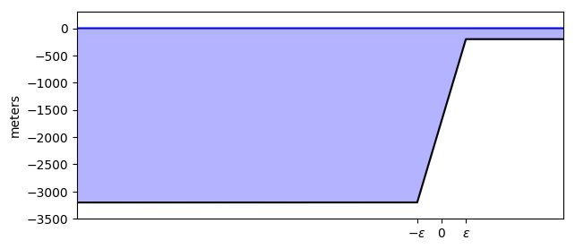
Figure 1: Bathymetry showing deep ocean for $x<-\epsilon$, a linear continental slope for $-\epsilon\leq x\leq\epsilon$, and a continental shelf for $x>\epsilon$.

Green’s Law predicts that the amplitude of a wave moving up a slowly varying slope will be magnified by a factor of

(5) $$C_{G}=(h_{\ell}/h_{r})^{1/4}.$$

This is valid if the wavelength of the wave is significantly smaller than the width $2\epsilon$ of the slope. For the examples, we use $h_{\ell}=3200$ m and $h_{r}=200$ m, which are realistic values and were chosen to have a ratio of 16, so that $C_{G}=2$.

To illustrate the shoaling behavior of waves governed by the shallow water equations, in Figs. 3 and 3 we show the solution to these equations when the initial conditions consist of a square pulse wave approaching a continental slope with three different choices of the continental slope. Although a square pulse is not a realistic tsunami, for the linear equations over flat bathymetry examining this case is very useful to help explain the behavior of the solution as the slope is made more steep. A square pulse can be viewed a pair of discontinuities (a positive jump followed by a negative jump), and we will first study the case of a single jump discontinuity propagating toward the shelf. We can then use the superposition of two such solutions to explain the behavior of the square pulse, giving insight also into the shoaling behavior of a more general wave.

Figure 3 shows a case in which a square pulse moves up a slope that is broad relative to the width of the pulse, a case where Green’s Law should approximately apply. The initial surface displacement is shown on the left, and consists of a pulse with amplitude $A=1$ m, and with fluid velocity $u=\sqrt{g/h_{\ell}}$ in the pulse, to give a purely right-going wave (based on the eigenvectors). The plot on the right shows the solution at a later time when the wave has been amplified due to shoaling by roughly the expected factor of $C_{g}=2$. The pulse also becomes narrower as the wave speed decreases. There is a very small amplitude reflected wave in this case, too small to be seen in the plot. There is also a bit of a negative tail following the transmitted pulse that we will say more about later.

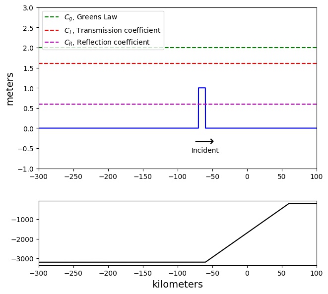
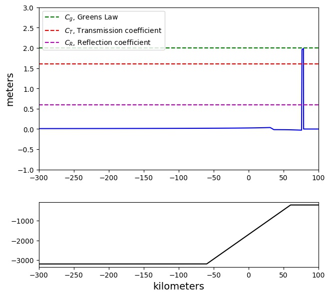
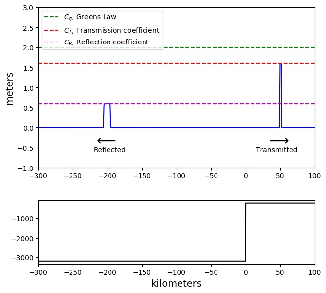
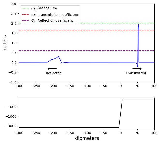
Figure 2: Left: The initial data consists of a square pulse of width 10 km and height 1 m propagating to the right toward a continental slope with $\epsilon=60$ km. Right: Solution at a later time $t=1500$ seconds, when the pulse has become narrower and taller on the shelf, with very little reflected energy. The amplitude is close to that predicted by Green’s Law. The bottom plots show the bathymetry, with a different vertical scale.

Figure 3: Left: Solution when the smooth continental slope of Fig. 3 has been replaced with a sharp discontinuity. The solution at $t=1500$ now consists of a right-going transmitted pulse on the shelf and a left-going reflected pulse in the ocean. The initial pulse width is again 10 km. Right: Solution with a steep slope ($\epsilon=5$ km), showing more reflected energy than in the case shown in Fig. 3.

Figure 3 shows solutions to the equations with the same initial conditions as in Fig. 3 but on steeper slopes. In the left figure, the slope is replaced by a jump discontinuity at $x=0$. In this case Green’s Law does not hold. Instead, the incident pulse is partially transmitted as a narrower pulse with height $C_{T}A$ and partially reflected as a left-moving wave with height $C_{R}A$. Using the eigenvectors to the left and right of $x=0$ and continuity of the solution, we can derive the standard transmission and reflection coefficients (see Section 2):

(6) $$C_{T}=\frac{2\sqrt{h_{\ell}}}{\sqrt{h_{\ell}}+\sqrt{h_{r}}},\qquad C_{R}=\frac{\sqrt{h_{\ell}}-\sqrt{h_{r}}}{\sqrt{h_{\ell}}+\sqrt{h_{r}}}=C_{T}-1.$$

With our choice of $h_{\ell}$ and $h_{r}$ we have $C_{T}=1.6$ and $C_{R}=0.6$.

Finally, the right side of Fig. 3 shows a case where the width of the continental slope is comparable to the width of the incoming pulse. In this case the solution is more complicated, consisting of a transmitted wave on the shelf that has a peak value close to that predicted by Green’s Law but decreasing behind the peak and has a negative tail, along with a reflected wave with complicated structure. As the slope is made more broad, the amplitude of the reflected wave will decrease and eventually go to zero in the Green’s Law limit. Our goal is to fully describe waves in this transitional regime of steep slopes and the manner in which this reflection disappears. In Section 4 we illustrate that realistic tsunamis can fall into this transitional region, suggesting that a better understanding of this case is important in practice.

1.3 Transmission of mass and of energy

First we note that Green’s Law applies to the amplitude of waves, not to their mass or energy. Of course the mass of water is conserved and so $\int_{-\infty}^{\infty}(h(x)+\eta(x,t))\,dx$ is constant in time. Moreover from this or directly from the first conservation law of (1) we see that the “wave mass” $\bar{\eta}\equiv\int_{-\infty}^{\infty}\eta(x,t)\,dx$ is constant in time and always equal to the initial wave mass. Similarly, the second conservation law of (1) shows that $\bar{u}\equiv\int_{-\infty}^{\infty}u(x,t)\,dx$ is constant in time. Suppose the initial data is identically 0 for $x>-\epsilon$ and consists of some purely right-going wave with finite mass $\bar{\eta}$ travelling over the deep ocean. Then $u(x,0)=\sqrt{g/h_{\ell}}\,\eta(x,0)$ for all $x$, and so $\bar{u}=\sqrt{g/h_{\ell}}\,\bar{\eta}$. For large times, the solution approaches 0 over the continental slope region, and consists of a purely left-going reflected wave and a purely right-going transmitted wave. Thus for sufficiently large $t$ we can decompose $\eta(x,t)=\eta^{R}(x,t)+\eta^{T}(x,t)$, and similarly for $u$, where we have $\eta^{R}(x,t)\equiv 0$ for $x>-\epsilon$ and $u^{R}(x,t)=-\sqrt{g/h_{\ell}}\,\eta^{R}(x,t)$ for all $x$, while $\eta^{T}(x,t)\equiv 0$ for $x<\epsilon$ and $u^{T}(x,t)=\sqrt{g/h_{r}}\,\eta^{T}(x,t)$ for all $x$. If we define $\bar{\eta}^{R}=\int_{-\infty}^{\infty}\eta^{R}(x,t)\,dx=\int_{-\infty}^{-\epsilon}\eta(x,t)\,dx$ and $\bar{\eta}^{T}=\int_{-\infty}^{\infty}\eta^{T}(x,t)\,dx=\int_{\epsilon}^{\infty}\eta(x,t)\,dx$, then by conservation of $\eta$ and $u$, we obtain a linear system of two equations

(7) $$\begin{split}\bar{\eta}^{R}+\bar{\eta}^{T}&=0,\\ -\sqrt{g/h_{\ell}}\,\bar{\eta}^{R}+\sqrt{g/h_{r}}\,\bar{\eta}^{T}&=\sqrt{g/h_{\ell}}\,\bar{\eta},\end{split}$$

which can be solved to find that the total reflected and transmitted mass are given respectively by

(8) $$\begin{split}\bar{\eta}^{R}&=\frac{\sqrt{h_{\ell}}-\sqrt{h_{r}}}{\sqrt{h_{\ell}}+\sqrt{h_{r}}}\eta^{0}\equiv\bar{C}_{R}\bar{\eta},\\ \bar{\eta}^{T}&=\frac{2\sqrt{h_{r}}}{\sqrt{h_{\ell}}+\sqrt{h_{r}}}\equiv\bar{C}_{T}\bar{\eta}.\end{split}$$

Note that $\bar{C}_{T}=\sqrt{h_{r}/h_{\ell}}\,C_{T}$. As the pulse passes over a discontinuous jump in bathymetry, the amplitude increases by $C_{T}$ but its width decreases by $\sqrt{h_{r}/h_{\ell}}$ due to the change in wave speed, and so its mass changes by the product of these, which is $\bar{C}_{T}$. The reflected wave, on the other hand, has the same width as the incident pulse, and so $\bar{C}_{R}=C_{R}$.

The transmission and reflection coefficients for mass from (8) apply regardless of the width of the continental slope, and in fact are the same for any specified variation of $h(x)$ provided it varies only over a finite region and is identically equal to $h_{\ell}$ and $h_{r}$ away from the slope. They are also independent of the shape of the pulse $\eta(x,0)$ as long as the initial wave is purely right-going, $u(x,0)=\sqrt{g/h_{\ell}}\eta(x,0)$, and $\eta(x,0)=0$ for $x>-\epsilon$.

Note that the square pulse shown in Fig. 3 for a very broad continental slope also appears to be transmitted as a square pulse, and the change in wave speed again suggests the width of the pulse will be reduced by $\sqrt{h_{r}/h_{\ell}}$. But if the initial amplitude is $A$ then the amplitude of the transmitted wave is close to $C_{G}A$ rather than $\bar{C}_{T}A$, and so it seems that too much mass has been transmitted onto the shelf. However, recall that there is also a small negative trailing wave. It turns out this wave has amplitude that decreases as the width of the continental slope increases, while at the same time it spreads out farther, in such a way that its total mass is constant and roughly equal to $(\bar{C}_{T}-C_{G})A<0$, which cancels the excess mass that appears in the transmitted pulse.

It is interesting to consider the case of a localized variation in bathymetry, with $h_{r}=h_{l}$ and any variations restricted to $-\epsilon<x<\epsilon$, e.g., an underwater ridge or sill. Then $\bar{C}_{R}=0$ and $\bar{C}_{T}=1$, so the total mass reflected is zero while the transmitted mass is equal to the mass of the original wave. This does not mean, of course, that the transmitted wave has the same form as the incident wave, nor that there are no reflections (only that the integral of the reflected wave vanishes).

It is also interesting to note that the total energy propagated onto the shelf varies as the width of the slope or the initial pulse are varied. A wave that is purely left-going or right-going satisfies equipartition of energy between potential and kinetic energy (see e.g. [2]), so it suffices to consider, for example, the potential energy given by $E(x,t)=\rho g\int_{-\infty}^{\infty}\eta^{2}(x,t)\,dx.$ where $\rho$ is the density of water (which is assumed to be constant in this calculation). Consider the case of a step function continental slope and an initial pulse of height $A$ and width $w$, for which $E(x,0)=\rho gwA^{2}$. The reflected wave has height $C_{R}A$ and width $w$, while the transmitted wave has height $C_{T}A$ and width $w\sqrt{h_{r}/h_{\ell}}$. So the total potential energy is $\rho g(C_{R}^{2}w+C_{T}^{2}w\sqrt{h_{r}/h_{\ell}})A^{2}=\rho gwA^{2}$, illustrating conservation of energy. For a very broad slope, for which Green’s Law holds, the energy in the reflected wave goes to zero (even though its mass is constant, it becomes more spread out with smaller amplitude as the width of the continental slope increases, and the energy is quadratic in $\eta$, so this integral vanishes). The transmitted wave carries all of the energy; it has height $C_{G}A$ and width $w\sqrt{h_{r}/h_{\ell}}$, and hence energy $\rho gC_{G}^{2}w\sqrt{h_{r}/h_{\ell}}A^{2}=\rho gwA^{2}$.

2 A single jump discontinuity as the approaching wave

To better understand the way in which the waves deform in the intermediate case between Green’s law and pure reflection and transmission, consider the case of a single jump discontinuity in the initial data together with the piecewise linear bathymetry (4). As data we take

(9) $$\eta(x,0)=\begin{cases}A,&x<-\epsilon,\\ 0,&x\geq-\epsilon\end{cases},\qquad u(x,0)=\begin{cases}\sqrt{g/h_{\ell}},&x<-\epsilon,\\ 0,&x\geq-\epsilon\end{cases}.$$

This can be viewed as a right-going hydraulic jump (or bore) moving across the ocean, at the instant when it first encounters the continental slope, as shown in the $t=0$ plot in Fig. 5.

If $\epsilon=0$ (a jump discontinuity in bathymetry, at the same point as the jump in the initial data), then the problem has the form of a “Riemann problem”. Problems of this nature form the basis for much of the theory of hyperbolic PDEs, and of many numerical methods; see e.g. Chap. 9 of [11] for more discussion of this particular Riemann problem and its solution. The initial jump in $(\eta,u)$ splits into a single left-going wave across which $\eta$ jumps from $\eta_{\ell}$ to some state $\eta_{m}$, and a single right-going wave across which $\eta$ jumps from $\eta_{m}$ to $\eta_{r}$. There is a single intermediate state $\eta_{m}$ since the solution must be continuous at $x=0$. Similarly, the Riemann solution must have a single intermediate state $u_{m}$. Moreover, due to the form of the eigenvectors displayed in Eq. 3, across the left-going wave we must have $(u_{m}-u_{\ell})=-\sqrt{g/h_{\ell}}\,(\eta_{m}-\eta_{\ell})$, while across the right-going wave $(u_{r}-u_{m})=\sqrt{g/h_{r}}\,(\eta_{r}-\eta_{m})$. These conditions result in a system of two equations that, for the initial data (9), yield $\eta_{m}=C_{T}A$ and $\eta_{m}-\eta_{\ell}=C_{R}A$, with $C_{T}$ and $C_{R}$ given by (6).

For any $\epsilon>0$, the solution behaves differently than in the singular case of a discontinuous continental slope. As the bore moves up the smooth slope it amplifies and also generates a reflected wave. Denote the solution to this problem by $(\eta^{[\epsilon]}(x,t),u^{[\epsilon]}(x,t))$ to indicate that this solution depends on the parameter $\epsilon$ defining the width of the continental slope. It is easy to check from the equations (1) that the solution scales with $\epsilon$ in the following manner: if we calculate the solution $(\eta^{[1]},u^{[1]})$ for $\epsilon=1$ then for any other value $\epsilon>0$ we have:

(10) $$\eta^{[\epsilon]}(x,t)=\eta^{[1]}(x/\epsilon,t/\epsilon),\qquad u^{[\epsilon]}(x,t)=u^{[1]}(x/\epsilon,t/\epsilon).$$

Figure 5 shows the form of this solution, as computed using Clawpack [3] on a very fine grid. Below we will derive the main features of this solution.

As the bore moves up the continental slope to some point $x>-\epsilon$, its amplitude increases according to Green’s Law to $(h(x)/h_{\ell})^{1/4}A$, based on the depth $h(x)$ at the point the bore has reached and the initial depth $h_{\ell}$ (this is not obvious, but will be justified below in section 3.2). Upon reaching the shelf at $x=\epsilon$, it has reached an amplitude $C_{G}A=(h_{r}/h_{\ell})^{1/4}A$, and is followed by a decrease in amplitude down to the value $C_{T}A$ given by the transmission coefficient (6). As it propagates up the shelf, it also gives rise to a left-going wave that increases to just above $C_{T}A$ before settling down to the value $C_{T}A$. This reflected wave thus has overall amplitude $C_{T}A-A=C_{R}A$.

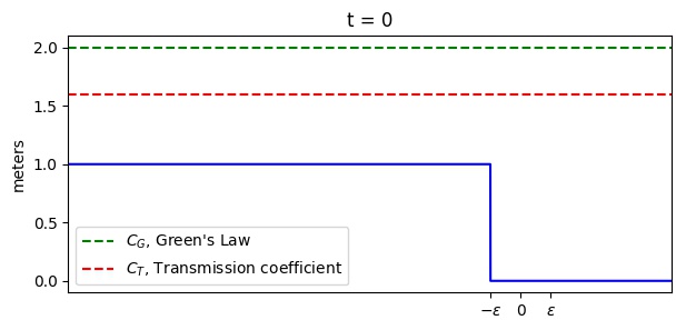
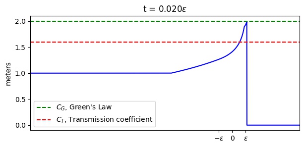
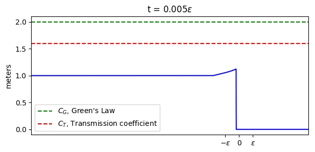
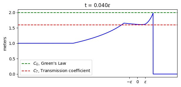
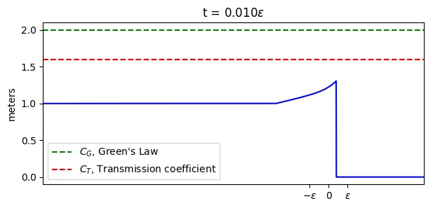
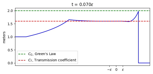
Figure 4: Left column: Initial data $\eta^{[\epsilon]}(x,0)$ at $t=0$, and evolution to $t=0.01\epsilon$, where $\epsilon$ is the half-width of the continental slope. Right column: Further evolution to $t=0.07\epsilon$ seconds (when $\epsilon$ is in meters). At later times the left going and right-going waves propagate outward over constant bathymetry with no further change in shape.

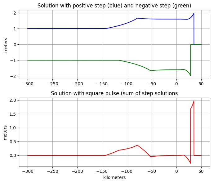
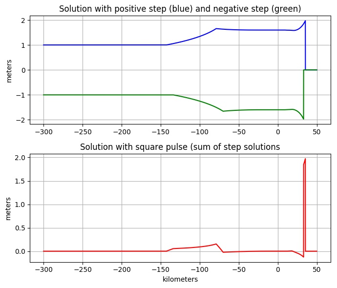
Figure 5: The solution to the shoaling problem with square pulse initial data can found as the linear combination of the single bore solution and a shifted and negated version of the single bore solution. (a) A wider pulse has a larger shift between the two. (b) A narrower pulse has a smaller shift between the two, more cancellation of the reflected waves, and a transmitted pulse that more closely resembles the Green’s Law prediction.

Below we will explore some details of this solution $\eta^{[\epsilon]}(x,t)$, but first we note that once we have observed the form of this solution, it is easy to understand the results shown in Figs. 3 and 3 and the transition between them. The square pulse initial data considered in Section 1 can be viewed as a jump discontinuity from $\eta=0$ up to $\eta=A$ initially located at $x=\epsilon$, followed by another jump discontinuity from $\eta=A$ back down to $\eta=0$ initially located at $x=\epsilon-w$, where $w$ is the width of the square wave. The solution for each of these initial conditions has the form discussed above, and the full solution for the pulse is hence (by linearity) the sum of the solutions for each jump separately. Figure 5 shows each of these solutions separately on the top, and the sum of the two on the bottom. These are shown for two different choices of the width $w$ of the initial pulse. As the width decreases, the two waves cancel out almost everywhere except near the initial peak location, where the amplitude jumps up to $C_{G}A$. Hence in the limit of a narrow pulse relative to the width $\epsilon$ of the continental slope ($w/\epsilon\rightarrow 0$), we recover the Green’s Law limit of a pulse with amplitude $C_{G}A$. For larger values of $w/\epsilon$ there is less cancellation of the left-going waves and a larger apparent reflected wave.

But note that for any values of $w$ and $\epsilon$, the total mass of the reflected wave is $wC_{R}A$, as expected from our earlier discussion. We can approximate

(11) $$\begin{split}\eta(x,t)&=\eta^{[1]}(x/\epsilon,t/\epsilon)-\eta^{[1]}((x-w)/\epsilon,t/\epsilon)\\ &\approx(w/\epsilon)\eta^{[1]}_{x}(x/\epsilon,t/\epsilon).\end{split}$$

The amplitude vanishes as $w/\epsilon\rightarrow 0$, while integrating this over the left-going wave shows that the reflected mass

(12) $$\begin{split}\int_{-\infty}^{-\epsilon}\eta(x,t)\,dx&\approx(w/\epsilon)\int_{-\infty}^{-\epsilon}\eta^{[1]}_{x}(x/\epsilon,t/\epsilon)\,dx\\ &=w(\eta_{m}-\eta_{\ell})\\ &=wC_{R}A.\end{split}$$

remains constant if $w$ is fixed, independent of $\epsilon$.

3 Interpretation as a layered medium with piecewise constant bathymetry

A smooth continental slope can be viewed as the limiting case of a sequence of small jump discontinuities. Piecewise constant bathymetry of this nature defines a “layered medium” in the standard terminology of wave propagation problems; we provide a more general analysis of this case in [6]. To understand the behavior of waves through such a medium, it is natural to first consider a layered medium with only a few intermediate layers. The single jump discontinuity between depths $h_{\ell}$ and $h_{r}$ that we used to define the transmission and reflection coefficients in (6) can be partitioned into $N+1$ discontinuities separating $N$ intermediate layers. Figure 6 shows the bathymetry if there are $N=0,~{}1$ or 2 intermediate layers (top plots) and also shows how a single initial discontinuity of amplitude $A$ propagates in the the $x$–$t$ plane in each case. With no intermediate layer (Fig. 6, $N=0$), the wave splits into transmitted and reflected waves only once, with amplitudes $C_{T}A$ and $C_{R}A$ respectively. With $N=1$ interior layer the solution is already much more complicated, with internal reflections in the layer that result in an infinite sequence of waves eventually departing to both the right and to the left, as shown in Fig. 6. The amplitude of later waves decays rapidly since each reflection coefficient is less than one. We will show in Section 3.1 that the first wave departing to the right (after transmission through each layer and no reflection) has amplitude greater than $C_{T}A$, but that subsequent departing waves (with 2, 4, 6, or more internal reflections) also affect the value of $\eta$ and asymptotically they sum to $C_{T}A$. Similarly, the reflections that depart from the left (after 1, 3, 5, or more reflections) all sum to $C_{R}A$.

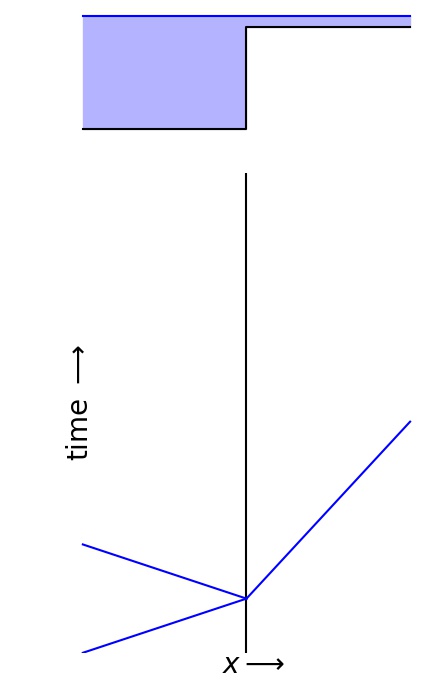
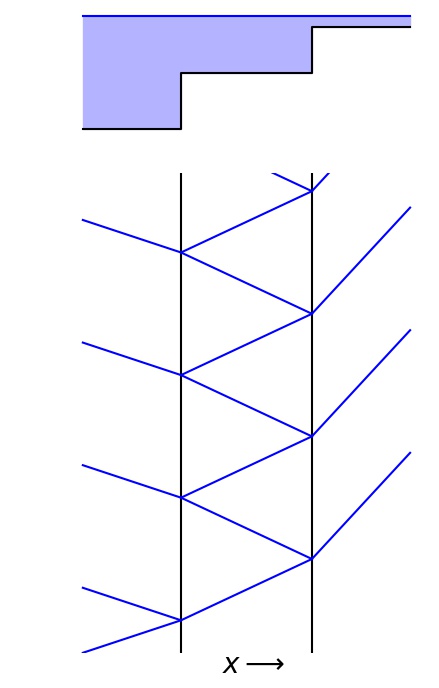
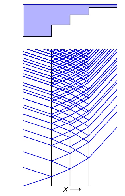
Figure 6: Plots in the $x$–$t$ plane showing an initial right-going wave interacting with a layered medium (i.e.  bathymetry with jump discontiuities, as shown at the top of each plot). (a) With a single interface, where only one transmitted and reflected wave are generated. (b) With two interfaces and a single intermiate layer. (c) With three interfaces and two intermediate layers.

When the same jump from $h_{\ell}$ to $h_{r}$ is split into three discontinuities, as shown in Fig. 6, then there are many more internal reflections but the same asymptotic limits still hold, as shown in Section 3.1. When additional layers are added, these asymptotic results continue to hold (see [6]). Moreover, the first transmitted wave exiting to the right (with no internal reflections) asymptotes to magnitude $C_{G}A$ as the number of layers increases, where $C_{G}$ is the value predicted by Green’s Law. This can be shown analytically; see Section 3.2.

In fact, the full wave form of $\eta^{[\epsilon]}(x,t)$ can be worked out from asymptotic limits of the multilayer case by considering all internal reflections and transmissions as $N\rightarrow\infty$. However, the number of waves that must be considered grows exponentially in $N$. We present this more complicated analysis in [6]. Here we only discuss two illuminating special cases: a single internal layer and the first transmitted wave in the limit of infinitely many layers.

3.1 Single intermediate layer

We derive some results on wave propagation through a layered medium for the case of a single intermediate layer, as shown in in Fig. 6 where the intermediate step in bathymetry has depth $h_{m}$ with $h_{r}<h_{m}<h_{\ell}$. Define the following transmission coefficients:

(13) $$C_{T}^{\ell m}=\frac{2\sqrt{h_{\ell}}}{\sqrt{h_{\ell}}+\sqrt{h_{m}}},\quad C_{T}^{mr}=\frac{2\sqrt{h_{m}}}{\sqrt{h_{m}}+\sqrt{h_{r}}},\quad C_{T}^{m\ell}=\frac{2\sqrt{h_{m}}}{\sqrt{h_{\ell}}+\sqrt{h_{m}}},$$

where for example the superscript $mr$ indicates transmission of a right-going wave from the middle layer to the right layer, and $m\ell$ indicates transmission of a left-going wave from the middle layer to the left layer. Similarly define the reflection coefficients for internal reflections in the intermediate layer as

(14) $$C_{R}^{mr}=\frac{\sqrt{h_{m}}-\sqrt{h_{r}}}{\sqrt{h_{m}}+\sqrt{h_{r}}},\quad C_{R}^{m\ell}=\frac{\sqrt{h_{m}}-\sqrt{h_{\ell}}}{\sqrt{h_{m}}+\sqrt{h_{\ell}}}$$

Then an initial right-going wave consisting of a discontinuity in $\eta$ of amplitude $A$ leads to a first transmitted wave of amplitude $C_{T}^{\ell m}C_{T}^{mr}A$. This is larger than $C_{T}A$, where $C_{T}$ is the transmission coefficient with no intermediate layer from (6), but not as large as $C_{G}A$, the value found in Section 3.2 for a smooth transition. This first wave is followed by transmitted waves that have undergone $2n$ internal reflections for $n=1,~{}2,~{}3,~{}\ldots$, each of which has amplitude

(15) $$C_{T}^{\ell m}(C_{R}^{mr}C_{R}^{ml})^{n}C_{T}^{mr}A.$$

Note that $-1<C_{R}^{mr}C_{R}^{ml}<0$ and so the sum of all the transmitted waves, including the first wave with no reflections, is given by the geometric series

(16) $$\sum_{n=0}^{\infty}C_{T}^{\ell m}(C_{R}^{mr}C_{R}^{ml})^{n}C_{T}^{mr}A=\left(\frac{C_{T}^{\ell m}C_{T}^{mr}}{1-C_{R}^{mr}C_{R}^{ml}}\right)A=C_{T}A$$

As expected, the state behind the right-going waves decays to the same state $C_{T}A$ obtained behind the right-going transmitted wave in the case of no interior layers.

Similarly, the sum of all left-going waves that depart into the deep ocean after $2n+1$ internal reflections (for $n=0,~{}1,~{}2,~{}\cdots$) is given by

(17) $$\sum_{n=0}^{\infty}C_{T}^{\ell m}C_{R}^{mr}(C_{R}^{ml}C_{R}^{mr})^{n}C_{T}^{m\ell}A=C_{R}A,$$

where $C_{R}$ is the reflection coefficient in the case of no intermediate layers. But note that there is a time lag between each departing wave, so the composite reflected wave takes the form of a step function with infinitely many jumps that decay exponentially with $n$.

3.2 Infinitely many layers and the first transmitted wave

We now consider the amplification of the wave as it is transmitted through each interface of a layered medium, ignoring all the reflected waves generated in the process. The final amplitude of this “first transmitted wave” will be denoted by $C_{T}^{f}A$, and we will show that $C_{T}<C_{T}^{f}<C_{G}$ and that this transmission coefficient asymptotes to the Green’s Law coefficient $C_{G}$ as the number of layers increases. A different approach to deriving this same result is taken in [6] and [5], where more general results are derived for the waves that also experience internal reflections.

The amplitude of the first transmitted wave in the case of a single intermediate layer can be represented by $A_{t_{1}t_{2}}$, signifying transmission through the first and second interface:

(18) $$A_{t_{1}t_{2}}=C_{T}^{\ell m}C_{T}^{mr}A=\frac{2\sqrt{h_{\ell}}}{\sqrt{h_{m}}+\sqrt{h_{\ell}}}\frac{2\sqrt{h_{m}}}{\sqrt{h_{m}}+\sqrt{h_{r}}}A.$$

In the case of two intermediate layers, the amplitude of the first transmitted wave is given by

(19) $$A_{t_{1}t_{2}t_{3}}=\frac{2\sqrt{h_{\ell}}}{\sqrt{h_{m_{1}}}+\sqrt{h_{\ell}}}\frac{2\sqrt{h_{m_{1}}}}{\sqrt{h_{m_{1}}}+\sqrt{h_{m_{2}}}}\frac{2\sqrt{h_{m_{2}}}}{\sqrt{h_{m_{2}}}+\sqrt{h_{r}}}A.$$

It can be seen that $A_{t_{1}t_{2}t_{3}}$ is larger than $A_{t_{1}t_{2}}$ and that increasing the number of layers increases the amplitude of the first transmitted wave.

More generally, consider piecewise constant bathymetry with $N$ intermediate steps having depths $h_{i}$ chosen with $h_{i}=h_{\ell}+i\Delta h$ where $\Delta h=(h_{r}-h_{\ell})/N$ for $i=1,~{}2,~{}\ldots,~{}N$. We also define $h_{0}=h_{\ell}$ and $h_{N+1}=h_{r}$. Then the transmission coefficient at the interface between $h_{i}$ and $h_{i+1}$ is given by

$$C_{T}^{i}=\frac{2\sqrt{h_{i}}}{\sqrt{h_{i}}+\sqrt{h_{i}+\Delta h}}=\frac{2}{1+\sqrt{1+\frac{\Delta h}{h_{i}}}}.$$

This allows us to find the continuous limit of the leading amplitude by considering the scenario with infinitely many layers. The amplitude of the first transmitted wave would then be given by

(20) $$\lim_{N\to\infty}\prod_{i=0}^{N}C_{T}^{i}A=\lim_{N\to\infty}\prod_{i=0}^{N}\bigg{(}\frac{2}{1+\sqrt{1+\frac{\Delta h}{h_{i}}}}\bigg{)}A\equiv C_{T}^{f}A,$$

Taking the log of $C_{T}^{f}$ converts the infinite product into a sum,

(21) $$\log(C_{T}^{f})=\lim_{N\to\infty}\sum_{i=0}^{N}\log\bigg{(}\frac{2}{1+\sqrt{1+\frac{\Delta h}{h_{i}}}}\bigg{)}.$$

Using the Taylor expansion then results in

(22) $$\log(C_{T}^{f}) =-\lim_{N\to\infty}\sum_{i=0}^{N}\bigg{(}\frac{\Delta h}{4h_{i}}-\frac{\Delta h^{2}}{16h_{i}^{2}}+\ldots\bigg{)}.$$

Since the sum of the $\Delta h^{2}$ and higher order terms vanish in the limit, we obtain

(23) $$\log(C_{T}^{f})=-\lim_{N\to\infty}\frac{h_{r}-h_{\ell}}{N}\sum_{i=0}^{N}\frac{1}{4h_{i}}.$$

This sum approaches an integral in the limit, giving

(24) $$\log(C_{T}^{f})=-\int_{h_{\ell}}^{h_{r}}\frac{1}{4x}dx=-\frac{1}{4}\log\bigg{(}\frac{h_{r}}{h_{\ell}}\bigg{)}$$

and hence

(25) $$C_{T}^{f}=(h_{\ell}/h_{r})^{1/4}.$$

This is exactly the Green’s Law coefficient $C_{G}$ from Eq. 5, showing that the first transmitted wave has amplitude $C_{G}A$ in the limit as the number of internal layers goes to infinity, i.e. as the step function bathymetry is smoothed out to a continuous continental slope. Note also that this argument is independent of the locations $x_{i}$ corresponding to each jump discontinuity from $h_{i}$ to $h_{i+1}$, and so the same result holds regardless of whether we discretize a narrow or wide slope, and regardless of the shape of the slope; it need not be a discretization of a linear slope of the sort shown in Fig. 1.

4 Implications for real tsunamis

Both Green’s Law and the more general theory presented here are based on the one-dimensional shallow water equations and would apply to a real tsunami only if it were a plane wave approaching a continental shelf in the normal direction, in a case where the shelf is invariant in the along-shore direction. A real tsunami is typically a complex wave train by the time it reaches a shelf, and is not necessarily approaching normal to the shore. Moreover, the continental shelf varies greatly over relatively short spatial scales, with undulations in width and sometimes deep valleys or outcroppings that will focus or defocus the approaching waves. Predicting the amplitude of the wave hitting the beach from the amplitude seaward of the shelf is generally not possible with any precision using one-dimensional theory alone, and simulations in two spatial dimensions with the appropriate shelf bathymetry and approaching wave train should be used for detailed inundation predictions.

Nonetheless, one-dimensional theory is still often used to get an estimate of the amplitudes along a coastline, particularly in cases where many tsunamis must be simulated and nearshore amplitudes estimated over a large region of interest, for example in global probabilistic hazard assessment, e.g. [12], [13], [16]. Hence we believe it is important for practitioners to understand the implications of the results presented here.

Comparing this theory with a real tsunami is difficult because each tsunami and shelf bathymetry is unique. Here we simply show one example. We have attempted to identify a case where the leading tsunami wave is relatively planar and normal to the coast and the width of the continental slope is comparable to the width of the tsunami, where the results of this paper imply that amplification should be less than what Green’s Law predicts.

Figure 7 shows a simulation of the tsunami arising from the 2011 Great East Japan earthquake (also known as the Tohoku event), performed with the GeoClaw software [3] using an earthquake source model provided by the NOAA Center for Tsunami Research and recently used in a comparison study with tide gauge observations for this event [1]. This seafloor deformation file along with the GeoClaw code used to produce these figures is available in the code archive for this paper [7].

Figure 7 also shows the leading wave of this tsunami as it is approaching the coast of Oregon. Black contours of bathymetry show the continental shelf and red contours show the wave elevation. Figure 7 shows the wave approaching the shelf, where it is roughly planar with a fairly uniform amplitude of about 0.15 m. Figure 7 shows the wave 25 minutes later, after passing onto the shelf. The wave has amplified by varying amounts. The broader shelf around latutude 44.2 causes a folding in of the wave along this latitude (due to the slower wave speed on the shallow shelf) and amplification along this latitude and lower amplitudes to the north and particularly to the south (e.g., along latitude 44.0).

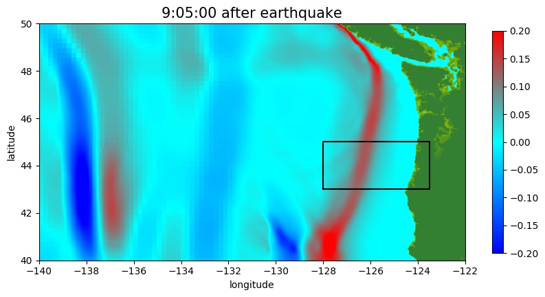
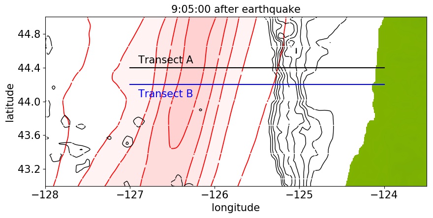
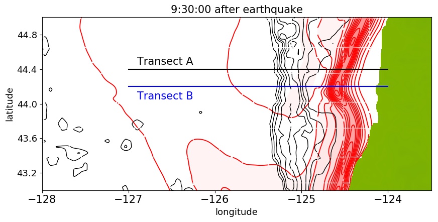
Figure 7: (a) Portion of a simulation of the 2011 Tohoku Tsunami, 9:05 hours after the earthquake as the leading wave is approaching the west coast of North America. The black rectangle indicates the region shown in the other two plots. (b) Zoom on the wave approaching the central Oregon Coast. The black contours show the topograph of the continental slope (contours at depths of $300,~{}600,~{}\ldots,~{}2700$ m. Red contours and shading show surface elevation above sea level, with contours at $0.025,~{}0.5,~{}\ldots,~{}0.5$ m. (c) Zoom at a later time 9:30 hours post-quake, after the wave has passed onto the continental shelf. Two transects are also indicated, along which vertical cross-sections of the bathymetry and tsunami are shown in Fig. 8.

In Fig. 8 we show transects of the bathymetry and of the solution along two transects, one at latitude 44.4, where the amplitude is roughly equal to the mean amplitude around this region, and one at latitude 44.2, where geometric focusing from the shelf geometry causes greater amplification. Even in the latter case we see that the wave amplification as it first passes onto the shelf is less than what is predicted by Green’s Law, which is indicated by the dashed green curve. The solution is shown at three times along each transect, and the red solid line also shows the maximum sea surface at each point over the full time range from 9:00 to 9:50 hours after the earthquake, showing the amplification as the wave goes on to the shelf. The Green’s Law value at each point $x$, based on the depth $h(x)$ at this point relative to the roughly uniform 3000 m depth seaward of the shelf. The blue dashed line at each $x$ shows the amplification that would be predicted by the transmission coefficient from the deep ocean to depth $h(x)$, if the shelf were replaced by a step discontinuity up to the shelf depth at this location.

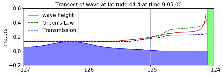
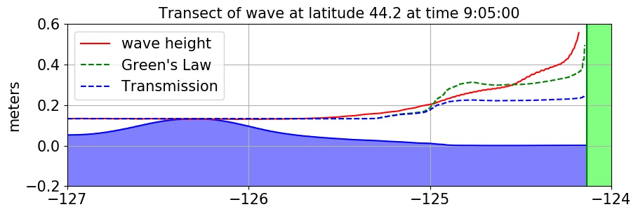
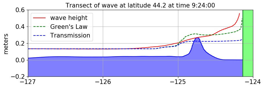
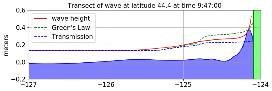
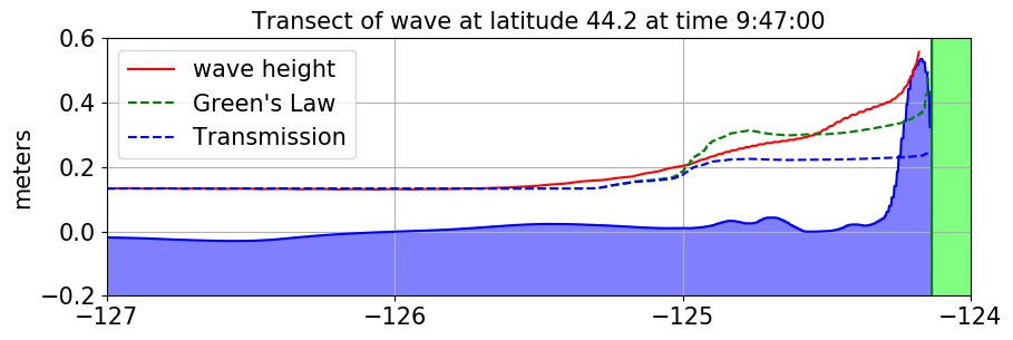
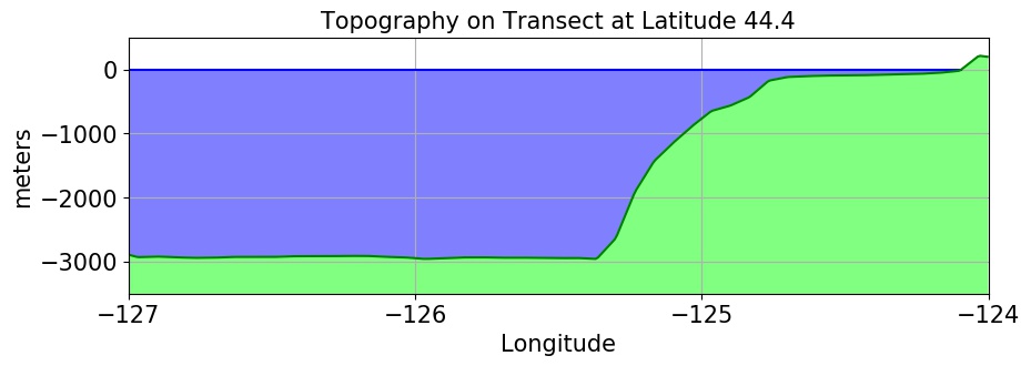
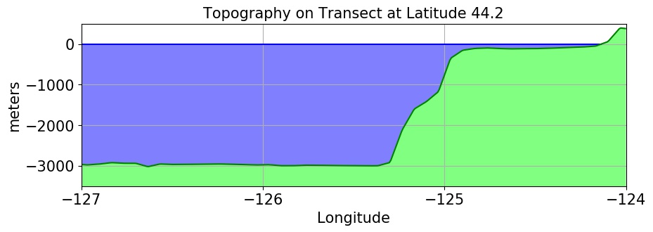
Figure 8: Vertical cross sections of the solution from Fig. 7 (and bathymetry in the bottom plot) along two different transects. Left column: Transect A at latitude 44.4^∘N, Right column: Transect B at latitude 44.2^∘N. See the text for discussion of the curves shown.

Based on the theory in this paper, we expect the wave to be amplified by more than the transmission coefficient defined above, but by less than Green’s Law would suggest. Indeed we see that the red curve of maximum amplitude lies between the two dashed curves over most of the shelf at latitude 44.4 and at least initially as the wave moves onto the shelf at latitude 44.2. As the wave moves into much shallower water near the shore, Green’s Law roughly applies to predict further amplification from the shelf depth to the nearshore depth, and we see that the actual wave amplitude grows even faster near shore due to local bathymetry effects and runup of the relatively broad wave. At latitude 44.2 additional amplification is observed due to the shelf geometry.

5 Conclusions

Green’s Law is often used to estimate the amplification of tsunamis as they pass from the deep ocean onto a continental shelf. This is a good approximation if the continental slope is sufficiently gentle that the width of the slope region is large compared to the wavelength. For steeper slopes there is less amplification and more reflection of waves, asymptoting to values given by the transmission and reflection coefficient for a sharp interface. Many realistic tsunami applications fall in the intermediate region, as illustrated for the 2011 Tohoku earthquake tsunami approaching the Oregon coast in Section 4.

We have presented a mathematical analysis of the intermediate behavior that provides new understanding of the connection between the two limiting cases. In Section 2 we showed that for a wave consisting of a right-going jump discontinuity approaching a linear slope, there is a solution that varies in a self-similar manner as the width of the continental slope is varied. Viewing a square pulse as a linear superposition of two such waves shows the manner in which the reflected amplitude and energy decays as the slope width increases, even though the the reflected mass is independent of the slope width. Approximating a continuous slope as a piecewise constant “layered medium”, as done in Section 3, shows that the “first transmitted wave” satisfies Green’s Law but that the sum of all transmitted an reflected waves agree with the transmission and reflection coefficients obtained from a single sharp interface.

Additional mathematical analysis that gives a more complete description of the solution, also in the more general case of a linear wave equation media for which the wave speed and impedance can very independently, can be found in our companion paper [6]. The numerical experiments shown in this paper were produced using the Clawpack software [3], with code that is available at [7].

Acknowledgements. The authors are grateful to Avi Schwarzschild for stimulating discussions in the early phase of this project.

References

- [1] L. M. Adams and R. J. LeVeque, GeoClaw Model Tsunamis Compared to Tide Gauge Results – Final Report. http://hdl.handle.net/1773/41886, 2017.
- [2] M. J. Berger, D. L. George, and R. J. LeVeque, Adaptive mesh refinement techniques for tsunamis and other geophysical flows over topography, Acta Numerica, (2011), pp. 211–289.
- [3] Clawpack Development Team, Clawpack software, 2017, https://doi.org/10.5281/zenodo.1405834, http://www.clawpack.org. Version 5.5.0.
- [4] A. Dzvonkovskaya, M. Heron, D. Figueroa, and K. Gurgel, Observations and theory of a shoaling tsunami wave, in 2014 Oceans - St. John’s, 2014, pp. 1–5, https://doi.org/10.1109/OCEANS.2014.7003236.
- [5] J. D. George, Green’s law and the Riemann problem in layered media, master’s thesis, University of Washington, 2018.
- [6] J. D. George, D. I. Ketcheson, and R. J. LeVeque, A characteristics-based approximation for wave scattering from an arbitrary obstacle in one dimension. To appear soon on the arXiv, 2019.
-
[7]
J. D. George, D. I. Ketcheson, and R. J. LeVeque, Code to accompany
this paper.
https://github.com/rjleveque/shoaling_paper_figures, 2019. - [8] G. Green, On the motion of waves in a variable canal of small depth and width, Transactions of the Cambridge Philosophical Society, 6 (1838), p. 457.
- [9] S. T. Grilli, R. Subramanya, I. A. Svendsen, and J. Veeramony, Shoaling of Solitary Waves on Plane Beaches, Journal of Waterway, Port, Coastal, and Ocean Engineering, 120 (1994), pp. 609–628, https://doi.org/10.1061/(ASCE)0733-950X(1994)120:6(609).
- [10] M. Heron and A. Dzvonkovskaya, Conceptual view of reflection and transmission of a tsunami wave at a step in bathymetry, in OCEANS 2015 - MTS/IEEE Washington, 2015, pp. 1–4, https://doi.org/10.23919/OCEANS.2015.7404520.
- [11] R. J. LeVeque, Finite Volume Methods for Hyperbolic Problems, Cambridge University Press, 2002, http://amath.washington.edu/~claw/book.html.
- [12] S. Lorito, J. Selva, R. Basili, F. Romano, M. M. Tiberti, and A. Piatanesi, Probabilistic hazard for seismically induced tsunamis: Accuracy and feasibility of inundation maps, Geophysical Journal International, 200 (2015), pp. 574–588.
- [13] F. Løvholt, S. Glimsdal, C. B. Harbitz, N. Zamora, F. Nadim, P. Peduzzi, H. Dao, and H. Smebye, Tsunami hazard and exposure on the global scale, Earth-Science Reviews, 110 (2012), pp. 58–73, https://doi.org/10.1016/j.earscirev.2011.10.002.
- [14] P. A. Madsen, D. R. Fuhrman, and H. A. Schäffer, On the solitary wave paradigm for tsunamis, Journal of Geophysical Research: Oceans, 113 (2008), p. C12012, https://doi.org/10.1029/2008JC004932.
- [15] C. E. Synolakis, Green’s law and the evolution of solitary waves, Physics of Fluids A: Fluid Dynamics, 3 (1991), pp. 490–491, https://doi.org/10.1063/1.858107.
- [16] S. N. Ward and E. Asphaug, Asteroid impact tsunami: A probabilistic hazard assessment, Icarus, 145 (2000), pp. 64–78, http://www.sciencedirect.com/science/article/pii/S0019103599963364.