Symbolic regression in materials science
Abstract
We showcase the potential of symbolic regression as an analytic method for use in materials research. First, we briefly describe the current state-of-the-art method, genetic programming-based symbolic regression (GPSR), and recent advances in symbolic regression techniques. Next, we discuss industrial applications of symbolic regression and its potential applications in materials science. We then present two GPSR use-cases: formulating a transformation kinetics law and showing the learning scheme discovers the well-known Johnson-Mehl-Avrami-Kolmogorov (JMAK) form, and learning the Landau free energy functional form for the displacive tilt transition in perovskite LaNiO3. Finally, we propose that symbolic regression techniques should be considered by materials scientists as an alternative to other machine-learning-based regression models for learning from data.
I Motivation
I.1 Era of big data in materials science
Modern scientists perpetuate the scientific process embodied by the works of Tyco Brahe, Johannes Kepler, and Isaac Newton in the heliocentric revolution. Brahe was the observationalist. He took extensive, precise measurements of the position of planets over time. Kepler was the phenomenologist. From Brahe’s measurements, he derived concise analytical expressions that describe the motion of the solar system in a succinct manner. Last, Newton was the theorist. He realized the mechanism behind the apple falling from the tree is the same as that underlying planets traveling around the sun, which could be formulated into a universal law (Newtonian gravitational law). All three scientific modalities are vital in making scientific discoveries: data acquisition (Brahe), data analysis (Kepler), and derivation from first-principles (Newton).
With recent advances in computer science, theoretical modelling, and experimental instrumentation, materials scientists have in many ways created a “mechanical Brahe” and marched into a new era of big data. Datasets of materials information, obtained from advanced characterization techniquesDeelman et al. (2017); Lupini et al. (2018); Ren et al. (2017), combinatorial experimentsStein et al. (2019); Alberi et al. (2019); Green et al. (2017), high-throughput first-principles simulationsYe et al. (2018); Tanaka et al. (2018), literature miningKim et al. (2017); Krallinger et al. (2017), and other techniques, are created at a faster rate every day with less and less human labor. All of this data enables new opportunities to construct novel laws of phenomenological behavior for systems that previously lacked them.
Inspired by the Materials Genome Initiative (MGI) Government (2014), the materials community is working collaboratively towards making digital materials data accessible to others. Multiple materials databases such as Materials ProjectJain et al. (2013), OQMDSaal et al. (2013), AFLOWLIBCurtarolo et al. (2012), OMDBBorysov et al. (2017), AiiDAPizzi et al. (2016), Citrination and NOMAD, provide public access to millions of materials data points. Accessibility to an immense amount of materials data paves way for the next step of “automating Kepler” in the discovery of governing laws in materials processing-structure-properties-performance relationships, which could advance materials discovery, development, and technology innovation.
Since one of the fundamental research objectives of materials science and engineering is to deliver new materials with optimal performance under specified constraints, it is essential to understand how and which features govern the functionality. In other words, which degrees-of-freedom (or parameters) and their corresponding intrinsic relationships (or dependencies) to the material properties should be optimized. However, the multi-scale nature of materials scienceAlberi et al. (2019), e.g. from atomic-scale crystal structure to complex mesoscale domain structures and bulk mechanical properties or from femotosecond laser probes to hour-long recrystallization reactions, makes it particularly challenging to study many hierarchical relationships of different materials families. Given such a high-dimensional parameter space (e.g. chemical composition, crystal structure, external conditions, etc.), materials scientists often explore a finite subspace of all the factors that govern materials properties and performance. In addition, the available data is typically sparsely distributed. Although, access to a large materials database relieves, in part, the limited-data problem, there is an urgent need for a robust data-processing protocol to help discern governing laws in materials science and to deliver designer materials and synthesis/processing procedures.
I.2 An alternative to machine-learning methods
Much of the burgeoning field of materials informatics focuses on the aforementioned challenges. Machine learning (ML) models are currently the tools of choice for uncovering these physical laws. Although they have shown some promising performance in predicting materials properties Zhuo et al. (2018), typical parameterized machine learning models are not conducive to the next stage of generalizing across domains—the ultimate goal of “automating Newton.”
It is important to note that Newton’s challenge was somewhat made easier, because Kepler’s laws were parsimonious yet predictive. In a modern context, ML models can be predictive but their descriptions are often too verbose (e.g. deep-learning models with thousands of parameters) or mathematically restrictive (e.g. assuming the target variable is a linear combination of input features). Such black-box models have become more prevalent in modern materials science research; however, the interpretability of such models have always been a problem. Although there is a large body of work on data visualization and model understanding to address these issues, those subjects will be out of the scope of this perspective (see Ref. Hall and Gill, 2018 for a review).
In this prospective paper, we focus on an alternative to machine-learning models: symbolic regression. Symbolic regression simultaneously searches for the optimal form of a function and set of parameters to the given problem, and is a powerful regression technique when little if any a-priori knowledge of the data structure/distribution is available.
Figure 1 shows the relative popularity of machine learning and symbolic regression in different research domains. We use data from the “Web of Science Core Collection” database in this analysis web . Among all publications whose topics are related to machine learning or symbolic regression, over 50% of the contributions come from the computer science research community, while multidisciplinary engineering is second. Social science and physical science each makes less than 20% of the contribution to the total number of publications. These two techniques are not so popular in materials science research, as the relative contribution is almost negligible compared to other research domains.
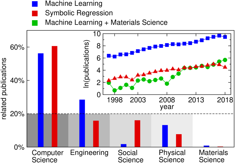
It is not surprising to see a dominant contribution from computer science in both the machine learning and symbolic regression communities, since it is where these techniques were born. It is interesting to notice that symbolic regression is relatively more popular than machine learning in social science research. One possible reason for this trend is that social science problems typically do not have a (known) physically motivated governing equation as in many physical sciences, where for example, Newtonian equations-of-motion, Schrodinger equation, etc. can be written formally. Symbolic regression arises naturally as a problem solver since it has the potential to find an appropriate functional form from social science data sets, e.g. questionnaire results, behavior patterns, etc.
We also report the trend in the number of publications (in a natural logarithm scale) in the following research domains [Figure 1(inset)]: machine learning, application of machine learning in materials science, and symbolic regression. All three domains exhibit a rapid (almost exponential) growth rate, whereas the number of machine-learning-related publications is orders of magnitude larger than the other two. The trend of symbolic regression applications in materials science is not shown here since the base number is too small; nonetheless, it also reveals a potential previously underappreciated research domain. For materials science problems, one is often also presented with the problem of unknown relationships among many variables. Symbolic regression presents an opportunity then to help in the formulation of structure-property relationships derived from these variables.
In this prospective paper, we encourage materials scientists and engineers to utilize symbolic regression techniques in solving their domain problems. To facilitate a better understanding of the utility and application of symbolic regression, we next introduce the genetic programming-based symbolic regression (GPSR) method and describe current research frontiers in symbolic regression. Next, we discuss several industrial applications of symbolic regression and propose potential uses in materials science. In addition, we present how GPSR can learn the Johnson-Mehl-Avrami-Kolmogorov (or Avrami) equation to describe recrystallization kinetics, as well as the Landau free energy expansion describing the structural phase transition in LaNiO3. Last, we conclude with some open challenges in materials research that may benefit from symbolic-regression methods.
II Symbolic regression and current state-of-the-art methods
II.1 Genetic programming-based symbolic regression (GPSR)
Symbolic regression is a method of finding a suitable mathematical model to describe observed data Augusto and Barbosa (2000). In conventional regression techniques, one optimizes parameters for a particular model provided as a starting point to the algorithm. For instance, a linear regression model is based on the assumption that the relationship of the dependent variables and regressor is linearSeber and Lee (2003); an artificial neural network (ANN) is a nonlinear model which relies on a predefined network infrastructure such as neuron connections and activation function (e.g. sigmoid, softmax function).
In symbolic regression, however, no such a-priori assumptions on the specific form of the function is required. Instead, one provides a mathematical expression space containing candidate function building blocks, e.g. mathematical operators, state variables, constants, analytic functions, and then symbolic regression searches through the space spanned by these primitive building blocks to find the most appropriate solution. In other words, both model structures and model parameters are optimized in symbolic regression. Since there is no need for a predefined function form, optimization algorithms used in symbolic regression are different from conventional analytical/numerical optimization methods (e.g. conjugate gradient, Newton-Raphson method). In this section, we briefly introduce one of the most prevalent methods used in symbolic regression by means of genetic programming.
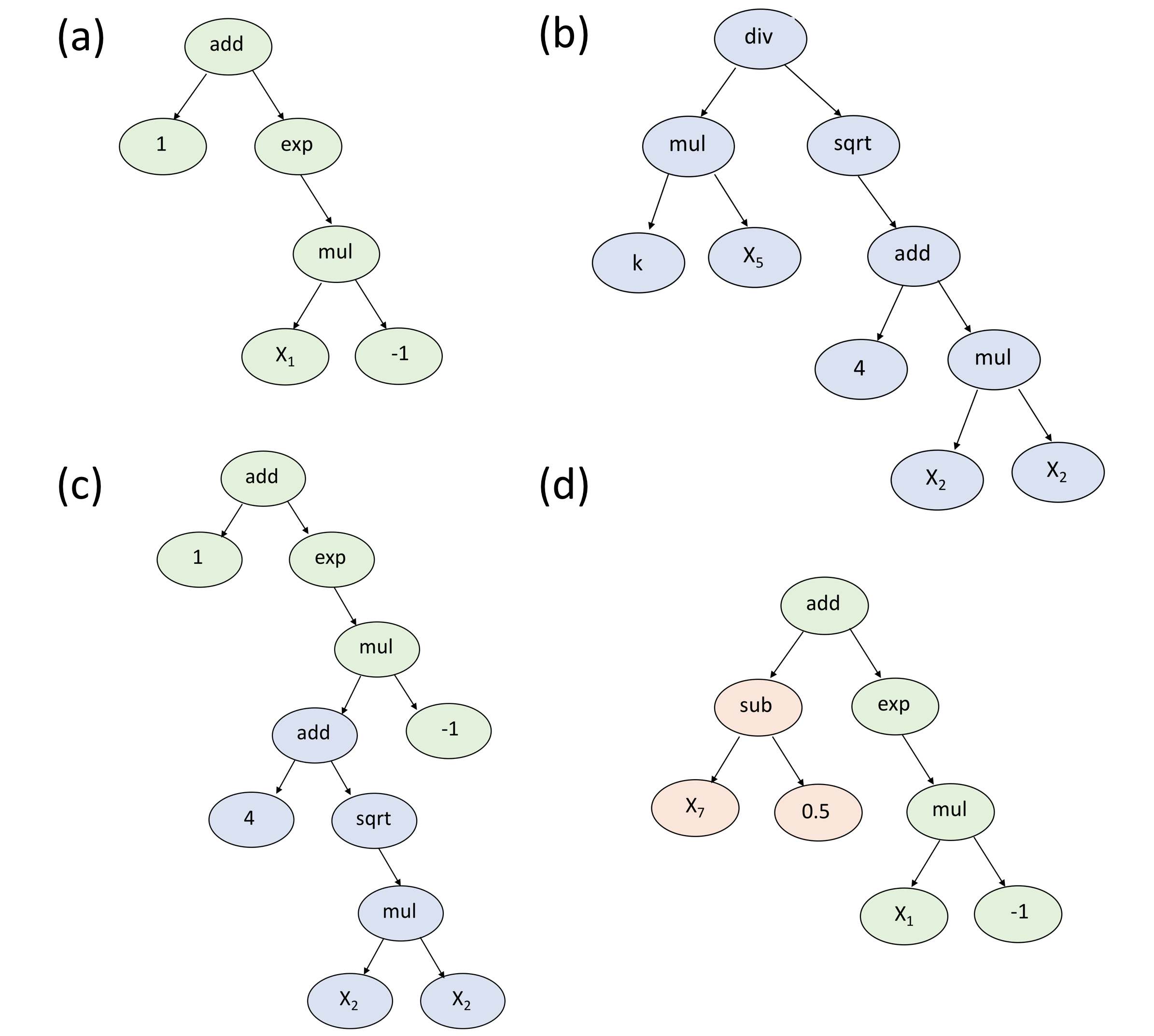
Genetic programming (GP) was developed by J.R. Koza Koza (1994) as a specific implementation of genetic algorithms (GA) Forrest (1993), which are often utilized in the materials community for atomic structure predictionMeredig and Wolverton (2013); Chua et al. (2010); Mohn et al. (2011). The idea is to evolve the solution of a given problem following Darwin’s theory of evolution and to find the fittest solution after a number of generations. Instead of using strings of binary digits to represent chromosomes as in GA, solutions in GP are represented as tree-structured chromosomes with nodes and terminals. Figure 2a shows a chromosome example of the mathematical function . The tree consists of a set of interior nodes with mathematical operations (, , ) and terminal nodes with variables () and constants (). A depth-first search can be used to traverse the tree to get the final mathematical expression of each individual solution.
The structure of a chromosome tree is not necessarily binary; its structure depends on the number of arguments the mathematical operator takes. For demonstration purposes, we only introduce simple operators that are either unary or binary. Users of GP could include a variety of functions suitable for their target problems. A large number of trees will be generated based on specified user settings and evaluated throughout the GP process. Each tree represents a potential solution of the problem. The way new trees are generated from the initial mathematical building blocks is a unique feature of GP since it mimics the natural evolution of Earth’s ecosystem, i.e. through artificial sexual recombination and a natural selection process.
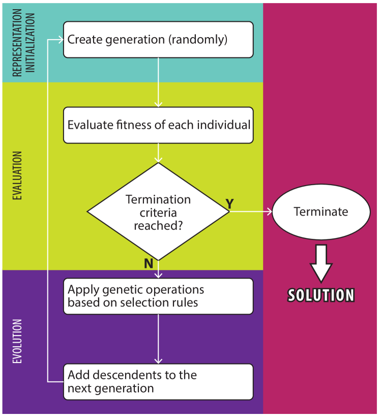
Figure 3 illustrates the process by which a solution of the symbolic regression problem is obtained using genetic programming. The procedure starts with a set of randomly generated initial terminal nodes (variables, constants) and functions, forming individual trees with different sizes and structures (Figure 2a-d). These fundamental building blocks come from a user-defined input set. This starting population typically has a large variety of tree structures due to the random process, which facilitates further exploration of the variable space and reduces the potential risk of being trapped in local minima. The initialization process terminates once the number of individuals reaches a user-defined population size, where the natural selection process then comes into play. The “fitness” of each individual solution in the initial population is then evaluated by comparing their function output with the true value from the data set. This fitness value describes how well the program performs in terms of solving the problem. The common error metrics used include mean squared error (MSE), root-mean squared error (RMSE), etc. Then GP evolves the current generation by randomly applying genetic operations to individuals, e.g. crossover and mutation. One or more individuals from the current generation will be selected as parent(s) based on the fitness score, typically the higher the score, the larger probability to be selected for reproduction. Such a selection rule agrees with the “survival-of-the-fittest” rule since good features are more likely to be inherited by the next generation, which is the essential step towards the optimal solution.
| Program representation | Fitness evaluation | Optimization | Solution form | |
| GPSR | rooted-tree | individual program | genetic evolution | rooted-tree |
| MRGP | rooted-tree | subexpressions | genetic evolution + | linear combination |
| linear regression | of subexpressions | |||
| GSGP | rooted-tree | distance in | genetic evolution in | rooted-tree/ |
| semantic space | semantic space | semantic vector | ||
| CGP | acyclic graph | individual program | genetic evolution | 2D grid of nodes |
| GP-RVM | rooted-tree | group of GP | genetic evolution + | linear combination of |
| individual | RVM | GP individuals | ||
| EPR | vector of integers | individual program | genetic evolution + | polynomial function |
| linear regression | ||||
| FFX | basis functions | individual program | pathwise regularized | linear combination of |
| learning | basis functions |
The genetic crossover operation takes two winners of the selection process as parents to breed their offspring. For instance, the two structures in Figure 2a and b are taken as parents. The crossover operator then randomly takes a subtree from parent (b) and substitutes another random subtree in parent (a) with that from (b). One possible offspring from the crossover operator is illustrated in Figure 2c. Crossover is usually the dominant operation in the recombination process. Figure 2d is an example of an offspring from the mutation operation. The mutation operator only takes one parent structure, and randomly substitutes a subtree with another randomly generated structure; in case (d), the constant 1 is mutated to . Although this operation is more aggressive compared to the crossover operation, since it adds randomness to the system, it is important to have a finite chance of mutation to introduce new variations, e.g. new constants and new features, and avoid being trapped in local minima.
The third category of genetic operations is reproduction, which duplicates the selected program and directly inserts its offspring to the next generation. It guarantees that some of the current generation will be preserved by the next generation, and partially protects the similarity between two generations. Detailed definitions and implementations of each genetic operation can vary from case to case, but the main features should be the similar to what we described here.
The newborns are then added to the next generation after each genetic operation, until the new population size reaches the specified set number. Then the new generation goes through the fitness evaluation and natural selection process again until the fitness value reaches a certain criteria or the maximum number of generations is reached. After termination of GP, the surviving individuals are expected to be highly evolved to adapt to the problem-dependent selection rule. More comprehensive descriptions of GP can be found in Koza’s original paperKoza (1994).
II.2 Advances in symbolic regression
Since Koza introduced the idea of GP in 1992, there have been significant efforts made to improve the performance of the original GPSR algorithm. The major problems to overcome in GPSR include:
-
()
Non-deterministic optimization. It is not guaranteed that the performance of the descendent generations will be better than their parents.
-
()
Difficulty in finding the proper constants. Since the way GP generates constants is random, either in the initial input set or those brought into the population by mutations, there is no effective way to obtain the ideal coefficients as in other numerical regression methods.
-
()
Limited capability to preserve good components of the equation due to the fitness evaluation method. The fitness is evaluated based on the complete structure of an individual. Having a good feature in a subbranch does not necessarily lead to better individual performance, thus good equation components may get lost in the next generation.
We summarize some of the most popular alternative methods to conventional GPSR in Table 1 and discuss their similarities as well as the differences in four aspects, namely program representation, fitness evaluation, optimization method, and the solution form.
Multiple regression genetic programming (MRGP) Arnaldo et al. (2014) improves the program evaluation process by performing multiple regression on subexpressions of the solution functions. Instead of evaluating the fitness of each individual solution as a whole, MRGP decouples its mathematical expression tree into subtrees. The fitness of the solution is evaluated based on the best linear combination of these subtree structures. A least angle regression (LARS) algorithm is used to solve the linear regression problem here. Such a fitness evaluation scheme places more emphasis on finding good components even though it might only be a partial solution. For instance, the individuals that contain a correct form of a subtree structure of the correct solution (if known) are more likely to survive the natural selection process and pass these good features to the descendents. MRGP essentially decouples the current basis functions to find the best solution in an enlarged space at the vicinity of the original GP space. Indeed, this feature may be well-suited for multi-scale materials problems where modeling of systems across different length/time-scale is desired Moore et al. (2014). While some subexpressions capture relationship among variables within each scale, the final symbolic regression solution assembles models across the scale and returns the multi-scale model.
Geometric semantic genetic programming (GSGP) Castelli et al. (2015) evaluates the semantic performance of a computer program instead of the syntax performance as in conventional GPSR. While still using a rooted-tree structure to represent computer programs, GSGP focuses on its semantics, i.e. the behavior of a program. For instance, is equivalent to in semantic space, but quite different in terms of syntax. It is reasonable to care more about the behavior of the program than how the function appears. By representing each program in a high-dimensional semantic space, the fitness evaluation is rather straightforward; one only needs to measure the distance of the program from the target point in that space. The closer a program is to the target point, the better performance it has in solving the given problem. Interestingly, the offspring of two parent vectors in semantic space lies between its parents in the semantic space; therefore, the offspring should be at least no worse performing than the poor-performing parent. Optimizing program semantics rather than syntax further frees symbolic regression from specific function forms, potentially making SR more efficient Castelli et al. (2015).
Cartesian genetic programming (CGP) Miller et al. (2000) has a more sophisticated design than conventional GP. Here, a computer program is represented as a directed acyclic graph, which may be visualized as a two-dimensional grid of nodes. Each node owns a set of genes that determines the input-output and mathematical function that the node performs; the whole set of genes of the computer programs form its genotype. Decoding the genotype leads to the phenotype, i.e. the function form of the computer programs. The genotype-phenotype mapping is a unique feature of CGP which makes it closer to the real natural process.
GP-RVM Rad et al. (2018) is an alternative GP method that combines Kaizen programming and a relevance vector machine (RVM) algorithm to solve symbolic regression problems. Kaizen programming (KP) is a collaborative version of genetic programming, where individuals work together with each other to solve the problem. The solution of a Kaizen process is a linear combination of GP individuals, and thus the fitness evaluation is based on a group of individual partial solutions instead of an individual program as a complete solution. RVM is a Bayesian kernel method that could extract important basis functions from the basis set without the prior knowledge to set a threshold and automatically deals with singularity. GP-RVM leverages advantages from both evolutionary algorithm and Bayesian kernel methods: the former mainly explores the parameter space while the latter extracts basis functions to build and solve for the optimal solution function within that space.
Evolutionary polynomial regression (EPR) Giustolisi and Savic (2009) hybridizes the parameter estimation used in conventional numerical regression methods with the evolutionary optimization scheme in GPSR. EPR first explores the function space using genetic algorithms, then performs linear regression (e.g. least squares) to optimize the coefficients of each mathematical building block. Although EPR specifically uses polynomial expansions for the form of the functions, the solution is not necessarily a simple polynomial function since the transformed variables used in the polynomial expansion could be nonlinear functions of independent input variables. Such a hybrid method improves the stochastic GPSR method moving it towards a more deterministic approach although the computational cost may be relatively higher. In fact, the polynomial form of the expressions could make EPR suitable for materials design or multiobjective optimization purposes. Since the analytical gradient and Hessian of the solution can be evaluated, materials scientists may have more insights regarding the system and know what parameters to tune in order to achieve optimal design.
Fast function extraction (FFX) McConaghy (2011) is an efficient way to find good basis functions and solve for the best solution within the space it spans. The first step in FFX is to generate a large number of candidate basis functions built from input variables and other predefined variables. The evolutionary optimization scheme is not involved in FFX, instead, a pathwise regularized learning technique is used to identify the best coefficients and basis functions for the solution. Then, models obtained from the previous step are assessed based on the validation data set as well as their model complexity in order to identify the best solution. FFX is more efficient compared to other GP-based methods due to the deterministic optimization technique. Materials scientists could first use FFX to see whether the input function/variable basis is sufficient for their research problem, before further investigation using symbolic regression methods (either FFX or other variants).
The performance of some of the recently developed symbolic regression techniques has been assessed against popular machine learning methods Orzechowski et al. (2018), and it is reported that symbolic regression performs considerably well compared to state of the art ML algorithms with regards to predictive accuracy. However, the two methods do not simply exist in competition to one another. We also observe a trend of more hybridization between conventional ML algorithms and genetic programming in symbolic regression solversIcke and Bongard (2013); Krawiec (2002); Lu et al. (2016); Li et al. (2019). These advances have enabled symbolic regression to be used for solving real-world problems, which we will discuss in the following section.
III Applications of symbolic regression
Although it seems that equations obtained from first principles (e.g., the Schrödiner equation) and empirical observations (e.g., the 18-electron rule Tolman (1972)) are quite contradictory to each other, we see quite often that they symbiotically work together in solving real-world problems. For instance, both ab initio and experimental data have been used to develop effective interatomic force fields Van Beest et al. (1990) or exchange-correlation functionalsYanai et al. (2004). In fact, symbolic regression has the potential to serve as the bridge connecting experimental data to first principles. Schmidt et al. demonstrated that symbolic regression is capable of predicting connections between dynamics of subcomponents of the system and distill natural laws from experimental data Schmidt and Lipson (2009a). Moreover, symbolic regression provides researchers with analytic equations, which expectably would have better interpretability over the raw data and potentially other black-box models. The equations could reveal how the dependent variable (system output) responds to multiple independent variables (system input), as well as the relationships between independent variables of the underlying function. We show this later in Section III.3.
Common motivations underlying the use of GPSR for complex problem solving include when the system in question is not effectively modelled by a linear model. Existing multiple linear regression models are much faster and are already easy to interpret. GPSR is best used for systems with complex interactions between observable variables for which the form of which is not known beforehand—a situation common in materials science and engineering.
In addition, a GPSR approach could be useful for design optimization purposes. Although the evolutionary search process is a black box, the final solution is analytical, which potentially contains important information (e.g., regarding the gradient or Hessian) about relationships between the design variables and objectives. There is also need for multi-objective optimization such as finding the Pareto optimal combination of model performance and complexity in various domains—it is here that the symbolic regression technique has shown to be effective and interpretable Gout et al. (2018). We next describe some applications of symbolic regression in various science and technology domains.
III.1 Industrial applications
GPSR has been applied to a wide variety of problems in fields outside of materials science and chemistry. Most prominently featured in the popular press was work published by Schmidt and Lipson in Science,Schmidt and Lipson (2009a) which showed GPSR could discover Hamiltonians and Lagrangians for systems of simple harmonic oscillators and double pendulums. Reports of using GPSR for real world systems, however, have been published since Koza’s origination of the idea in the early 1990s and continue today.
Arkov et al.Arkov et al. (2000) used GPSR to identify equations governing gas turbine engines under multiple optimization conditions. Berardi et al.Berardi et al. (2008) used GPSR to find easy to interpret models for pipe failures in a UK water distribution system. Bongard and LipsonBongard and Lipson (2007) applied GPSR to generate symbolic equations for nonlinear coupled dynamical systems in mechanics, ecology, and systems biology. The authors also emphasized that their symbolic models are easier to interpret than numerical models, which makes understanding more complex systems easier for future applications.
Cai et al.Cai et al. (2006) identified correlation equations from experimental heat transfer measurements using GPSR with a sparsifying constraint. The authors’ predicted correlations had lower percentage error than models developed graphically and numerically, albeit with more formula complexity than those traditional methods. Can and HeaveyCan and Heavey (2011) applied GPSR to develop metamodels for predicting throughput rates in industrial serial production lines. McKay, Willis and Barton developed steady-state models for a vacuum distillation column and a chemical reactorMcKay et al. (1997).
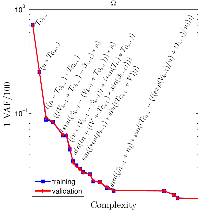
La Cava et al.La Cava et al. (2016a) applied GPSR to identify nonlinear governing equations of wind turbines. The Pareto front from their paper is reproduced in Figure 4. The Pareto front illustrates the trade-off between their model complexity as defined by the number and type of operations in the equation and the normalized variance in the prediction error. La Cava and other authorsLa Cava et al. (2016b) also tested modifying standard GPSR with features from epigenetics, such as passive structure, phenotypic plasticity, and inheritable gene regulation. These researchers demonstrated their modifications improved the performance over standard GPSR by finding compact dynamic equations for synthetic data from nonlinear ordinary differential equations as well as real-world systems, e.g. cascaded tanks, a chemical distillation tower, and an industrial wind turbine. GPSR has also been applied to testing the efficient market hypothesisChen and Yeh (1997), formulating the synchronization control in oscillator networksGout et al. (2018), identifying the structure of helicopter engine dynamicsGray et al. (1998), real-time runoff forecasting in FranceKhu et al. (2001) and SingaporeLiong et al. (2002), designing circuitsMiller et al. (2000), predicting solar power productionQuade et al. (2016), finding dynamical equations for metabolic networksSchmidt et al. (2011) in both cases where a starting model was known and from scratch, modelling global temperature changesStanislawska et al. (2012), and synthesizing second-order coefficient insensitive digital filter structuresUesaka and Kawamata (2000).
The existing uses of GPSR within chemistry are more extensive than that for materials science. We refer the reader to the review by Vyas, Goel, and TambeVyas et al. (2015) for further details. Some key studies with relevance to materials science are summarized here: Langdon and Barrett developed a model for oral bioavailability of a small molecule given a few hundred data points from expensive experimentsLangdon and Barrett (2005). Their model based on chemical descriptors showed promise for rapid drug screening, but had difficulty generalizing to novel molecules. Vyas et al.Vyas et al. (2014) also discovered structure-property relationships for drug absorption using GPSR. Here, they demonstrated values comparable to those achieved with artificial neural networks and support vector regression. Barmpalexis et al.Barmpalexis et al. (2011) performed a multiobjective optimization using GPSR. They found a function mapping levels of 4 polymers to three different properties of a pharmaceutical release tablet that was more predictive than a shallow neural network. Last, Muzny, Huber, and Kazakov built a correlation model for the viscosity of hydrogen as a function of temperature and pressureMuzny et al. (2013).
III.2 Opportunities in materials science
Materials science has many potential areas where GPSR can be applied for the same reasons it find use in other disciplines. Nonlinear systems are abundant in materials science. Changes in materials properties occuring in response to structural, composition, and other external perturbations are frequently nonlinear in proximity to phase transitions or for large stimuli. For instance, changing the concentration of oxygen vacancies in a transition metal compound by an atomic percent can alter its ionic or electronic conductivity by orders of magnitudeMarkov et al. (2007); Nakamura and Wagner . The dynamical behavior of materials performance as a function of time is also of broad interest and technological importance, e.g. corrosion of nickel cathodes under different conditions Daza et al. (2000). These are the areas where a dynamical multivariable model would be ideal to understand the correlation among the variables and assist optimization of materials properties, e.g. corrosion resistance.
Frequently, materials scientists look for relationships () among multiple variables with the aim to find some closed-form expression such as , where is the objective value and are a set of variables. These equations are typically expressed in differential form, e.g., the Schrödinger equation () or Newton’s second law (). It has been shown that symbolic regression can generate ordinary nonlinear partial differential equations for nonlinear coupled dynamical systems Bongard and Lipson (2007); Maslyaev et al. (2019) as well as approximate ordinary differential equationsGaucel et al. (2014). Meanwhile, it is also often of desire to find conservation laws in physical systems. The ability to unearth conservation laws with symbolic regression goes beyond the aim of materials property predictions and helps researchers establish insight into the materials systems they studySchmidt and Lipson (2009a, b). In fact, we do not necessarily need a rigorous expression of natural laws in every case; sometimes an approximation with a simple yet effective expression serves well for the research purposevon Barth and Hedin (1972). Symbolic regression could potentially balance the trade-off between model accuracy and simplicity, and might even help scientists discover new equations that redefine our understanding of functional materials in the same way those of Hall and Petch and Harper and Dorn changed our understanding of the mechanical properties of metals or as more recently how Berry phases and topological band theory changed our understanding of electronic structures.
As we mentioned earlier, materials properties and performance are affected by phenomena that involve multiple length scales. Most theoretical models are formulated to be optimal at a particular length scale. However, recent emphasis has been placed on multiscale and hiearchical modeling in the materials science community mul (2015); Yadollahi et al. (2015); Moore et al. (2014), and there is an increased need for effective, descriptive and predicative, multiscale models. Symbolic regression techniques are potential solutions to this challenge by directly searching for the interactions among variables operating and passing between multiple spatial and temporal scales. Another possible approach is to utilize existing simulation methods within each length scale, while using symbolic regression to find the suitable coupling interactions between scales, i.e. connecting models of different scales.
Other applications of GPSR in materials and molecular systems are in areas where supervised machine learning has already demonstrated usefulness in providing new insight or solutions. While machine learning has produced many impressive resultsZhuo et al. (2018); Alberi et al. (2019); Ward and Wolverton (2017), it is commonly understood that ML models exhibit a trade-off between performance on prediction metrics and the ability to explain the predictions of a model due to the complexity of state-of-the-art models like deep neural networks or gradient boosted decision trees. GPSR offers a middle ground with comparable performance but with the added ability to read and directly interpret the output function.
GPSR is also well-suited to the development of new descriptorsGhiringhelli et al. (2015) for materials properties. By combining features in a manner best suited to fitting data, new features are created that can be used as proxies for the property in question. This is also a common application of compressed sensing Ghiringhelli et al. (2017); Ouyang et al. (2018). Compressed sensing differs from GPSR in that while GPSR uses GP to iteratively evolve a solution, compressed sensing tries to enumerate as many combinations of primary features as possible and then use sparsifying operators to find a small dimensional subset that correlates with the target.
Materials scientists are not just interested in making predictions. They also want to identify the controlling features of a property and what role each feature plays; they want to understand which degrees-of-freedom to design or optimize to achieve targeted properties. Given some desired properties as objectives and the relevant variables, there are a number of numerical algorithms available for performing optimization Vanderplaats (2001), but they typically require some a-priori knowledge of the mathematical relationships within the system. The symbolic equations derived from GPSR offer insight into which microscopic or macroscopic knobs to turn for the design of desired functionality, such as corrosion resistance in steelsShimada et al. (2002).
Some novel ideas include targeting physical variables for which we do not know the proper mathematical expressions. For instance, the exchange-correlation functional used in density functional theory, or the correlation function for the viscosity of normal hydrogen Muzny et al. (2013). Contraindicated material property pairs such as ferromagnetism and ferroelectricity or optical transparency and electrical conductivity would be interesting areas to pursue in search for routes to decouple or circumvent perceived coexistence incompatibilities. In these cases, GPSR could provide candidate representations of these terms, where our physical knowledge can be used to filter meaningful results. One advantage of using symbolic regression is that the balance between model accuracy and complexity is tunable with GPSR settings, e.g. stopping criteria, penalty on individual size, etc. This advantage is particularly evident when designing with constraints or optimizing for performance. The recommendations coming from the learned symbolic equations are more actionable than learned functions only optimized for test set accuracy since they are rigorously made to use fewer terms.
III.3 Use cases in materials science
III.3.1 Discovering the Johnson-Mehl-Avrami-
Kolmogorov equation
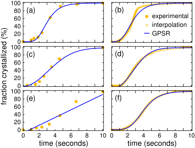
We now show how to use genetic programming-based symbolic regression to learn the Johnson-Mehl-Avrami-Kolmogorov (JMAK), hereafter, Avrami equation. The Avrami equation quantitatively describes the growth kinetics of phases in materials at constant temperature. Here, we specifically study the recrystallization process of copper, the original experimental data was obtained from Ref. Decker and Harker, 1950. We expect the form of the function to be
where the phase fraction of transformation is a function of time . The coefficients and are unknown and change with respect to temperature and other environmental conditions.
We use GPSR as implemented in gplearn Stephens (2016) to predict the relationship between fraction transformed and time . The hyper-parameters used in GPSR are listed in Table 2. When the population size is divided by the tournament factor, one obtains the number of individuals competing for reproduction each round. The parsimony coefficient regularizes the size of individuals by penalizing over-sized structures. We include operations of addition, subtraction, multiplication, negation, and the natural exponential function into the function set. The power function is not included since it easily causes numerical overflow or invalid operations (e.g. power(-1,0.5)). In general, this can be an issue when evaluating power-law dependent phenomena such as electrical transport equations. Working with log transforms of the original variables may be a more stable approach. Crossover operations dominate the genetic operations with a 70% probability to be applied; the other 30% chance corresponds to mutation operations (e.g. point mutation, subtree mutation, etc.). Additional details concerning the usage of gplearn are given in its documentation.
| Parameter | Values |
|---|---|
| population size | {2000, 5000} |
| tournament factor | {100, 500} |
| parsimony coefficient | {0.001, 0.005} |
| max generation | 20 |
| constant range | (-1, 1) |
| function set | {add, sub, mul, neg, exp} |
| crossover probability | 0.7 |
Data preprocessing is an essential step in machine learning before feeding data into the solver. Conventional preprocessing methods include shifting data to be zero-centered, and scaling data to unit standard deviation. However, the conventional preprocessing methods are not ideal choices in our case. Zero-centered shifting is not applicable to either the phase fraction transformed () or time () since we want to obtain the exact function form of the Avrami equation. Furthermore, scaling the time frame would only change the constant in the Avrami equation. Here, we scale time from 0 to 10 for all data sets so that the constant lies in the range [-1, 1]. The values remain unchanged as the experimental data range over [0, 1].
| Dataset | Numerical fitting result | GPSR result | GPSR (transformed ) result |
|---|---|---|---|
| ideal | |||
| 135∘C experimental | |||
| 135∘C interpolated | |||
| 113∘C experimental | |||
| 113∘C interpolated | |||
| 102∘C experimental | |||
| 102∘C interpolated |
We take the experimental copper recrystallization data at temperatures 135∘C, 113∘C, and 102∘C as input and scale the time variable before performing regression. Since the experimental data only contains several points at each temperature (less than 10), we also take data points from interpolated lines and perform symbolic regression on the interpolated data for comparison. An ideal dataset is also generated, where values are directly calculated as . The optimal and values in each data set are obtained from numerical fitting using Scipy, given the form of the Avrami function. Ideally GPSR should be able to recover the correct function form as well as and constants for all data sets.
The best individual after 20 generations of evolution is collected for each hyper-parameter setting. Finally we manually pick the optimal individual with closest function form and constants to the Avrami equation within each data set. Our parameter fitting and GPSR evolution results are shown in Table 3 and Figure 5.
Gplearn successfully recovers the relationship between time () and fraction transformed () in most cases. With the ideal input data, gplearn evolves almost a perfect form of the Avarmi function as well as the constants (see the first row of Table 3). The performance on the raw experimental and interpolated data are generally worse than the ideal case but still reasonable. In most cases the exponential function form and polynomial function of are both recovered. One source of error is the lack of the power function in function set, which was intentionally omitted as non-integer powers of variables cannot be correctly represented here. Rather, polynomial functions are used as an approximation. With the limited choice of mathematical functions, GP produces results that are very close semantically but exhibit different syntax.
We see in multiple cases GPSR produces functions of the form, where the expected function form is . Here we introduce a mathematical trick to show their equivalence. The functions and are called equivalent infinitesimals because
In our case, the exponent quickly reaches zero when (ideally having the form ) becomes more negative; therefore, the equivalent infinitesimal relationship holds and the predicted form of the function is equivalent to the expected one appearing in the Avrami expression. Based on this example, we encourage professional materials researchers, who are novice data scientists, to perform careful analysis of GPSR results when making the final interpretation of the obtained model.
In real-world applications where the actual function form in unknown, the exact syntax of GPSR results may not matter. There are potentially many cases where GPSR would produce semantically similar/equivalent functions that vary in their syntax, i.e. different function form. Considering the trade-off between model accuracy and complexity, in some cases it might be a virtue to find a simple approximated solution instead of using rigorous but complex relationships among multiple variables.
The GPSR result from the 102∘C experimental data set (Figure 5e), turns out to be a linear relationship and deviates significantly from the original data. The poor result may be caused by the relatively small slope of the original data and the insufficient number of available data points. Taking the model performance and complexity into consideration, we find that the linear relationship survives due to its simple form. With interpolated data as input, functions evolved from GPSR agree better with the Avrami equation, as shown in Figure 5f. Therefore, having more training data could improve the performance of GPSR, which also applies to other data-driven methods.
Interestingly, the performance of GPSR can also be improved by transforming (or simplifying) the mathematical expression. We compare results of directly training relationships with , where in the latter case the target value is the percentage of copper untransformed. The results are shown in the last column of Table 3: The transformed functions show improved performance since we have already performed the subtraction function for the model. GPSR not only successfully recovers the exponential form of the equation, but also finds constants closer to the numerical fitting values.
III.3.2 Learning Landau free energy expansion
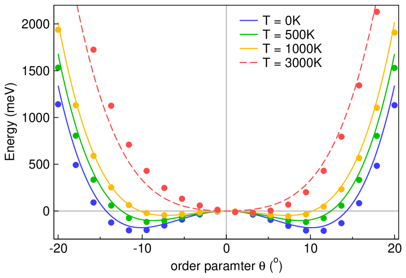
Next, we present a slightly more complicated case with two variables. The model we studied is the Landau free energy expansion for the cubic-to-rhombohedral structural phase transition in perovskite LaNiO3, where the free energy of the system is expanded in powers of an order parameter as
| (1) |
where and are temperature-independent coefficients and is the angle of rotation about the [111] direction. This rotation angle of the corner-connected NiO6 is the order parameter for the displacive transition. The parameters we used are obtained from ab initio DFT simulationsGou et al. (2011), where , , and is estimated to be . We use as the unit for temperature so that the constants are brought into a smaller range.
In this case, we set the temperature and order parameter as the input variables, and the free energy change as the output. We uniformly sampled 11 temperature points between [0, 1] (), and 100 order parameter points within range [-20∘, 20∘]. The corresponding value for the change in free energy is calculated from Equation 1 using the parameters reported in the literature. A population size of 10,000 is used, with tournament size 25, parsimony coefficient 0.02, and constant range [-2.0, 2.0]. In order to simplify the problem, we only consider addition, subtraction, and multiplication operations in our search. Other settings are the same to those in the Avrami case.
The best individual after 15 generations of evolution has the function form
| (2) |
where , and . The GPSR-learned coefficients are quite close to the reported values, especially for the quartic term. This is probably because the penalty for a larger deviation in the leading (quartic) term is much higher than others. For the quadratic term of , GPSR successfully captured the coupling term and its coefficient, but also an unexpected biquadratic . It should not have a strong impact on the function owing to its small coefficient ().
The Landau free energy with respect to the order parameter is plotted in Figure 6. We find that GPSR results (filled symbols) agree well with the DFT-derived Landau free energy function not only within the training region, i.e., with and , but also reasonably well beyond it. The dashed red line in Figure 6 with is not included in training the GPSR, yet the model reproduces both the shape and the correct global minimum position very well. However, the predicted function contains other coupling terms not present in Equation 1. These extra terms in destroy the symmetry of the function, i.e., the free energy expansion is an even function by symmetry. This would become an issue especially when is large, as we can see a minor shift to positive values occurs for the red filled symbols in Figure 6. Again, the model may need more data to learn the correct even function form. In general, GPSR does an excellent job in learning the relationship between temperature and the order parameter without any knowledge of the physical system. Our results here also reveal the potential to perform effective feature selection using GPSR, where the insignificant variables (features) could be approximated or ignored in post-processing (e.g. terms with negligibly small coefficients).
The purpose of these two use cases for learning the Avrami equation and Landau free energy expansion with GPSR is to show the potential of its application in materials science problems. Although these are relatively simple examples, the understanding and approaches applied could be generalized and utilized to solve real-world challenges. Apart from both function analysis and data pre-processing mentioned previously, hyper-parameter tuning is also an essential step to obtain the optimal solution. A grid-search scheme to search the hyper-parameter space (e.g., population size, number of generations, regularization, etc.) is recommended since the optimal settings differ from case to case. The grid-searching process can be exhausting, but it might also be rewarding. Comparing the results from different hyper-parameter settings could provide insight into the functional form of the optimal solution, especially if components of a particular function appears multiple times in the solution set.
The real challenge, however, is that very often materials science problems cannot be represented using regular functions (analytic and single-valued). A simple example would be to understand how different chemical compositions affect materials propertiesYu et al. (2016). This problem originates from the inability to differentiate in the chemical space and is out of the scope of this prospective. It remains an open question in the materials research community.
IV Summary
Symbolic regression has shown competitive performance to other machine learning-based regression models in various research domains. While there are some shortcomings of the current state-of-the-art GPSR, e.g. high computational cost, non-deterministic optimization, there are numerous active research efforts focusing on improving the performance of symbolic regression to expand its use in real-world applications. The ability of symbolic regression to distill natural laws from data sets with high-dimensional parameter space makes it an ideal technique for materials science research, since these researchers typically face sparse data sets with multiple variables. Freed from having a fixed form of equations, symbolic regression can potentially reveal the significant interactions among physical variables. We recommend more materials scientists utilize symbolic regression techniques in their own research domain.
Acknowledgements.
Y.W. acknowledges partial support from the Predictive Science and Engineering Design (PS&ED) program at Northwestern University. All authors acknowledge support from the National Science Foundation (NSF) through the Designing Materials to Revolutionize and Engineer our Future (DMREF) program under award number DMR-1729303.References
- Deelman et al. (2017) Ewa Deelman, Christopher Carothers, Anirban Mandal, Brian Tierney, Jeffrey S. Vetter, Ilya Baldin, Claris Castillo, Gideon Juve, Dariusz Król, Vickie Lynch, Ben Mayer, Jeremy Meredith, Thomas Proffen, Paul Ruth, and Rafael Ferreira da Silva, “PANORAMA: An approach to performance modeling and diagnosis of extreme-scale workflows,” The International Journal of High Performance Computing Applications 31, 4–18 (2017).
- Lupini et al. (2018) Andrew R. Lupini, Mark P. Oxley, and Sergei V. Kalinin, “Pushing the limits of electron ptychography,” Science 362, 399–400 (2018).
- Ren et al. (2017) Fang Ren, Ronald Pandolfi, Douglas Van Campen, Alexander Hexemer, and Apurva Mehta, “On-the-Fly Data Assessment for High-Throughput X-ray Diffraction Measurements,” ACS Combinatorial Science 19, 377–385 (2017).
- Stein et al. (2019) Helge S. Stein, Dan Guevarra, Paul F. Newhouse, Edwin Soedarmadji, and John M. Gregoire, “Machine learning of optical properties of materials – predicting spectra from images and images from spectra,” Chemical Science 10, 47–55 (2019).
- Alberi et al. (2019) Kirstin Alberi, Marco Buongiorno Nardelli, Andriy Zakutayev, Lubos Mitas, Stefano Curtarolo, Anubhav Jain, Marco Fornari, Nicola Marzari, Ichiro Takeuchi, Martin L Green, Mercouri Kanatzidis, Mike F Toney, Sergiy Butenko, Bryce Meredig, Stephan Lany, Ursula Kattner, Albert Davydov, Eric S Toberer, Vladan Stevanovic, Aron Walsh, Nam-Gyu Park, Alán Aspuru-Guzik, Daniel P Tabor, Jenny Nelson, James Murphy, Anant Setlur, John Gregoire, Hong Li, Ruijuan Xiao, Alfred Ludwig, Lane W Martin, Andrew M Rappe, Su-Huai Wei, and John Perkins, “The 2019 materials by design roadmap,” Journal of Physics D: Applied Physics 52, 013001 (2019).
- Green et al. (2017) M. L. Green, C. L. Choi, J. R. Hattrick-Simpers, A. M. Joshi, I. Takeuchi, S. C. Barron, E. Campo, T. Chiang, S. Empedocles, J. M. Gregoire, A. G. Kusne, J. Martin, A. Mehta, K. Persson, Z. Trautt, J. Van Duren, and A. Zakutayev, “Fulfilling the promise of the materials genome initiative with high-throughput experimental methodologies,” Applied Physics Reviews 4, 011105 (2017), https://doi.org/10.1063/1.4977487 .
- Ye et al. (2018) Weike Ye, Chi Chen, Shyam Dwaraknath, Anubhav Jain, Shyue Ping Ong, and Kristin A. Persson, “Harnessing the Materials Project for machine-learning and accelerated discovery,” MRS Bulletin 43, 664–669 (2018).
- Tanaka et al. (2018) Isao Tanaka, Krishna Rajan, and Christopher Wolverton, “Data-centric science for materials innovation,” MRS Bulletin 43, 659–663 (2018).
- Kim et al. (2017) Edward Kim, Kevin Huang, Adam Saunders, Andrew McCallum, Gerbrand Ceder, and Elsa Olivetti, “Materials Synthesis Insights from Scientific Literature via Text Extraction and Machine Learning,” Chemistry of Materials 29, 9436–9444 (2017).
- Krallinger et al. (2017) Martin Krallinger, Obdulia Rabal, Anália Lourenço, Julen Oyarzabal, and Alfonso Valencia, “Information retrieval and text mining technologies for chemistry,” (2017).
- Government (2014) U.S. Government, “Materials Genome Initiative National Science and Technology Council Committee on Technology Subcommittee on the Materials Genome Initiative JUNE 2014,” Whitehouse.Gov (2014).
- Jain et al. (2013) Anubhav Jain, Shyue Ping Ong, Geoffroy Hautier, Wei Chen, William Davidson Richards, Stephen Dacek, Shreyas Cholia, Dan Gunter, David Skinner, Gerbrand Ceder, and Kristin A. Persson, “Commentary: The Materials Project: A materials genome approach to accelerating materials innovation,” APL Materials 1, 011002 (2013).
- Saal et al. (2013) James E. Saal, Scott Kirklin, Muratahan Aykol, Bryce Meredig, and C. Wolverton, “Materials design and discovery with high-throughput density functional theory: The open quantum materials database (OQMD),” Jom 65, 1501–1509 (2013).
- Curtarolo et al. (2012) Stefano Curtarolo, Wahyu Setyawan, Shidong Wang, Junkai Xue, Kesong Yang, Richard H. Taylor, Lance J. Nelson, Gus L.W. Hart, Stefano Sanvito, Marco Buongiorno-Nardelli, Natalio Mingo, and Ohad Levy, “AFLOWLIB.ORG: A distributed materials properties repository from high-throughput ab initio calculations,” Computational Materials Science 58, 227–235 (2012).
- Borysov et al. (2017) Stanislav S. Borysov, R. Matthias Geilhufe, and Alexander V. Balatsky, “Organic materials database: An open-access online database for data mining,” PLOS ONE 12, e0171501 (2017).
- Pizzi et al. (2016) Giovanni Pizzi, Andrea Cepellotti, Riccardo Sabatini, Nicola Marzari, and Boris Kozinsky, “AiiDA: automated interactive infrastructure and database for computational science,” Computational Materials Science 111, 218–230 (2016), arXiv:1504.01163v1 .
- Zhuo et al. (2018) Ya Zhuo, Aria Mansouri Tehrani, Anton O. Oliynyk, Anna C. Duke, and Jakoah Brgoch, “Identifying an efficient, thermally robust inorganic phosphor host via machine learning,” Nature Communications 9, 4377 (2018).
- Hall and Gill (2018) Patrick Hall and Navdeep Gill, An Introduction to Machine Learning Interpretability, 1st ed. (2018).
- (19) “webofscience,” .
- Augusto and Barbosa (2000) D. A. Augusto and H. J.C. Barbosa, “Symbolic regression via genetic programming,” in Proceedings - Brazilian Symposium on Neural Networks, SBRN, Vol. 2000-Janua (IEEE Comput. Soc, 2000) pp. 173–178.
- Seber and Lee (2003) G. A. F. (George Arthur Frederick) Seber and A. J. Lee, Linear regression analysis (Wiley-Interscience, 2003) p. 557.
- Koza (1994) John R. Koza, “Genetic programming as a means for programming computers by natural selection,” Statistics and Computing 4, 87–112 (1994).
- Forrest (1993) Stephanie Forrest, “Genetic algorithms: principles of natural selection applied to computation,” Science 261, 872–878 (1993).
- Meredig and Wolverton (2013) Bryce Meredig and C. Wolverton, “A hybrid computational–experimental approach for automated crystal structure solution,” Nature Materials 12, 123–127 (2013).
- Chua et al. (2010) Alvin L.-S. Chua, Nicole A. Benedek, Lin Chen, Mike W. Finnis, and Adrian P. Sutton, “A genetic algorithm for predicting the structures of interfaces in multicomponent systems,” Nature Materials 9, 418–422 (2010).
- Mohn et al. (2011) Chris E. Mohn, Svein Stølen, and Walter Kob, “Predicting the Structure of Alloys Using Genetic Algorithms,” Materials and Manufacturing Processes 26, 348–353 (2011).
- Arnaldo et al. (2014) Ignacio Arnaldo, Krzysztof Krawiec, and Una-May O’Reilly, “Multiple regression genetic programming,” in Proceedings of the 2014 conference on Genetic and evolutionary computation - GECCO ’14 (ACM Press, New York, New York, USA, 2014) pp. 879–886.
- Moore et al. (2014) John A. Moore, Ruizhe Ma, August G. Domel, and Wing Kam Liu, “An efficient multiscale model of damping properties for filled elastomers with complex microstructures,” Composites Part B: Engineering 62, 262–270 (2014).
- Castelli et al. (2015) Mauro Castelli, Sara Silva, and Leonardo Vanneschi, “A C++ framework for geometric semantic genetic programming,” (2015).
- Miller et al. (2000) Julian F. Miller, Dominic Job, and Vesselin K. Vassilev, “Principles in the Evolutionary Design of Digital Circuits—Part I,” Genetic Programming and Evolvable Machines 1, 7–35 (2000).
- Rad et al. (2018) Hossein Izadi Rad, Ji Feng, and Hitoshi Iba, “GP-RVM: Genetic Programing-based Symbolic Regression Using Relevance Vector Machine,” (2018), arXiv:1806.02502v2, arXiv:1806.02502 .
- Giustolisi and Savic (2009) O. Giustolisi and D. A. Savic, “Advances in data-driven analyses and modelling using EPR-MOGA,” Journal of Hydroinformatics 11, 225 (2009).
- McConaghy (2011) Trent McConaghy, “FFX: Fast, Scalable, Deterministic Symbolic Regression Technology,” (Springer, New York, NY, 2011) pp. 235–260.
- Orzechowski et al. (2018) Patryk Orzechowski, William La Cava, and Jason H. Moore, “Where are we now?” in Proceedings of the Genetic and Evolutionary Computation Conference on - GECCO ’18 (ACM Press, New York, New York, USA, 2018) pp. 1183–1190, arXiv:1804.09331 .
- Icke and Bongard (2013) Ilknur Icke and Joshua C. Bongard, “Improving genetic programming based symbolic regression using deterministic machine learning,” in 2013 IEEE Congress on Evolutionary Computation (IEEE, 2013) pp. 1763–1770.
- Krawiec (2002) Krzysztof Krawiec, “Genetic programming-based construction of features for machine learning and knowledge discovery tasks,” Genetic Programming and Evolvable Machines 3, 329–343 (2002).
- Lu et al. (2016) Qiang Lu, Jun Ren, and Zhiguang Wang, “Using genetic programming with prior formula knowledge to solve symbolic regression problem,” Computational intelligence and neuroscience 2016, 1 (2016).
- Li et al. (2019) Li Li, Minjie Fan, Rishabh Singh, and Patrick Riley, “Neural-guided symbolic regression with semantic prior,” arXiv preprint arXiv:1901.07714 (2019).
- Tolman (1972) CA Tolman, “The 16 and 18 electron rule in organometallic chemistry and homogeneous catalysis,” Chemical Society Reviews 1, 337–353 (1972).
- Van Beest et al. (1990) BWH Van Beest, Gert Jan Kramer, and RA Van Santen, “Force fields for silicas and aluminophosphates based on ab initio calculations,” Physical Review Letters 64, 1955 (1990).
- Yanai et al. (2004) Takeshi Yanai, David P Tew, and Nicholas C Handy, “A new hybrid exchange–correlation functional using the coulomb-attenuating method (cam-b3lyp),” Chemical Physics Letters 393, 51–57 (2004).
- Schmidt and Lipson (2009a) Michael Schmidt and Hod Lipson, “Distilling free-form natural laws from experimental data,” Science 324, 81–85 (2009a).
- Gout et al. (2018) Julien Gout, Markus Quade, Kamran Shafi, Robert K. Niven, and Markus Abel, “Synchronization control of oscillator networks using symbolic regression,” Nonlinear Dynamics 91, 1001–1021 (2018).
- Arkov et al. (2000) V. Arkov, C. Evans, P. J. Fleming, D. C. Hill, J. P. Norton, I. Pratt, D. Rees, and K. Rodríguez-Vázquez, “System identification strategies applied to aircraft gas turbine engines,” Annual Reviews in Control 24, 67–81 (2000).
- Berardi et al. (2008) L. Berardi, O. Giustolisi, Z. Kapelan, and D. A. Savic, “Development of pipe deterioration models for water distribution systems using EPR,” Journal of Hydroinformatics 10, 113 (2008), arXiv:1406.6111 .
- Bongard and Lipson (2007) J. Bongard and H. Lipson, “Automated reverse engineering of nonlinear dynamical systems,” Proceedings of the National Academy of Sciences 104, 9943–9948 (2007).
- Cai et al. (2006) Weihua Cai, Arturo Pacheco-Vega, Mihir Sen, and K. T. Yang, “Heat transfer correlations by symbolic regression,” International Journal of Heat and Mass Transfer 49, 4352–4359 (2006).
- Can and Heavey (2011) Birkan Can and Cathal Heavey, “Comparison of experimental designs for simulation-based symbolic regression of manufacturing systems,” Computers and Industrial Engineering 61, 447–462 (2011).
- McKay et al. (1997) Ben McKay, Mark Willis, and Geoffrey Barton, “Steady-state modelling of chemical process systems using genetic programming,” Computers and Chemical Engineering 21, 981–996 (1997).
- La Cava et al. (2016a) William La Cava, Kourosh Danai, and Lee Spector, “Inference of compact nonlinear dynamic models by epigenetic local search,” Engineering Applications of Artificial Intelligence 55, 292–306 (2016a).
- La Cava et al. (2016b) William La Cava, Kourosh Danai, Lee Spector, Paul Fleming, Alan Wright, and Matthew Lackner, “Automatic identification of wind turbine models using evolutionary multiobjective optimization,” Renewable Energy 87, 892–902 (2016b).
- Chen and Yeh (1997) Shu-Heng Chen and Chia-Hsuan Yeh, “Toward a computable approach to the efficient market hypothesis: An application of genetic programming,” Journal of Economic Dynamics and Control 21, 1043–1063 (1997).
- Gray et al. (1998) Gary J. Gray, David J. Murray-Smith, Yun Li, Ken C. Sharman, and Thomas Weinbrenner, “Nonlinear model structure identification using genetic programming,” Control Engineering Practice 6, 1341–1352 (1998).
- Khu et al. (2001) Soon Thiam Khu, Shie Yui Liong, Vladan Babovic, Henrik Madsen, and Nitin Muttil, “Genetic programming and its application in real-time runoff forecasting,” Journal of the American Water Resources Association 37, 439–451 (2001).
- Liong et al. (2002) Shie-Yui Liong, Tirtha Raj Gautam, Soon Thiam Khu, Vladan Babovic, Maarten Keijzer, and Nitin Muttil, “GENETIC PROGRAMMING: A NEW PARADIGM IN RAINFALL RUNOFF MODELING,” Journal of the American Water Resources Association 38, 705–718 (2002).
- Quade et al. (2016) Markus Quade, Markus Abel, Kamran Shafi, Robert K. Niven, and Bernd R. Noack, “Prediction of dynamical systems by symbolic regression,” Physical Review E 94, 012214 (2016), arXiv:1602.04648 .
- Schmidt et al. (2011) Michael D. Schmidt, Ravishankar R. Vallabhajosyula, Jerry W. Jenkins, Jonathan E. Hood, Abhishek S. Soni, John P. Wikswo, and Hod Lipson, “Automated refinement and inference of analytical models for metabolic networks,” Physical Biology 8, 055011 (2011).
- Stanislawska et al. (2012) Karolina Stanislawska, Krzysztof Krawiec, and Zbigniew W. Kundzewicz, “Modeling global temperature changes with genetic programming,” Computers & Mathematics with Applications 64, 3717–3728 (2012).
- Uesaka and Kawamata (2000) Kazuyoshi Uesaka and Masayuki Kawamata, “Synthesis of low-sensitivity second-order digital filters using genetic programming with automatically defined functions,” IEEE Signal Processing Letters 7, 83–85 (2000).
- Vyas et al. (2015) Renu Vyas, Purva Goel, and Sanjeev S. Tambe, “Genetic programming applications in chemical sciences and engineering,” in Handbook of Genetic Programming Applications (Springer International Publishing, Cham, 2015) pp. 99–140.
- Langdon and Barrett (2005) W B Langdon and S J Barrett, “Genetic Programming in Data Mining for Drug Discovery,” in Evolutionary Computation in Data Mining, Vol. 163 (Springer-Verlag, Berlin/Heidelberg, 2005) pp. 211–235.
- Vyas et al. (2014) Renu Vyas, Purva Goel, M. Karthikeyan, S.S. Tambe, and B.D. Kulkarni, “Pharmacokinetic Modeling of Caco-2 Cell Permeability Using Genetic Programming (GP) Method,” Letters in Drug Design & Discovery 11, 1112–1118 (2014).
- Barmpalexis et al. (2011) P. Barmpalexis, K. Kachrimanis, A. Tsakonas, and E. Georgarakis, “Symbolic regression via genetic programming in the optimization of a controlled release pharmaceutical formulation,” Chemometrics and Intelligent Laboratory Systems 107, 75–82 (2011).
- Muzny et al. (2013) Chris D. Muzny, Marcia L. Huber, and Andrei F. Kazakov, “Correlation for the Viscosity of Normal Hydrogen Obtained from Symbolic Regression,” Journal of Chemical & Engineering Data 58, 969–979 (2013).
- Markov et al. (2007) Alexey A Markov, Mikhail V Patrakeev, Vladislav V Kharton, Yevheniy V Pivak, Ilia A Leonidov, and Viktor L Kozhevnikov, “Oxygen Nonstoichiometry and Ionic Conductivity of Sr 3 Fe 2 - x Sc x O 7 - ,” Chemistry of Materials 19, 3980–3987 (2007).
- (66) Akio Nakamura and J Bruce Wagner, Defect Structure, Ionic Conductivity, and Diffusion in Yttria Stabilized Zirconia and Related Oxide Electrolytes with Fluorite Structure, Tech. Rep.
- Daza et al. (2000) L Daza, C M Rangel, J Baranda, M T Casais, M. J. Martínez, and J A Alonso, “Modified nickel oxides as cathode materials for MCFC,” Journal of Power Sources 86, 329–333 (2000).
- Maslyaev et al. (2019) Michail Maslyaev, Alexander Hvatov, and Anna Kalyuzhnaya, “Data-driven PDE discovery with evolutionary approach,” (2019), arXiv:1903.08011 .
- Gaucel et al. (2014) Sébastien Gaucel, Maarten Keijzer, Evelyne Lutton, and Alberto Tonda, “Learning dynamical systems using standard symbolic regression,” in Genetic Programming, edited by Miguel Nicolau, Krzysztof Krawiec, Malcolm I. Heywood, Mauro Castelli, Pablo García-Sánchez, Juan J. Merelo, Victor M. Rivas Santos, and Kevin Sim (Springer Berlin Heidelberg, Berlin, Heidelberg, 2014) pp. 25–36.
- Schmidt and Lipson (2009b) Michael Schmidt and Hod Lipson, “Symbolic regression of implicit equations,” Genetic Programming Theory and Practice 7, 73–85 (2009b).
- von Barth and Hedin (1972) Ulf von Barth and Lars Hedin, “A local exchange-correlation potential for the spin polarized case. i,” Journal of Physics C: Solid State Physics 5, 1629 (1972).
- mul (2015) Modeling Across Scales: A Roadmapping Study for Connecting Materials Models and Simulations Across Length and Time Scales, Tech. Rep. (2015).
- Yadollahi et al. (2015) Aref Yadollahi, Nima Shamsaei, Scott M. Thompson, and Denver W. Seely, “Effects of process time interval and heat treatment on the mechanical and microstructural properties of direct laser deposited 316L stainless steel,” Materials Science and Engineering A 644, 171–183 (2015).
- Ward and Wolverton (2017) Logan Ward and Chris Wolverton, “Atomistic calculations and materials informatics: A review,” Curr. Opin. Solid State Mater. Sci. 21, 167–176 (2017).
- Ghiringhelli et al. (2015) Luca M. Ghiringhelli, Jan Vybiral, Sergey V. Levchenko, Claudia Draxl, and Matthias Scheffler, “Big data of materials science: Critical role of the descriptor,” Physical Review Letters 114 (2015), 10.1103/PhysRevLett.114.105503, arXiv:1411.7437 .
- Ghiringhelli et al. (2017) Luca M Ghiringhelli, Jan Vybiral, Emre Ahmetcik, Runhai Ouyang, Sergey V Levchenko, Claudia Draxl, and Matthias Scheffler, “Learning physical descriptors for materials science by compressed sensing,” New Journal of Physics 19, 023017 (2017), arXiv:1612.04285 .
- Ouyang et al. (2018) Runhai Ouyang, Stefano Curtarolo, Emre Ahmetcik, Matthias Scheffler, and Luca M Ghiringhelli, “SISSO: A compressed-sensing method for identifying the best low-dimensional descriptor in an immensity of offered candidates,” Physical Review Materials 2, 083802 (2018), arXiv:1710.03319 .
- Vanderplaats (2001) Garret N Vanderplaats, Numerical optimization techniques for engineering design (Vanderplaats Research and Development, Incorporated, 2001).
- Shimada et al. (2002) M Shimada, H Kokawa, Z J Wang, Y S Sato, and I Karibe, “Optimization of grain boundary character distribution for intergranular corrosion resistant 304 stainless steel by twin-induced grain boundary engineering,” in Acta Materialia, Vol. 50 (2002) pp. 2331–2341.
- Decker and Harker (1950) B. F. Decker and D. Harker, “Activation energy for recrystallization in rolled copper,” JOM 2, 887–890 (1950).
- Stephens (2016) Trevor Stephens, “gplearn,” (2016).
- Gou et al. (2011) Gaoyang Gou, Ilya Grinberg, Andrew M Rappe, and James M Rondinelli, “Lattice normal modes and electronic properties of the correlated metal lanio 3,” Physical Review B 84, 144101 (2011).
- Yu et al. (2016) Hongwei Yu, Joshua Young, Hongping Wu, Weiguo Zhang, James M Rondinelli, and P Shiv Halasyamani, “Electronic, crystal chemistry, and nonlinear optical property relationships in the dugganite a3b3cd2o14 family,” Journal of the American Chemical Society 138, 4984–4989 (2016).