Effects of hidden nodes on the reconstruction of bidirectional networks

Abstract

Much research effort has been devoted to developing methods for reconstructing the links of a network from dynamics of its nodes. Many current methods require the measurements of the dynamics of all the nodes be known. In real-world problems, it is common that either some nodes of a network of interest are unknown or the measurements of some nodes are unavailable. These nodes, either unknown or whose measurements are unavailable, are called hidden nodes. In this paper, we derive analytical results that explain the effects of hidden nodes on the reconstruction of bidirectional networks. These theoretical results and their implications are verified by numerical studies.

I Introduction

Many systems of interest in physics and biology are represented by complex networks of a large number of elementary units or nodes that interact or link with each other Strogatz . A substantial amount of data have been obtained for various networks especially biological networks, and a grand challenge is to reveal the structure of these networks, namely the links, their direction and relative coupling strength, from the measured data. It is expected that Timme0 the structure of a network controls its dynamics and thus one might be able to uncover information about the structure of a network from its dynamics. Much research effort has been devoted to developing methods for reconstructing a network from the dynamics of the nodes (see e.g. TimmeReview ; PhysReportYCLai2016 for review). Counterintuitively, it has been demonstrated that the presence of noise acting on the network can be beneficial for network reconstruction as the noise induces a relation between measurable quantities from dynamics and the network structure noise . Making use of different relations of this kind, a number of methods PRE ; PRErapid ; SolvingPRE ; PRErapid2 ; LaiPRE ; ChenEPL ; correlated have been proposed for reconstructing networks solely from the dynamics of the nodes. In all these methods, in order to calculate the quantities that are related to the network structure, the measurements of the dynamics of all the nodes are required.

In real-world problems, it is common that either some nodes of a network of interest are unknown or the measurements of some nodes are unavailable. These nodes, either unknown or whose measurements are unavailable, are called hidden nodes. It is thus important to study and understand the effects of hidden nodes on the reconstruction of networks DunnPRE2013 ; YCLai2014 ; ECC2014 ; WXWangPRL2015 ; HuangJPhyA2015 ; HuGang2017 ; Marc2017 . This task is highly challenging and, as of today, there is not yet a general and analytical understanding of the effects of hidden nodes.

A usual practice infers links from the correlation of the measurements, with a larger correlation coefficient interpreted as a higher probability of link StuartScience2003 ; BrainPRL ; frontiers . However, correlation between measurements of two nodes cannot be equated with direct interactions between the two nodes. In fact, it has been clearly shown that for networks of neurons, the spiking dynamics of neurons can have weak pairwise correlations even though they are strongly coupled weak . This study further shows that the spiking dynamics of neurons are quantitatively captured by the probability distribution $P_{\rm Ising}(\hat{\sigma}_{1},\ldots,\hat{\sigma}_{N})\propto\exp[\sum_{i<j}^{N}J_{ij}\hat{\sigma}_{i}\hat{\sigma}_{j}+\sum_{i}h_{i}\hat{\sigma}_{i}]$ of an Ising model, which is the maximum entropy distribution of a system of $N$ nodes with binary state variables $\hat{\sigma}_{i}=\pm 1$ that is consistent with the measured averages and covariances. This leads to extensive studies of the inverse Ising problem: the inference of the couplings $J_{ij}$, which are interpreted as effective interactions between nodes $i$ and $j$, from measured averages and covariances of the data (see e.g. Advance for review).

In general, systems of interest have nodes with continuous state variables. In this case, the maximum entropy distribution consistent with the measured averages and covariances is the multivariate Gaussian distribution Conrad

$$P_{G}(x_{1},\ldots,x_{N})=\frac{\exp\left[-({\bm{x}}-{\bm{m}})^{T}{\bm{\Sigma}}^{-1}({\bm{x}}-{\bm{m}})/2\right]}{(2\pi)^{N/2}\sqrt{{\rm det}({\bm{\Sigma}})}}$$ (1)

where $\bm{x}=(x_{1},x_{2},\ldots,x_{N})^{T}$, $\bm{m}=(m_{1},\ldots,m_{N})^{T}$ with $m_{i}$ being the measured average of $x_{i}$, $\bm{\Sigma}$ is the measured covariance matrix, and the superscript $T$ denotes the transpose. Equation (1) suggests that information of links in bidirectional networks is contained in $\bm{\Sigma}^{-1}$, the inverse of the covariance matrix. A mathematical relation between the weighted adjacency matrix of the network and the inverse of the covariance matrix has indeed been derived PRErapid ; correlated for a model class of bidirectional networks with diffusive-like coupling and subjected to Gaussian white noise. Based on this theoretical result, a method that reconstructs bidirectional networks from $\bm{\Sigma}^{-1}$ has been developed correlated .

In this paper, we address the question of how hidden nodes affect the reconstruction of bidirectional networks. Using the same model class of bidirectional networks studied in PRErapid ; correlated , we derive analytical results relating quantities involving the hidden nodes to the inverse of the covariance matrix of the measured data and use these results to explain the effects of hidden nodes on the reconstruction results. Then we carry out numerical studies to verify these theoretical results and their implications.

II Formulation of the problem

We consider weighted bidirectional networks of $N$ nodes with nonlinear dynamics and diffusive-like coupling. The dynamics of each node is described by a variable $x_{i}(t)$, $i=1,2,\ldots,N$, and the time evolution of $x_{i}(t)$ is given by

$$\frac{dx_{i}}{dt}=f(x_{i})+\sum_{j\neq i}g_{ij}A_{ij}h(x_{j}-x_{i})+\eta_{i}.\$$ (2)

The adjacency matrix element $A_{ij}$ is $1$ when node $j$ is linked to node $i$ by the diffusive-like coupling function $h$ with coupling strength $g_{ij}$; otherwise $A_{ij}=g_{ij}=0$. The coupling is bidirectional so $A_{ij}=A_{ji}$ and $g_{ij}=g_{ji}$, and the graph of the networks has no self-loops, that is, $A_{ii}\equiv 0$. As discussed PRErapid ; correlated , $f$ describes the intrinsic dynamics that is generally nonlinear and identical for all the nodes, and the diffusive-like coupling function $h$ satisfies $h(-z)=-h(z)$ and $h^{\prime}(0)>0$. Thus excitatory or activating links have with $g_{ij}>0$ whereas inhibitory links have $g_{ij}<0$. Here we take $h^{\prime}(0)=1$. External influences are modelled by a Gaussian white noise $\eta$ with zero mean and variance $\sigma_{n}^{2}$:

$$\overline{\eta_{i}(t)\eta_{j}(t^{\prime})}=\sigma_{n}^{2}\delta_{ij}\delta(t-t^{\prime})\ ,$$ (3)

where the overbar is an ensemble average over different realizations of the noise.

The weighted Laplacian matrix of the network, ${\bm{L}}$, is given by

$${L}_{ij}=s_{i}\delta_{ij}-g_{ij}A_{ij}\ ,\quad s_{i}\equiv\sum_{k=1}^{N}g_{ik}A_{ik}$$ (4)

and contains connectivity information of the network. Here $s_{i}$ is the weighted degree or the strength of node $i$. For these networks, $x_{i}(t)$’s approach $X_{0}$ with $f^{\prime}(X_{0})<0$ in the absence of noise. Let $\delta x_{i}(t)=x_{i}(t)-X_{0}$, then the linearized system around the noise-free steady state is given by

$$\frac{d}{dt}\delta x_{i}=-\sum_{j}\left(L_{ij}+a\delta_{ij}\right)\delta x_{j}+\eta_{i}$$ (5)

where $a\equiv-{f^{\prime}(X_{0})}>0$. We consider systems that have stationary dynamics and this implies $\bm{L}+a{\bm{I}}$ is positive definite Arnold . Using Eq. (5), it has been derived correlated that the covariance matrix $\bm{\Sigma}$, defined by

$$\bm{\Sigma}\equiv\lim_{t\to\infty}\overline{[\bm{x}(t)-\overline{\bm{x}(t)}]\,[\bm{x}(t)-\overline{\bm{x}(t)}]^{T}}$$ (6)

is related to $\bm{L}$ by

$$\bm{\Sigma}^{-1}=\frac{2}{\sigma_{n}^{2}}(\bm{L}+a\bm{I}_{N})$$ (7)

where ${\bm{I}}_{N}$ is the $N\times N$ identity matrix. Equation (7) is an exact result for the linearized system [Eq. (5)] and a good approximation for the original nonlinear network [governed by Eq. (2)] when the noise is weak. All the theoretical results presented in this paper should be understood in this manner. An important consequence of Eq. (7) is

$$\bm{\Sigma}^{-1}_{ij}=-\frac{2}{\sigma_{n}^{2}}g_{ij}A_{ij}\ ,\qquad i\neq j$$ (8)

which indicates that the off-diagonal elements of $\Sigma^{-1}_{ij}$ would separate into two groups according to $A_{ij}=0$ or 1. Making use of this result, a reconstruction method of the adjacency matrix and thus the links of the network by performing clustering analysis of the off-diagonal elements of $\bm{\Sigma}^{-1}$ has been developed correlated . In this method, ${\bm{\Sigma}}$ is evaluated by approximating the ensemble average by time average:

$${\Sigma}_{ij}\approx\langle[x_{i}(t)-\langle x_{i}(t)\rangle][x_{j}(t)-\langle x_{j}(t)\rangle]\rangle$$ (9)

where $\langle\cdots\rangle$ denotes a time average. To evaluate $\bm{\Sigma}^{-1}$, the measurements of $\bm{x}(t)$ from all the $N$ nodes are required.

We study the problem of network reconstruction when there are $n_{h}$ hidden nodes and only measurements from $n=N-n_{h}<N$ nodes are available. We call these $n$ nodes the measured nodes and, for clarity, denote their measured dynamics by $y_{i}(t)$, $i=1,2,\ldots,n$ and the corresponding covariance matrix of the measured data by ${\bm{\Sigma}}_{m}$:

$$\bm{\Sigma}_{m}\equiv\lim_{t\to\infty}\overline{[\bm{y}(t)-\overline{\bm{y}(t)}]\,[\bm{y}(t)-\overline{\bm{y}(t)}]^{T}}$$ (10)

where $\bm{y}(t)\equiv(y_{1},y_{2},\cdots,y_{n})^{T}$. Similarly,

$$(\Sigma_{m})_{ij}\approx\langle[y_{i}(t)-\langle y_{i}(t)\rangle][y_{j}(t)-\langle y_{j}(t)\rangle]\rangle$$ (11)

We would like to answer the following questions: How would the hidden nodes affect the reconstruction results based on ${\bm{\Sigma}}_{m}^{-1}$? Whether and when the links among the $n$ measured nodes can be reconstructed from the measured $y_{i}(t)$’s?

III Theoretical relation for ${\bm{\Sigma}}_{m}^{-1}$

Without loss of generality, we let $y_{i}(t)=x_{i}(t)$, $i=1,2,\ldots,n$. Then we partition ${\bm{\Sigma}}$ into four block matrices

$$\bm{\Sigma}=\begin{pmatrix}\bm{\Sigma}_{m}&\bm{U}\\ \bm{U^{T}}&\bm{\Sigma}_{h}\end{pmatrix}$$ (12)

where the $n\times n$ block matrix is ${\bm{\Sigma}}_{m}$, the $n_{h}\times n_{h}$ block matrix ${\bm{\Sigma}}_{h}$ is the covariance matrix of the hidden nodes given by

$$(\Sigma_{h})_{\mu\nu}=\lim_{t\to\infty}\overline{[x_{\mu+n}(t)-\overline{x_{\mu+n}(t)}]\,[x_{\nu+n}(t)-\overline{x_{\nu+n}(t)}]}$$ (13)

and the $n\times n_{h}$ block matrix ${\bm{U}}$ measures the covariance between the measured and hidden nodes with

$$U_{i\mu}=\lim_{t\to\infty}\overline{[y_{i}(t)-\overline{y_{i}(t)}]\,[x_{\mu+n}(t)-\overline{x_{\mu+n}(t)}]}$$ (14)

For clarity, we use Roman subscripts $i,j,\ldots$ for the measured nodes and Greek subscripts $\mu,\nu,\ldots$ for the hidden nodes. We partition the weighted Laplacian matrix in a similar fashion:

$$\bm{{L}}=\begin{pmatrix}\bm{L}_{m}&\bm{E}\\ \bm{E}^{T}&\bm{L}_{h}\end{pmatrix}$$ (15)

The $n\times n$ block matrix ${\bm{L}}_{m}$ and the $n_{h}\times n_{h}$ block matrix ${\bm{L}}_{h}$, with elements $(L_{m})_{ij}=L_{ij}$ and $(L_{h})_{\mu\nu}=L_{\mu+n,\nu+n}$, contain information of the connectivity among the measured nodes and among the hidden nodes respectively while the $n\times n_{h}$ block matrix ${\bm{E}}$ contains information of the connectivity between the measured and hidden nodes with elements

$$E_{i\mu}=-g_{i,\mu+n}A_{i,\mu+n}$$ (16)

Using Eq. (7), we obtain

$$\bm{I}_{n} = \frac{2}{\sigma_{n}^{2}}\left[\bm{\Sigma_{m}}\left({\bm{L}_{m}}+a{\bm{I}}_{n}\right)+\bm{UE^{T}}\right]$$ (17)

$$\bm{0} = \bm{\Sigma}_{m}{\bm{E}}+\bm{U}\left({\bm{L}}_{h}+a\bm{I}_{n_{h}}\right)$$ (18)

which imply

$$\bm{\Sigma}_{m}^{-1}=\frac{2}{\sigma_{n}^{2}}\left[\bm{L}_{m}+a\bm{I}_{n}-\bm{E}\left(\bm{L}_{h}+a\bm{I}_{n_{h}}\right)^{-1}\bm{E}^{T}\right]$$ (19)

As ${\bm{L}}+a{\bm{I}}_{N}$ is positive definite, ${\bm{L}}_{h}+a{\bm{I}}_{n_{h}}$ is also positive definite and is thus invertible. We define

$$\bm{C}\equiv\bm{E}\left(\bm{L}_{h}+a\bm{I}_{n_{h}}\right)^{-1}\bm{E}^{T}$$ (20)

then the off-diagonal elements of Eq. (19) can be written as

$$\left(\Sigma_{m}^{-1}\right)_{ij}=-\frac{2}{\sigma_{n}^{2}}\left(g_{ij}A_{ij}+C_{ij}\right)\ ,\qquad i\neq j$$ (21)

which shows that the hidden nodes affect the reconstruction results based on ${\bm{\Sigma}}_{m}^{-1}$ by introducing corrections given by $\bm{C}$. This can be seen directly by using Eq. (7) to rewrite Eq. (19) as

$$\left(\Sigma_{m}^{-1}\right)_{ij}={\Sigma}^{-1}_{ij}-\frac{2}{\sigma_{n}^{2}}C_{ij}\qquad i,j=1,\ldots,n$$ (22)

Equations (19) and (22) are our major theoretical results and we shall use them to answer the questions of interest.

IV Corrections due to hidden nodes

From Eq. (20) and using Eq. (16), we immediately see that $C_{ij}=0$ when $g_{i,\mu+n}=0$ or $g_{j,\mu+n}=0$ for all $\mu=1,2,\ldots,n_{h}$, that is when at least one of the measured nodes $i$ and $j$ is not connected to any hidden node. We let $\bm{M}\equiv\bm{L}_{h}+a\bm{I}_{n_{h}}\equiv{\bm{S}}-{\bm{W}}$ where ${\bm{S}}$ and ${\bm{W}}$ are defined by

$$S_{\mu\nu} = (s_{\mu+n}+a)\delta_{\mu\nu}$$ (23)

$$W_{\mu\nu} = g_{\mu+n,\nu+n}A_{\mu+n,\nu+n}$$ (24)

for $\mu,\nu=1,2,\ldots,n_{h}$. $\bm{S}$ is a diagonal matrix with the diagonal elements related to the strength of the hidden nodes and ${\bm{W}}$ is the weighted adjacency matrix of the hidden nodes. Then we obtain (see Appendix)

$$C_{ij}=\sum_{\mu_{1}=1}^{n_{h}}F_{0}W_{i\mu_{1}}W_{\mu_{1}j}+\sum_{\mu_{1},\mu_{2}=1}^{n_{h}}F_{1}W_{i\mu_{1}}W_{\mu_{1}\mu_{2}}W_{\mu_{2}j}$$

$$+\sum_{k=3}^{n_{h}-1}\sum_{\mu_{1},\cdots,\mu_{k+1}=1}^{n_{h}}F_{k}W_{i\mu_{1}}\left(\prod_{j=1}^{k}W_{\mu_{j}\mu_{j+1}}\right)W_{\mu_{k+1}j}\qquad$$ (25)

where $F_{k}$ generally depends on $s_{\mu_{l}+n}+a$, $l=2,\ldots,k$ and the eigenvalues of $\bm{M}$. We have also similarly defined $W_{i\mu}\equiv g_{i,\mu+n}A_{i,\mu+n}$ for $i=1,2,\ldots,n$, $\mu=1,2,\ldots,n_{h}$ and $W_{\mu i}=W_{i\mu}$. The product $W_{i\mu_{1}}W_{\mu_{1}\mu_{2}}\cdots W_{\mu_{m-1}\mu_{m}}W_{\mu_{m}j}$ is nonzero only if there is a path connecting the measured node $i$ and the measured node $j$ via hidden nodes $\mu_{1},\mu_{2},\ldots,\mu_{m-1},\mu_{m}$ (see Fig. 1). Thus $C_{ij}$ would be zero if there does not exist any path connecting the measured nodes $i$ and $j$ via hidden nodes only. In general, we expect $C_{ij}$ to be nonzero for some pairs of measured nodes $i$ and $j$.

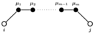
Figure 1: A path connecting the measured nodes $i$ and $j$ (open circles) via the hidden nodes $\mu_{1},\mu_{2},\ldots,\mu_{m-1},\mu_{m}$ (closed circles).

As indicated by Eq. (8), the distribution of the off-diagonal elements of $\Sigma^{-1}_{ij}$ for $i,j=1,2,\ldots,n$ can be written as

$$P(\Sigma^{-1}_{ij}=x)=(1-r)P_{0}(x)+rP_{1}(x)$$ (26)

where $r$ is the fraction of connected pairs among the measured nodes and is equal to the number of connected pairs of measured nodes divided by $n(n-1)/2$, $P_{0}$ and $P_{1}$ are the distributions of $\Sigma^{-1}_{ij}$ with $A_{ij}=0$ and $A_{ij}=1$ respectively. If the positive and negative coupling strength of the links are described by two different distributions, $P_{1}$ can further be a mixture of two distributions $P_{1+}$ and $P_{1-}$, which correspond to $g_{ij}>0$ and $g_{ij}<0$ respectively [c.f. Eq. (48)]. In the limit of infinite number of data, $P_{0}(x)$ approaches $\delta(x)$. For a finite number of data points, numerical studies correlated show that $P_{0}(x)$ is well-approximated by a Gaussian distribution of mean $m_{0}=0$ and standard deviation $\sigma_{0}$, and $\sigma_{0}$ decreases when the number of data points increases. Equation (8) implies that $P_{1}(x)$ would have a mean $m_{1}$ and standard deviation $\sigma_{1}$ given by

$$m_{1}=-\frac{2}{\sigma_{n}^{2}}\langle g\rangle\ ;\qquad\sigma_{1}=\frac{2}{\sigma_{n}^{2}}\sigma_{g}$$ (27)

where $\langle g\rangle$ and $\sigma_{g}$ are the average and standard deviation of the coupling strength $g_{ij}$ of the links. In the presence of hidden nodes, the corrections $C_{ij}$ will modify the distributions $P_{0}$ and $P_{1}$ to ${\tilde{P}}_{0}$ and ${\tilde{P}}_{1}$:

$$P((\Sigma_{m}^{-1})_{ij}=x)=(1-r){\tilde{P}}_{0}(x)+r{\tilde{P}}_{1}(x)\ ,\ \ i\neq j$$ (28)

The mean and standard deviation of ${\tilde{P}}_{i}$, denoted by $\tilde{m}_{i}$, $\tilde{\sigma}_{i}$, $i=0$ and $1$, would be modified. Using Eq. (21) and the results for $P_{0}(x)$, we obtain

$${\tilde{m}}_{0} = -\frac{2}{\sigma_{n}^{2}}\mu_{C,0}$$ (29)

$${\tilde{\sigma}}_{0}^{2} \approx \sigma_{0}^{2}+\frac{4}{\sigma_{n}^{4}}\sigma_{C,0}^{2}$$ (30)

$${\tilde{m}}_{1} = m_{1}-\frac{2}{\sigma_{n}^{2}}\mu_{C,1}$$ (31)

$${\tilde{\sigma}}_{1}^{2} = \sigma_{1}^{2}+\frac{4}{\sigma_{n}^{4}}\left[\sigma_{C,1}^{2}+K(g_{ij},C_{ij})\right]\ \$$ (32)

where

$$\mu_{C,0} \equiv \langle C_{ij}|A_{ij}=0\rangle$$ (33)

$$\mu_{C,1} \equiv \langle C_{ij}|A_{ij}=1\rangle$$ (34)

$$\sigma_{C,0}^{2} \equiv \langle C_{ij}^{2}|A_{ij}=0\rangle-\langle C_{ij}|A_{ij}=0\rangle^{2}$$ (35)

$$\sigma_{C,1}^{2} \equiv \langle C_{ij}^{2}|A_{ij}=1\rangle-\langle C_{ij}|A_{ij}=1\rangle^{2}$$ (36)

$$K(g_{ij},C_{ij}) \equiv \langle g_{ij}C_{ij}|A_{ij}=1\rangle-\langle g\rangle\langle C_{ij}|A_{ij}=1\rangle\qquad$$ (37)

Here $\mu_{C,i}$ and $\sigma_{C,i}$ for $i=1,2$ are the conditional average and conditional standard deviation of $C_{ij}$ for $A_{ij}=0$ and $A_{ij}=1$ respectively, and $K(g_{ij},C_{ij})$ measures the correlation of $C_{ij}$ with the coupling strength $g_{ij}$ for measured nodes $i$ and $j$ that are connected. Hence, the corrections $C_{ij}$ would shift the means, broaden and distort the distributions of $P_{0}$ and $P_{1}$ to $\tilde{P}_{0}$ and $\tilde{P}_{1}$.

Suppose $P_{0}$ and $P_{1}$ are distinguishable. If ${\tilde{P}}_{0}$ and ${\tilde{P}}_{1}$ remain distinguishable even though with a larger extent of overlap, then the links among the measured nodes can still be reconstructed amid with a larger error rate. For a mixture of two general distributions, there is no simple criterion on when the component distributions are distinguishable. Nonetheless, the component distributions are likely to be distinguishable when the absolute value of the difference between their means are larger than a certain multiple of the sum of their standard deviations. Let $m_{1}-m_{0}=\gamma(\sigma_{0}+\sigma_{1})$ with $|\gamma|>1$. Using Eqs. (29)-(32), we obtain

$${\tilde{m}}_{1}-{\tilde{m}}_{0}$$ (38)

$$= \gamma\left\{({\tilde{\sigma}}_{0}^{2}-\frac{4}{\sigma_{n}^{2}}{\sigma_{C,0}^{2})^{1/2}+[{\tilde{\sigma}}_{1}^{2}-\frac{4}{\sigma_{n}^{2}}(\sigma_{C,1}^{2}+K)]^{1/2}}\right\}$$

$$\ \ -\frac{2}{\sigma_{n}^{2}}(\mu_{C,1}-\mu_{C,0})$$

Thus ${\tilde{P}}_{0}$ and ${\tilde{P}}_{1}$ are likely to remain distinguishable (with $|{\tilde{m}}_{1}-{\tilde{m}}_{0}|/({\tilde{\sigma}}_{0}+{\tilde{\sigma}}_{1})>1$) if $|\mu_{C,1}-\mu_{C,0}|$, $\sigma_{C,0}$, $\sigma_{C,1}$ and $|K(g_{ij},C_{ij})|$ are sufficiently small.

To shed further light on this, we use Eq. (20) to obtain a crude estimate of $C_{ij}$. Substitute ${\bm{L}}_{h}+a{\bm{I}}_{n_{h}}={\bm{S}}-{\bm{W}}={\bm{S}}({\bm{I}}_{n_{h}}-{\bm{S}}^{-1}{\bm{W}})$ into Eq. (20), we have

$${\bm{C}}={\bm{E}}({\bm{I}}_{n_{h}}-{\bm{S}}^{-1}{\bm{W}})^{-1}{\bm{S}}^{-1}{\bm{E}}^{T}$$ (39)

If the Neumann series $\sum_{k=0}^{\infty}({\bm{S}}^{-1}{\bm{W}})^{k}$ converges, it converges to $({\bm{I}}_{n_{h}}-{\bm{S}}^{-1}{\bm{W}})^{-1}$. The necessary and sufficient condition for the Neumann series to converge is the spectral radius of ${\bm{S}}^{-1}{\bm{W}}$, denoted by $\rho({\bm{S}}^{-1}{\bm{W}})$, is less than 1 note . For networks with $g_{ij}\geq 0$, one can easily show that the infinity norm $||{\bm{S}}^{-1}{\bm{W}}||_{\infty}\equiv\max_{\mu}\{\sum_{\nu}|({\bm{S}}^{-1}{\bm{W}})_{\mu\nu}|\}<1$, and thus $\rho({\bm{S}}^{-1}{\bm{W}})\leq||{\bm{S}}^{-1}{\bm{W}}||_{\infty}<1$. For networks with both positive and negative $g_{ij}$, we have checked numerically that $\rho({\bm{S}}^{-1}{\bm{W}})<1$ for all the cases studied. When the Neumann series converges, we keep two terms in the series, namely $({\bm{I}}_{n_{h}}-{\bm{S}}^{-1}{\bm{W}})^{-1}\sim{\bm{I}}_{n_{h}}+{\bm{S}}^{-1}{\bm{W}}$, to obtain a crude estimate of $C_{ij}$:

$$C_{ij} \sim \sum_{\mu=n+1}^{N}\frac{g_{i\mu}g_{j\mu}A_{i\mu}A_{j\mu}}{s_{\mu}+a}$$ (40)

$$+\sum_{\mu,\nu=n+1}^{N}\frac{g_{i\mu}g_{\mu\nu}g_{j\nu}A_{i\mu}A_{\mu\nu}A_{j\nu}}{(s_{\mu}+a)(s_{\nu}+a)}$$

Using Eq. (40), one sees that the magnitude of $C_{ij}$ depends on three factors: (1) the number of paths connecting the measured nodes $i$ and $j$ via the hidden nodes which determines the number of nonzero terms in the sums, (2) the strength of the hidden nodes and (3) the coupling strength of the links in these paths. Regarding to the second factor, we note that hidden nodes with larger strength actually give rise to smaller corrections in contrary to what one might have guessed. If these factors do not differ much between the two groups of unconnected or connected measured nodes, then $\mu_{C,1}\sim\mu_{C,0}$; if these factors do not vary much among the measured nodes in each group, then $\sigma_{C,0}$ and $\sigma_{C,1}$ would be small and if these factors do not correlate with the magnitude of $g_{ij}$ for connected measured nodes, then $|K(g_{ij},C_{ij})|$ would be small even when the magnitudes of the corrections $C_{ij}$’s themselves might be large. Such situations are expected when the the hidden nodes are not preferentially linked to the measured nodes in any manner. In this case, ${\tilde{P}}_{0}$ and ${\tilde{P}}_{1}$ remain distinguishable and it is possible to reconstruct the links among the measured nodes from $(\Sigma_{m}^{-1})_{ij}$, $i\neq j$.

V Numerical results and discussions

We check our theoretical results using data from numerical simulations. We study five different networks, four of $N=100$ each and one of $N=1000$.

• Network A: it consists of two random networks, each of 50 nodes and a connection probability of 0.2, connected to each other by one link and $g_{ij}$’s, taken from a Gaussian distribution $\mathcal{N}(10,2^{2})$ of mean 10 and standard deviation 2, are all positive. We take all the 50 nodes of one of the random network as hidden nodes.

• Network B: it is a random network of connection probability 0.2 and $g_{ij}$’s also taken from $\mathcal{N}(10,2^{2})$ and are all positive. We choose the hidden nodes randomly from the network with $n_{h}\leq 70$ such that the number of links among the measured nodes is at least of the order of 100.

• Network C: it is similar to network B except that $g_{ij}$ of 80% of the links taken from $\mathcal{N}(10,2^{2})$ and the remaining 20% taken from $\mathcal{N}(-10,2^{2})$. As a result, about 80% of the $g_{ij}$’s are positive and about 20% are negative. The hidden nodes are chosen randomly from the network.

• Network D: it is a scale-free network of $N=1000$ BA with degree distribution obeying a power law and $g_{ij}$’s taken from $\mathcal{N}(10,2^{2})$ are all positive. The hidden nodes are chosen randomly from the network.

• Network E: it is constructed by linking 30 additional nodes to a random network of $70$ nodes and connection probability 0.2 with the restriction that every one of the additional nodes is only commonly connected to randomly selected pairs of unconnected nodes in the random network; and the additional nodes are randomly connected among themselves with the same connection probability 0.2. $g_{ij}$’s are taken from $\mathcal{N}(10,2^{2})$ and are all positive. We take the 30 additional nodes as hidden nodes.

For the dynamics, we mainly study nonlinear logistic function

$$f(x)=10x(1-x)$$ (41)

and diffusive coupling function

$$h(y-x)=y-x$$ (42)

and take $\sigma_{n}=1$ for the noise. To explore how general our theoretical results are, we go beyond the description by Eq. (2) and study two additional cases. In the first additional case, the nodes of network B have two-dimensional state variables $(x_{i}(t),y_{i}(t))$ with nonlinear FitzHugh-Nagumo (FHN) dynamics FHN

$$\dot{x_{i}} = (x_{i}-{x_{i}^{3}}/{3}-y_{i})/\epsilon+\displaystyle\sum\limits_{j\neq i}g_{ij}A_{ij}(x_{j}-x_{i})+\eta_{i}\qquad$$ (43)

$$\dot{y_{i}} = x_{i}+\alpha\,$$ (44)

where $\epsilon=0.01$ and $\alpha=0.95$. In the second additional case, the nodes of network B have three-dimensional state variables $(x_{i}(t),y_{i}(t),z_{i}(t))$ with nonlinear Rössler dynamics Rossler and nonlinear coupling PRErapid :

$$\dot{x}_{i} = -y_{i}-z_{i}+\sum_{j\neq i}g_{ij}A_{ij}\tanh(x_{j}-x_{i})+\eta_{i}$$ (45)

$$\dot{y}_{i} = x_{i}+c_{1}y_{i}+\sum_{j\neq i}g_{ij}A_{ij}\tanh(y_{j}-y_{i})$$ (46)

$$\dot{z}_{i} = c_{2}+z_{i}(x_{i}-c_{3})+\sum_{j\neq i}g_{ij}A_{ij}\tanh(z_{j}-z_{i})\ \qquad$$ (47)

where $c_{1}=c_{2}=0.2$ and $c_{3}=9$. In these two additional cases, the system does not approach a steady state in the absence of noise, and has chaotic dynamics when the nodes are decoupled in the second case with Rössler dynamics. We integrate the equations of motion using the Euler-Maruyama method and record the time series $x_{i}(t)$ with a sampling interval $\delta t=5\times 10^{-4}$. For all the cases studied, including the cases with FHN and Rössler dynamics, we calculate ${\bm{\Sigma}}$ using $x_{i}(t)$’s with a time average over $N_{\rm data}=2\times 10^{6}$ data points.

For network A, since there is only one link connecting the hidden nodes and the measured nodes, there is no path connecting any pair of measured nodes via the hidden nodes thus $C_{ij}=0$ for all $i\neq j$. As a result, Eq. (22) implies that $(\Sigma_{m}^{-1})_{ij}=\Sigma_{ij}^{-1}$ for $i\neq j$. We show the distributions of $P(\Sigma_{ij}^{-1})$ and $P((\Sigma_{m}^{-1})_{ij})$ for $i\neq j=1,2,\ldots,n=50$ in Fig. 2. As expected, the two distributions coincide with each other. Moreover, $P(\Sigma_{ij}^{-1})$ is bimodal with the peak around zero corresponding to $P_{0}$ for unconnected nodes and the peak around $x_{m}\approx-20$ corresponding to $P_{1}$ for connected nodes in accord with Eq. (26). Furthermore, the value of $x_{m}$ is in excellent agreement with the theoretical value of $\mu_{1}=-2\langle g\rangle/\sigma_{n}^{2}$ [see Eq. (27)]. Hence in this case, the links among the measured nodes can be reconstructed from $(\Sigma_{m}^{-1})_{ij}$ with $i\neq j$, which can be calculated using the dynamics $y_{i}(t)$ of the measured nodes only.

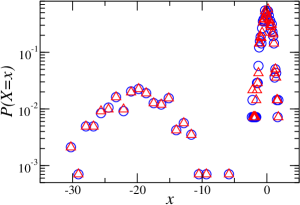
Figure 2: Comparison of the distributions $P(X=x)$ of $X=\Sigma^{-1}_{ij}$ (circles) and $X=(\Sigma_{m}^{-1})_{ij}$ (triangles) for $i\neq j=1,2,\ldots,n=50$ for network A.

For network B with the hidden nodes randomly chosen, there are nonzero $C_{ij}$’s for some pairs of measured nodes $i$ and $j$. We first consider the case with logistic dynamics and calculate $C_{ij}$ using Eq. (20) and together with ${\Sigma}^{-1}_{ij}$, we obtain the theoretical results for $(\Sigma_{m}^{-1})_{ij}$ using Eq. (22). We compare these theoretical results with $(\Sigma_{m}^{-1})_{ij}$ directly calculated from the measured dynamics $y_{i}(t)$’s in Fig. 3 and perfect agreement is found for all the values of $n_{h}$ studied. For FHN and Rössler dynamics, the system is not described by Eq. (2) thus $a=-f^{\prime}(X_{0})$ is not defined. We put $a=0$ in Eq. (20) and obtain the theoretical estimate for the off-diagonal $(\Sigma_{m}^{-1})_{ij}$ as $\Sigma^{-1}_{ij}-(2/\sigma_{n}^{2})(EL_{h}^{-1}E^{T})_{ij}$. Interestingly, these theoretical estimates are in good agreement with the directly calculated $(\Sigma_{m}^{-1})_{ij}$’s in most cases, as shown in Figs. 4 and 5. For FHN dynamics with larger $n_{h}$, an improved theoretical estimate is obtained by $\Sigma^{-1}_{ij}-(2/\sigma_{n}^{2})[(EL_{h}^{-1}E^{T})_{ij}+b]$, where $b$ is a constant. This indicates the general applicability of our theoretical results beyond the model class studied.

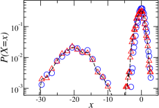
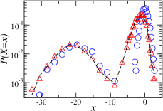
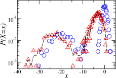
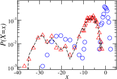
Figure 3: Comparison of distributions $P(X=x)$ of $X=\Sigma^{-1}_{ij}$ (circles) and $X=(\Sigma_{m}^{-1})_{ij}$ (triangles) for network B with logistic dynamics and different number of hidden nodes: (a) $n_{h}=10$, (b) $n_{h}=30$, (c) $n_{h}=50$, and (d) $n_{h}=70$. The dashed lines are the theoretical results of $X=\Sigma^{-1}_{ij}-2C_{ij}/\sigma_{n}^{2}$ with $C_{ij}$ calculated using Eq. (20).

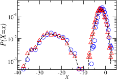
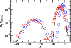
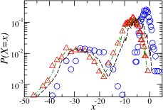
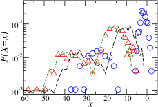
Figure 4: Same as Fig. 3 for network B with FHN dynamics but the dashed lines are now the theoretical estimates of $X=\Sigma^{-1}_{ij}-(2/\sigma_{n}^{2})(EL_{h}^{-1}E^{T})_{ij}$. The dot-dashed lines are the improved theoretical estimates of $X=\Sigma^{-1}_{ij}-(2/\sigma_{n}^{2})[(EL_{h}^{-1}E^{T})_{ij}+b]$ with $b=1$ for (c) and $b=3$ for (d).

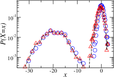
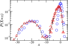
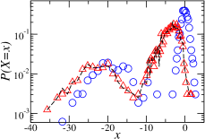
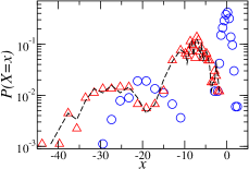
Figure 5: Same as Fig. 4 for network B with Rössler dynamics.

As shown in Figs. 3-5, the distribution $P((\Sigma_{m}^{-1})_{ij})$ is a mixture of the modified distributions $\tilde{P}_{0}$ and $\tilde{P}_{1}$, in accord with Eq. (28), which remain distinguishable as expected since the hidden nodes are chosen randomly. Thus it is possible to reconstruct the links among the measured nodes from $(\Sigma_{m}^{-1})_{ij}$ with $i\neq j$. We note that this is true for all the three kinds of dynamics studied and even when the hidden nodes outnumber the measured nodes. In Table 1, we compare the error rates of the reconstruction results obtained using k-means clustering of $(\Sigma_{m}^{-1})_{ij}$ from the measured dynamics only and of ${\Sigma}^{-1}_{ij}$ from the dynamics of the whole network. We measure the error rates by the ratios of false negatives (FN) and false positives (FP) over the number of actual links $N_{L}$ among the measured nodes. These error rates are related to the sensitivity and specificity usually used for a predictive test: sensitivity is given by $1-{\rm FN}/N_{L}$ and specificity is given by $1-({\rm FP}/N_{L})\rho/(1-\rho)$, where $\rho=N_{L}/[n(n-1)/2]$ is the link density of the measured nodes. For networks with low link density $\rho$, the error rates can be rather high even when specificity is close to 1 so the error rates are better measures of the accuracy of the reconstruction results PRErapid2 . As can be seen, the accuracy of the reconstruction results using $(\Sigma_{m}^{-1})_{ij}$ from the measured nodes only is comparable to that obtained using $(\Sigma^{-1})_{ij}$ from all the nodes.

network	dynamics	$n_{h}$	$\rho$	FN/$N_{L}$ (%)	FP/$N_{L}$ (%)
A	logistic	$50$	0.202	0.81 (0.81)	0.00 (0.00)
B	logistic	$10$	0.198	$0.76\;\;(0.88)$	$0.00\;\;(0.00)$
		$30$	0.197	$1.05\;\;(1.26)$	$0.00\;\;(0.00)$
		$50$	0.202	$1.62\;\;(1.62)$	$0.00\;\;(0.00)$
		$70$	0.218	$1.05\;\;(3.16)$	$0.00\;\;(0.00)$
	FHN	$10$	0.198	$0.63\;\;(0.51)$	$0.00\;\;(0.00)$
		$30$	0.197	$1.05\;\;(0.84)$	$0.00\;\;(0.00)$
		$50$	0.202	$1.62\;\;(1.21)$	$0.00\;\;(0.00)$
		$70$	0.218	$3.16\;\;(1.05)$	$1.05\;\;(0.00)$
	Rössler	$10$	0.198	$1.01\;\;(0.88)$	$0.00\;\;(0.00)$
		$30$	0.197	$1.10\;\;(0.44)$	$0.00\;\;(0.00)$
		$50$	0.202	$0.87\;\;(1.31)$	$0.00\;\;(0.00)$
		$70$	0.218	$3.57\;\;(0.00)$	$5.95\;\;(0.00)$
C	logistic	$20$	0.198	$0.96\;\;(0.80)$	$0.00\;\;(0.00)$
		$30$	0.197	$0.85\;\;(0.21)$	$0.00\;\;(0.00)$
		$40$	0.199	$0.85\;\;(0.00)$	$1.14\;\;(0.00)$
		60	0.206	2.48 (0.00)	1.86 (0.00)
D	logistic	100	0.0039	0.44 (0.50)	0.00 (0.00)
		300	0.0037	0.45 (0.45)	0.11 (0.00)
		500	0.0040	0.60 (0.60)	1.20 (0.00)
		700	0.0017	1.05 (1.05)	3.16 (0.00)
E	logistic	$30$	0.199	$0.42\;\;(0.42)$	$29.88\;(0.00)$

Table 1: Error rates of the reconstruction results using k-means clustering of $(\Sigma_{m}^{-1})_{ij}$ for the various networks studied. $N=100$ for networks A, B, C and E and $N=1000$ for network D. $\rho=N_{L}/[n(n-1)/2]$, where $N_{L}$ is the number of links among the measured nodes and $n=N-n_{h}$ is the number of measured nodes. Two clusters are used for all networks except network C where three clusters are used. We show also the error rates using $\Sigma^{-1}_{ij}$ in parentheses.

For network C, the positive and negative $g_{ij}$’s follow two different distributions so $P_{1}$ can be further decomposed into a weighted sum of $P_{1+}$ and $P_{1-}$, which correspond to $g_{ij}>0$ and $g_{ij}<0$ respectively. Therefore, Eq. (26) can be rewritten as

$$P(\Sigma^{-1}_{ij}=x)$$ (48)

$$= (1-r)P_{0}(x)+r[\beta P_{1+}(x)+(1-\beta)P_{1-}(x)]\qquad$$

where $\beta$ is the fraction of the links among the measured nodes with positive $g_{ij}$’s. Similarly, Eq. (28) is also rewritten as

$$P((\Sigma_{m}^{-1})_{ij}=x)$$ (49)

$$= (1-r)\tilde{P}_{0}(x)+r[\beta\tilde{P}_{1+}(x)+(1-\beta)\tilde{P}_{1-}(x)]\qquad$$

As $g_{ij}$ can now be either positive or negative, the terms in the summations contributing to $C_{ij}$ [see Eq. (40)] could cancel one another. Thus we expect the magnitudes of $\mu_{C,0}$, $\mu_{C,1+}\equiv\langle C_{ij}|A_{ij}=1,g_{ij}>0\rangle$ and $\mu_{C,1-}\equiv\langle C_{ij}|A_{ij}=1,g_{ij}<0\rangle$ to be smaller than the magnitudes of $\mu_{C,0}$ and $\mu_{C,1}$ for network B with logistic dynamics. It can indeed be clearly seen that the shifts of $\tilde{P}_{0}$, $\tilde{P}_{1+}$ and $\tilde{P}_{1-}$ from $P_{0}$, $P_{1+}$ and $P_{1-}$ in Fig. 6 are smaller than the shifts of $\tilde{P}_{0}$ and $\tilde{P}_{1}$ from $P_{0}$ and $P_{1}$ in Fig. 3. Moreover, $\tilde{P}_{0}$, $\tilde{P}_{1+}$ and $\tilde{P}_{1-}$ are again only slightly broadened as compared with $P_{0}$, $P_{1+}$ and $P_{1-}$ because the hidden nodes are randomly chosen. Thus for network C, the links among the measured nodes can also be accurately reconstructed from clustering of $(\Sigma_{m}^{-1})_{ij}$ with $i\neq j$ (see Table 1).

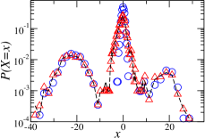
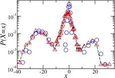
Figure 6: Similar to Fig. 3 for network C with both positive and negative $g_{ij}$’s for two different numbers of hidden nodes: (a) $n_{h}=20$ and (b) $n_{h}=40$.

For the scale-free network D, as the link density $\rho$ is very small, most of the measured nodes are not linked via a path of hidden nodes and thus most $C_{ij}$’s vanish. But as the nodes have a power-law degree distribution, both the strength of the hidden nodes and the number of paths connecting measured nodes via hidden nodes could have a large variation leading to a large variation in the magnitude of $C_{ij}$’s. This implies a large $\sigma_{C,0}/\mu_{C,0}$ and $\sigma_{C,1}/\mu_{C,1}$ as compared to the case of random network B. In particular, this results in a larger distortion from $P_{0}$ to ${\tilde{P}}_{0}$ as seen in Fig. 7. The effect is more evident for $P_{0}$ because there are far more unconnected measured nodes than connected measured nodes due to the small $\rho$. Nonetheless, ${\tilde{P}}_{0}$ and ${\tilde{P}}_{1}$ remain distinguishable and the error rates of the reconstruction of the links among the measured nodes remain low (see Table 1).

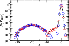
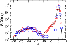
Figure 7: Similar to Fig. 3 for scale-free network D with (a) $n_{h}=100$ and (b) $n_{h}=700$.

In network E, every one of the $n_{h}=30$ hidden nodes is only commonly linked to randomly selected pairs of unconnected measured nodes. We first randomly choose a pair of unconnected measured nodes and link all the $n_{h}$ hidden nodes to both of them. Then we link the hidden nodes to a second pair of unconnected measured nodes with the restriction that no hidden nodes are commonly linked to connected measured nodes that might exist among the first and second pairs of unconnected nodes. Therefore, the number of hidden nodes commonly linked to the second pair can be less than $n_{h}$. We repeat the process for all the remaining pairs of unconnected measured nodes. In this way, the number of hidden nodes commonly linked to a given pair of measured nodes $i$ and $j$ or the number of nonzero terms in the first sum in Eq. (40) is identically zero for $i$ and $j$ that are connected, and varies among $i$ and $j$ that are unconnected. This preferential connection of the hidden nodes to unconnected measured nodes gives rise to $\mu_{C,0}>\mu_{C,1}$ and $\sigma_{C,0}>\sigma_{C,1}$. Thus the distortion of $P_{0}$ is large leading to a larger overlap of $\tilde{P}_{0}$ and $\tilde{P}_{1}$ as shown in Fig. 8. As expected, the error rates of the reconstruction results are larger with FP/$N_{L}\approx 30$% (see Table 1). However, we note that even with this error rate, the specificity is above 90%. Moreover, the error rate FN/$N_{L}$ remains less than 1% and thus more than 99% of the actual links among the measured nodes are correctly reconstructed.

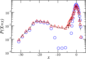
Figure 8: Comparison of distributions $P(X=x)$ of $X=\Sigma^{-1}_{ij}$ (circles) and $X=(\Sigma_{m}^{-1})_{ij}$ (triangles) for network E with $n_{h}=30$ hidden nodes that are preferentially linked to measured nodes that are unconnected. The dashed line is the theoretical result of $X=\Sigma^{-1}_{ij}-2C_{ij}/\sigma_{n}^{2}$ with $C_{ij}$ calculated using Eq. (20).

VI Conclusions

We have addressed the interesting question of how hidden nodes affect reconstruction of bidirectional networks. By using a model class of bidirectional networks with nonlinear dynamics and diffusive-like coupling and subjected to a Gaussian white noise, as described by Eq. (2), we have derived analytical results, Eqs. (19) and Eq. (22), that allow us to answer this question precisely. Hidden nodes affect the reconstruction results by introducing corrections $C_{ij}$. These corrections $C_{ij}$ are nonzero when the measured nodes $i$ and $j$ are connected via a path of hidden nodes as depicted in Fig. 1. Our estimate of $C_{ij}$, as shown in Eq. (40), shows that three factors determine $C_{ij}$’s, namely the number of paths of hidden nodes connecting the two measured nodes $i$ and $j$, the coupling strength of the links and the strength of the hidden nodes in these paths. Interestingly, hidden nodes with larger strength give rise to smaller corrections when the other two factors remain the same. When the hidden nodes are not preferentially linked to the measured nodes in any manner, these three factors would not differ much between or among the two groups of connected and unconnected measured nodes and, as a result, the hidden nodes would have little effects on the reconstruction of the links among the measured nodes. This is true even when the hidden nodes outnumber the measured nodes. In the event that the hidden nodes are preferentially linked to the measured nodes such that one or more of the above three factors vary significantly either between or among the two groups, the accuracy of the reconstruction results would deteriorate. Yet useful information can still be uncovered. We have verified our theoretical results and their implications using numerical simulations and our numerical results indicate the applicability of our results and analytical understanding beyond the model class of bidirectional networks studied.

Hence our work shows that the method based on the inverse of covariance is useful for reconstructing bidirectional networks even when there are hidden nodes. Most networks of interest in real-world problems are directed. It is highly challenging to derive analytical results for the effects of hidden nodes on the reconstruction of general directed networks. It would thus be interesting to investigate whether and how the present results and understanding for bidirectional networks can be extended to general directed networks.

Appendix A Derivation of Eq. (25)

Denote the eigenvalues of $\bm{M}\equiv\bm{L}_{h}+a{\bm{I}}_{n_{h}}$ by $\lambda_{k}$, $k=1,\ldots,n_{h}$. By Cayley-Hamilton theorem, $\bm{M}$ satisfies its own characteristic equation. Therefore

$$\bm{0} = \prod_{k=1}^{N-n}(\bm{M}-\lambda_{k}\bm{I}_{n_{h}})$$ (50)

$$= \bm{M}^{n_{h}}+\sum_{m=1}^{n_{h}}(-1)^{m}e_{m}\bm{M}^{n_{h}-m}\qquad$$

where ${\bm{M}}^{0}=\bm{I}_{n_{h}}$ and $e_{m}(\lambda_{1},\ldots,\lambda_{k})$, $1\leq m\leq n_{h}$, are the elementary symmetric polynomials of $\lambda_{k}$’s. For example, $e_{1}=\sum_{k=1}^{n_{h}}\lambda_{k}$ and $e_{n_{h}}=\prod_{k=1}^{n_{h}}\lambda_{k}$. Multiplying ${\bm{M}}^{-1}$ to Eq. (50) and rearranging terms, we express ${\bm{M}}^{-1}$ as a finite polynomial of $\bm{M}$:

$${\bm{M}}^{-1} = \sum_{m=0}^{n_{h}-1}(-1)^{m}\frac{e_{n_{h}-1-m}}{e_{n_{h}}}\bm{M}^{m}\qquad$$ (51)

Using $\bm{M}\equiv\bm{S}-\bm{W}$ with $\bm{S}$ and $\bm{W}$ defined in Eqs. (23) and (24), we obtain the elements of ${\bm{M}}^{m}$ in terms of the elements of $\bm{S}$ and $\bm{W}$. For $m=1$ and $2$:

$$M_{\mu\nu} = f_{0}^{(1)}\delta_{\mu\nu}+f^{(1)}_{1}W_{\mu\nu}$$ (52)

$$(M^{2})_{\mu\nu} = f_{0}^{(2)}\delta_{\mu\nu}+f^{(2)}_{1}W_{\mu\nu}+\sum_{\alpha=1}^{n_{h}}f^{(2)}_{2}W_{\mu\alpha}W_{\alpha\nu}\qquad$$ (53)

and for $3\leq m\leq n_{h}-1$:

$$(M^{m})_{\mu\nu}=f^{(m)}_{0}\delta_{\mu\nu}+f^{(m)}_{1}W_{\mu\nu}+\sum_{\alpha=1}^{n_{h}}f^{(m)}_{2}W_{\mu\alpha}W_{\alpha\nu}$$

$$+\sum_{k=3}^{m}\sum_{\alpha_{1},\cdots,\alpha_{k-1}=1}^{n_{h}}f^{(m)}_{k}W_{\mu\alpha_{1}}\left(\prod_{j=1}^{k-2}W_{\alpha_{j}\alpha_{j+1}}\right)W_{\alpha_{k-1}\nu}\qquad\ \$$ (54)

Here $f^{(m)}_{0}=(s_{\mu+n}+a)^{m}$ and $f^{(m)}_{m}=(-1)^{m}$ for $m=1,\ldots,n_{h}-1$. For $m\geq 2$, $f^{(m)}_{k}$, $1\leq k\leq m-1$, generally depends on $\hat{s}_{\mu+n}\equiv{s}_{\mu+n}+a$, $\hat{s}_{\nu+n}$ and $\hat{s}_{\alpha_{i}+n}$, $i=1,\ldots,k-1$. Explicit results for $f^{(m)}_{k}$, $1\leq k\leq m-1$, for $m=2$ and 3 are

$$f^{(2)}_{1} = -(\hat{s}_{\mu+n}+\hat{s}_{\nu+n})$$ (55)

$$f^{(3)}_{1} = -[(\hat{s}_{\mu+n})^{2}+(\hat{s}_{\nu+n})^{2}+\hat{s}_{\mu+n}\hat{s}_{\nu+n}]$$ (56)

$$f^{(3)}_{2} = \hat{s}_{\mu+n}+\hat{s}_{\nu+n}+\hat{s}_{\alpha+n}$$ (57)

Substituting Eqs. (52)-(54) into Eq. (51), we obtain

$$(M^{-1})_{\mu\nu}=F_{0}\delta_{\mu\nu}+F_{1}W_{\mu\nu}+\sum_{\alpha=1}^{n_{h}}F_{2}W_{\mu\alpha}W_{\alpha\nu}$$

$$+\sum_{k=3}^{n_{h}-1}\sum_{\alpha_{1},\cdots,\alpha_{k-1}=1}^{n_{h}}F_{k}W_{\mu\alpha_{1}}\left(\prod_{j=1}^{k-2}W_{\alpha_{j}\alpha_{j+1}}\right)W_{\alpha_{k-1}\nu}\qquad$$ (58)

where

$$F_{k}=\sum_{m=k}^{n_{h}-1}(-1)^{m}\frac{e_{n_{h}-1-m}}{e_{n_{h}}}f_{k}^{(m)},\ \ \ 0\leq k\leq n_{h}-1,$$ (59)

depends generally on $\hat{s}_{\mu+n}$, $\hat{s}_{\nu+n}$, $\hat{s}_{\alpha_{i}+n}$, $i=1,\ldots,k-1$ and $\lambda_{k}$. Putting Eq. (58) into Eq. (20), we thus obtain

$$C_{ij}=\sum_{\mu,\nu=1}^{n_{h}}E_{i\mu}(M^{-1})_{\mu\nu}E_{j\nu}$$

$$=\sum_{\mu_{1}=1}^{n_{h}}F_{0}W_{i\mu_{1}}W_{\mu_{1}j}+\sum_{\mu_{1},\mu_{2}=1}^{n_{h}}F_{1}W_{i\mu_{1}}W_{\mu_{1}\mu_{2}}W_{\mu_{2}j}$$

$$+\sum_{k=3}^{n_{h}-1}\sum_{\mu_{1},\cdots,\mu_{k+1}=1}^{n_{h}}F_{k}W_{i\mu_{1}}\left(\prod_{j=1}^{k}W_{\mu_{j}\mu_{j+1}}\right)W_{\mu_{k+1}j}\qquad\qquad$$ (60)

which is just Eq. (25).

References

- (1) S.H. Strogatz, Exploring complex networks, Nature (London) 410, 268 (2001).
- (2) M. Timme, Does dynamics reflect topology in directed networks?, Europhys. Lett. 76, 367 (2006).
- (3) M. Timme and J. Casadiego, Revealing networks from dynamics: an introduction, J. Phys. A 47, 343001 (2014).
- (4) W.-X. Wang, Y.-C. Lai, C. Grebogi, Data based identification and prediction of nonlinear and complex dynamical systems, Phys. Reports 644, 1 (2016).
- (5) J. Ren, W.-X. Wang, B. Li, and Y.-C. Lai, Noise Bridges Dynamical Correlation and Topology in Coupled Oscillator Networks, Phys. Rev. Lett. 104, 058701 (2010).
- (6) E.S.C. Ching, P.Y. Lai, and C.Y. Leung, Extracting connectivity from dynamics of networks with uniform bidirectional coupling, Phys. Rev. E 88, 042817 (2013); Erratum, Phys. Rev. E 89, 029901(E) (2014).
- (7) E.S.C. Ching, P.Y. Lai, and C.Y. Leung, Reconstructing weighted networks from dynamics, Phys. Rev. E 91, 030801(R) (2015).
- (8) Z. Zhang, Z. Zheng, H. Niu, Y. Mi, S. Wu, and G. Hu, Solving the inverse problem of noise-driven dynamic networks, Phys. Rev. E 91, 012814 (2015).
- (9) E.S.C. Ching and H.C. Tam, Reconstructing links in directed networks from noisy dynamics, Phys. Rev. E 95, 010301(R) (2017).
- (10) P.Y. Lai, Reconstructing Network topology and coupling strengths in directed networks of discrete-time dynamics, Phys. Rev. E 95, 022311 (2017).
- (11) Y. Chen, S. Wang, Z. Zheng, Z. Zhang and G. Hu, Depicting network structures from variable data produced by unknown colored-noise driven dynamics, Europhys. Lett. 113, 18005 (2016).
- (12) H.C. Tam, E.S.C. Ching, and P.Y. Lai, Reconstructing networks from dynamics with correlated noise, Physica A 502, 106 (2018).
- (13) B. Dunn and Y. Roudi, Learning and inference in a nonequilibrium Ising model with hidden nodes, Phys. Rev. E 87, 022127 (2013).
- (14) R.-Q. Su, Y.-C. Lai, X. Wang, and Y. Do, Uncovering hidden nodes in complex networks in the presence of noise, Sci. Reports 4, 3944 (2014).
- (15) Y.H. Chang and C.J. Tomlin, Reconstruction of Gene Regulatory Networks with Hidden Nodes, Proc. Eur. Control Conf., 1492 (2014).
- (16) X. Han, Z. Shen, W.-X. Wang, and Z. Di, Robust Reconstruction of Complex Networks from Sparse Data, Phys. Rev. Lett. 114, 028701 (2015).
- (17) H. Huang, Effects of hidden nodes on network structure inference, J. Phys. A: Math. Theor. 48, 355002 (2015).
- (18) Y. Chen, C. Zhang, T.Y. Chen, S. Wang, and G. Hu, Reconstruction of noise-driven dynamic networks with some hidden nodes, Sci. China Phys. Mech. Astron. 60, 070511 (2017).
- (19) J. Casadiego, M. Nitzan, S. Hallerberg, and M. Timme, Model-free inference of direct network interactions from nonlinear collective dynamics, Nature Commun. 8, 2192 (2017).
- (20) J.M. Stuart, E. Segal, D. Killer, and S.K. Jim, A gene-coexpression network for global discovery of conserved genetic modules, Science 302, 249 (2003).
- (21) V. M. Eguíluz, D. R. Chialvo, G. A. Cecchi, M. Baliki, and A. V. Apkarian, Scale-Free Brain Functional Networks, Phys. Rev. Lett. 94, 018102 (2005).
- (22) F. Emmert-Streib, G.V. Glazko, G. Altay, and R.de Matos Simoes, Statistical inference and reverse engineering of gene regulatory networks from observational expression data, Frontiers of Genetics 3, 1 (2012).
- (23) E. Schneidman, M.J. Berry, R. Segev, and W. Bialek, Weak pairwise correlations imply strongly correlated network states in a neural population, Nature 440, 1007 (2006).
- (24) H. C. Naguyen, R. Zecchina, and J. Berg, Inverse statistical problems: from the inverse Ising problem to data science, Advances in Physics 66, 197 (2017).
- (25) K. Conrad, Probability distributions and maximum entropy, Expository papers, University of Connecticut (2005). http://www.math.uconn.edu/kconrad/blurbs/
- (26) L. Arnold, Stochastic Differential Equations: Theory and Applications, Wiley-Interscience, New York (1974).
- (27) See, for example, page 618 of C.D. Meyer, Matrix Analysis and Applied Linear Algebra, SIAM, Philadelphia (2000).
- (28) A.-L. Barabási and R. Albert, Emergence of scaling in random networks, Science 286, 509 (1999).
- (29) R. FitzHugh, Impulses and Physiological States in Theoretical Models of Nerve Membrane, Biophys. J. 1, 445 (1961).
- (30) O. E. Rössler, An Equation For Continuous Chaos, Phys. Lett. A 57, 397 (1976).