Acquisition of Project-Specific Assets with Bayesian Updating

Abstract

We study the impact of learning on the optimal policy and the time-to-decision in an infinite-horizon Bayesian sequential decision model with two irreversible alternatives, exit and expansion. In our model, a firm undertakes a small-scale pilot project so as to learn, via Bayesian updating, about the project’s profitability, which is known to be in one of two possible states. The firm continuously observes the project’s cumulative profit, but the true state of the profitability is not immediately revealed because of the inherent noise in the profit stream. The firm bases its exit or expansion decision on the posterior probability distribution of the profitability. The optimal policy is characterized by a pair of thresholds for the posterior probability. We find that the time-to-decision does not necessarily have a monotonic relation with the arrival rate of new information.

Key words: Bayesian sequential decision. Project-specific investment. Time to decision. Brownian motion.
OR/MS subject classifications: Decision analysis: sequential. Finance: investment criteria. Probability: diffusion.

1 Introduction

Launching a new project entails enormous uncertainty. In order to learn whether it is advisable to launch a new project, firms often perform small-scale experiments before making an irreversible investment in project-specific assets. One pertinent well-known example is US steel maker Nucor’s decision to adopt the world’s first continuous thin-slab casting technology. Recognizing the huge uncertainty in the profitability of the new technology, Nucor built a pilot plant in 1989 (Ghemawat and Stander, 1998). After the pilot plant proved to be a success, Nucor expanded the use of the new technology by building several other thin-slab casting plants beginning in 1992. In this context of launching a new project, our paper explores the central question of interest to the decision-maker: how uncertainty and learning impact (1) the optimal expansion and exit policy and (2) the length of time before an expansion or exit decision is made.

Our paper addresses three main difficulties with launching a new project which requires project-specific investment. First, the prospect of success is highly uncertain. Moreover, the firm undertaking the project may have unproven capability. In the case of Nucor’s adoption of the thin-slab technology, there was uncertainty in the technical feasibility as well as in the demand for the new product, and both factors contributed to uncertainty in the profit. Second, when the uncertainty in the profit is project-specific, it can be resolved only through experimentation. Sources of uncertainty which are not project-specific can be resolved by other means. Third, because the salvage value of the project-specific assets can be very small, the expansion decision often is irreversible; Nucor’s adoption of thin-slab casting technology, which is useless outside the industry, was irreversible. Hence, the decision to acquire project-specific assets should be made only if the firm is sufficiently confident of the project’s success.

In this paper, we study a stylized model of a firm experimenting with an unproven project. As the experimentation proceeds, the firm must decide when to cease the experiment whether to expand or stop the project. In our model, the profitability of the project is either high or low, and it does not change in time. The firm knows the prior (initial) probability that the new project’s profitability is in the high state. The firm experiments by launching a small scale enterprise. Because the firm observes the profit at each point in time, it continuously updates its belief regarding the profitability of the new project. The firm cannot immediately determine the state of profitability because the realized profit contains noise. At each point in time after the launch, the firm can (1) continue the current experimentation, (2) stop and exit the project, or (3) make an irreversible investment to expand the project by acquiring project-specific assets.

The cumulative profit is modeled as a Brownian motion with constant drift and constant volatility $\sigma$. The drift of the Brownian motion is known to be either in a high state or a low state, but the true state of the drift is unknown. We formulate our model as a continuous-time infinite-horizon optimal stopping problem.

Employing the methods of optimal stopping, we obtain the following results: (1) The optimal policy of expansion and exit is characterized by two thresholds with respect to the posterior probability $P_{t}$ that the state is high: expand (abandon) the project if the posterior probability $P_{t}$ hits the upper (lower) threshold; otherwise, continue the pilot project. (2) The upper (lower) threshold decreases (increases) in the volatility $\sigma$ of the cumulative profit. (3) The expected time-to-decision has non-monotone dependence on $\sigma$.

Shiryaev (1967) and Peskir and Shiryaev (2006) studied the Bayesian problem of minimizing the undiscounted cost of incorrect decisions in sequential hypothesis testing in a setting in which the true state is slowly revealed via a Brownian motion, and they obtained elegant analytical solutions. In their model, the true state can be either good or bad, and the decision to choose one hypothesis is irreversible. They showed that the optimal stopping policy is characterized by a pair of thresholds with respect to the posterior probability of being in the good state. As explained later, they (and others) obtain a stochastic differential equation for the posterior probability of being in the good state at time $t$ given the history of the Brownian motion up to time $t$. This stochastic differential equation is the starting point of our analysis. Our model extends theirs by incorporating discounting (i.e., the time value of money). In applying the model to real options problems, it is essential to add discounting to the model because models with discounting carry considerably more economic interest and realism. In considering the generic issue of utilizing a general purpose asset versus a specialized asset, we realized that if the project turns out to be unprofitable on an operating basis, the purchaser of the specialized asset would have bought a white elephant, an asset which has no economic use. However, even if the project turns out to be unprofitable, the purchaser might have the option to exit the project, albeit having sunk funds into the purchase of a specialized asset which no longer has any economic value. For this reason, we also modify Shiryaev’s model by incorporating an embedded exit option after expansion (see Sec. 4). Our principal goals are to study the comparative statics of the time-to-decision in our Bayesian real options model as well as to characterize the optimal policy.

Although ours is an extension of Shiryaev’s model, our model addresses a different economic problem, and its comparative statics analysis is different from that of Shiryaev’s model. Our model does not have a zero-discount rate counterpart because it allows perpetual operation of a project after expansion whence it does not simply reduce to Shiryaev’s model as the discount rate goes to zero. Also, due to the difference in the economic context, Shiryaev’s model does not allow for an embedded option to stop after expansion as our model does. Furthermore, the comparative statics analysis of our model with respect to the volatility is more complex because of the non-zero discount rate which adds an additional model parameter, and the large-volatility results are different because of the difference in the economic problem. For example, the expected time-to-decision is never monotonically increasing in the volatility in Shiryaev’s model whereas there are parameter values in our model under which the relationship is monotone (see Figure 2).

Our paper contributes to the literature on real options theory, in particular, in the context of the comparative statics with respect to the volatility. The theory of real options has shown that there is value to waiting before making an irreversible decision when the value of such a decision is uncertain. Moreover, both the asset value and the value of waiting increase in the volatility (Dixit 1992; Alvarez 2003). In our model, the volatility of $P_{t}$ decreases in $\sigma$: as $\sigma$ increases, the arrival of new information slows down as shown by Bergemann and Välimäki (2000). The asset value, that is, the value of the project and the associated option to expand or exit, decreases in $\sigma$ because the arrival of information about the true state slows down. Likewise, the value of waiting also decreases in $\sigma$. A decrease in the value of waiting also decreases the time-to-decision. There is, however, a countervailing effect of an increase in $\sigma$. In our model, $\sigma$ constitutes noise in the observed profit stream, so the arrival rate of information is higher when $\sigma$ is low. If $\sigma$ increases, then the decision-maker might want to wait a very long time to collect enough information to increase the likelihood of making the correct decision. To our knowledge, our paper is the first work that studies the resulting effect of an increase in $\sigma$ on the time-to-decision, which depends on the relative magnitudes of these two countervailing effects.

We study the dependence of the expected time-to-decision on $\sigma$ and obtain the following results. For sufficiently small values of $\sigma$, the effect of the rate of information arrival dominates the effect of the value of waiting, so the expected time-to-decision increases in $\sigma$. In contrast, for sufficiently large values of $\sigma$, the resulting comparative statics of the expected time-to-decision with respect to $\sigma$ depends on the model parameters.

Our results also have practical implications for firms faced with expansion and exit decisions. In most business decisions, the project’s lifetime is a significant factor. However, there is a paucity of work on the length of time-to-decision; our paper begins to fill this gap in the literature.

The paper is organized as follows. We review related literature in Sec. 2. We solve and analyze the infinite-horizon model of a firm learning from a pilot project with an exit and expansion decision in Sec. 3. In Sec. 4, we allow the decision-maker to exit even after the expansion, and we study the effect of the post-expansion exit option. The implications of having an additional source of information are discussed in Sec. 5. Conclusions are given in Sec. 6.

2 Related Literature

Our paper is closely related to the literature on the value of acquiring information. The seminal work on the subject of learning-by-doing is Arrow (1962). In particular, there is a strand of papers that analyzed optimal stopping models to study the value of experimentation under incomplete information. Bernardo and Chowdhry (2002) used numerical methods to study the real option value of a firm which invests in either a specialized or generalized project, learns about its own capabilities, and then decides either to scale up the specialized project or to expand into a multisegment business. McCardle (1985) and Ulu and Smith (2009) studied the adoption and abandonment of new technologies under incomplete information regarding profits when the information acquisition cost per unit time is deterministic; they characterized the optimal adoption policy, but they did not study the time-to-decision. In our model, the implicit cost of acquiring information is uncertain.

Our paper is an extension of the classic sequential hypothesis testing problem, the objective of which is to minimize the expected cost of errors (cost of choosing the incorrect hypothesis) when the probability distribution of the hypotheses is updated in a Bayesian manner. The subject of sequential hypothesis testing was pioneered by Wald (1945) whose work spawned a vast literature on this subject. See Poor and Hadjiliadis (2008) and Lai (2001) for references.

Sequential hypothesis testing problems can be solved as stopping time problems. There is a vast literature on optimal stopping problems, and the standard exposition of the optimal stopping theory in continuous time can be found in Shiryaev (1978), Oksendal (2003), and Peskir and Shiryaev (2006). The solution method consists of solving a characteristic partial differential equation and applying smooth-pasting conditions; the existence of such a solution automatically ensures an optimal solution (Dayanik and Karatzas 2003, Chapter 10 of Oksendal 2003, and Chapter IV of Peskir and Shiryaev 2006). (The continuous-time optimal stopping theory has been applied to study mathematical properties of real options models; see, for example, Alvarez 2001 and Wang 2005.) We solve our model by formulating it as an optimal stopping problem. In solving it, we build upon the work of Shiryaev (1967) and Peskir and Shiryaev (2006). Shiryaev (1967) studied the problem of minimizing the cost of error with two simple hypotheses on the drift of a one-dimensional Brownian motion, and he obtained an analytical solution. The basic element of his model is the stochastic differential equation for the posterior probability distribution. This is the starting point of our analysis.

This two-drift Brownian motion model has been applied in many economics papers concerning the optimal level of experimentation in several different contexts. (See Keller and Rady 1999, Moscarini and Smith 2001, Bolton and Harris 1999, and Bergemann and Välimäki 2000.) For the most part, these papers focus upon decision-making which leads to more rapid learning. In contrast, our paper focuses upon the optimal stopping decision.

In an optimal stopping problem which applied Shiryaev’s framework, Ryan and Lippman (2003) considered when to stop (abandon) a project with unknown profitability. In their problem, a firm seeks to maximize the discounted cumulative profit from a project. The firm can abandon the project at any point in time, and the cumulative profit is modeled as a Brownian motion in which the drift takes either a known positive value or a known negative value. Employing the methods of stochastic analysis, they obtained an optimal policy which is stationary and characterized by a threshold on the posterior probability. Decamps et al. (2005) also employed Shiryaev’s framework to study the optimal time to invest in an asset with an unknown underlying value. In their model, the reward from stopping is the Brownian motion itself rather than the expected value of the time-integral of a Brownian motion. In both of these papers, there is a single alternative to continuing, and the optimal policies are characterized by a single threshold.

In our model, there are two alternatives to continuing, and the optimal policy entails two thresholds. This result is a similar to the two-threshold policy obtained by Shiryaev (1967) and Peskir and Shiryaev (2006). Policies with two thresholds also occur in many models under complete information. See, for example, Alvarez and Stenbacka (2004) and Decamps et al. (2006).

Finally, the comparative statics properties of optimal stopping policies with respect to the volatility are of particular interest. In the economics literature, it has been shown that the value of waiting before decision has a monotonicity property with respect to the volatility (Dixit 1992). In an economics model of a firm which has an option to enter and exit an industry, Dixit (1989) employed numerical examples to depict the comparative statics of the optimal entry and exit thresholds with respect to the volatility of the profit stream. In their Bayesian decision model, Bernardo and Chowdhry (2002) demonstrated by numerical illustration that the volatility of the observed profit shrinks the continuation region. Alvarez (2003) obtained general comparative statics result for the optimal policy and the optimal return with respect to the volatility for a class of optimal stopping problems which arise in economic decisions. Kwon (2010) showed that the comparative statics of the optimal policy with respect to the volatility is non-trivial when there is an embedded option. All of these papers focus on the effect of the volatility on the optimal policy or the optimal return; none of these papers studied the impact of volatility on the time-to-decision. In the classical sequential hypothesis testing problem, Wald (1973, Chapter 3) studied the expected number of observations before choosing a hypothesis, but its dependence on the noise level of the observation was not explored.

3 Base Model

Consider the decision problem of a firm launching a new project. The state $S$ of the project lies in $\{H,L\}$: the project will bring in either a high profit stream if it is in state $H$ or a low profit stream if it is in state $L$. The state is not known, but the firm knows $p_{0}$, the prior probability that the state is $H$. Before launching the project on a large scale, the firm can collect information about the profitability of the project by operating a pilot project. During the pilot phase, the mean profit per unit time is either $h$ if $S=H$ or $\ell$ if $S=L$. We assume that $h>0$ and $\ell<0$ so the project is profitable only if it is in the high state. At each point in time during the pilot phase, the firm can (1) expand the project by acquiring project-specific assets (equipment) at cost $k$ or (2) permanently exit the project. Once the project is expanded, the mean profit stream is changed by $h^{\dagger}$ in state $H$ and $\ell^{\dagger}$ in state $L$ so that the mean profit rate after acquisition is $h^{A}\equiv h+h^{\dagger}$ or $\ell^{A}\equiv\ell+\ell^{\dagger}$. Let $\alpha>0$ denote the continuous time discount rate. In this section, we limit consideration to the case in which exit is never optimal after expansion due to a prohibitively high exit cost. In similar settings with investment in project-specific assets, the assumption of a prohibitively high exit cost was also made by Lippman and Rumelt (1992) and Bernardo and Chowdhry (2002). We relax this assumption in Sec. 4 and investigate its effect.

The firm observes the profit stream without error. However, because of noise, the firm can never perfectly determine the underlying profit rate (i.e., state of the project). We model the cumulative profit stream $\{X_{t}:t\geq 0\}$ during the pilot phase as a Brownian motion with unknown drift:

$$X_{t}=\mu t+\sigma B_{t}\>,$$ (1)

where the unknown drift $\mu\in\{h,\ell\}$ is the mean profit per unit time, $\sigma$ is the volatility of the cumulative profit, and $\mathbf{B}=\{B_{t}:t\geq 0\}$ is a one-dimensional standard Brownian motion. After the firm expands the project, the new profit stream $\{Y_{t}:t\geq 0\}$ is given by $Y_{t}=\mu^{A}t+\sigma B_{t}$ where $\mu^{A}\in\{h^{A},\ell^{A}\}$; if the firm exits, then the profit stream is zero.

We use a continuous-time approach and model the profit stream as a one-dimensional Brownian motion because of the analytical tractability of the resulting model. Likewise, numerous papers in economics have modeled cumulative profits under incomplete information as Brownian motion with unknown drift and obtained useful insights from analytically tractable models (Bolton and Harris 1999; Keller and Rady 1999; Bergemann and Välimäki 2000; Bernardo and Chowdhry 2002; Ryan and Lippman 2003; Decamps et al. 2005).

This model is general enough to be applicable in many contexts.

Example 1 (Expansion): Consider a firm testing a new unproven technology by operating a single pilot production plant. If the plant proves to be a success, $n$ more plants will be built at cost $k$. Alternatively, $n$ can be regarded as an increase in the production capacity. Suppose that the profit per plant is not changed by the expansion. The expected profit per unit time from the pilot plant is $h>0$ or $\ell<0$, and the expected profit per unit time from the $n+1$ plants after expansion will be $h^{A}=(n+1)h$ or $\ell^{A}=(n+1)\ell$.  

Example 2 (Acquisition of a dedicated facility): Consider a firm testing a new project by outsourcing the main task or by renting a facility for the core task of the project. By outsourcing or renting, the firm can easily terminate the project, but the profit stream is diminished because it has to pay a price for outsourcing or renting. The firm can acquire a dedicated facility of its own to avoid paying the price for renting or outsourcing. Before the acquisition of the dedicated facility, the expected profit per unit time is $h$ or $\ell$; after the acquisition, the expected profit per unit time improves by $h^{\dagger}$ and $\ell^{\dagger}$ which are the expected cost of outsourcing or renting in the high and low states respectively. The increase $h^{\dagger}$ or $\ell^{\dagger}$ in expected profit per unit time might be state-dependent because the cost of renting might be on a per unit sold basis.  

To simplify our presentation, we will focus on expansion decisions (Example 1) with the understanding that our model fully addresses Example 2 as well. For consistency, we shall speak in terms of project expansion rather than acquisition of project-specific assets.

3.1 Posterior Probability

At time zero, the firm’s prior probability that $S=H$ is $p_{0}$. Our first task is to compute the posterior probability that the project is in the high state at time $t$. Subsequently, we utilize the posterior probability process to ascertain the optimal expansion and exit decisions.

Let $X_{t}$, $\mu$, and $B_{t}$ of Eq. (1) be defined on a probability space $(\Omega,\mathcal{G},\mathcal{P})$ so that $X_{t}$, $\mu$, and $B_{t}$ are measurable with respect to $\mathcal{G}$, and let $\{\mathcal{F}_{t}:t\geq 0\}$ be the natural filtration with respect to the observable process $\{X_{t}:t\geq 0\}$. (The unknown drift $\mu$ and the unobservable process $\{B_{t}:t\geq 0\}$ are not adapted to the filtration $\mathcal{F}_{t}$.) Here the probability measure is denoted by $\mathcal{P}$. Let $P_{t}\equiv\mathcal{P}[\mu=h|\mathcal{F}_{t}]=E^{p_{0}}[1_{\{\mu=h\}}|{\mathcal{F}}_{t}]$ denote the posterior probability of the event $\{\mu=h\}$ at time $t$, where $E^{p_{0}}[\cdot]$ denotes the expectation conditional on the initial condition $P_{0}=p_{0}$, and $1_{A}$ is the indicator function of a set $A$. The posterior probability process ${\bf P}$ is a continuous martingale with respect to $\{{\mathcal{F}}_{t}:t\geq 0\}$, a strong Markov process that is homogeneous in time, and the unique solution to the following stochastic differential equation (Liptser and Shiryaev 1974, p. 371; Peskir and Shiryaev 2006, pp. 288-289; Ryan and Lippman 2003, pp. 252-254):

$$dP_{t}=\frac{h-\ell}{\sigma}P_{t}(1-P_{t})d\tilde{B}_{t},$$ (2)

where $\tilde{{\bf B}}=\{\tilde{B}_{t},{\mathcal{F}}_{t}:t\geq 0\}$ is a one-dimensional standard Brownian motion defined by

$$\tilde{B}_{t}\equiv\frac{1}{\sigma}\left(X_{t}-\int_{0}^{t}E[\mu|{\mathcal{F}}_{s}]ds\right)=\frac{1}{\sigma}[X_{t}-\int_{0}^{t}(P_{s}h+(1-P_{s})\ell)ds]\>.$$

Unlike $B_{t}$ which is unobservable, the new Brownian motion $\tilde{B}_{t}$ is observable because it can be completely constructed from the observed value of $X_{t}$ over time.

Equation (2) implies that the posterior process undergoes a more rapid change if the coefficient $\frac{h-\ell}{\sigma}P_{t}(1-P_{t})$ increases. The factor $\frac{h-\ell}{\sigma}$, which is the uncertainty in the drift normalized by the volatility, has the interpretation of the signal-to-noise ratio. Hence, $\frac{h-\ell}{\sigma}$ measures the rate of arrival of new information, and it follows that the posterior evolves more rapidly with a high value of $\frac{h-\ell}{\sigma}$ (Bergemann and Välimäki 2000). The additional factor $P_{t}(1-P_{t})$, which peaks at $P_{t}=0.5$, results from the fact that the posterior process requires more information (and hence a longer time) to change if $P_{t}$ is closer to strong beliefs (either $0$ or $1$).

Using the strong Markov property of the process ${\bf P}$ and Bayes rule (Peskir and Shiryaev, 2006, pp. 288-289), we have

$$P_{t} \equiv E^{p_{0}}[1_{\{\mu=h\}}|{\mathcal{F}}_{t}]=E^{p_{0}}[1_{\{\mu=h\}}|X_{t}]=\frac{p_{0}\exp\{-\frac{(X_{t}-ht)^{2}}{2\sigma^{2}t}\}}{p_{0}\exp\{-\frac{(X_{t}-ht)^{2}}{2\sigma^{2}t}\}+(1-p_{0})\exp\{-\frac{(X_{t}-\ell t)^{2}}{2\sigma^{2}t}\}}$$ (3)

$$= \left(1+\frac{1-p_{0}}{p_{0}}\exp\{-\frac{h-\ell}{\sigma^{2}}\cdot[(\mu-\frac{h+\ell}{2})t+\sigma B_{t}]\}\right)^{-1}\;.$$

Because $\mu-\frac{h+\ell}{2}=(h-\ell)/2$ if $\mu=h$ and $\mu-\frac{h+\ell}{2}=(\ell-h)/2$ if $\mu=\ell$, Eq. (3) reflects the fact that $P_{t}$ tends to increase if $\mu=h$ and decrease if $\mu=\ell$.

3.2 The Objective Function

The firm seeks to maximize its expected discounted cumulative profit where $\alpha>0$ is the discount rate. Suppose the firm decides to expand at the stopping time $\tau$. Then the discounted reward over the time interval $(\tau,\infty)$ discounted back to time $\tau$ is given by

$$E^{p_{0}}[\int_{\tau}^{\infty}e^{-\alpha(t-\tau)}dY_{t}|\mathcal{F}_{\tau}]=E^{P_{\tau}}[\int_{0}^{\infty}e^{-\alpha t}dY_{t}]=E^{P_{\tau}}[\int_{0}^{\infty}\mu^{A}e^{-\alpha t}dt]=\frac{1}{\alpha}[P_{\tau}h^{A}+(1-P_{\tau})\ell^{A}]\;,$$

where the first equality follows from $\mathbf{P}$ being a strong Markov process and the second from $E^{x}[\int_{0}^{\infty}e^{-\alpha t}dB_{t}]=0$. If the firm decides to exit, then the associated reward from exit is zero. Thus, the optimal reward $r(\cdot)$ from stopping at time $\tau$ is the greater of the reward from expansion and the reward from exit:

$$r(P_{\tau})=\max\{\frac{1}{\alpha}[P_{\tau}h^{A}+(1-P_{\tau})\ell^{A}]-k,0\}\>,$$

where $k$ is the cost of expansion.

The objective function of the firm is the time-integral of the discounted profit stream up to time $\tau$ plus the reward from stopping at time $\tau$:

$$V_{\tau}(p_{0}) = E^{p_{0}}[\int_{0}^{\tau}e^{-\alpha t}dX_{t}+e^{-\alpha\tau}r(P_{\tau})]=E^{p_{0}}[\frac{\mu}{\alpha}(1-e^{-\alpha\tau})+e^{-\alpha\tau}r(P_{\tau})]$$ (4)

$$= \frac{1}{\alpha}[p_{0}h+(1-p_{0})\ell]+E^{p_{0}}[e^{-\alpha\tau}g(P_{\tau})]\>,$$

where

$$g(x)=\frac{1}{\alpha}\max\{xh^{\dagger}+(1-x)\ell^{\dagger}-k\alpha,-xh-(1-x)\ell\}\>.$$ (5)

The reward function $g(x)=V_{0}(x)-V_{\infty}(x)$ is the difference between the return from immediate stopping ($\tau=0$) and the return from never stopping ($\tau=\infty$).

Because the only $\tau$-dependence of $V_{\tau}(p_{0})$ is in the term $E^{p_{0}}[e^{-\alpha\tau}g(P_{\tau})]$, the stopping problem of Eq. (4) is equivalent to maximizing

$$R_{\tau}(p_{0})=E^{p_{0}}[e^{-\alpha\tau}g(P_{\tau})]\>.$$ (6)

For convenience, we regard $R_{\tau}(p_{0})$ as the objective function for the remainder of this section.

3.3 Optimal Policy

As revealed in Eq. (4), the firm seeks a stopping time $\tau^{*}$, termed optimal, that maximizes $R_{\tau}(p_{0})$ defined in Eq. (6). Because our infinite horizon stopping problem is stationary, it comes as no surprise that it suffices to focus on the class of stopping times that are time-invariant (Oksendal 2003, p. 220). Each time-invariant stopping time can be defined through a set $A$ as follows:

$$\tau_{A}\equiv\inf\{t\geq 0:P_{t}\not\in A\}\>.$$

We call $\tau_{A}$ the exit time from the set $A$. For notational convenience, we let $R^{*}(p)\equiv R_{\tau^{*}}(p)$ denote the optimal return function whenever the optimal stopping time $\tau^{*}$ exists.

The existence of an optimal stopping time is not guaranteed in general, but we can prove that our model satisfies the sufficient conditions for the existence of an optimal stopping time. Before proving the sufficient conditions, we need to lay out some technical preliminaries. Clearly, if $P_{t}=p$ at some time $t$, then it is optimal to continue if the return $R^{*}(p)$ from continuing exceeds the return $R_{0}(p)=g(p)$ from stopping. Accordingly, we refer to $\{p:R^{*}(p)>R_{0}(p)\}$ as the continuation region. Let

$$\mathcal{A}\equiv-\alpha+\frac{1}{2}(\frac{h-\ell}{\sigma})^{2}p^{2}(1-p)^{2}\partial_{p}^{2}$$

be the characteristic differential operator for $P_{t}$; $\mathcal{A}$ plays a fundamental role in the solution of stopping time problems. Here $\partial_{t}$ is replaced by $-\alpha$ because our solution is time-invariant except for the discount factor $e^{-\alpha t}$. One of the sufficient conditions for the optimality of $\tau^{*}$ is that $R^{*}(\cdot)$ satisfy the differential equation $\mathcal{A}R^{*}(p)=0$ if $p$ belongs to the continuation region. There are two fundamental solutions, $\psi$ and $\phi$, to the second-order linear ordinary differential equation $\mathcal{A}f(p)=0$:

$$\psi(p) = p^{\frac{1}{2}(1+\gamma)}(1-p)^{\frac{1}{2}(1-\gamma)}\>,$$

$$\phi(p) = p^{\frac{1}{2}(1-\gamma)}(1-p)^{\frac{1}{2}(1+\gamma)}\>,$$

where

$$\gamma\equiv\sqrt{1+\frac{8\alpha\sigma^{2}}{(h-\ell)^{2}}}\>.$$ (7)

Note that $\psi(\cdot)$ is convex increasing and $\phi(\cdot)$ is convex decreasing.

If the firm stops at time $t$ with $P_{t}=p$, then the firm’s (expected discounted) return over the interval $[t,\infty)$ is $g(p)$. From Eq. (5), note that $g(p)$ is the maximum of two functions $g_{1}(p)\equiv ph^{\dagger}/\alpha+(1-p)\ell^{\dagger}/\alpha-k$ and $g_{2}(p)\equiv-ph/\alpha-(1-p)\ell/\alpha$, each of which is linear in the posterior probability $P_{\tau^{*}}=p$ at the stopping time. The first function $g_{1}(p)$ gives the return associated with expansion and is increasing in $p$. The second function $g_{2}(p)$ is associated with the return to exit and is decreasing in $p$. if $\frac{k\alpha-\ell^{A}}{h^{A}-\ell^{A}}\in(0,1)$, then the two linear functions cross at $\hat{p}$ where

$$\hat{p}\equiv\frac{k\alpha-\ell^{A}}{h^{A}-\ell^{A}}\>,$$

and $g(\cdot)$ is minimized at $\hat{p}$. Note that $g_{1}(p)>g_{2}(p)$ if and only if $p>\hat{p}$, so it is optimal to expand if $P_{\tau^{*}}\geq\hat{p}$ and optimal to exit if $P_{\tau^{*}}<\hat{p}$.

First, we consider the cases $\frac{k\alpha-\ell^{A}}{h^{A}-\ell^{A}}\geq 1$ or $\frac{k\alpha-\ell^{A}}{h^{A}-\ell^{A}}\leq 0$.

Proposition 1

(i) Suppose $\frac{k\alpha-\ell^{A}}{h^{A}-\ell^{A}}\geq 1$. Then the optimal policy is to exit when $P_{t}$ hits a lower threshold

$$\underline{\theta}=\frac{-(\gamma-1)\ell}{(\gamma+1)h-(\gamma-1)\ell}\>$$

and to continue operation otherwise. The optimal return is given by

$$R^{*}(p)=\left\{\begin{array}[]{ll}\frac{-2\ell h/\alpha}{\sqrt{(\gamma^{2}-1)(-\ell h)}}[\frac{(\gamma-1)}{(\gamma+1)}(\frac{-\ell}{h})]^{\frac{\gamma}{2}}\cdot\phi(p)&\mbox{if }\>p>\underline{\theta}\\ g(p)&\mbox{otherwise}\>.\end{array}\right.$$

(ii) Suppose $\frac{k\alpha-\ell^{A}}{h^{A}-\ell^{A}}\leq 0$. Then the optimal policy is to expand the project when $P_{t}$ hits an upper threshold

$$\bar{\theta}=\frac{-(\gamma+1)(\ell^{\dagger}-k\alpha)}{(\gamma-1)(h^{\dagger}-k\alpha)-(\gamma+1)(\ell^{\dagger}-k\alpha)}\>$$

and to continue operation otherwise. The optimal return is given by

$$R^{*}(p)=\left\{\begin{array}[]{ll}\frac{-2(\ell^{\dagger}-k\alpha)(h^{\dagger}-k\alpha)/\alpha}{\sqrt{(\gamma^{2}-1)(h^{\dagger}-k\alpha)(k\alpha-\ell^{\dagger})}}[\frac{(\gamma-1)}{(\gamma+1)}(\frac{h^{\dagger}-k\alpha}{k\alpha-\ell^{\dagger}})]^{\frac{\gamma}{2}}\cdot\psi(p)&\mbox{if }\>p<\bar{\theta}\\ g(p)&\mbox{otherwise}\>.\end{array}\right.$$

If $\frac{k\alpha-\ell^{A}}{h^{A}-\ell^{A}}\geq 1$ or $k\alpha\geq h^{A}$, the exit option is always better than the expansion option because the expansion cost is too high, so expansion is never optimal. If $\frac{k\alpha-\ell^{A}}{h^{A}-\ell^{A}}\leq 0$ or $k\alpha\leq\ell^{A}$, then the expansion option is always better than the exit option because the profit improvement, even in the low state, exceeds the cost of investment. In these two cases, the optimal policy is characterized by only one threshold. The single-threshold solutions are studied in detail by Ryan and Lippman (2003) and Kwon et al. (2008). Henceforth, we focus on the more interesting case of $\hat{p}=\frac{k\alpha-\ell^{A}}{h^{A}-\ell^{A}}\in(0,1)$ when the optimal policy is characterized by two thresholds.

Theorem 1

Assume $\frac{k\alpha-\ell^{A}}{h^{A}-\ell^{A}}\in(0,1)$. (i) The optimal policy to Eq. (6) always exists, and there is a pair of thresholds $\underline{\theta}$ and $\bar{\theta}$ which satisfy $0<\underline{\theta}<\bar{\theta}<1$ such that the optimal stopping time is given by

$$\tau^{*}=\inf\{t>0:P_{t}\not\in(\underline{\theta},\bar{\theta})\}\>.$$

The optimal return function is given by

$$R^{*}(p)=\left\{\begin{array}[]{ll}c_{1}\psi(p)+c_{2}\phi(p)&\mbox{if }\>p\in(\underline{\theta},\bar{\theta})\\ g(p)&\mbox{otherwise}\>,\end{array}\right.$$ (8)

where $c_{1}$ and $c_{2}$ are the unique positive numbers such that $R^{*}(\cdot)$ is continuously differentiable.

(ii) The time-to-decision $\tau^{*}$ is finite with probability one, and

$$E^{p}[\tau^{*}] = \frac{p-\underline{\theta}}{\overline{\theta}-\underline{\theta}}T(\bar{\theta})+\frac{\bar{\theta}-p}{\overline{\theta}-\underline{\theta}}T(\underline{\theta})-T(p)$$ (9)

where $T(p)\equiv\frac{2\sigma^{2}}{(h-\ell)^{2}}(2p-1)\ln(\frac{p}{1-p})$.

The proof of Theorem 1 is given in the Appendix. The proof of the existence of an optimal policy consists of constructing a function $f(\cdot)$ (a candidate for the optimal return function) which satisfies the differential equation $\mathcal{A}f(p)=0$, the boundary conditions $f(p)=g(p)$ for $p\in\{\underline{\theta},\bar{\theta}\}$, and continuous differentiability (smooth pasting conditions). The expected time-to-decision formula in Eq. (9) was also proven in Poor and Hadjiliadis (2008), p. 87, using the standard property of martingales; we reproduce its proof in the Appendix.

The optimal policy is intuitively straightforward: expand the project if the posterior probability $P_{t}$ is high enough, and exit if it is low enough; otherwise continue the pilot project. The expected time-to-decision $E^{p}[\tau^{*}]$ is finite because the optimal policy is characterized by two thresholds, either of which is reached by $P_{t}$ eventually. By contrast, in exit-only or investment-only models as in the case of Proposition 1 or as in Ryan and Lippman (2003), the expected time to decision is infinite as there is a positive probability that the threshold is never reached in a finite amount of time.

The optimal return $R^{*}(\cdot)$ given in Eq. (8) is strictly convex and larger than $g(p)$ for $p\in(\underline{\theta},\bar{\theta})$ which is clear from the fact that $\psi$ and $\phi$ are convex and $c_{1}$ and $c_{2}$ are positive.

3.4 Comparative Statics

The analytical solution obtained in the previous subsection enables us to obtain comparative statics with respect to $\sigma$.

Proposition 2

The optimal return function $V_{\tau^{*}}(p)$ is non-increasing in $\sigma$, and the upper (lower) threshold decreases (increases) in $\sigma$.

As the noise level $\sigma$ of the observed profit increases, the arrival of new information slows down, and it takes longer to accumulate information about the profit state. It follows that it is optimal to set a smaller continuation region (smaller values of the upper threshold and larger values of the lower threshold) as $\sigma$ increases. Thus, the upper threshold decreases and the lower threshold increases in $\sigma$.

Proposition 2 is entirely consistent with the results from conventional real options theory. It is well-known that the value of a real option increases in the volatility of the asset value process and that the continuation region grows with the volatility. In our Bayesian stopping problem, by Eq. (2), $\frac{h-\ell}{\sigma}P_{t}(1-P_{t})$ is the volatility of the posterior process $\{P_{t}:t\geq 0\}$. As per Proposition 2, an increase in the volatility $\frac{h-\ell}{\sigma}P_{t}(1-P_{t})$ (i.e., an increase in the rate of information arrival) leads to an increase in the value of the optimal return $V_{\tau^{*}}(\cdot)$.

Because we do not have closed-form expressions for $\underline{\theta}$ and $\bar{\theta}$, Eq. (9) does not provide a closed-form expression for the expected time-to-decision as a function of $\sigma$. However, asymptotic results can be derived from Eq. (9). Theorem 2 provides the asymptotic properties of the thresholds as well as the expected time to decision for small and large values of $\sigma$.

Theorem 2 (Expected Time-to-Decision)

(i) As $\sigma\rightarrow 0$, $\underline{\theta}\searrow 0$, $\bar{\theta}\nearrow 1$, and $E^{p}[\tau^{*}]\searrow 0$. (ii) Suppose $g(\hat{p})\geq 0$. As $\sigma\rightarrow\infty$, $\underline{\theta}\nearrow\hat{p}$, $\bar{\theta}\searrow\hat{p}$, and $E^{\hat{p}}[\tau^{*}]\searrow 0$. (iii) Suppose $g(\hat{p})<0$. As $\sigma\rightarrow\infty$, $\underline{\theta}\nearrow\frac{-\ell}{h-\ell}$, $\bar{\theta}\searrow\frac{-\ell^{\dagger}+k\alpha}{h^{\dagger}-\ell^{\dagger}}$, $E^{p}[\tau^{*}]\rightarrow\infty$ if $p\in(\frac{-\ell}{h-\ell},\frac{-\ell^{\dagger}+k\alpha}{h^{\dagger}-\ell^{\dagger}})$, $E^{p}[\tau^{*}]\rightarrow 0$ if $p\not\in[\frac{-\ell}{h-\ell},\frac{-\ell^{\dagger}+k\alpha}{h^{\dagger}-\ell^{\dagger}}]$, and $E^{p}[\tau^{*}]=O(\sigma)$ if $p\in\{\frac{-\ell}{h-\ell},\frac{-\ell^{\dagger}+k\alpha}{h^{\dagger}-\ell^{\dagger}}\}$.

Note that $g(p)<0$ if and only if $\frac{-\ell}{h-\ell}<p<\frac{-\ell^{\dagger}+k\alpha}{h^{\dagger}-\ell^{\dagger}}$. If $g(\hat{p})<0$, the interval $(\frac{-\ell}{h-\ell},\frac{-\ell^{\dagger}+k\alpha}{h^{\dagger}-\ell^{\dagger}})$ always remains a subset of the continuation region so $\underline{\theta}<\frac{-\ell}{h-\ell}$ and $\frac{-\ell^{\dagger}+k\alpha}{h^{\dagger}-\ell^{\dagger}}<\bar{\theta}$ because an immediate stop in the interval $(\frac{-\ell}{h-\ell},\frac{-\ell^{\dagger}+k\alpha}{h^{\dagger}-\ell^{\dagger}})$ would result in a negative reward.

From Proposition 2 and Theorem 2, we can deduce the global behavior of $\underline{\theta}$, $\bar{\theta}$, and $E^{p}[\tau^{*}]$ as a function of the volatility $\sigma$. As $\sigma$ increases from zero to very large numbers, $\underline{\theta}$ increases from zero to a limiting value, and $\bar{\theta}$ decreases from 1 to another limiting value. (See Figs. 1 and 2.) The large-$\sigma$ behavior comports with intuition. When $\sigma$ is very large, arrival of new information is so slow that the firm should proceed as if $P_{t}$ will never change. In particular, suppose $g(\hat{p})\geq 0$. Then take almost immediate action: exit if $P_{t}<\hat{p}$ and expand if $P_{t}\geq\hat{p}$. Instead, suppose $g(\hat{p})<0.$ Then exit if $P_{t}<\frac{-\ell}{h-\ell}$ and expand if $P_{t}\geq\frac{-\ell^{\dagger}+k\alpha}{h^{\dagger}-\ell^{\dagger}}$; otherwise, the firm can expect to wait a very long time until it makes an expansion or exit decision.

For small values of $\sigma$, the expected time to decision $E^{p}[\tau^{*}]$ is very small because it takes a very short time to learn the true state. The behavior of $E^{p}[\tau^{*}]$ for large $\sigma$ depends on the initial probability and the sign of $g(\hat{p})$. If $g(\hat{p})\geq 0$, then $g(p)\geq 0$ for all $p\in[0,1]$ because $g(\cdot)$ takes its minimum value at $\hat{p}$. In this case, if $\sigma$ is very large, due to slow arrival of information, it is not worth spending much time on the pilot project, and the firm is better off making a quick expansion or exit decision. Consequently, $E^{p}[\tau^{*}]$ is very small for large values of $\sigma$. As illustrated in Fig. 1 the expected time-to-decision initially increases in $\sigma$, achieves a maximum at an intermediate value of $\sigma$, and then approaches zero for large values of $\sigma$. If $g(\hat{p})<0$, then $g(p)<0$ if and only if $p\in(\frac{-\ell}{h-\ell},\frac{-\ell^{\dagger}+k\alpha}{h^{\dagger}-\ell^{\dagger}})$. In this case, as shown in Fig. 2, $E^{\hat{p}}[\tau^{*}]$ keeps increasing for large $\sigma$ because it takes a long time for $P_{t}$ to exit the interval $(\frac{-\ell}{h-\ell},\frac{-\ell^{\dagger}+k\alpha}{h^{\dagger}-\ell^{\dagger}})$ due to very low speed of evolution of $P_{t}$.

The case $g(\hat{p})<0$ arises, for instance, when $h^{A}/h=\ell^{A}/\ell>0$. The relation $h^{A}/h=\ell^{A}/\ell>0$ applies to Example 1. If the production plant is expanded $(n+1)$-fold, then the profit per unit time is also expanded $(n+1)$-fold: $h^{A}=(n+1)h$ and $\ell^{A}=(n+1)\ell$, so $h^{A}/\ell^{A}=h/\ell$.

4 Exit Option After Expansion

From both a legal and a practical perspective, the ability to abandon a project, before or after an expansion, is always available though there are costs associated with abandonment. Such an embedded exit option is known to result in unconventional comparative statics of the optimal policy with respect to the volatility (Alvarez and Stenbacka, 2004; Kwon, 2010). Hence, we are motivated to study the effect of the post-expansion exit option. In this section, we investigate the effect of the post-expansion exit option upon the optimal policy and the time-to-decision, and we scrutinize the robustness of our comparative statics results of Theorem 2. We show that the comparative statics in the limiting cases of small and large values of $\sigma$ are robust against the embedded exit option.

4.1 The Objective Function

In this model with an embedded option, the decision-maker’s policy determines two stopping times: $\tau_{A}$ (time to acquire assets) and $\tau_{E}$ (time to exit). The cumulative profit process is $X_{t}$ given by Eq. (1) until $\hat{\tau}\equiv\min\{\tau_{A},\tau_{E}\}$. After acquisition at time $\tau_{A}$, the cumulative profit process is represented by $X_{t}^{A}$ where

$$dX_{t}^{A}=\mu^{A}dt+\sigma^{A}dB_{t}\>.$$

Here, $\sigma^{A}=(n+1)\sigma$ for Example 1 (expansion) and $\sigma^{A}=\sigma$ for Example 2 (acquisition of a dedicated facility). Then, the objective function is given by

$$V_{\tau_{A},\tau_{E}}(p_{0})=E^{p_{0}}[\int_{0}^{\hat{\tau}}e^{-\alpha t}dX_{t}+\mathbf{1}_{\{\tau_{A}<\tau_{E}\}}(-ke^{-\alpha\tau_{A}}+\int_{\tau_{A}}^{\tau_{E}}e^{-\alpha t}dX_{t}^{A})]\>.$$

From the strong Markov property of $\{B_{t}:t\geq 0\}$, we find that

$$V(p_{0})\equiv\sup_{\tau_{A},\tau_{E}}V_{\tau_{A},\tau_{E}}(p_{0})=\sup_{\tau}E^{p_{0}}[\int_{0}^{\tau}e^{-\alpha t}dX_{t}+e^{-\alpha\tau}\max\{V^{A}(P_{\tau})-k,0\}]\>,$$

where

$$V^{A}(x)=\sup_{\tau}E^{x}[\int_{0}^{\tau}e^{-\alpha t}dX_{t}^{A}]\>.$$

In analogy with Eq. (4), we re-express $V(\cdot)$ as

$$V(x)=\frac{1}{\alpha}[xh+(1-x)\ell]+\sup_{\tau}R_{\tau}(x)$$

where

$$R_{\tau}(x) = E^{x}[e^{-\alpha\tau}g(P_{\tau})]\>,$$

$$g(x) = \frac{1}{\alpha}\max\{\alpha V^{A}(x)-k\alpha-xh-(1-x)\ell,-xh-(1-x)\ell\}\>.$$

If we assume that $(h^{A}-\ell^{A})/\sigma^{A}=(h-\ell)/\sigma$, which is the case of Examples 1 and 2, then the form of $V^{A}(\cdot)$ is obtained by Ryan and Lippman (2003) as follows:

$$V^{A}(x)=\left\{\begin{array}[]{ll}\frac{1}{\alpha}[xh^{A}+(1-x)\ell^{A}]+C\cdot x^{\frac{1}{2}(1-\gamma)}(1-x)^{\frac{1}{2}(1+\gamma)}&\mbox{if}\;x>\theta^{A}\\ 0&\mbox{otherwise}\end{array}\right.\,.$$

where

$$\theta^{A} = \frac{-(\gamma-1)\ell^{A}}{(\gamma+1)h^{A}-(\gamma-1)\ell^{A}}\;,$$

$$C = \frac{2}{\alpha\sqrt{\gamma^{2}-1}}(\frac{\gamma-1}{\gamma+1})^{\gamma/2}(h^{A})^{\frac{1}{2}(1-\gamma)}(-\ell^{A})^{\frac{1}{2}(1+\gamma)}\>.$$ (10)

For the remainder of this section, we assume that $V^{A}(1)>k$ so that it is profitable to expand when the posterior probability $p$ is sufficiently high.

4.2 Optimal Policy

In this subsection, we obtain the optimal stopping time $\tau^{*}$ that maximizes $R_{\tau}(\cdot)$. We do so by establishing the existence of $\tau^{*}$ and the necessary conditions for the continuation region.

In analogy with Sec. 3.3, we define $\hat{p}$ as the point at which $V^{A}(\hat{p})-k=0$, and we focus on the interesting case of $\hat{p}\in(0,1)$.

Theorem 3

Assume $\hat{p}\in(0,1)$. The optimal policy to maximize $R_{\tau}(\cdot)$ always exists. Moreover, the continuation region includes a component $(\underline{\theta},\bar{\theta})$ such that $0\leq\underline{\theta}<\hat{p}<\bar{\theta}\leq 1$. The optimal return function $R^{*}(\cdot)\equiv R_{\tau^{*}}(\cdot)$ in the interval $[\underline{\theta},\bar{\theta}]$ is given by

$$R^{*}(p)=\left\{\begin{array}[]{ll}c_{1}\psi(p)+c_{2}\phi(p)&\mbox{if }\>p\in(\underline{\theta},\bar{\theta})\\ g(p)&\mbox{if }\>p\in\{\underline{\theta},\bar{\theta}\}\>,\end{array}\right.$$ (11)

where $c_{1}$ and $c_{2}$ are positive numbers such that $R^{*}(\cdot)$ is continuously differentiable.

Note that this theorem is an analog of Theorem 1(i) and that Theorem 1(ii) also applies to this model without modification. Theorem 3 does not preclude the existence of other components of the continuation region disconnected from $(\underline{\theta},\bar{\theta})$ because it is technically difficult to preclude them. Even if other components of the continuation region exist, the interval $[\underline{\theta},\bar{\theta}]$ is the only region where the dichotomous (exit vs expansion) decision takes place, so we will focus only on the region $[\underline{\theta},\bar{\theta}]$.

4.3 Comparative Statics

In this subsection, we scrutinize the robustness of the comparative statics results of Sec. 3.4 and investigate the effect of the exit option after expansion. The post-expansion exit option has the following effect on $\underline{\theta}$:

Proposition 3

The post-expansion exit option induces $\underline{\theta}$ to weakly decrease.

If the post-expansion exit option is available, then the expansion option becomes more attractive to the decision-maker, and it is optimal to wait longer before making a permanent exit from the pilot project. In contrast, the effect of the post-expansion exit option on the upper threshold $\bar{\theta}$ is not mathematically straightforward. Hence, the effect on the expected time-to-decision is even less clear because it depends on both $\underline{\theta}$ and $\bar{\theta}$. Although a general analytical result is unavailable regarding this issue, we can obtain partial answers in the limits of small and large $\sigma$. We also obtain the comparative statics of $\underline{\theta}$ and $\bar{\theta}$ in the same limiting cases.

Lemma 1

In the small-$\sigma$ limit,

$$\underline{\theta} = \sigma^{2}\frac{2\alpha}{(h-\ell)^{2}}\frac{(-\ell)}{h^{A}-k\alpha}+o(\sigma^{2})\;,$$ (12)

$$\bar{\theta} = 1-\sigma^{2}\frac{2(h^{\dagger}-k\alpha)}{k(h-\ell)^{2}}+o(\sigma^{2})\>.$$ (13)

We also note that the upper threshold is $1-\sigma^{2}\frac{2(h^{\dagger}-k\alpha)}{(k-\ell^{A}/\alpha)(h-\ell)^{2}}+o(\sigma^{2})$ if the post-expansion exit option is absent. In contrast, the lower threshold is not affected by the post-expansion exit option up to $o(\sigma^{2})$. Hence, the following proposition obtains:

Proposition 4

In the small-$\sigma$ limit, the post-expansion exit option causes both $\bar{\theta}$ and the expected time-to-decision to decrease.

With a post-expansion exit option, the expansion option is more attractive to the decision-maker, so it makes sense that the threshold for expansion is lower. The expected time-to-decision is also smaller because the decision-maker makes an earlier decision to expand the project due to a higher value of the expansion option. It is also understandable that the effect of Proposition 3 (smaller value of $\underline{\theta}$) is a secondary effect on the expected time-to-decision: the increased value of the expansion option does not make an exit option too much less attractive to the decision-maker when the posterior probability $P_{t}$ is low (when the prospect of exercising the expansion option is low). Numerical examples are displayed in Figs. 1 and 2 which show that the extra exit option indeed decreases $\underline{\theta}$, $\bar{\theta}$, and the expected time-to-decision.

In the large-$\sigma$ limit, we obtain the following result:

Proposition 5

In the large-$\sigma$ limit, the post-expansion exit option does not have any effect on $\underline{\theta}$, $\bar{\theta}$, or the expected time-to-decision up to $O(\sigma^{-n})$ for any finite positive $n$.

The above proposition merely states that there is essentially no effect of the post-expansion exit option in the large-$\sigma$ limit. This is consistent with the intuition that the option value from the learning opportunity is minimal if $\sigma$ is very large due to the slow arrival of information, and hence the effect of the post-expansion exit option is also minimal.

Lastly, we are in a position to inspect the comparative statics of the expected time-to-decision with respect to $\sigma$. The next theorem follows immediately from Lemma 1 and Proposition 5:

Theorem 4 (Expected Time-to-Decision)

Theorem 2 (i), (ii), and (iii) holds for the model with a post-expansion exit option.

Figures 1 and 2 also illustrate a numerical example of Theorem 4. Therefore, we established the robustness of our result to the additional exit option.

5 Reducing the Volatility

In some business situations, the firm has an external source of information regarding the profitability of the project that effectively reduces $\sigma$. Therefore, the comparative statics with respect to $\sigma$ can provide a useful prediction of how the additional source of information impacts the optimal policy and the duration $\tau^{*}$ of the pilot project.

Suppose that the firm observes another firm’s profit stream from a similar project subject to the same uncertainty of the state. Assume that the other firm’s cumulative profit process is

$$X_{t}^{e}=\mu t+\sigma^{e}B_{t}^{e}\>,$$

where the volatility $\sigma^{e}$ of the external information process is known to the firm but not necessarily the same as $\sigma$. Here $B_{t}^{e}$ is an unobservable one-dimensional Brownian motion. Moreover, assume that $X_{t}^{e}$ is independent of $X_{t}$ except that they share the same drift $\mu$.

Define the reduced volatility $\sigma^{r}\equiv\sigma\sigma^{e}/\sqrt{\sigma^{2}+(\sigma^{e})^{2}}$, a new one-dimensional standard Brownian motion $B_{t}^{r}\equiv\sigma^{r}[B_{t}/\sigma+B_{t}^{e}/\sigma^{e}]$, and a new process $X_{t}^{r}\equiv(\sigma^{r})^{2}[X_{t}/\sigma^{2}+X_{t}^{e}/(\sigma^{e})^{2}]=\mu t+\sigma^{r}B_{t}^{r}$. The new Brownian motion $B^{r}$ is unobservable, but the process $X^{r}$ is constructed from observing both $X$ and $X^{e}$, so $X^{r}$ is an observable process. Let $\{\mathcal{F}_{t}^{r}:t\geq 0\}$ be the natural filtration with respect to the process $X^{r}$. Then we can construct the posterior process $P_{t}^{r}\equiv\mathcal{P}[\mu=h|\mathcal{F}_{t}^{r}]$ which is adapted to $\{\mathcal{F}_{t}^{r}:t\geq 0\}$. Using Baye’s rule, we can show that the posterior belief is given by

$$P_{t}^{r}\equiv\mathcal{P}^{p}[\mu=h|\mathcal{F}_{t}^{r}]=\frac{p\exp[\frac{h}{(\sigma^{r})^{2}}X_{t}^{r}-\frac{1}{2}(\frac{h}{\sigma^{r}})^{2}t]}{p\exp[\frac{h}{(\sigma^{r})^{2}}X_{t}^{r}-\frac{1}{2}(\frac{h}{\sigma^{r}})^{2}t]+(1-p)\exp[\frac{\ell}{(\sigma^{r})^{2}}X_{t}^{r}-\frac{1}{2}(\frac{\ell}{\sigma^{r}})^{2}t]}\>,$$ (14)

which is clearly constructed from the observable process $X^{r}$. As before, the posterior process satisfies the stochastic differential equations

$$dP_{t}^{r}=\frac{h-\ell}{\sigma^{r}}P_{t}^{r}\cdot(1-P_{t}^{r})d\tilde{W}_{t}\>,$$

where $\tilde{W}_{t}$ is another one-dimensional standard Brownian motion which is observable. Lastly, the objective function for this problem is

$$V_{\tau}^{r}(p)=E^{p}[\int_{0}^{\tau}e^{-\alpha t}dX_{t}+e^{-\alpha\tau}r(P_{\tau}^{r})]=\frac{1}{\alpha}[ph+(1-p)\ell]+E^{p}[e^{-\alpha\tau}g(P_{\tau}^{r})]\>,$$ (15)

where $p$ is the initial prior $P_{0}^{r}\equiv\mathcal{P}[\mu=h|\mathcal{F}_{0}^{r}]$ and $\tau$ is a stopping time for the filtration $\{\mathcal{F}_{t}^{r}\}$. The objective function has the same form as Eq. (4) except that the posterior process $P_{t}^{r}$ in Eq. (15) is constructed from $X^{r}$ with volatility $\sigma^{r}$ via Eq. (14). Therefore, the problem with external information reduces to that of Sec. 3 with new volatility $\sigma^{r}$ such that $\sigma^{r}<\min\{\sigma,\sigma^{e}\}$. The only effect of the additional source of information is to reduce the volatility of the cumulative profit.

6 Conclusions

Prior to expanding a new project, it behooves the firm to learn more about the project’s profitability. Firms undertaking a pilot project can learn about profitability and subsequently make expansion and exit decisions. In this paper, we studied the expansion and exit problem under incomplete information. Our results show that there is a non-monotonic relationship between the expected time-to-decision and the size of the continuation region for an irreversible decision: as the volatility of the cumulative profit increases (so the rate of information arrival decreases), the optimal continuation region shrinks, but the time-to-decision does not monotonically decrease.

Our paper focused on extracting useful insights from a simple and tractable model. Hence, we have not addressed practical applications of our findings. In order to model realistic business expansion decisions, a number of extensions need to be undertaken. For example, our model assumes that the noise in the cumulative profit is a Wiener process with constant volatility. Relaxing this assumption would sacrifice the analytical tractability. More significantly, our model assumes that the number of possible states of the project is two. For practical applications, we need to provide an analytical or numerical solution to problems with a larger number of states.

As shown by Decamps et al. (2005), our model can generalize to a problem in which the number of possible states of the project is larger than two but finite. [See also Olsen and Stensland (1992) and Hu and Oksendal (1998) for multidimensional stopping time problems.] In such a multi-state extension, it is rather straightforward to show that much of Sec. 3 generalizes to multi-state analogs. In particular, there is a multi-state analog of Theorem 2 regarding the asymptotic behavior of the expected time-to-decision. However, analytical solutions such as in Eq. (8) are not available for a multi-state model. Hence, for practical purposes, we need to establish numerical procedures to obtain the optimal policy and the solution. The difficulty is that a numerical procedure would require continuous differentiability (smooth-pasting condition) of the optimal solution (Muthuraman and Kumar 2008), but the multi-state model does not necessarily result in continuously differentiable solutions. An even more difficult problem is a model with a continuous distribution of states of the project. Finding appropriate numerical solution procedures for multi-state extensions would constitute a major research program.

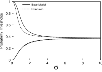
Figure 1:

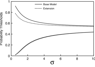
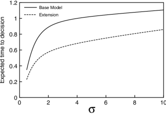
Figure 2:

Online Appendix

Proof of Proposition 1: Statement (i) is proved by Ryan and Lippman (2003) and Kwon et al. (2008). Statement (ii) can be proved similarly.  

Proof of Theorem 1: (i) Consider the following test function:

$$f(p)=\left\{\begin{array}[]{ll}c_{1}\psi(p)+c_{2}\phi(p)&\mbox{if }\>p\in(\underline{\theta},\bar{\theta})\\ g(p)&\mbox{otherwise}\>.\end{array}\right.$$

By Theorem 10.4.1 of Oksendal (2003), the test function $f(p)$ is the optimal return if the following conditions are satisfied: (a) $f(\cdot)$ is continuously differentiable on $[0,1]$, (b) $f(p)\geq g(p)$ for all $p\in[0,1]$, (c) $f(\cdot)$ is twice continuously differentiable except at $\{\underline{\theta},\bar{\theta}\}$, (d) the second-order derivatives of $f(\cdot)$ are finite near $\underline{\theta}$ and $\bar{\theta}$, and (e) $\mathcal{A}f(p)\leq 0$ for $p\in[0,1]\backslash\{\bar{\theta},\underline{\theta}\}$. (Note that $\mathcal{A}f(p)$ is not defined at $p=\bar{\theta}$ or $\underline{\theta}$.) Conditions (c) and (d) can be readily verified from the form of $f(\cdot)$. It remains to show that there exist $c_{1},c_{2},\underline{\theta},$ and $\bar{\theta}$ which satisfy (a), (b), and (e).

(a) The condition that $f(\cdot)$ is continuously differentiable can be expressed as follows:

$$c_{1}\psi(\underline{\theta})+c_{2}\phi(\underline{\theta}) = -\alpha^{-1}[\underline{\theta}h+(1-\underline{\theta})\ell]\,,$$ (16)

$$c_{1}\psi(\bar{\theta})+c_{2}\phi(\bar{\theta}) = \alpha^{-1}[\bar{\theta}h^{\dagger}+(1-\bar{\theta})\ell^{\dagger}]-k\,,$$ (17)

$$c_{1}\psi^{\prime}(\underline{\theta})+c_{2}\phi^{\prime}(\underline{\theta}) = -\alpha^{-1}(h-\ell)\>,$$ (18)

$$c_{1}\psi^{\prime}(\bar{\theta})+c_{2}\phi^{\prime}(\bar{\theta}) = \alpha^{-1}(h^{\dagger}-\ell^{\dagger})\>.$$ (19)

Our strategy is to prove that there always exists a solution $\underline{\theta},\bar{\theta},c_{1}$, and $c_{2}$ that satisfies Eqs. (16)-(19) and the inequality $\underline{\theta}<\bar{\theta}$.

For algebraic convenience, we introduce $\underline{q}\equiv\underline{\theta}/(1-\underline{\theta})$, $\bar{q}\equiv\bar{\theta}/(1-\bar{\theta})$, and $\beta\equiv\bar{q}/\underline{q}$, where $0<\underline{q}\leq\bar{q}<\infty$ and $\beta\in[1,\infty)$. After eliminating $c_{1}$ and $c_{2}$ from Eqs. (16)-(19), we obtain a pair of equations for $\underline{q}$ and $\beta$ as follows:

$$\underline{q} = Q_{1}(\beta)\equiv(\frac{\gamma-1}{\gamma+1})\frac{-\ell-(\ell^{\dagger}-k\alpha)\beta^{-\frac{1}{2}(\gamma+1)}}{h+(h^{\dagger}-k\alpha)\beta^{\frac{1}{2}(1-\gamma)}}\$$ (20)

$$= Q_{2}(\beta)\equiv(\frac{\gamma+1}{\gamma-1})\frac{-\ell-(\ell^{\dagger}-k\alpha)\beta^{\frac{1}{2}(\gamma-1)}}{h+(h^{\dagger}-k\alpha)\beta^{\frac{1}{2}(\gamma+1)}}\;.$$ (21)

We note that $Q_{1}(1)<Q_{2}(1)$ but $\lim_{\beta\rightarrow\infty}Q_{1}(\beta)=(\frac{-\ell}{h})(\frac{\gamma-1}{\gamma+1})>0$ and $\lim_{\beta\rightarrow\infty}Q_{2}(\beta)=0$, so there is always a solution $\beta\in(1,\infty)$ to $Q_{1}(\beta)=Q_{2}(\beta)$; once $\beta$ is determined, $\underline{q}$ is determined by $\underline{q}=Q_{1}(\beta)$.

(b) Note that the fundamental solutions $\psi(\cdot)$ and $\phi(\cdot)$ are monotonically increasing and decreasing respectively, and they are both convex. Hence, if $c_{1}$ and $c_{2}$ have opposite signs, then the test function $f(p)=c_{1}\psi(p)+c_{2}\phi(p)$ in the interval $(\underline{\theta},\bar{\theta})$ must be either monotonically increasing or monotonically decreasing; this contradicts Eqs. (18) and (19) because $h-\ell>0$ and $h^{\dagger}-\ell^{\dagger}>0$. Thus, $c_{1}$ and $c_{2}$ are either both positive or both negative, so $f(\cdot)$ must be either convex or concave because the fundamental solutions $\psi(\cdot)$ and $\phi(\cdot)$ are both convex. However, $f(\cdot)$ cannot be concave because $f^{\prime}(\bar{\theta})>0>f^{\prime}(\underline{\theta})$ by Eqs. (18) and (19). We conclude that $f(\cdot)$ must be convex. It follows that $c_{1}$ and $c_{2}$ are both positive.

From the fact that $g(\cdot)$ is linear except at $\hat{p}$ and that the first derivative of $g(\cdot)$ discontinuously increases at $\hat{p}$, it follows that $\underline{\theta}<\hat{p}<\bar{\theta}$ because otherwise the first derivative of $f(\cdot)$ is constant over the interval $(\underline{\theta},\bar{\theta})$. Moreover, because $f^{\prime\prime}(p)>g^{\prime\prime}(p)$ for all $p\in(\underline{\theta},\bar{\theta})\backslash\{\hat{p}\}$, we have the inequality $f(p)>g(p)$ for $p\in(\underline{\theta},\bar{\theta})$.

(e) Note that $f(\cdot)$ is a strictly positive function. Hence, $g(p)$ is positive for $p\not\in(\underline{\theta},\bar{\theta})$. Because $g(\cdot)$ is linear except at $\hat{p}\in(\underline{\theta},\bar{\theta})$ (piecewise linear), the inequality $\mathcal{A}g(p)=-\alpha g(p)<0$ is satisfied for $p\not\in(\underline{\theta},\bar{\theta})$. Hence, $\mathcal{A}f(p)=0$ for $p\in(\underline{\theta},\bar{\theta})$ and $\mathcal{A}f(p)=\mathcal{A}g(p)<0$ for $p\not\in(\underline{\theta},\bar{\theta})$. This concludes the proof of part (i).

(ii) In order to compute $E^{p}[\tau^{*}]$, we define $\mathcal{L}$, the infinitesimal generator of $P_{t}$, by

$$\mathcal{L}\equiv\frac{1}{2}\frac{(h-\ell)^{2}}{\sigma^{2}}p^{2}(1-p)^{2}\frac{\partial^{2}}{\partial p^{2}}$$

and notice that the probability that $P_{\tau}$ hits the upper threshold first is given by $\mathcal{P}(P_{\tau^{*}}=\bar{\theta})=(p-\underline{\theta})/(\bar{\theta}-\underline{\theta})$ from II.4 and II.9 of Borodin and Salminen (2002). Using the fact that $\mathcal{L}T(p)=1$ and Dynkin’s formula (Oksendal 2003), we obtain

$$E^{p}[\tau^{*}] = E^{p}[\int_{0}^{\tau^{*}}ds]=E^{p}[\int_{0}^{\tau^{*}}\mathcal{L}T(P_{t})dt]$$

$$= E^{p}[T(P_{\tau^{*}})]-T(p)\>,$$

which reduces to Eq. (9).  

Proof of Proposition 2: First, note that the volatility $\frac{h-\ell}{\sigma}P_{t}(1-P_{t})$ of the process $\mathbf{P}=\{P_{t}:t\geq 0\}$ in Eq. (2) is inversely proportional to $\sigma$. Second, note that $R^{*}(p)$ is convex in $p$. Now we can directly apply Theorem 4 of Alvarez (2003) and conclude that $R^{*}(p)$ is non-decreasing in the volatility of $P_{t}$ and hence non-increasing in $\sigma$. Because the continuation region $(\underline{\theta},\bar{\theta})$ is defined as $\{p:R^{*}(p)>g(p)\}$, it follows that $\bar{\theta}$ decreases in $\sigma$ and that $\underline{\theta}$ increases in $\sigma$.  

Proof of Theorem 2: (i) In the small-$\sigma$ limit, we expand Eqs. (20) and (21) in powers of $\sigma$ and study the leading-order terms to obtain the following asymptotic solution to $Q_{1}(\beta)=Q_{2}(\beta)$ where $\beta\equiv\bar{\theta}(1-\underline{\theta})/[\underline{\theta}(1-\bar{\theta})]$ :

$$\beta = \frac{(\ell^{A}-k\alpha)(h^{A}-k\alpha)}{\ell(h^{\dagger}-k\alpha)}\cdot\frac{(h-\ell)^{4}}{4\sigma^{4}\alpha^{2}}+o(\sigma^{-4})\>,$$

$$\underline{\theta} = \frac{-\ell}{h^{A}-k\alpha}\cdot\frac{2\sigma^{2}\alpha}{(h-\ell)^{2}}+o(\sigma^{2})\>,$$

$$\bar{\theta} = 1-\frac{(h^{\dagger}-k\alpha)}{(-\ell^{A}+k\alpha)}\cdot\frac{2\sigma^{2}\alpha}{(h-\ell)}+o(\sigma^{2})\>.$$

Moreover, from $T(p)=\frac{2\sigma^{2}}{(h-\ell)^{2}}(2p-1)\ln\frac{x}{1-x}$, we have $T(\underline{\theta})=-\frac{2\sigma^{2}}{(h-\ell)^{2}}\ln\sigma^{2}+O(\sigma^{2})$ and $T(\bar{\theta})=\frac{2\sigma^{2}}{(h-\ell)^{2}}\ln\frac{1}{\sigma^{2}}+O(\sigma^{2})$, so $E^{p}[\tau^{*}]\rightarrow 0$ as $\sigma\rightarrow 0$.

(ii) and (iii): From

$$g(\hat{p})=\frac{1}{\alpha}\frac{h(\ell^{\dagger}-k\alpha)-\ell(h^{\dagger}-k\alpha)}{h^{A}-\ell^{A}}$$

and $h^{A}-\ell^{A}>0$, the condition $g(\hat{p})\geq 0$ reduces to $h(\ell^{\dagger}-k\alpha)-\ell(h^{\dagger}-k\alpha)\geq 0$ while $g(\hat{p})<0$ reduces to $h(\ell^{\dagger}-k\alpha)-\ell(h^{\dagger}-k\alpha)<0$. From the fact that $\underline{\theta}$ increases and $\bar{\theta}$ decreases in $\sigma$, we find that two alternative cases are possible in the $\sigma\rightarrow\infty$ limit : $\beta\searrow 1$ or $\beta\searrow\beta_{C}>1$.

Assume that $\beta\searrow\beta_{C}>1$. Solving Eqs. (20) and (21) in the large-$\sigma$ limits, we find

$$\beta_{C}=\frac{h(\ell^{\dagger}-k\alpha)}{\ell(h^{\dagger}-k\alpha)}$$

so that $\beta\searrow\beta_{C}>1$ if and only if $h(\ell^{\dagger}-k\alpha)-\ell(h^{\dagger}-k\alpha)<0$ or $g(\hat{p})<0$. In this case, from Eq. (20), we obtain the limiting behaviors $\underline{\theta}\nearrow-\ell/(h-\ell)$ and $\bar{\theta}\searrow-(\ell^{\dagger}-k\alpha)/(h^{\dagger}-\ell^{\dagger})$ as $\sigma\rightarrow\infty$. Moreover, from Eq. (9), it can be shown that $E^{p}[\tau^{*}]\rightarrow\infty$ if $p\in(\frac{-\ell}{h-\ell},\frac{-\ell^{\dagger}+k\alpha}{h^{\dagger}-\ell^{\dagger}})$. On the other hand, if $p\not\in[\frac{-\ell}{h-\ell},\frac{-\ell^{\dagger}+k\alpha}{h^{\dagger}-\ell^{\dagger}}]$, then $E^{p}[\tau^{*}]\rightarrow 0$ because $p$ eventually belongs to the stopping region (the complement of the continuation region) as $\sigma\rightarrow\infty$. Lastly, from Eq. (9) and the fact that $\beta=\beta_{C}+O(\sigma^{-1})$, $\underline{\theta}=\frac{-\ell}{h-\ell}+O(\sigma^{-1})$, and $\bar{\theta}=\frac{-\ell^{\dagger}+k\alpha}{h^{\dagger}-\ell^{\dagger}}+O(\sigma^{-1})$, we obtain $E^{p}[\tau^{*}]=O(\sigma)$ for $p=\frac{-\ell}{h-\ell}$ or $\frac{-\ell^{\dagger}+k\alpha}{h^{\dagger}-\ell^{\dagger}}$.

If $h(\ell^{\dagger}-k\alpha)-\ell(h^{\dagger}-k\alpha)\geq 0$ or $g(\hat{p})\geq 0$, solving Eqs. (20) and (21), we obtain

$$\beta=1+\frac{(h^{A}-k\alpha)(\ell^{A}-k\alpha)}{\ell(h^{\dagger}-k\alpha)-h(\ell^{\dagger}-k\alpha)}\cdot\frac{(h-\ell)^{2}}{2\alpha^{2}\sigma^{2}}+O(\sigma^{-4})\>,$$

$\underline{\theta}=\hat{p}+O(\sigma^{-2})$, and $\bar{\theta}=\hat{p}+O(\sigma^{-2})$ such that $\underline{\theta}\nearrow\hat{p}$, $\bar{\theta}\searrow\hat{p}$ as $\sigma\rightarrow\infty$. Moreover, from Eq. (9), $E^{\hat{p}}[\tau^{*}]=O(\sigma^{-2})$.  

Proof of Theorem 3: We show that (a) the optimal policy exists, (b) there is a component of the continuation region containing $\hat{p}$, and (c) the optimal return function is a continuously differentiable function satisfying Eq. (11).

(a) We closely follow the proof of Proposition 7.1 in Decamps et al. (2005). Upon inspection of the objective function $R_{\tau}(\cdot)$, it is clear that the optimal policy, if it exists, should be stationary because the discounted reward function $e^{-\alpha t}g(p)$ is homogeneous in time. Our objective is to see if there is $\tau^{*}$ such that

$$\bar{R}(p)\equiv\sup_{\tau}R_{\tau}(p)=R^{*}(p)\>.$$

Note that $(t,P_{t})$ is a Feller process and that $e^{-\alpha t}g(p)$ is a continuous and bounded function of $(t,p)$ for $t>0$ and $p\in\Delta$; hence, $\bar{R}(p)$ is bounded and lower semicontinuous (Peskir and Shiryaev 2006, p. 49). It follows that the set $C=\{p:\bar{R}(p)>g(p)\}$ is an open set, and the exit time $\tau_{C}=\inf\{t\geq 0:P_{t}\not\in C\}$ is a well-defined stopping time. From Decamps et al. (2005) p. 497, the stopped process $\{e^{-\alpha(t\wedge\tau_{C})}\bar{R}(P_{t\wedge\tau_{C}}):t\geq 0\}$ is a martingale. Hence, for any positive integer $M$,

$$\bar{R}(p) = E^{p}[e^{-\alpha(M\wedge\tau_{C})}\bar{R}(P_{M\wedge\tau_{C}})]$$

$$= E^{p}[e^{-\alpha\tau_{C}}g(P_{\tau_{C}})\mathbf{1}_{\{\tau_{C}\leq M\}}]+E^{p}[e^{-\alpha M}\bar{R}(P_{M})\mathbf{1}_{\{\tau_{C}>M\}}]\>.$$

The supremum $\bar{R}(p)$ is always non-negative because the return from never stopping is $R_{\infty}(p)=0$ and $R_{\infty}(p)\leq\bar{R}(p)$ by the definition of $\bar{R}(p)$. By the monotone convergence theorem, we have

$$\lim_{M\rightarrow\infty}E^{p}[e^{-\alpha\tau_{C}}g(P_{\tau_{C}})\mathbf{1}_{\{\tau_{C}\leq M\}}]=E^{p}[e^{-\alpha\tau_{C}}g(P_{\tau_{C}})]\>.$$

Also

$$\lim_{M\rightarrow\infty}E^{p}[e^{-\alpha M}\bar{R}(P_{M})\mathbf{1}_{\{\tau_{C}>M\}}]=0\$$

because $\bar{R}(\cdot)$ is bounded. Thus, $\bar{R}(p)=E^{p}[e^{-\alpha\tau_{C}}g(P_{\tau_{C}})]=R^{*}(p)$, so $\tau^{*}=\tau_{C}$: an optimal policy exists.

(b) Because the continuation region is an open set, it suffices to show that the indifference point $\hat{p}$ belongs to the continuation region, which was achieved by Decamps et al. (2006) Proposition 2.2. Hence, there is an interval $(\underline{\theta},\bar{\theta})$ containing $\hat{p}$ which is a component of the continuation region.

(c) Note that $g(\cdot)$ is a bounded and continuous function, and $\mathbf{P}$ is a Markov process. Hence, we can apply Theorem 3.15 of Shiryaev (1978), p. 157 to prove $\mathcal{A}R^{*}(p)=0$ for $p\in C$ and $R^{*}(p)=g(p)$ for $p\notin C$. Thus, for $p\in C$, $R^{*}(p)$ is given by Eq. (11). Moreover, because $\mathbf{P}$ is a diffusive process without any jump, $R^{*}(\cdot)$ is continuous (Peskir and Shiryaev 2006, p. 148) at $\underline{\theta}$ and $\bar{\theta}$. Lastly, because of the regularity of the diffusive process $\mathbf{P}$, the first derivative of $R^{*}(\cdot)$ is continuous at $\underline{\theta}$ and $\bar{\theta}$ (Peskir and Shiryaev 2006, p. 150).  

Proof of Proposition 3: Let $R_{0}^{*}(\cdot)$ and $(\underline{\theta}_{0},\bar{\theta}_{0})$ denote the optimal return function and the continuation region without the post-expansion exit option. [$R_{0}^{*}(\cdot)$ and $(\underline{\theta}_{0},\bar{\theta}_{0})$ are obtained in Sec. 3.] Similarly, let $g_{0}(\cdot)$ denote the gain function defined in Eq. (5). Note that $(\underline{\theta}_{0},\bar{\theta}_{0})=\{p\in(0,1):R_{0}^{*}(p)>g_{0}(p)\}$ and $(\underline{\theta},\bar{\theta})=\{p\in(0,1):R^{*}(p)>g(p)\}$. Because $g(p)\geq g_{0}(p)$ for all $p$, we have $R^{*}(p)\geq R_{0}^{*}(p)$. Moreover, for sufficiently small $p$, $g(p)=g_{0}(p)$.

Suppose that $\underline{\theta}_{0}<\underline{\theta}$. Then $g(\underline{\theta})=g_{0}(\underline{\theta})<R_{0}^{*}(\underline{\theta})$. However, we have $g(\underline{\theta})=R^{*}(\underline{\theta})\geq R_{0}^{*}(\underline{\theta})$, a contradiction. We conclude that $\underline{\theta}_{0}\geq\underline{\theta}$.  

Proof of Lemma 1: The equations for $\underline{\theta}$ and $\bar{\theta}$ can be obtained from the condition that $R^{*}(\cdot)$ is continuously differentiable at $\underline{\theta}$ and $\bar{\theta}$:

$$c_{1}\psi(\underline{\theta})+c_{2}\phi(\underline{\theta}) = -\alpha^{-1}[\underline{\theta}h+(1-\underline{\theta})\ell]\,,$$

$$c_{1}\psi(\bar{\theta})+c_{2}\phi(\bar{\theta}) = V^{A}(\bar{\theta})-k-\alpha^{-1}[\bar{\theta}h+(1-\bar{\theta})\ell]\,,$$

$$c_{1}\psi^{\prime}(\underline{\theta})+c_{2}\phi^{\prime}(\underline{\theta}) = -\alpha^{-1}(h-\ell)\>,$$

$$c_{1}\psi^{\prime}(\bar{\theta})+c_{2}\phi^{\prime}(\bar{\theta}) = V^{A\prime}(\bar{\theta})-\alpha^{-1}(h-\ell)\>.$$

After eliminating $c_{1}$ and $c_{2}$, using the form of $V^{A}(p)$ when $V^{A}(p)>k$, we obtain the following equations in terms of $\underline{q}\equiv\underline{\theta}/(1-\underline{\theta})$, $\bar{q}\equiv\bar{\theta}/(1-\bar{\theta})$, and $\beta\equiv\bar{q}/\underline{q}$:

$$\underline{q} = (\frac{\gamma-1}{\gamma+1})\frac{-\ell-(\ell^{\dagger}-k\alpha)\beta^{-\frac{1}{2}(\gamma+1)}}{h+(h^{\dagger}-k\alpha)\beta^{\frac{1}{2}(1-\gamma)}}\$$ (22)

$$= (\frac{\gamma+1}{\gamma-1})\frac{-\ell-(\ell^{\dagger}-k\alpha)\beta^{\frac{1}{2}(\gamma-1)}}{h+(h^{\dagger}-k\alpha)\beta^{\frac{1}{2}(\gamma+1)}}-\frac{2\alpha C\gamma}{\gamma-1}\frac{\underline{q}^{-\frac{1}{2}(\gamma-1)}}{h+(h^{\dagger}-k\alpha)\beta^{\frac{1}{2}(\gamma+1)}}$$ (23)

From Eqs. (22), (23), and (10), we obtain Eqs. (12) and (13).  

Proof of Proposition 4: From $\ell^{A}<0$, we have $1-\sigma^{2}\frac{2(h^{\dagger}-k\alpha)}{k(h-\ell)^{2}}<1-\sigma^{2}\frac{2(h^{\dagger}-k\alpha)}{(k-\ell^{A}/\alpha)(h-\ell)^{2}}$, so $\bar{\theta}$ is smaller with the post-expansion exit option. It follows that the expected time-to-decision is also smaller up to $o(\sigma^{2})$.  

Proof of Proposition 5: Let $\beta_{\infty}$ denote $\lim_{\sigma\rightarrow\infty}\beta$. Then we consider two cases: $\beta_{\infty}>1$ and $\beta_{\infty}=1$.

(i) $\beta_{\infty}>1$: From Eq. (22), the second term of Eq. (23) is

$$-4\frac{\sqrt{h^{A}\ell^{A}\ell/(h\beta_{\infty})}}{e\gamma(h^{\dagger}-k\alpha)}(\frac{\ell^{A}h}{\ell h^{A}\beta_{\infty}})^{\gamma/2}(1+o(1))\>.$$

For Example 1, $h^{A}/|\ell^{A}|=h/|\ell|$, so $\frac{\ell^{A}h}{\ell h^{A}\beta_{\infty}}<1$. For Example 2, $h^{A}>h$ and $|\ell|>|\ell^{A}|$, so again $\frac{\ell^{A}h}{\ell h^{A}\beta_{\infty}}<1$. It follows that $(\frac{\ell^{A}h}{\ell h^{A}\beta_{\infty}})^{\gamma/2}$ converges to zero faster than $\sigma^{-n}$ for any positive $n$. Thus, Eqs. (22) and (23) coincide with (20) and (21) in the large-$\sigma$ limit.

(ii) $\beta_{\infty}=1$: The only possible solution for $\beta$ is of the form $1+O(\sigma^{-2})$. (There is no term of order $O(\sigma^{-1})$.) The second term of Eq. (23) is

$$-\frac{4}{e\gamma}\sqrt{\frac{h^{A}\ell^{A}(\ell^{A}-k\alpha)}{(h^{A}-k\alpha)^{3}}}[\frac{(h^{A}-k\alpha)(-\ell^{A})}{h^{A}(-\ell^{A}+k\alpha)}]^{\gamma/2}(1+o(1))\>.$$

(The factor of $e^{-1}$ comes from the factor $\lim_{\sigma\rightarrow}(\frac{\gamma-1}{\gamma+1})^{\gamma/2}$ in the definition of $C$.) From the fact that $\frac{(h^{A}-k\alpha)(-\ell^{A})}{h^{A}(-\ell^{A}+k\alpha)}<1$, this term converges to zero faster than $\sigma^{-n}$ for any positive $n$. Thus, Eqs. (22) and (23) coincide with (20) and (21) in the large-$\sigma$ limit.

References

- Alvarez (2001) Alvarez, L. H. R. 2001. Reward functionals, salvage values and optimal stopping. Mathematical Methods of Operations Research 54 315–337.
- Alvarez (2003) Alvarez, L. H. R. 2003. On the properties of r-excessive mappings for a class of diffusions. Annals of Applied Probability 13 1517–1533.
- Alvarez and Stenbacka (2004) Alvarez, L. H. R., R. Stenbacka. 2004. Optimal risk adoption: a real options approach. Economic Theory 23(1) 123–147.
- Arrow (1962) Arrow, K. J. 1962. The economic implications of learning by doing. The Review of Economic Studies 29(3) 155–173.
- Bergemann and Välimäki (2000) Bergemann, D., J. Välimäki. 2000. Experimentation in markets. The Review of Economic Studies 67(2) 213–234.
- Bernardo and Chowdhry (2002) Bernardo, A. E., B. Chowdhry. 2002. Resources, real options, and corporate strategy. Journal of Financial Economics 63(2) 211–234.
- Bolton and Harris (1999) Bolton, P., C. Harris. 1999. Strategic experimentation. Econometrica 67(2) 349–374.
- Borodin and Salminen (2002) Borodin, A. N., P. Salminen. 2002. Handbook of Brownian Motion – Facts and Formulae. Birkhauser, Basel, 2nd ed.
- Dayanik and Karatzas (2003) Dayanik, S., I. Karatzas. 2003. On the optimal stopping problem for one-dimensional diffusions. Stochastic Processes and their Applications 107 173–212.
- Decamps et al. (2005) Decamps, J.-P., T. Mariotti, S. Villeneuve. 2005. Investment timing under incomplete information. Mathematics of Operations Research 30(2) 472–500.
- Decamps et al. (2006) Decamps, J.-P., T. Mariotti, S. Villeneuve. 2006. Irreversible investment in alternative projects. Economic Theory 28(2) 425–448.
- Dixit (1989) Dixit, A. 1989. Entry and exit decisions under uncertainty. The Journal of Political Economy 97(3) 620–638.
- Dixit (1992) Dixit, A. 1992. Investment and hysteresis. The Journal of Economic Perspectives 6(1) 107–132.
- Ghemawat and Stander (1998) Ghemawat, P., H. Stander. 1998. Nucor at a crossroads. Harvard Business School Case 9–793–039.
- Hu and Oksendal (1998) Hu, Y., B. Oksendal. 1998. Optimal time to invest when the price processes are geometric brownian motions. Finance and Stochastics 2(3) 295–310.
- Keller and Rady (1999) Keller, G., S. Rady. 1999. Optimal experimentation in a changing environment. The Review of Economic Studies 66(3) 475–507.
- Kwon (2010) Kwon, H. D. 2010. Invest or Exit? Optimal Decisions in the Face of a Declining Profit Stream. Operations Research 58(3) 638–649.
- Kwon et al. (2008) Kwon, H. D., S. A. Lippman, C. S. Tang. 2008. When to adjust price under incomplete information. UCLA Working Paper.
- Lai (2001) Lai, T. L. 2001. Sequential analysis: Some classical problems and new challenges. Statistica Sinica 11 303–408.
- Lippman and Rumelt (1992) Lippman, S. A., R. P. Rumelt. 1992. Demand uncertainty, capital specificity, and industry evolution. Ind Corp Change 1(1) 235–262.
- McCardle (1985) McCardle, K. F. 1985. Information acquisition and the adoption of new technology. Management Science 31(11) 1372–1389.
- Moscarini and Smith (2001) Moscarini, G., L. Smith. 2001. The optimal level of experimentation. Econometrica 69(6) 1629–1644.
- Muthuraman and Kumar (2008) Muthuraman, K., S. Kumar. 2008. Solving free-boundary problems with applications in finance. Foundations and Trends in Stochastic Systems 1(4) 259–341.
- Oksendal (2003) Oksendal, B. 2003. Stochastic Differential Equations: An Introduction with Applications. Springer, 6th ed.
- Olsen and Stensland (1992) Olsen, T. E., G. Stensland. 1992. On optimal timing of investment when cost components are additive and follow geometric diffusions. Journal of Economic Dynamics and Control 16(1) 39–51.
- Peskir and Shiryaev (2006) Peskir, G., A. Shiryaev. 2006. Optimal Stopping and Free-Boundary Problems. Birkhauser Basel.
- Poor and Hadjiliadis (2008) Poor, H. V., O. Hadjiliadis. 2008. Quickest Detection. Cambridge University Press.
- Ryan and Lippman (2003) Ryan, R., S. A. Lippman. 2003. Optimal exit from a project with noisy returns. Probab. Engrg. Inform. Sci. 17(04) 435–458.
- Shiryaev (1978) Shiryaev, A. 1978. Optimal Stopping Rules. Springer-Verlag, New York.
- Shiryaev (1967) Shiryaev, A. N. 1967. Two problems of sequential analysis. Cybernetics and Systems Analysis 3(2) 63–69.
- Ulu and Smith (2009) Ulu, C., J. E. Smith. 2009. Uncertainty, Information Acquisition, and Technology Adoption. Operations Research 57(3) 740–752.
- Wald (1945) Wald, A. 1945. Sequential tests of statistical hypotheses. Annals of Mathematical Statistics 16 117–186.
- Wald (1973) Wald, A. 1973. Sequential Analysis. Dover Publications.
- Wang (2005) Wang, H. 2005. A sequential entry problem with forced exits. Mathematics of Operations Research 30 501–520.