Dimension Theory of some non-Markovian repellers Part I: A gentle introduction

Abstract.

Michael Barnsley introduced a family of fractals sets which are repellers of piecewise affine systems. The study of these fractals was motivated by certain problems that arose in fractal image compression but the results we obtained can be applied for the computation of the Hausdorff dimension of the graph of some functions, like generalized Takagi functions and fractal interpolation functions.

In this paper we introduce this class of fractals and present the tools in the one-dimensional dynamics and nonconformal fractal theory that are needed to investigate them. This is the first part in a series of two papers. In the continuation there will be more proofs and we apply the tools introduced here to study some fractal function graphs.

1. Introduction

This is a paper in the intersection of fractal geometry and dynamical systems. Dynamical systems provide us with beautiful and interesting examples of sets, fractal geometry gives us the language to describe them, and both theories give us tools. Tools to understand the geometric properties of those sets, tools to understand the dynamical properties, and most interesting of all – the relations between the two.

This is a paper about tools. Yeah, sure, we will prove some theorem eventually (in the second part of this paper) – but it is just a pretext. Our real goal is to describe the process of understanding the geometric behaviour of a dynamical system, starting from understanding the simplest possible models (conformal uniformly hyperbolic iterated function systems with separation properties) and then throwing out the training wheels, until we get to piecewise affine maps with quite general symbolic description (not necessarily subshifts of finite type).

And, most of all, this is a survey. While the simple models are in the books (the classical positions by Falconer [7] and by Mattila [17]), the modern theory of affine iterated function systems is not in books yet, and neither is Hofbauer’s theory. We aren’t going to be able to describe all the details, for sure, but we try to at least provide the main ideas and most useful formulas, and also the literature for further reading.

Fine, let’s present the hero of our story.

2. Barnsley’s skew product maps

In order to define a piecewise affine and piecewise expanding skew product map $F$ on the plane which sends the vertical stripe $D:=[0,1]\times\mathbb{R}$ into itself, first we partition the unit interval ${[0,1]=\bigsqcup\limits_{i=1}^{m}I_{i}}$. Then we define $F:D\to D$ by

(2.1) $$F(x,y):=F_{i}(x,y)\mbox{ if }(x,y)\in{D_{i}:=I_{i}\times\mathbb{R}},$$

where for all $i=1,\dots,m$

(2.2) $$F_{i}(x,y):=({f_{i}(x)},{g_{i}(x,y)}),\ \mbox{ for }(x,y)\in D_{i}$$

and $f_{i}:I_{i}\to J_{i}\subset[0,1]$ (see Figure 1) and $g_{i}:D_{i}\to\mathbb{R}$ and for $|\lambda_{i}|,|\gamma_{i}|>1$ let

(2.3) $$f_{i}(x):=\gamma_{i}x+v_{i},\ g_{i}(x,y)=a_{i}x+\lambda_{i}y+t_{i}.$$

Throughout this note we always assume:
Principal assumption The map $f:[0,1]\to[0,1]$

(2.4) $$f(x):=f_{i}(x),\mbox{ if }x\in I_{i}\quad\mbox{ is transitive,}$$

that is $f$ has an orbit which is dense in $[0,1]$. We call the repeller of $F:D\to D$ (which is the graph of a function) Barnsley repeller and we denote it by $\Lambda$. We call $F$ Barnsley’s skew product map. Let $\mathfrak{S}=\bigcup_{i=1}^{M}\partial I_{i}$ the singularity set and let $\mathfrak{S}_{\infty}=\bigcup_{n=0}^{\infty}f^{-n}(\mathfrak{S})$. It was pointed out by Barnsley that $\Lambda$ is the graph of a function $G:[0,1]\setminus\mathfrak{S}_{\infty}:\to\mathbb{R}$ which is defined by

(2.5) $$G(x)=z\text{, where }\{F^{n}(x,z)\}_{n=1}^{\infty}\text{ is bounded.}$$

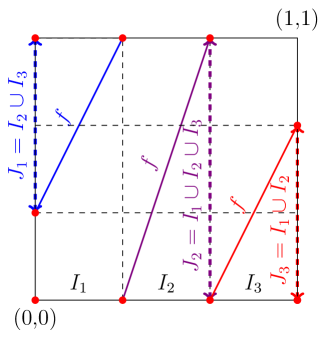
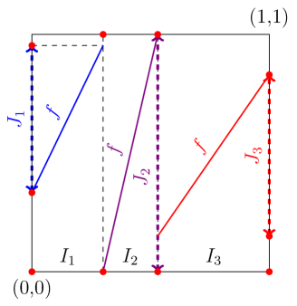
Figure 1. $f$ is Markov on the left hand-side and non-Markov on the righ-hand side.

3. The Hausdorff and box dimensions

For a $d\geq 1$ let $A\subset\mathbb{R}^{d}$ be a set of zero Lebesgue measure and let $\nu$ be a measure which is singular with respect to the Lebesgue measure $\mathcal{L}_{d}$. Then the size of $A$ and $\nu$ can be expressed by their fractal dimensions.

3.1. Fractal dimensions of sets

The most common fractal dimensions are the Hausdorff and the box dimensions:

Definition 3.1 (Hausdorff dimension).

Let $A\subset\mathbb{R}^{d}$. then

(3.1) $$\dim_{\rm H}A:=\inf\left\{\alpha:\forall\varepsilon>0,\exists\left\{U_{i}\right\}_{i=1}^{\infty},\mbox{ such that }A\subset\bigcup\limits_{i=1}^{\infty}U_{i},\ \sum\limits_{i=1}^{\infty}|U_{i}|^{\alpha}<\varepsilon\right\},$$

where $|U_{i}|$ is the diameter of $U$.

Equivalently in a more traditional way we can first define the $t$-dimensional Hausdorff measure

(3.2) $$\mathcal{H}^{t}(A)=\sup\limits_{\delta\to 0}\inf\left\{\boxed{\sum\limits_{i=1}^{\infty}|E_{i}|^{t}}:\Lambda\subset\bigcup_{i=1}^{\infty}E_{i},|E_{i}|<\delta\right\},$$

then we write see (Figure 3.1)

(3.3) $$\dim_{\rm H}A:=\inf\left\{t:\mathcal{H}^{t}(A)=0\right\}=\sup\left\{t:\mathcal{H}^{t}(A)=\infty\right\}.$$

Another very popular notion of fractal dimension is the box dimension:

Definition 3.2.

$\dim_{\rm B}A$

Let $E\subset\mathbb{R}^{d}$, $E\neq\emptyset$, bounded. $N_{\delta}(E)$ be the smallest number of sets of diameter $\delta$ which can cover $E$. Then the lower and upper box dimensions of $E$:

(3.4) $$\underline{\dim}_{\rm B}(E):=\liminf_{r\to 0}\frac{\log N_{\delta}(E)}{-\log\delta},$$

(3.5) $$\overline{\dim}_{\rm B}(E):=\limsup_{r\to 0}\frac{\log N_{\delta}(E)}{-\log\delta}.$$

If the limit exists then we call it the box dimension of $E$ and we denote it by $\dim_{\rm B}(E)$.

3.2. Hausdorff dimension of measures

The Hausdorff dimension of a measure $\mu$ is the best lower bound on the Hausdorff dimension of a sets having large $\mu$ measures. Depending on what ”large” means we define

Definition 3.3.

Let $\mu$ be a Borel measure on $\mathbb{R}^{d}$ such that $0<\mu(\mathbb{R}^{d})<\infty$.

(a):

Lower Hausdorff dimension of $\mu$ is: $\mathrm{dim}_{*}(\mu):=\inf\left\{\dim_{\rm H}A:\mu(A)>0\right\}$,

(b):

Upper Hausdorff dimension of $\mu$: $\mathrm{dim}^{*}(\mu):=\inf\left\{\dim_{\rm H}A:\mu(A^{c})=0\right\}$.

(c):

The lower and the upper local dimension of the measure $\mu$ are:

(3.6) $${\underline{\dim}(\mu,x):=\liminf\limits_{r\to 0}\frac{\log\mu(B(x,r))}{\log r}}$$

and

(3.7) $${\overline{\dim}(\mu,x):=\limsup\limits_{r\to 0}\frac{\log\mu(B(x,r))}{\log r}}$$

We say that the measure $\mu$ is exact dimensional if for $\mu$-almost all $x$ $\lim\limits_{r\downarrow 0}\frac{\log\mu(B(x,r))}{\log r}$ exists and equals to a constant.

Lemma 3.4.

Let $\mu$ be a measure like in (3.3). Then

(3.8) $${\dim_{*}\mu=\mathrm{essinf}_{x\sim\mu}\underline{\dim}(\mu,x)},\quad{\dim^{*}\mu=\mathrm{esssup}_{x\sim\mu}\underline{\dim}(\mu,x)}$$

4. Self-similar Sets

From now on we work on $\mathbb{R}^{d}$. Let $m\geq 2$ and $O_{1},\dots,O_{m}\in O(d)$ orthogonal matrices and $r_{1},\dots,r_{m}\in(0,1)$ and $t_{1},\dots,t_{m}\in\mathbb{R}^{d}$. Then

(4.1) $${\mathcal{S}:=\left\{S_{i}(x)=r_{i}\cdot O_{i}x+t_{i}\right\}_{i=1}^{m}}$$

is called a self-similar Iterated Function System on $\mathbb{R}^{d}$.

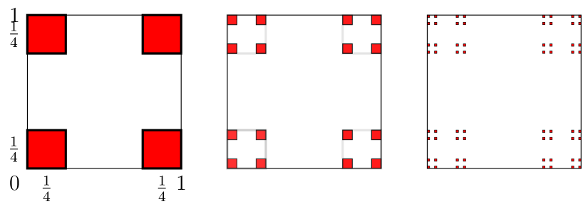
Figure 2. The Four-Corner Cantor set $C\left(\frac{1}{4}\right)$

Let $B:=B(x,R)$ be a closed ball, where $R$ is large. Then

(4.2) $$\forall i=1,\dots,m:\quad{S_{i}(B)\subset B}.$$

Hence the the following is a nested sequence of compact sets:

$$\left\{{\bigcup_{i_{1}\dots i_{n}}S_{i_{1}\dots i_{n}}B}\right\}_{n=1}^{\infty},$$

where we use throughout the paper the notation: $S_{i_{1}\dots i_{n}}:=S_{i_{1}}\circ\cdots\circ S_{i_{n}}$. The attractor of our IFS $\mathcal{S}$ is

(4.3) $${{\Lambda}:=\bigcap_{n=1}^{\infty}\bigcup_{i_{1}\dots i_{n}}S_{i_{1}\dots i_{n}}B},$$

which is independent of $B$ as long as $B$ satisfies (4.2).

Example 4.1 (Four Corner Set).

Figure 2 shows the first three iterations of a famous self-similar set, called the Four Corner Cantor set. Here $B=[0,1]^{2}$ and

$$S_{i}(x,y)=\frac{1}{4}(x,y)+\mathbf{t}_{i},\mbox{ for }\mathbf{t}_{1}=(0,0),\ \mathbf{t}_{2}=\left(\frac{3}{4},0\right),\mathbf{t}_{3}=\left(\frac{3}{4},\frac{3}{4}\right),\mathbf{t}_{3}=\left(0,\frac{3}{4}\right).$$

In the general case, we code the points of the attractor by the elements of the symbolic space:

(4.4) $$\Sigma:=\left\{1,\dots,m\right\}^{\mathbb{N}}.$$

The natural projection is $\Pi:\Sigma\to\Lambda$:

(4.5) $${\Pi(\mathbf{i}):=\lim\limits_{n\to\infty}S_{i_{1}\dots i_{n}}(0).}$$

On Figures 3 and 4 we indicate how this coding works.

Figure 3. the Sierpiński gasket: $S_{312}(x):=S_{3}\circ S_{1}\circ S_{2}(x)=S_{3}(S_{1}(S_{2}(x)))$

$S_{i}$ are translations of the appropriate homothety-transformatons of the form:

$${S_{i}(x)=\frac{1}{2}x+t_{i}}.$$

The sets $\left\{S_{i}(T)\right\}_{i=1}^{3}$ in the previous examples ar the first cylinders, the sets $\left\{S_{i,j}(T)\right\}_{i,j=1}^{3}$ are the second cylinders an so on.

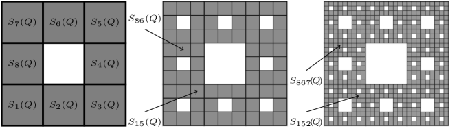
Figure 4. The third approximation of the Sierpiński carpet

In both of the previous examples the cylinders were not disjoint but their interior were disjoint. This results that the cylinders are well separated.

Definition 4.2 ( SSP,OSC,SOSC).

Here we define three important separation conditions. These will be used in much more general setup then the self-similar IFS.

(a):

If $S_{i}(\Lambda)\cap S_{j}(\Lambda)=\emptyset$ for all $i\neq j$ the we say that the Strong Separation Property (SSP) holds. (Like in the case of the Four Corner Cantor set.)

(b):

If there exists a bounded open set $V$ such that

1. $S_{i}(V)\subset V$ for all $i=1,\dots,m$

2. $S_{i}(V)\cap S_{j}(V)=\emptyset$ for all $i\neq j$ then we say that the Open Set Condition (OSC) holds like in the case of the Sierpiński gasket and Sierpiński carpet. Here $V$ is the interior of the right triangle and the unit square respectively.

3. If the OSC holds with an open set $V$ satisfying $V\cap\Lambda\neq\emptyset$, where $\Lambda$ is the attractor, then we say that the Strong Open Set Condition (SOSC) holds.

The OSC and SOSC are equivalent for self-similar (and also for self-conformal) IFS.

Now we present a heuristic argument in order to guess the Hausdorff dimension of the attractor $\Lambda$ in the case when the cylinders are disjoint (that is when SSP holds):

We will use the following fact: it is immediate from the definition that for any $r>0$ we have:

(4.6) $${\mathcal{H}^{s}(r\cdot A):=r^{s}\cdot\mathcal{H}^{s}(A)}.$$

Since this is only a heuristic argument we assume that for the appropriate $s$, (that is for the $s$ satisfying $s=\dim_{\rm H}\Lambda$) the $s$-dimensional Hausdorff measure of the attractor $\Lambda$ has positive and finite. Then

$${\mathcal{H}^{s}(\Lambda)} = \sum\limits_{i=1}^{m}\mathcal{H}^{s}(S_{i}\Lambda)$$

$$= \sum\limits_{i=1}^{m}r_{i}^{s}{\mathcal{H}^{s}(\Lambda)}.$$

By the assumption above, we can divide by $\mathcal{H}^{s}(\Lambda)$. This yields that:

(4.7) $${\sum\limits_{i=1}^{m}r_{i}^{{s}}=1.}$$

Even if $\mathcal{S}$ does not satisfy any of the previous assumptions we can define $s$ as the solution of (4.7).

Definition 4.3.

Let $\mathcal{S}$ be a self-similar IFS of the form (4.1). The similarity dimension $\dim_{\rm S}(\Lambda):=s$ where $s$ is the unique solution of (4.7). That is ${\sum\limits_{i=1}^{m}r_{i}^{{s}}=1}.$ Sometimes we also say that $s$ is the similarity dimension of the attractor.

Clearly,

(4.8) $${\dim_{\rm H}(\Lambda)\leq\dim_{\rm S}(\Lambda)}.$$

However ”$=$” does not always hold:

Let $\Lambda_{1/3}$ be the attractor the $\mathcal{S}^{1/3}$ from (4.11):

$${\mathcal{S}^{1/3}=\mathcal{S}:=\left\{\frac{1}{3}x,\frac{1}{3}x+1,\frac{1}{3}x+3\right\}}.$$

Then

(4.9) $$\dim_{\rm B}(\Lambda_{1/3})<0.9<1=\dim_{\rm S}(\Lambda_{1/3}).$$

This is so because in this case

$$S^{1/3}_{0}\circ S^{1/3}_{3}\equiv S^{1/3}_{1}\circ S^{1/3}_{0}$$

so there is an exact overlap.

Theorem 4.4 (Hutchinson’s-Moran Theorem [18] and [13]).

Let $\mathcal{S}:=\left\{S_{1},\dots,S_{m}\right\}$ be a self-similar IFS on $\mathbb{R}^{d}$ with contraction ratios $r_{1},\dots,r_{m}$ and similarity dimension $s$. We assume that the OSC (Open Set Condition) holds.

then

(a):

${\dim_{\rm H}\Lambda=s}$, even we have

(b):

$0<\mathcal{H}^{s}(\Lambda)<\infty$,

(c):

$\mathcal{H}^{s}\left(S_{i}(\Lambda)\cap S_{j}(\Lambda)\right)=0$ for all $i\neq j$.

Theorem 4.5 (Falconer).

The Hausdorff- and box-dimensions are the same for any self-similar set.

The following problem is one of the most interesting open problems in Fractal Geometry:

Conjecture 4.6 (Complete Overlap Conjecture).

Let $s$ be the similarity dimension and let $\Lambda$ be the attractor of a self-similar IFS $\mathcal{S}=\left\{S_{i}\right\}_{i=1}^{m}$ on $\mathbb{R}$. Then

(4.10) $${\dim_{\rm H}(\Lambda)<\min\left\{d,s\right\}}\Longleftrightarrow\exists\mathbf{i},\ \mathbf{j}\in\Sigma^{*},\mathbf{i}\neq\mathbf{j}\mbox{ s.t. }{S_{\mathbf{i}}\equiv S_{\mathbf{j}}}.$$

In $\mathbb{R}^{2}$ the conjecture does not hold. The following example was introduced by M. Keane, M. Smorodinsky and B. Solomyak [15] and played a very important role in the study of self-similar fractals with overlapping construction.

Example 4.7.

For every $\lambda\in(\frac{1}{4},\frac{2}{5})$ consider the following self-similar set:

$${{\widetilde{\Lambda}_{\lambda}}:=\left\{{\sum\limits_{i=0}^{\infty}a_{i}\lambda^{i}}:a_{i}\in\left\{0,1,3\right\}\right\}.}$$

Then ${\widetilde{\Lambda}_{\lambda}}$ is the attractor of the one-parameter ($\lambda$) family IFS:

(4.11) $${\mathcal{S}^{\lambda}:=\left\{{S_{i}^{\lambda}(x)}:=\lambda\cdot x+i\right\}_{i=0,1,3}}$$

To normalize it we write $\Lambda_{\lambda}:=\frac{1-\lambda}{3}\cdot\widetilde{\Lambda}_{\lambda}$. It was proved by Solomyak [21] that for Lebesgue almost all $\lambda>\frac{1}{3}$ (that is when the similarity dimension is greater than one) we have

(4.12) $$\dim_{\rm H}\Lambda_{\lambda}=1.$$

Fix a $\lambda$ slightly greater than $1/3$ for which (4.12) holds and consider the product set $C_{\lambda}:=\Lambda_{\lambda}\times[0,1]$ (see Figure 5). Then for $\lambda\in\left(\frac{1}{3},\frac{1}{\sqrt{6}}\right)$we have

$$\dim_{\rm H}C_{\lambda}=1+\frac{\log 2}{-\log\lambda}<\min\left\{2,\frac{\log 6}{-\log\lambda}\right\}=\min\left\{2,\dim_{\rm Sim}(\mathcal{S})\right\}.$$

Since there are uncountably many $\lambda$ like this, and complete overlap can happen only for countably many $\lambda$, we get that dimension drop occur in higher dimension not only when we have complete overlaps.

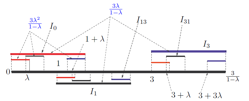
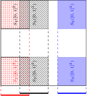
Figure 5. $\widetilde{\Lambda}_{\lambda}$ and $C_{\lambda}:=\Lambda_{\lambda}\times[0,1]$

4.1. Self-similar measures

Analogously to the self-similar sets, we can define the self-similar measures:

Definition 4.8.

Given an $m\geq 2$, ${\mathcal{S}=\left\{S_{1},\dots,S_{m}\right\}}$ self-similar IFS on $\mathbb{R}^{d}$ with contraction ratios: ${r_{1},\dots,r_{m}}$ and we are given a probability vector ${\mathbf{p}=\left(p_{1},\dots,p_{m}\right)}$. Now we define the self-similar measure $\nu=\nu_{\mathcal{S},\mathbf{p}}$ which corresponds to $\mathcal{S}$ and $\mathbf{p}$:

(4.13) $${\nu_{\mathcal{S},\mathbf{p}}:=\Pi_{*}\left(\mathbf{p}^{\mathbb{N}}\right):=\mu\circ\Pi^{-1}}.$$

Then $\nu_{\mathcal{S},\mathbf{p}}$ is the unique probability Borel measure satisfying

(4.14) $$\nu_{\mathcal{S},\mathbf{p}}(H)=\sum\limits_{k=1}^{m}p_{i}\cdot\nu_{\mathcal{S},\mathbf{p}}\left(S_{i}^{-1}(H)\right),$$

for every Borel set $H$.

Let ${\nu:=\nu_{\mathcal{S},\mathbf{p}}}$ be the invariant measure for the self-similar IFS on $\mathbb{R}^{d}$:

(4.15) $${\mathcal{S}:=\left\{S_{i}(x)=r_{i}\cdot O_{i}x+t_{i}\right\}_{i=1}^{m}}.$$

Below we give a heuristic argument to show that if the OSC holds then the Hausdorff dimension of $\nu$ is equal to the similarity dimension of $\nu$, which is defined by:

(4.16) $${\dim_{\rm{Sim}}\nu:=\frac{\sum\limits_{i=1}^{m}p_{i}\log p_{i}}{\sum\limits_{i=1}^{m}p_{i}\log r_{i}}=\frac{\mbox{entropy}}{\mbox{Lyapunov exponent}}.}$$

Lemma 4.9.

$\mathcal{S}$ and $\mathbf{p}$ as above and we assume that the OSC holds. Then

(4.17) $$\dim_{\rm H}\nu=\dim_{\rm Sim}\nu.$$

Heuristic Proof.

Let $I$ be a large interval such that $S_{i}(I)\subset I$ for all $i=1,\dots,m$ and we write $I_{i_{1}\dots i_{n}}:=S_{i_{1}\dots i_{n}}I$ for the level $n$ cylinder intervals. It follows from Birkhoff’s Ergodic Theorem that in this case the limit in (3.6) and (3.7) exist. That is, Lemma 3.4 indicates that for a $\nu$-typical $x=\Pi(\mathbf{i})$, $\mathbf{i}\in\Sigma$:

$${\dim_{\rm H}\nu} = \lim\limits_{n\to\infty}\frac{\log\nu(I_{i_{1}\dots i_{n}})}{\log|I_{i_{1}\dots i_{n}}|}\stackrel{{\scriptstyle\mathrm{def}}}{{=}}\lim\limits_{n\to\infty}\frac{\log p_{i_{1}\dots i_{n}}}{\log r_{i_{1}\dots i_{n}}}$$

$$= \frac{\lim\limits_{n\to\infty}\frac{1}{n}\sum\limits_{k=1}^{n}\log p_{i_{k}}}{\lim\limits_{n\to\infty}\frac{1}{n}\sum\limits_{k=1}^{n}\log r_{i_{k}}}\stackrel{{\scriptstyle\mathrm{LLN}}}{{=}}{\frac{\sum\limits_{i=1}^{m}p_{i}\log p_{i}}{\sum\limits_{i=1}^{m}p_{i}\log r_{i}}}=\dim_{\rm{Sim}}\nu,$$

where LLN means Law of Large Numbers. Here we used the notations: $p_{i_{1}\dots i_{n}}:=p_{i_{1}}\cdots p_{i_{n}}$ and $r_{i_{1}\dots i_{n}}:=r_{i_{1}}\cdots r_{i_{n}}$ ∎

4.1.1. Hochman Theorem

Let $\mathcal{S}=\left\{S_{i}\right\}_{i=1}^{m}$ be a self-similar IFS on $\mathbb{R}$ with contraction ratios $\left\{r_{i}\right\}_{i=1}^{m}$. Let $\Delta_{n}(\mathcal{S})$ be the smallest distance between the left end points of two level $n$ cylinders having the same length. More formally, $\Delta_{n}(\mathcal{S})$ is the minimum of $\Delta(\boldsymbol{\omega},\boldsymbol{\tau})$ for distinct $\boldsymbol{\omega},\boldsymbol{\tau}\in\Sigma_{n}$, where

$$\Delta(\boldsymbol{\omega},\boldsymbol{\tau})=\left\{\begin{array}[]{cc}\infty&S_{\boldsymbol{\omega}}^{\prime}(0)\neq S_{\boldsymbol{\tau}}^{\prime}(0)\\ \left|S_{\boldsymbol{\omega}}(0)-S_{\boldsymbol{\tau}}(0)\right|&S_{\boldsymbol{\omega}}^{\prime}(0)=S_{\boldsymbol{\tau}}^{\prime}(0).\end{array}\right.$$

Condition 4.10 (HESC).

We say that the self-similar IFS $\mathcal{S}$ satisfies Hochman’s exponential separation condition (HESC) if there exists an $\varepsilon>0$ and an $n_{k}\uparrow\infty$ such that

(4.18) $$\Delta_{n_{k}}>\varepsilon^{n_{k}}.$$

Hochman proved the following very important assertion in [9, Theorem 1.1].

Theorem 4.11 (Hochman).

Assume that $\mathcal{S}=\left\{S_{i}\right\}_{i=1}^{m}$ is a self-similar IFS on $\mathbb{R}$ which satisfies Hochman’s exponential separation condition. Let $\mathbf{p}=(p_{1},\dots,p_{N})$ be an arbitrary probability vector. Then

(4.19) $$\dim_{H}\left(\nu_{\mathcal{S},\mathbf{p}}\right)=\min\left\{1,\dim_{\rm Sim}\nu\right\},$$

Remark 4.12 (Relation to the Compete Overlaps Conjecture).

Although Hochman’s Theorem does not solve the Compete Overlaps Conjecture (Conjecture 4.6) but it makes a very significant progress towards it.

• Exact overlap means that $\Delta_{n}=0$ for some $n$.

• If the OSC holds then ${\Delta_{n}\to 0}$ exactly exponentially fast.

• $\Delta_{n}\to 0$ at least exponentially fast always holds. Namely: ${\#\left\{|\mathbf{i}|=n\right\}=m^{n}}$. On the other hand: $\#\left\{r_{\mathbf{i}}:|\mathbf{i}|=n\right\}$ is polynomially large ($r_{\mathbf{i}}$ was the contraction ration of $S_{\mathbf{i}}$). So, there exist distinct $\mathbf{i},\mathbf{j}$ of length $n$ with $r_{\mathbf{i}}=r_{\mathbf{j}}$ and with with exponentially small ${\left|S_{\mathbf{i}}(0)-S_{\mathbf{j}}(0)\right|}$.

• However, in case of a dimension drop, that is if we can find a probability vector $\mathbf{p}$ such that $\dim_{\rm H}\nu_{\mathcal{S},\mathbf{p}}<\min\left\{1,\dim_{\rm S}\nu\right\}$ then $\Delta_{n}\to 0$ super exponentially fast. That is

  $$\lim\limits_{n\to\infty}-\frac{1}{n}\log\Delta_{n}=\infty.$$

The following theorem shows that Hochman’s theorem solves the Complete Overlap Conjecture in some cases:

Theorem 4.13 (Hochman).

For an self-similar IFS on the line with algebraic parameters we have either exact overlaps, or no dimension drop: $\dim_{\rm H}\Lambda=\min\left\{1,\dim_{\rm S}\Lambda\right\}$.

5. Dimension of the self-conformal sets and measures when OSC holds

We can extend a large part of the dimension theory of self-similar sets to the so called self-conformal ones by using the notion of the topological pressure.

Definition 5.1 (Conformal IFS on the line).

Let $\eta>0$ and $m>1$. We are given $f_{1},\dots,f_{m}:[0,1]\to[0,1]$ satisfying the following conditions:

(a):

$f_{i}\in\mathcal{C}^{1+\eta}[0,1]$ for all $i=1,\dots,m$,

(b):

$\exists\ 0<c_{1},c_{2}<1$ such that $c_{1}<|f^{\prime}_{i}(x)|<c_{2}$ holds for all $i=1,\dots,m$ and all $x\in[0,1]$.

Then we say that

(5.1) $$\mathcal{F}:=\left\{f_{1},\dots,f_{m}\right\}$$

is a self-conformal IFS. We can define the attractor, the symbolic space and the natural projection analogously as we did in (4.3), (4.4) and (4.5) respectively.

A very important property of the self-conformal IFS the following:

Theorem 5.2 (Bounded Distortion Property).

Let $\mathcal{F}$ be as in Definition 5.1. Then there exist $0<c_{3}<c_{4}$ such that for all $n$ and for all $(i_{1},\dots,i_{n})\in(1,\dots,m)^{n}$ and for all $x,y\in[0,1]$ we have

(5.2) $$c_{3}<\frac{f^{\prime}_{i_{1},\dots,i_{n}}(x)}{f^{\prime}_{i_{1},\dots,i_{n}}(y)}<c_{4},$$

The proof is available in [19]. Our aim is to calculate the Hausdorff dimension of the attractor.

5.1. Hausdorff dimension of self-conformal sets when OSC is assumed

Theorem 5.3.

Let $\mathcal{F}$ be a conformal IFS on $\mathbb{R}$ as in definition 5.1 and we assume that the OSC holds. Let $s_{0}$ be the root of the pressure formula that is we assume that (A.23) holds. Then

(5.3) $$\dim_{\rm H}\Lambda=s_{0}.$$

Proof.

First we prove that $\dim_{\rm H}\Lambda\leq s_{0}$. This is so, since the system of level $n$ cylinder intervals $\mathcal{I}_{n}:=\left\{f_{i_{1}\dots i_{n}}([0,1])\right\}_{(i_{1}\dots i_{n})\in(1,\dots,m)^{n}}$ gives a cover of as small diameter as we want if $n$ is large enough. Moreover, by Lagrange Theorem for suitable $x_{\boldsymbol{\omega}}\in[0,1]$

$$\sum\limits_{I\in\mathcal{I}_{n}}|I|^{s_{0}}=\sum\limits_{|\boldsymbol{\omega}|=n}|f^{\prime}_{\boldsymbol{\omega}}(x_{\boldsymbol{\omega}})|^{s_{0}}\leq\frac{1}{c_{1}c_{3}}\sum\limits_{|\boldsymbol{\omega}|=n}\mu(\boldsymbol{\omega})=\frac{1}{c_{1}c_{3}}.$$

That is $\mathcal{H}^{s_{0}}(\Lambda)<\infty$ consequently $\dim_{\rm H}\Lambda\leq s_{0}$.

Now we prove that $\dim_{\rm H}\Lambda\geq s_{0}$. Let $\mu$ be the Gibbs measure for the potential $\phi_{s_{0}}$ (defined in (A.19)). Fix an arbitrary $\mathbf{i}\in\Sigma$. Then putting together (A.18), (A.23) and (A.24) we obtain the following limit exists

$$\lim\limits_{n\to\infty}\frac{\log\Pi_{*}\mu(I_{i_{1}\dots i_{n}})}{\log|I_{i_{1}\dots i_{n}}|}\equiv s_{0}.$$

That is the local dimension of the measure $\Pi_{*}\mu$ is equal to $s_{0}$ at all points of the attractor $\Lambda$. Hence $\dim_{\rm H}\Pi_{*}\mu=s_{0}$. This implies that $\dim_{\rm H}\Lambda\geq s_{0}$. ∎

We say that the measure $\mu$ in the previous proof is the natural measure for the IFS $\mathcal{F}$.

5.2. Hausdorff dimension of an invariant measure and Lyapunov exponents

Now we present the Lyapunov exponents for the classes of maps that occur in this paper.

Ergodic measures for a piecewise monotone map on the interval. Let $\eta$ be an ergodic measure for a $T:[0,1]\to[0,1]$ piecewise monotonic map. Then the Lyapunov exponent $\chi(\eta)=\int\log|T^{\prime}|d\eta$. It follows from Hoffbauer and Raith [11, Theorem 1] that

(5.4) $$\dim_{\rm H}\eta=\frac{h(\mu)}{\chi(\eta)}\quad\mbox{ if }\chi(\eta)>0.$$

6. The Hausdorff dimension of self-affine sets

Definition 6.1 (Self-affine IFS and self-affine measures).

We say that

(6.1) $$\mathcal{F}:=\left\{f_{1}(x)=A_{1}x+t_{1},\dots,f_{m}(x)=A_{m}x+t_{m}\right\}$$

is a self-affine IFS on $\mathbb{R}^{d}$ for a $d\geq 2$ if $A_{1},\dots,A_{m}$ are contractive non-singular $d\times d$ matrices and $t_{1},\dots,t_{m}\in\mathbb{R}^{d}$. The natural projection $\Pi$ from the symbolic $\Sigma:=\left\{1,\dots,m\right\}^{\mathbb{N}}$ space to the attractor $\Lambda$ (which is defined as in (4.3))is defined as in the self-similar case: $\Pi(\mathbf{i}):=\lim\limits_{n\to\infty}f_{i_{1}}\circ\cdots\circ f_{i_{n}}(0)$. The attractors of self-affine IFS are called self-affine sets. The computation of the dimension of the self-affine sets is much more difficult. Namely, in the self-similar case if the cylinders are well-separated that is OSC holds (see Definition 4.2) then

(a):

The Hausdorff dimension of the attractor is equal to the similarity dimension $s$, which can be calculated merely from the contraction ratios ( (4.7) ), regardless the translations, as long as the cylinders remain well separated.

(b):

The appropriate dimensional Hausdorff measure of the attractor is positive and finite.

(c):

The Hausdorff and the box dimensions of self-similar sets are the same.

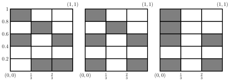
Figure 6. Left: ${\dim_{\rm H}\Lambda^{l}=\dim_{\rm B}\Lambda^{l}=\dim_{\rm Aff}\Lambda}$ middle: ${\dim_{\rm H}\Lambda^{m}<\dim_{\rm B}\Lambda^{m}=\dim_{\rm Aff}\Lambda^{m}}$ right: $\dim_{\rm H}\Lambda^{r}<\dim_{\rm B}\Lambda^{r}<\dim_{\rm Aff}\Lambda^{r}$

In the self-affine case we will define the affinity dimension which replaces the similarity dimension. However, not any of the assertions (a)-(c) hold for all self-affine sets with disjoint cylinders.

Example 6.2.

On the left-hand side Figure 6 we see three copies of the unit square. Focus on the one which is on the left-hand side. It contains six shaded rectangles of size $\frac{1}{3}\times\frac{1}{5}$. Denote their left bottom corners by $t_{1},\dots,t_{6}$ in any particular order. Then we define the IFS

$$\mathcal{F}^{l}:=\left\{f_{i}(x)=\left(\begin{array}[]{cc}\frac{1}{3}&0\\ 0&\frac{1}{5}\\ \end{array}\right)\cdot x+t_{i}\right\}_{i=1}^{6}.$$

Let $\Lambda^{l}$ be the attractor of $\mathcal{F}^{l}$. Clearly the first cylinders of $\mathcal{F}^{l}$ are the shaded rectangles on the Figure. We say that $\mathcal{F}^{l}$ and $\Lambda^{l}$ are generated by the left hand-side of the Figure 6. We define $\mathcal{F}^{m}$, $\Lambda^{m}$ and $\mathcal{F}^{r}$, $\Lambda^{r}$ respectively, generated by the rectangles in the middle and right-hand side unit squares on Figure 6. These self affine sets belongs to the family of Bedford-McMullen carpets (see [7] for more details). The linear parts are the same in each of the three systems they differ only in the translation vectors. However, $\dim_{\rm H}\Lambda^{l}=\dim_{\rm B}\Lambda^{l}=\dim_{\rm Aff}\Lambda^{l}$, $\dim_{\rm H}\Lambda^{m}<\dim_{\rm B}\Lambda^{m}=\dim_{\rm Aff}\Lambda^{m}$ and $\dim_{\rm H}\Lambda^{r}<\dim_{\rm B}\Lambda^{r}<\dim_{\rm Aff}\Lambda^{r}$, where the affinity dimension $\dim_{\rm Aff}$ plays the same rolle here as the similarity dimension in the case of self-similar sets and it will be defined in Section 6.1.

Moreover, if $d^{l}$, $d^{m}$ and $d^{r}$ are the Hausdorff dimension of $\Lambda^{l}$,$\Lambda^{m}$ and $\Lambda^{r}$ respectively, then

$$0<\mathcal{H}^{d^{l}}(\Lambda^{l})<\infty,\quad\mathcal{H}^{d^{m}}(\Lambda^{m})=\mathcal{H}^{d^{r}}(\Lambda^{r})=\infty.$$

For simplicity here we explain everything on the plane but the definitions and discussions in $\mathbb{R}^{d}$ for $d\geq 3$ are similar. (See e.g. [7, Section 9.4] for the introduction in higher dimension.)

We can define the self-affine measures exactly as we defined self-similar measures in Section 4.1. That is for a probability vector $\mathbf{p}=(p_{1},\dots,p_{m})$ the self-affine measure corresponding to $\mathcal{F}$ and $\mathbf{p}$ is

(6.2) $$\nu=\nu_{\mathcal{F},\mathbf{p}}:=\Pi_{*}(\mathbf{p}^{\mathbb{N}}).$$

6.1. Singular value function, affinity dimension, Falconer’s Theorem

Most of the basic concepts of this field were introduced by Falconer [8]. The singular value function $\phi^{s}(A)$ of a matrix $A$ is defined by

(6.3) $$\phi^{s}(A)=\begin{cases}\alpha_{\lceil s\rceil}(A)^{s-\lfloor s\rfloor}\prod_{j=1}^{\lfloor s\rfloor}\alpha_{j}(A)&\text{if }0\leq s\leq\mathrm{rank}(A),\\ |\det(A)|^{s/\mathrm{rank}(A)}&\text{if }\mathrm{rank}(A)<s,\end{cases}$$

where $\alpha_{i}(A)$ denotes the $i$th singular value of $A$. On the plane, for a non-singular matrix $A$ this is simply

(6.4) $$\phi^{s}(A):=\left\{\begin{array}[]{ll}\alpha_{1}(A),&\hbox{if $s\leq 1$;}\\ \alpha_{1}(A)\alpha_{2}^{s-1}(A),&\hbox{if $1\leq s\leq 2$;}\\ (\alpha_{1}(A)\alpha_{2}(A))^{s/2},&\hbox{if $s\geq 2$.}\end{array}\right.$$

Using the singular value function Falconer [8] defined the affinity dimension $\dim_{\rm Aff}\Lambda$ as the root of the subadditive pressure formula

(6.5) $$P_{A_{1},\dots A_{m}}(\dim_{\rm Aff}\Lambda)=0,$$

where the function $s\mapsto P_{A_{1},\dots A_{m}}(s)$ is defined in the Appendix Example B.3. This is the value of the Hausdorff dimension of $\Lambda$ in most of the cases.

Theorem 6.3 (Falconer).

Fix the $d\times d$ non-singular matrices $A_{1},\dots,A_{m}$ in any particular ways satisfying $\max\limits_{1\leq i\leq m}\|A_{i}\|<1/2$. For every $\mathbf{t}=(t_{1},\dots,t_{m})\in\mathbb{R}^{md}$ we consider the following self-affine IFS on $\mathbb{R}^{d}$: $\mathcal{F}^{\mathbf{t}}:=\left\{f_{i}(x):=A_{i}x+t_{i}\right\}_{i=1}^{m}$, where the translations $\mathbf{t}=(t_{1},\dots,t_{m})$ are considered as parameters. Then $\dim_{\rm H}\Lambda=\dim_{\rm B}\Lambda=\dim_{\rm Aff}\Lambda$ for Lebesgue almost all choices of $(t_{1},\dots,t_{m})\in\mathbb{R}^{dm}$.

7. Ergodic measures for a self-affine IFS

Let $\mathcal{F}$ be a self-affine IFS as in Definition 6.1. Then for an arbitrary ergodic measure $\nu$ on $\Sigma$ we have

(7.1) $$\chi_{k}(\nu):=\chi_{k}(\Pi_{*}\nu):=\lim\limits_{n\to\infty}\frac{1}{n}\log\alpha_{k}(A_{i_{1}}\cdots A_{i_{n}}).$$

where $\alpha_{k}(B)$ is the $k$-th singular value of the matrix $B$.

In high generality we know only almost all type formulas for the Hausdorff dimension of $\Pi_{*}\nu$. Namely, we consider the translations $\mathbf{t}=(t_{1},\dots,t_{m})$ as parameters (as in Theorem 6.3) in the self affine IFS of the form (6.1) and we write $\mathcal{F}^{\mathbf{t}}$ instead of $\mathcal{F}$, $\Pi^{\mathbf{t}}$ instead of $\Pi$ and $\Pi^{\mathbf{t}}_{*}\nu$ instead of $\Pi_{*}\nu$. Then [14, Theorem 1.9] gives an analogous assertion to Falconer’s theorem (Theorem 6.3) for self-affine measures instead of self-affine sets:

Theorem 7.1 (Jordan Pollicott and Simon).

Let $\nu$ be an arbitrary ergodic measure on $\Sigma=\left\{1,\dots,m\right\}^{\mathbb{N}}$. If $\max\limits_{1\leq i\leq m}\|A_{i}\|<1/2$ then for almost all $\mathbf{t}$ (w.r.t. the $m\cdot d$-dimensional Lebesgue measure) we have

(7.2) $$\dim_{\rm H}(\Pi^{\mathbf{t}}_{*}\nu)=\min\left\{d,D(\nu)\right\},$$

where $D(\nu)$ is the Lyapunov dimension for the ergodic measure $\nu$ defined below.

Definition 7.2.

Let $\mathcal{F}$ be a self-affine IFS as in Definition 6.1. Then for an arbitrary ergodic measure $\nu$ on $\Sigma$

(7.3) $$D(\nu):=k+\frac{h(\nu)+\chi_{1}(\nu)+\cdots+\chi_{k}(\nu)}{-\chi_{k+1}(\nu)},$$

if $k=k(\nu)=\max\left\{i:0<h(\nu)+\chi_{1}(\nu)+\cdots+\chi_{i}(\nu)\right\}\leq d$. On the other hand, if $0<h(\nu)+\chi_{1}(\nu)+\cdots+\chi_{d}(\nu)$ then we define

(7.4) $$D(\nu):=d\cdot\frac{h(\nu)}{-(\chi_{1}(\nu)+\cdots+\chi_{d}(\nu))}.$$

We call $D(\nu)$ the Lyapunov dimension of the measure $\nu$.

Example 7.3.

In this paper we mostly work on the plane ($d=2$). In this case

(7.5) $$D(\nu)=\left\{\begin{array}[]{ll}\frac{h(\nu)}{|\chi_{1}(\nu)|},&\hbox{if $h(\nu)\leq|\chi_{1}(\nu)|$ ;}\\ 1+\frac{h(\nu)-|\chi_{1}(\nu)|}{|\chi_{2}(\nu)|},&\hbox{if $|\chi_{1}(\nu)|\leq h(\nu)\leq|\chi_{1}(\nu)|+|\chi_{2}(\nu)|$;}\\ 2\cdot\frac{h(\nu)}{|\chi_{1}(\nu)|+|\chi_{2}(\nu)}|,&\hbox{if $|\chi_{1}(\nu)|+|\chi_{2}(\nu)|\leq h(\nu)$.}\end{array}\right.$$

Recently there have been a number of very significant achievements on this field. Here we mention only one of them. Bárány, Hocfhman and Rapaport [1, Theorem 1.2] computed the Hausdorff dimension of self-affine measures under some mild conditions. They obtained this by combining the entropy growth theorem by Hochman [9] with the method of Bárány and Käenmäki [2] about the dimension of the projections of self-affine measures, that they got by an application of the Furstenberg measures.

7.1. Self-affine measures

Definition 7.4.

Let $\mathcal{F}:=\left\{f_{i}(x):=A_{i}x+t_{i}\right\}_{i=1}^{m}$ be a self-affine IFS on $\mathbb{R}^{d}$ and let $\mathbf{p}$ be a probability vector. Then the corresponding self-affine measure can be defined exactly as we defined the self-similar measures. That is

(7.6) $$\nu=\nu_{\mathcal{F},\mathbf{p}}:=\Pi_{*}\left(\mathbf{p}^{\mathbb{N}}\right),$$

In their very recent seminal paper Bárány, Hochman and Rapaport [1, Theorems 1.1 and 1.2] proved the following

Theorem 7.5 (Bárány, Hochman and Rapaport).

Let $\mathcal{F}:=\left\{f_{i}(x):=A_{i}x+t_{i}\right\}_{i=1}^{m}$ be a self-affine IFS on $\mathbb{R}^{2}$ which satisfies both of the following conditions:

(a):

the strong open set condition (see Definition 4.2) and

(b):

The normalized linear parts $\left\{A_{i}/\sqrt{|\det A_{i}|}\right\}_{i=1}^{m}$ generate a non-compact and totally irreducible subgroup of $GL_{2}(\mathbb{R}^{d})$ (that is they do not preserve any finite union of non-trivial linear spaces,)

Then for an arbitrary probability vector $\mathbf{p}$ we have

(7.7) $$\dim_{\rm H}\nu_{\mathcal{F},\mathbf{p}}=D(\nu_{\mathcal{F},\mathbf{p}})\mbox{ and }\dim_{\rm H}\Lambda=\dim_{\rm B}\Lambda=\dim_{\rm Aff}\Lambda,$$

where $\Lambda$ is the attractor of $\mathcal{F}$ and we remind the reader that the affinity dimension $\dim_{\rm Aff}$ was defined in (6.5).

This theorem does not cover the case of those self affine IFS for which all of the mappings have lower triangular linear parts. However, the same authors proved in [1, Proposition 6.6]

Theorem 7.6 (Bárány, Hochman and Rapaport).

Let $\mathcal{F}:=\left\{f_{i}(x):=A_{i}x+t_{i}\right\}_{i=1}^{m}$ be a self-affine IFS on $\mathbb{R}^{2}$ which satisfies both of the following conditions:

(c):

The linear parts of all of the mapping of $\mathcal{F}$ are lower triangular:
$A_{i}=\left(\begin{array}[]{cc}a_{i}&0\\ b_{i}&c_{i}\\ \end{array}\right)$ for $i=1,\dots,m$ and

(d):

$a_{i}<c_{i}$ for all $i=1,\dots,m$.

Then for an arbitrary probability vector $\mathbf{p}$ we have

(7.8) $$\dim_{\rm H}\nu_{\mathcal{F},\mathbf{p}}=D(\nu_{\mathcal{F},\mathbf{p}})\mbox{ and }\dim_{\rm H}\Lambda=\dim_{\rm B}\Lambda=\dim_{\rm Aff}\Lambda,$$

where $\Lambda$ is the attractor of $\mathcal{F}$.

8. Ergodic measures for Barnsley’s skew product maps

We use the notation of Section 2. Let $\mu$ be an ergodic measure for the Barnsley’s skew product map $F$, which was defined in Section 2. The two Lyapunov exponents $\chi_{1}(\mu)$ and $\chi_{2}(\mu)$ of $F$ are

$$\chi_{x}(\mu)=\int\log\|D_{\mathrm{proj}(\mathbf{x})}f\|\mathrm{d}\mu(\mathbf{x})=\sum_{i=1}^{m}\mu(I_{i}\times\mathbb{R})\log\gamma_{i}\text{ and }$$

$$\chi_{y}(\mu)=\int\log\|\partial_{2}g(\mathbf{x})\|\mathrm{d}\mu(\mathbf{x})=\sum_{i=1}^{m}\mu(I_{i}\times\mathbb{R})\log\lambda_{i},$$

where $\mathrm{proj}(\mathbf{x})$ is the orthogonal projection of an $\mathbf{x}\in D$ to the $x$-axis and $\partial_{2}$ means the derivative with respect to the second coordinate.

Remark 8.1.

If $0<\chi_{x}(\mu)\leq\chi_{y}(\mu)$ then

$$\dim\mu=\frac{h(\mu)}{\chi_{x}(\mu)},$$

Namely, the upper bound is trivial and the lower bound follows from the fact that $\mathrm{proj}_{*}\mu$ is $f$-invariant and ergodic and the result of Hofbauer and Raith [11, Theorem 1] (see (5.4)). That is why we can restrict ourselves to the case when

(8.1) $$\chi_{1}(\mu):=\chi_{x}(\mu)=\sum_{i=1}^{m}\mu(I_{i}\times\mathbb{R})\log\gamma_{i}>\chi_{2}(\mu):=\chi_{y}(\mu)=\sum_{i=1}^{m}\mu(I_{i}\times\mathbb{R})\log\lambda_{i}>0.$$

In this case the best guess for the dimension of the $\mu$ is the so-called Lyapunov dimension to be defined below.

Definition 8.2.

Let $\mu\in\mathcal{E}_{F}(\Lambda)$ satisfying $\chi_{x}(\mu)>\chi_{y}(\mu)>0$. We define the Lyapunov dimension

(8.2) $$D(\nu):=\left\{\begin{array}[]{ll}\frac{h(\nu}{\chi_{y}(\nu)},&\hbox{if $h(\nu)\leq\chi_{y}(\nu)$ ;}\\ 1+\frac{h(\nu)-\chi_{y}(\nu)}{\chi_{x}(\nu)},&\hbox{if $\chi_{y}(\nu)\leq h(\nu)\leq\chi_{x}(\nu)+\chi_{y}(\nu)$;}\\ 2\cdot\frac{h(\nu)}{\chi_{x}(\nu)+\chi_{y}(\nu)},&\hbox{if $\chi_{x}(\nu)+\chi_{y}(\nu)\leq h(\nu)$.}\end{array}\right.$$

9. Hofbauer’s Pressure

In the previous sections (and in the appendix) we presented the dimension theory for the self-affine iterated function systems. However, the principal distinction of the Barnsley’s maps from the iterated function systems lies in the fact that the symbolic space for the Barnsley’s skew product map is not a full shift. In this section we will present the most general version of thermodynamical formalism theory, developed in a series of papers by Franz Hofbauer with his co-authors. This theory is not completely general, it assumes the system comes form piecewise monotone maps of the interval, but this assumption is satisfied in our situation.

Let us remind the notations. Our base map $f:[0,1]\to[0,1]$ is piecewise monotone: we can divide the interval $[0,1]$ into finitely many closed intervals with disjoint interiors $[0,1]=\bigcup_{1}^{m}I_{i}$. We denote by $\mathfrak{S}$ the set of endpoints of intervals $I_{i}$. We assume that $f|_{I_{i}^{o}}$ is continuous and monotone (strictly increasing or strictly decreasing) on $I_{i}^{o}$. We define $f_{i}$ as the extension of $f|_{I_{i}^{o}}$ by continuity to the endpoints of $I_{i}$.

In order that the symbolic expansion of the system (to be defined below) is compact, we need to take a formal modification of the maps. We would like to consider $f_{i}$ as the restriction of $f$ to $I_{i}$. Naturally, such a definition can in general lead to the map being doubly defined on some points in $\mathfrak{S}_{\infty}$, but this set is countable. Formally speaking, if for a point $x\in\mathfrak{S}$ the left and right limits of $f$ disagree then we define $f(x_{-})=\lim_{z\nearrow x}f(z)$ and $f(x_{+})=\lim_{z\searrow x}f(z)$. We then proceed to inductively double all the preimages of $x$. For a point $y\in f^{-1}(x),y\notin\mathfrak{S}$ we define: if $f$ is increasing at $y$ then $f(y-)=x_{-}$ and $f(y_{+})=x_{+}$, otherwise $f(y-)=x_{+}$ and $f(y_{+})=x_{-}$. And for a point $y\in f^{-1}(x),y\in\mathfrak{S}$: if $\lim_{z\nearrow y}f(z)=x$ and $f$ is increasing in $(y-\varepsilon,y)$ then $f(y_{-})=x_{-}$, if it is decreasing then $f(y_{-})=x_{+}$, if $\lim_{z\searrow y}f(z)=x$ and $f$ is increasing in $(y,y+\varepsilon)$ then $f(y_{+})=x_{+}$, if it is decreasing then $f(y_{+})=x_{-}$. We set the natural topology: at each doubled point $x$ $\lim_{z\nearrow x}z=x_{-},\lim_{z\searrow x}z=x_{+}$. We also redefine the partition intervals: if $I_{i}=[x,y]$ and one or both of the endpoints are doubled then we set $I_{i}=[x_{+},y_{-}]$.

Observe that the resulting set is not an interval anymore, but a Cantor set - but with a natural projection onto the interval, which is 2-1 on a countable set and 1-1 elsewhere. The well-known special case of this construction: consider the interval $[0,1]$ with the map $f(x)=2x(\mod 1)$ and divide each dyadic point into two. That is, $1/2=0.10000..._{2}=0.01111..._{2}$, we formally define $(1/2)_{-}=0.01111..._{2}$ and $(1/2)_{+}=0.10000..._{2}$ – and the same for all the other dyadic points. The result is a full shift on two symbols, which is conjugate (modulo a countable set) to the original map.

Note that for the piecewise monotone map the minimal possible partition is given by the intervals of monotonicity of $f$, but we can freely subdivide the intervals $I_{i}$ further, and the resulting maps will also belong to considered class. In particular, we can freely demand that for any given continuous potential $\varphi:[0,1]\to\mathbb{R}$ its variation $\sup\varphi-\inf\varphi$ is arbitrarily small on each $I_{i}$.

Let $A$ be a compact, $f$-invariant, $f$-transitive set. For the rest of the section, our dynamical system will be the restriction of $f$ to $A$.

Let $\widetilde{\Sigma}\subset\{1,\ldots,m\}^{\mathbb{N}}$ be the symbolic system of our dynamics, defined as the set of sequences $\omega\in\{1,\ldots,m\}^{\mathbb{N}}$ such that there exists $x\in A$ such that for $n=0,1,\ldots$

$$f^{n}(x)\in I_{\omega_{n}}.$$

One can check that $\widetilde{\Sigma}$ is a subshift, that is a $\sigma$-invariant and closed subset of $\{1,\ldots,f\}^{\mathbb{N}}$. The sequence $\omega$ will be called symbolic expansion of $x$, $x$ will be called representation of $\omega$. We will write $x=\pi(\omega)$. We will assume the partition $\{I_{i}\}$ is generating, that is each $\omega\in\widetilde{\Sigma}$ has unique representation. This always holds if $f$ is expanding.

For any finite word $\tau^{n}\in\{1,\ldots,m\}^{n}$ denote by $C[\tau^{n}]$ the set of points $x\in A$ such that $\pi^{-1}(x)$ begins with $\tau^{n}$. This set will be called $n$-th level cylinder. The set of $n$-th level cylinders will be denoted $D_{n}$. For $x\in A$, let $C_{n}(x)$ be the $n$-th level cylinder containing $x$. Denote $d_{n}(x)=\mathrm{diam}C_{n}(x)$ and $\varphi_{n}(x)=\sup\{\varphi(y)-\varphi(z);y,z\in C_{n}(x)\}$. We have

$$\lim_{n\to\infty}d_{n}(x)=\lim_{n\to\infty}\varphi_{n}(x)=0.$$

Definition 9.1.

We say that $A$ is Markov if there exists such partition $\{I_{i}\}$ and such $n$ that for every $n$-th level cylinder $C[\tau^{n}]$ its image $T(C[\tau^{n}])$ is a union of $n$-th level cylinders. Equivalently, $A$ is Markov if for some partition $\{I_{i}\}$ the subshift $\widetilde{\Sigma}$ is a subshift of finite type, that is a subshift defined as all the infinite words $\omega\in\{1,\ldots,m\}^{\mathbb{N}}$ that do not contain any word from some finite list of finite words.

9.1. Pressure and Markov sets

Let $\varphi:[0,1]\to\mathbb{R}$ be a piecewise continuous potential, with the set of discontinuities contained in $\mathfrak{S}$. For the Markov systems we can define the pressure in the usual way:

(9.1) $$P(A,\varphi)=\lim_{n\to\infty}\frac{1}{n}\log\sum_{C[\omega^{n}]\in D_{n}}\exp(\sup_{x\in C[\omega^{n}]}S_{n}\varphi(x)),$$

compare (A.17). For the non-Markov systems the right hand side of this equation is still well-defined, but is considered too large for applications in dimension theory. Let us give a short explanation.

In the year 1973 Rufus Bowen [3] gave the following definition of topological entropy: given a continuous map $f:X\to X$, where $X$ is any $f$-invariant set (not necessarily compact), let $X_{n}$ be the $n$-th level cylinders, then

$$h_{\rm top}(f,X)=\inf\{s;\inf_{X\subset\bigcup E_{i}}\sum e^{-sn(E_{i})}=0\},$$

where the sum is taken over covers of $X$ with cylinders and for a cylinder $E$ $n(E)$ denotes its level. Geometrically, the Bowen’s definition of topological entropy is similar to the Hausdorff dimension as the usual definition (A.8) is similar to the box counting dimension – or more precisely, the Bowen’s definition is the Hausdorff dimension and (A.8) is the box counting dimension, both calculated in a special metric (so-called dynamical metric). Still, Bowen proved that for compact $X$ the two definitions are equal, while for noncompact the Bowen’s definition gives in general a smaller number. For example, for a countable set $X$ the Bowen’s entropy is always 0.

Our set $A$ is compact, so there is no disagreement about what $h_{\rm top}(f,A)$ is. However, even though the pressure is heuristically a very similar object to the topological entropy (in both cases we are just counting how many trajectories the system has, except in the case of pressure we count the trajectories with some weights, given by the potential), there is no analogue of Bowen’s theorem. Thus, we can always define the pressure by formula (9.1), but it is only an upper bound for the correct formula – which we do not know.

Except for the Markov systems. For a Markov system each $n$-th level cylinder is large, in the sense that there exists $\delta>0$ such that for every $C[\omega^{n}]\in D_{n}$ we have

$$\mathrm{diam}f^{n}(C[\omega^{n}])>\delta.$$

It is not necessarily so for non-Markov systems: some $n$-th level cylinders might be very tiny (they will be not only $n$-th level cylinders but also $n+1,\ldots,n+\ell$-th level cylinders, for some possibly large $\ell$). As the result, the sum on the right hand side of (9.1) overstates their importance (counting them as $n$-th level cylinders while they would be counted as $n+\ell$-th level cylinders by Bowen). Thus, Franz Hofbauer in [10] gave a better definition of pressure:

(9.2) $$P(A,\varphi)=\sup_{B\subset A,B{\rm Markov}}P(B,\varphi),$$

where $P(B,\varphi)$ is given by (9.1). For Markov $A$ (9.2) gives the same value as (9.1). We note that it is still an open question whether the formula (9.2) can be strictly smaller than (9.1) for non-Markov $A$.

9.2. Conformal measure and small cylinders

We finish the section with two more important results of Franz Hofbauer. The first of them was obtained together with Mariusz Urbański [12]. We will call a probabilistic measure $\mu$ defined on $A$ conformal for the potential $\varphi$ if for every $n$ and for every $C[\omega^{n}]\in D_{n}$ we have

$$\mu(TC[\omega^{n}])=\int_{C[\omega^{n}]}e^{P(A,\varphi)-\varphi}d\mu.$$

As the partition is generating, this formula can be iterated:

$$\mu(T^{n}C[\omega^{n}])=\int_{C[\omega^{n}]}e^{nP(A,\varphi)-S_{n}\varphi}d\mu.$$

Theorem 9.2 (Hofbauer, Urbański).

Let $A$ be topologically transitive, compact, $T$-invariant set of positive entropy. Then for every piecewise continuous potential $\varphi$ there exists a nonatomic conformal measure $\mu(A,\varphi)$ with support $A$.

The second result of Hofbauer, from [10], provides a way of estimating the set of points $x\in A$ such that for every $n$ the cylinder $C_{n}(x)$ is not large. Denote

$$N_{\rho}(A,\mu)=\{x\in A;\limsup_{n\to\infty}\mu(T^{n}C_{n}(x))\leq\rho\}.$$

Denote also by $D(\alpha)$ the set of points $x\in A$ with Lyapunov exponent $\alpha$. We remind that $\varphi_{1}(x)$ denotes the variation of potential $\varphi$ in first level cylinder containing $x$.

Lemma 9.3 (Hofbauer).

For every $\alpha>\sup_{x}(\log|F^{\prime}|)_{1}(x)$,

$$\lim_{\rho\to 0}\dim_{H}(N_{\rho}\cap D(\alpha))=0.$$

We note that $\sup_{x}(\log|F^{\prime}|)_{1}(x)$ can be arbitrarily decreased by considering subpartitions of $\{I_{i}\}$.

10. The dimension of Barnsley’s repellers

First we recall the basic definitions.

10.1. The basic definitions

First we recall the definition of Barnsley’s skew product maps: Given $\left\{I_{i}\right\}_{i=1}^{m}$ which is a partition of $[0,1]$. Let $D_{i}:=I_{i}\times\mathbb{R}$. For $(x,y)\in D_{i}$ we defined $F_{i}(x,y):=(f_{i}(x),g_{i}(x,y))$, where $f_{i}:I_{i}\to J_{i}\subset[0,1]$ onto, and

(10.1) $$f_{i}(x):=\gamma_{i}x+v_{i},\ g_{i}(x,y)=a_{i}x+\lambda_{i}y+t_{i},\ |\lambda_{i}|,|\gamma_{i}|>1,\quad t_{i},v_{i}\in\mathbb{R}.$$

Also recall that we define $f(x):=f_{i}(x)$ if $x\in I_{i}$. The set of admissible words is defined as

(10.2) $$X:=\mathrm{cl}\left\{(i_{1},i_{2},\dots)\in\Sigma:\exists x\in I\text{ such that }\forall n\geq 0,\ f^{n}(x)\in I_{i_{n}}^{o}\right\},$$

where $\mathrm{cl}(A)$ is the closure of the set $A\subset\Sigma:=\left\{1,\dots,m\right\}^{\mathbb{N}}$ in the usual topology on $\Sigma$.

Definition 10.1.

We say that $f$ is Markov if $f(\overline{I_{i}})$ is equal to a finite union of elements in $\{\overline{I_{i}}\}_{i=1}^{m}$ for every $i=1,\ldots,m$.

10.2. Diagonal and essentially non-diagonal system

Since the maps $F_{i}$ are affine the derivatives $DF_{i}$ are constant lower triangular matrices

$$DF_{i}:=\left(\begin{array}[]{cc}\gamma_{i}&0\\ a_{i}&\lambda_{i}\\ \end{array}\right).$$

However, it is very important if the derivative matrices are diagonal or essentially non diagonal along the dynamics since the proofs that work for the essentially non-diagonal case do not work for the diagonal ones and we need different assumptions in these different cases.

Definition 10.2.

We say that

(a):

$F$ is diagonal if all the matrices $DF_{i}$ are diagonal.

(b):

$F$ is essentially diagonal if the system of matrices $\left\{DF_{i}\right\}_{i=1}^{m}$, simultaneously diagonizable. This holds if

(10.3) $$\frac{\gamma_{i}-\lambda_{i},}{a_{i}}=\frac{\gamma_{j}-\lambda_{j}}{a_{j}},\quad\forall i,j\in\left\{1,\dots,m\right\}.$$

(c):

$F$ is essentially non-diagonal along the dynamics if there are admissible words $\boldsymbol{\omega},\boldsymbol{\tau},\in X$ and another word $\boldsymbol{\eta}$ such that $\boldsymbol{\omega}\boldsymbol{\eta}\boldsymbol{\tau}\in X$ such that

1. both $f_{\boldsymbol{\omega}}$ and $f_{\boldsymbol{\tau}}$ have fixed points

2. $\left\{DF_{\boldsymbol{\omega}},DF_{\boldsymbol{\tau}}\right\}$ are not simultaneously diagonizable. That is for

   $$DF_{\boldsymbol{\omega}}=\left(\begin{array}[]{cc}\gamma_{\boldsymbol{\omega}}&0\\ a_{\boldsymbol{\omega}}&\lambda_{\boldsymbol{\omega}}\\ \end{array}\right)\quad\mbox{ and }\quad DF_{\boldsymbol{\tau}}=\left(\begin{array}[]{cc}\gamma_{\boldsymbol{\tau}}&0\\ a_{\boldsymbol{\tau}}&\lambda_{\boldsymbol{\tau}}\\ \end{array}\right)$$

   we have

   $$\frac{\gamma_{\boldsymbol{\omega}}-\lambda_{\boldsymbol{\omega}}}{a_{\boldsymbol{\omega}}}\neq\frac{\gamma_{\boldsymbol{\tau}}-\lambda_{\boldsymbol{\tau}}}{a_{\boldsymbol{\tau}}}.$$

The reason for this restrictive definition in (c) is that during the proof we approximate by Markov sub-systems and we need to guarantee that even the approximating Markov sub-system remains essentially non-diagonal.

10.3. Markov pressure and Hofbauer Pressure

Using the notation of (2.3), we introduce potential:

(10.4) $$\varphi^{s}(x)=\begin{cases}-s\log|\lambda_{i}|&\text{if }0\leq s\leq 1,\\ -\left(\log|\lambda_{i}|+(s-1)\log|\gamma_{i}|\right)&\text{if }1<s\leq 2.\end{cases}$$

Definition 10.3 ($P(s,B)$).

Let $s>0$ and $B\subset[0,1]$ be a Markov subset. Recall that in (9.1) we defined the pressure $P(B,\varphi)$ for Markov subset $B\subset[0,1]$ and potential $\varphi$. Using this definition we can define

(10.5) $$P(s,B):=P(B,\varphi^{s}).$$

The following lemma helps to get better understanding:

Lemma 10.4.

Assume that $B\subset[0,1]$ is Markov of type-1 set. That is for every $i,j\in\left\{1,\dots,m\right\}$ either $I_{j}\cap B\subset f(I_{i}\cap B)$ or $(I_{j}\cap B)\cap f(I_{i}\cap B)=\emptyset$. Then

$$A_{i,j}^{(s)}=\begin{cases}(1/\lambda_{i})\cdot(1/\gamma_{i})^{s-1}&\text{if }I_{j}\cap B\subseteq f(I_{i}\cap B)\\ 0&\text{otherwise.}\end{cases}$$

Then $P(s,B)=\log\rho(A^{(s)})$, where $\rho(A)$ denotes the spectral radius of $A$.

We remark that every subshifts of type-$n$ can be corresponded to a type-1 subshift by defining a new alphabet, and subdividing the monotonicity intervals into smaller intervals.

Definition 10.5 ($P_{\mathrm{Mar}}(s),P_{\mathrm{Hof}}(s)$).

Now we define the functions $s\mapsto P_{\mathrm{Mar}}(s)$ and $s\mapsto P_{\mathrm{Hof}}(s)$ as follows:

(a):

If $f$ is Markov then we write $P_{\mathrm{Mar}}(s):=P(s,[0,1])$

(b):

If $f$ is none Markov then we write

(10.6) $$P_{\mathrm{Hof}}(s):=\sup\limits_{B\subset[0,1],\ B\ \mathrm{Markov}}P(s,B).$$

10.4. The main results

Theorem 10.6.

Suppose that

(a):

$F$ is essentially diagonal,

(b):

$\gamma_{i}>\lambda_{i}$ for every $i=1,\ldots,m$,

(c):

The self-similar IFS $\{g_{i}^{-1}(y)=\frac{y-t_{i}}{\lambda_{i}}\}_{i=1}^{M}$ satisfies HESC (see Condition 4.10)

then

$$\dim_{H}\Lambda=\dim_{B}\Lambda=\sup_{\mu\in\mathcal{M}_{\rm{erg}}(\Lambda)}D(\mu)=s_{0},$$

where $s_{0}$ is the unique number such that

• $P_{\mathrm{Mar}}(s_{0})=0$ if $f$ is Markov, otherwise

• $P_{\mathrm{Hof}}(s_{0})=0$.

.

Theorem 10.7.

Assume that $F$ is essentially non-diagonal and $f$ is a topologically transitive. If $\gamma_{i}>\lambda_{i}$ for every $i=1,\ldots,m$ then

$$\dim_{H}\Lambda=\dim_{B}\Lambda=\sup_{\mu\in\mathcal{M}_{\rm{erg}}(\Lambda)}D(\mu)=s_{0},$$

where $s_{0}$ is the unique number such that

• $P_{\mathrm{Mar}}(s_{0})=0$ if $f$ is Markov, otherwise

• $P_{\mathrm{Hof}}(s_{0})=0$.

Appendix A Thermodynamical formalism

First we introduce the subshift of finite type.

A.1. Subshift of finite type

Let ${\Sigma=\left\{1,\dots,m\right\}^{\mathbb{N}}}$ be endowed with the usual topology, which generated by the distance $\mathrm{dist}(\mathbf{i},\mathbf{j}):=m^{-\left|\mathbf{i}\wedge\mathbf{j}\right|}$, where

$$\left|\mathbf{i}\wedge\mathbf{j}\right|=\max\left\{n:\forall|\ell|\leq n,i_{\ell}=j_{\ell}\right\}.$$

For some $k<r$ we write ${\left[\mathbf{i}\right]_{k,r}=\left\{\mathbf{j}\in\Sigma:i_{\ell}=j_{\ell},\ \forall\ell\in\left\{k,\dots,r\right\}\right\}}$ for the $(k,r)$ cylinder sets. If $k=1$ then we write simply $[\mathbf{i}]_{r}$. Similarly,

$$[i_{1},\dots,i_{n}]:=\left\{\mathbf{j}\in\Sigma:i_{k}=j_{k},\forall k=1,\dots,n\right\}.$$

For an $\mathbf{i}\in\Sigma$ we write

(A.1) $$\mathbf{i}|_{n}:=(i_{1},\dots,i_{n})\in(1,\dots,m)^{n}=:\Sigma_{n}.$$

Definition A.1 (subshift of finite type).

Given an $m\times m$ matrix $A$ of $0$’s and $1$’s. Let  $\Sigma_{A}:=\left\{\mathbf{i}\in\Sigma:A_{i_{k},i_{k+1}}=1,\ \forall k\in\mathbb{N}\right\}$ and let $\sigma$ be the left shift on $\Sigma_{A}$. That is $\sigma(i_{1},i_{2},i_{3}\dots):=(i_{2},i_{3}.\dots)$ for every $(i_{0},i_{1},i_{2},\dots)\in\Sigma_{A}$. Clearly, $\sigma(\Sigma_{A})=\Sigma_{A}$ and $\sigma|_{\Sigma_{A}}$ is a homeomorphism on $\Sigma_{A}$. Sometimes we call $\sigma|_{\Sigma_{A}}$ topological Markov chain.

We always assume that for every $k\in\left\{1,\dots,m\right\}$ there exist some $\mathbf{i}\in\Sigma_{A}$ such that $i_{0}=k$. From now on we call

• $(\Sigma,\sigma)$ a full shift and

• $(\Sigma_{A},\sigma)$ as subshift of finite type.

Also for the rest of this Section we assume that $A$ is an $m\times m$ primitive matrix.

$${\Sigma_{A,n}:=\left\{\mathbf{i}=(i_{1},\dots,i_{n}):[i_{1},\dots,i_{n}]\cap\Sigma_{A}\neq\emptyset\right\}}.$$

A.2. Ergodic measures

Given a measurable self-map $T$ of a measurable space $(X,\mathcal{B})$. That is $T:X\to X$ and $T^{-1}B\in\mathcal{B}$ for every $B\in\mathcal{B}$. We write

• $\mathcal{M}(X)$ for the set of Borel probability measures on $(X,\mathcal{B})$,

• $\mathcal{M}_{T}(X)$ for the set of invariant measures. That is
  

  $$\mathcal{M}_{T}(X)=\left\{\mu\in\mathcal{M}(X):\mu(A)=\mu(T^{-1}A),\ \forall A\in\mathcal{B}\right\},$$

• $\mathcal{E}_{T}(X)$ for the ergodic measures. That is

  $$\mathcal{E}_{T}(X)=\left\{\mu\in\mathcal{M}_{T}(X):A=T^{-1}A\Longrightarrow\mbox{ either }\mu(A)=0,\mbox{ or }\mu(A)=1\right\}.$$

We frequently use Birkhoff’s Ergodic Theorem.

Theorem A.2 (Birkhoff’s Ergodic Theorem).

Let $\mu\in\mathcal{E}_{T}(X)$ and let $f\in L^{1}(X,\mu)$. Then for $\mu$-almost all $x\in X$ the ergodic averages converge both in $L^{1}$ and pointwise:

(A.2) $$\lim\limits_{n\to\infty}\frac{1}{n}\sum\limits_{k=0}^{n-1}f(T^{k}(x))=\int f(x)d\mu(x).$$

A.3. Entropy

One of the basic concepts of the thermodynamical formalism is the entropy. There is measure theoretical and topological entropy. Here we just present the definitions and a basic property. For further reading we recommend [4], [22] and a very detailed introduction is given in [20].

A.3.1. Measure theoretical entropy on $(\Sigma_{A},\sigma)$ for an ergodic measure

First we define the measure theoretical entropy on $\Sigma_{A}$ for an ergodic (with respect to the left shift $\sigma$) measure. (We always assume that $A$ is a primitive matrix.)

Definition A.3 (Entropy (measure theoretical)).

Let $\mu$ be an ergodic measure on $\Sigma_{A}$. We can define the entropy of $\mu$ as

(A.3) $$h(\mu):=\lim\limits_{n\to\infty}\frac{1}{n}\sum\limits_{\boldsymbol{\omega}\in{\Sigma_{A,n}}}\mu([\boldsymbol{\omega}])\log\mu([\boldsymbol{\omega}]).$$

Theorem A.4 (Shannon Breiman McMillian Theorem).

Let $\mu\in\mathcal{E}_{\sigma}(\Sigma)$. Then for $\mu$-almost all $\mathbf{i}\in\Sigma_{A}$ we have

(A.4) $$\lim\limits_{n\to\infty}\frac{1}{n}\log\mu[\mathbf{i}|_{n}]=h(\mu).$$

For the proof see [4].

Example A.5.

(a):

Bernoulli shift. Given a probability vector $\mathbf{p}:=(p_{1},\dots,p_{m})$, where $p_{i}$ and $\sum\limits_{i=1}^{m}p_{i}=1$.Then we say the $\mu:=\mathbf{p}^{\mathbb{N}}$ is the Bernoulli measure corresponding to $\mathbf{p}$. It is easy to see that

(A.5) $$h(\mu)=-\sum\limits_{i=1}^{m}p_{i}\log p_{i}.$$

(b):

Markov Shift Given a stochastic matrix $P=(p_{i,j})_{1\leq i,j\leq m}$. That is $\sum\limits_{j=1}^{m}p_{i,j}=1$, $p_{i,j}\geq 0$. We assume that $P$ is primitive (it was enough to assume less). Then by Perron Frobenius Theorem there exists a left eigenvector $\mathbf{p}=(p_{1},\dots,p_{m})$ which is a probability vector, such that $\mathbf{p}^{T}\cdot P=\mathbf{p}^{T}$, ($\mathbf{p}$ is considered as a column vector). We define the Markov measure $\mu$ on $\Sigma$ corresponding to $(\mathbf{p},P)$ by $\mu([\boldsymbol{\omega}]):=p_{\omega_{1}}\cdot p_{\omega_{1},\omega_{2}}\cdots p_{\omega_{n_{1}},\omega_{\omega_{n}}}$, where $\boldsymbol{\omega}\in\Sigma_{n}$ and $\boldsymbol{\omega}=(\omega_{1},\dots,\omega_{n})$. Then

(A.6) $$h(\mu)=-\sum\limits_{i,j=1}^{m}p_{i}p_{i,j}\log p_{i,j}$$

(c):

Parry measure Let $A=(a_{i,j})_{1\leq i,j\leq m}^{m}$ be an primitive matrix (to assume irreduciblity was enough again) whose entries belong to $\left\{0,1\right\}$. Then we define the canonical Markov measure as follows: Let $\lambda$ be the largest (Perron-Frobenius) eigenvalue. Let $\mathbf{u}:=(u_{1},\dots,u_{m})$ and $\mathbf{v}:=(v_{1},\dots,v_{m})$ be the left and right (positive) eigenvectors satisfying $\sum\limits_{i=1}^{m}u_{i}=1$ and $\sum\limits_{i=1}^{m}u_{i}v_{i}=1$ (see [22, p. 16]). Then we define

(A.7) $$p_{i}:=u_{i}v_{i}\mbox{ and }\quad p_{i,j}:=\frac{a_{i,j}v_{j}}{\lambda v_{i}}$$

Let $\mu$ be the Markov measure corresponding to $(\mathbf{p},P)$. Then the unique measure on $\Sigma_{A}$ with maximal entropy is $\mu$ and $h(\mu)=\log\lambda$.

A.3.2. Topological entropy on compact metric spaces for continuous mappings

Now we give the definition of the topological entropy in a more general setup (see e.g. [5, p. 165-170] ).

Definition A.6 (Topological entropy).

Given a homeomorphism $T$ of the compact metric space $(X,d)$. For $\varepsilon>0$ we say the orbits of length $n$

$${x,T(x),\dots,T^{n-1}(x)}\mbox{ and }{y,T(y),\dots,T^{n-1}(y)}$$

are the same with $\varepsilon$-precision if

$${d(T^{i}(x),T^{i}(y))<\varepsilon,\quad\forall i=0,\dots,n-1}.$$

Fix an $\varepsilon>0$ and an $n\in\mathbb{N}$. Let ${s_{n}(x,\varepsilon)}$ be the maximal number of $n$-orbits which are different with $\varepsilon$-precision. Then we define the topological pressure of $T$ by

(A.8) $${{h_{\mathrm{top}}(T)=\lim\limits_{\varepsilon\to 0}\limsup\limits_{n\to\infty}\frac{1}{n}\log s_{n}(\varepsilon)}}$$

We remark that this is not the most common way to define the topological entropy.

Theorem A.7.

Let $T:X\to X$ be a contiuous map of a compact metric space. then $h_{\mathrm{top}}(T)=\sup\left\{h_{T}(\mu):\mu\mbox{ is an invariant measure for }T\right\}$.

We defined the measure theoretical entropy only on subshift of finite type. The definition in the general case is similar see e.g. [4] and [22]. Before we give some examples we need the following definition that will also be used later.

Definition A.8.

Let $T:I\to I$, where $I\subset\mathbb{R}$ is an interval.

• We say that $T$ is a piecewise monotone map if there is a finite partition of $I$ such that on every class of this partition the map $T$ is monotone.

• Let $T$ be a piecewise monotone map. The the lap number ${\ell(T)}$ is the number of maximal monotonicity intervals of $T$.

Example A.9.

(a):

For a subshift of finite type $(\Sigma_{A},\sigma)$ the topological entropy of $\sigma$ is $\log\lambda$, where $\lambda$ is the largest eigenvalue of the primitive $0,1$ matrix $A$.

(b):

Here we use the notation of Definition A.9. It follows from a theorem of Misiurewicz and Szlenk that for a piecewise monotone map $T$, we have

(A.9) $$h(T)=\lim\limits_{n\to\infty}\frac{1}{n}\log\ell(T^{n}),$$

where $T^{n}$ is the $n$-fold composition of $T$. In particular, $h(T)\leq\ell(T)$. Moreover, if $T$ is piecewise affine and its the slope of $\pm s$ at every point (except the turning points) then $h(T)=\max\left\{0,\log s\right\}$.

(See [5] for the proofs.)

A.4. Lyapunov exponent

To define the Lyapunov exponents we need Oseledec Theorem. The following version of Oseledec Theorem is from Krengel’s book [16, p. 42-47] where the proof is also presented. Given a finite measure space $(\Omega,\mathcal{A},\mu)$ and $\tau:\Omega\to\Omega$ measure preserving. Further, $M$ denotes the set of $r\times r$ matrices. Put

$$P_{n}(A,\omega):=A(\tau^{n-1}\omega)\cdots A(\tau\omega)A(\omega).$$

Theorem A.10 (Oseledec).

Legyen $A:\Omega\to M$ be measurable and we assume that

(A.10) $$\log^{+}\|A(\cdot)\|\in L_{1}(\mu).$$

Then there exists an invariant $\Omega^{\prime}\subset\Omega$ which has full $\mu$-measure such that

1. $$\lim\limits_{n\to\infty}\left(P^{*}_{n}(A,\omega)\cdot P_{n}(A,\omega)\right)^{1/2n}=:\Lambda(\omega)$$

   exists and $\Lambda$ is a symmetric positive semidefinite matrix.

2. Let $\exp(\lambda_{1}(\omega))>\cdots>\exp(\lambda_{s}(\omega))$ are the different eigenvalues of $\Lambda$ and let $E_{\nu}$ be the eigenspace of $\Lambda$ which belongs to $\exp\lambda_{\nu}(\omega)$. Then for

   $$H_{\nu}(\omega):=E_{s}(\omega)\bigoplus E_{s-1}(\omega)\bigoplus\cdots\bigoplus E_{s+1-\nu}(\omega)$$

   we have

   (A.11) $$\lim\limits_{n\to\infty}\frac{1}{n}\log\|P_{n}(A,\omega)\mathbf{v}\|=\lambda_{s+1-\nu}(\omega),\qquad\forall\mathbf{v}\in H_{\nu}(\omega)\setminus H_{\nu-1}(\omega),$$

   where $H_{0}(\omega)\equiv\emptyset$.

3. $\omega\mapsto{\rm dim}E_{\nu}(\omega)$ and $\omega\mapsto\lambda_{\nu}(\omega)$ are $\tau$-invariant maps and we call ${\rm dim}E_{\nu}(\omega)$ the multiplicity of $\lambda_{i}(\omega)$.

Definition A.11 (Lyapunov exponenets).

Let $\mu$ be an ergodic measure. Then it follows from (3) that for all $i=1,\dots,s$ and for $\mu$-almost all $\omega\in\Omega$, $\lambda_{i}(\omega)$ and ${\rm dim}E_{\nu}(\omega)$ are constants that we call $\lambda_{i}$ and $d_{i}$ respectively, for $1,\dots,s$. We partition the index set

(A.12) $$\left\{1,\dots,r\right\}=\bigsqcup\limits_{k=1}^{s}\mathcal{I}_{k},\quad\mathcal{I}_{k}:=\left\{d_{1}+\cdots+d_{k-1}+1,\cdots,d_{1}+\cdots+d_{k-1}+d_{k}\right\}$$

Then we define the Lyapunov exponents $\chi_{1}\geq\chi_{2}\geq\cdots\geq\chi_{r}$ as follows:

(A.13) $$\underbrace{\chi_{1}=\cdots=\chi_{d_{1}}}_{:=\lambda_{1}}>\underbrace{\chi_{d_{1}+1}=\cdots=\chi_{d_{1}+d_{2}}}_{:=\lambda_{2}}>\underbrace{\chi_{d_{1}+d_{2}+1}=\cdots=\chi_{d_{1}+d_{2}+d_{3}}}_{:=\lambda_{3}}>\cdots\\ >\underbrace{\chi_{d_{1}+\cdots+d_{s-2}+1}=\cdots=\chi_{d_{1}+\cdots+d_{s-2}+d_{s-1}}}_{:=\lambda_{s-1}}>\underbrace{\chi_{d_{1}+\cdots+d_{s-1}+1}=\cdots=\chi_{d_{1}+\cdots+d_{s-1}+d_{s}}}_{:=\lambda_{s}}.$$

A.5. Topological pressure and Gibbs measure

In this section we always assume that $A$ is a primitive $m\times m$ matrix and we consider the topological Markov chain (or subshift of finite type ) $(\sigma,\Sigma_{A})$ as defined in Definition A.1

Definition A.12 (Hölder continuity).

We say that a function $\phi:\Sigma_{A}\to\mathbb{R}$ is Hölder continuous  if there exists $b>0$ and $\alpha\in(0,1)$ such that

(A.14) $${\mathrm{var}_{k}\phi:=\sup\left\{\left|\phi(\mathbf{i})-\phi(\mathbf{j})\right|:|\mathbf{i}\wedge\mathbf{j}|\geq k\right\}\leq b\alpha^{k}}.$$

The set of Hölder continuous functions on $\Sigma_{A}$ is denoted by ${\mathcal{F}_{A}}$. For a ${\phi}\in\mathcal{F}_{A}$ and ${\boldsymbol{\omega}=(\omega_{1},\dots,\omega_{n})\in\left\{1,\dots,m\right\}^{n}}$

(A.15) $$S_{n}\phi({\boldsymbol{\omega}}):=\sup\left\{\sum\limits_{\ell=0}^{n-1}{\phi}(\sigma^{\ell}{\mathbf{j}}):{\mathbf{j}}\in[{\boldsymbol{\omega}}]\cap\Sigma_{A}\right\}.$$

First observe that for any $\phi\in\mathcal{F}_{A}$ satisfying (A.14): and for any ${\mathbf{j}},{\mathbf{j}^{\prime}}\in[{\boldsymbol{\omega}}]$, where ${\boldsymbol{\omega}=(\omega_{1},\dots,\omega_{n})\in\Sigma_{A,n}}$ we have

(A.16) $$\left|\sum\limits_{\ell=0}^{n-1}\phi(\sigma^{\ell}{\mathbf{j}})-\sum\limits_{\ell=0}^{n-1}\phi(\sigma^{\ell}{\mathbf{j}^{\prime}})\right|\leq\frac{b}{1-\alpha}$$

holds for all $n$ and $\boldsymbol{\omega}\in\Sigma_{A,n}$. This yields that the topological pressure of the potential $\boldsymbol{{\phi}}$ for the topological Markov shift $(\Sigma_{A},\sigma)$ is

(A.17) $${P(\boldsymbol{{\phi}})}:=\lim\limits_{n\to\infty}\frac{1}{n}\log\left(\sum\limits_{{\mathbf{i}}\in\Sigma_{A,n}}\text{e}^{S_{n}\phi(\mathbf{i})}\right)$$

does not depend on which ${\mathbf{j}}\in[{\mathbf{i}}]$ is chosen. Let $\mathcal{M}_{\sigma}(\Sigma_{A})$ denote the $\sigma$-invariant probability measures on $\Sigma_{A}$. The so-called Gibbs measure together with the topological pressure play central role in dimension theory:

Theorem A.13 (The Existence of Gibbs Measure Theorem).

Suppose that

• $A$ is primitive and

• $\phi\in\mathcal{F}_{A}$.

Then there exists a unique $\mu\in\mathcal{M}_{\sigma}(\Sigma_{A})$ for which $\exists c_{1},c_{2}>0$  such that for $\forall\mathbf{i}\in\Sigma_{A}$ and $\forall\ell$:

(A.18) $${c_{1}\leq\frac{\mu\left(\left[\mathbf{i}\right]_{\ell}\right)}{\exp\left(-\ell\cdot P(\phi)+S_{\ell}\phi(\mathbf{i})\right)}\leq c_{2},}$$

where recall that we defined $\small{{\left[\mathbf{i}\right]_{\ell}=\left\{\mathbf{j}\in\Sigma_{A}:i_{k}=j_{k},\ \forall k\in\left\{1,\dots,\ell\right\}\right\}}.}$ It can be proved that $\mu$ is mixing, consequently ergodic.

We say that $\mu$ is the Gibbs measure for the potential $\phi$. For the proof see [4].

A.6. The root of the pressure formula

Let $\mathcal{F}$ be a conformal IFS on $\mathbb{R}$ as in definition 5.1 and we assume that the SSP holds. That is $f_{i}([0,1])\cap f_{j}([0,1])=\emptyset$ for all $i\neq j$. Let $\phi_{s}:\Sigma\to\mathbb{R}$ be

(A.19) $$\phi_{s}(\mathbf{i}):=\log|f^{\prime}_{i_{1}}(\sigma\mathbf{i})|^{s}.$$

Then for every $\mathbf{i}\in\Sigma$ and $n$ we have

(A.20) $$\phi_{s}(\sigma^{n-1}\mathbf{i})+\cdots+\phi_{s}(\sigma\mathbf{i})+\phi_{s}(\mathbf{i})=\log|f^{\prime}_{i_{1}\dots i_{n}}(\Pi(\sigma^{n}\mathbf{i}))|^{s}.$$

Using this and the Bounded Distortion Property, we obtain that for every $n$ and for every $\boldsymbol{\omega}\in\Sigma_{n}:=\left\{1,\dots,m\right\}^{n}$

(A.21) $$s\log c_{1}<\left|S_{n}\phi_{s}({\boldsymbol{\omega}})-\log|f^{\prime}_{i_{1}\dots i_{n}}(\Pi(\sigma^{n}\mathbf{i}))|^{s}\right|<s\log c_{2}.$$

Hence we get

(A.22) $$P(s):=P(\phi_{s})=\lim\limits_{n\to\infty}\frac{1}{n}\log\sum\limits_{|\boldsymbol{\omega}|=n}|f^{\prime}_{i_{1}\dots i_{n}}(0)|^{s},$$

It is easy to see that the function $s\mapsto P(\phi_{s})$ is positive at zero, negative at $1$, continuous and strictly decreasing. So it has a unique zero in $(0,1)$. Let us denote this unique zero by $s_{0}$. That is

(A.23) $$P(s_{0})=0.$$

This is the reason that we say that $s_{0}$ is the root of the pressure formula.

Let $\mu$ be the Gibbs measure for the potential $\phi_{s_{0}}$. Then for every $n$, $\boldsymbol{\omega}\in\Sigma_{n}$, and $x\in(0,1)$ we have

(A.24) $$c_{1}c_{3}<\frac{\mu([\boldsymbol{\omega}])}{|f^{\prime}_{\boldsymbol{\omega}}(x)|^{s_{0}}}<c_{2}c_{4}.$$

Appendix B Subadditive Pressure

Falconer introduced subadditive pressure in [8] and in a more explicit form in [6, Section 3].

Definition B.1 (Subadditive pressure).

Assume that $\psi_{n}:\Sigma_{A}\to\mathbb{R}$ , $n=1,2,\dots$ satisfy the following three conditions:

(a):

$\psi_{n+m}(\mathbf{i})\leq\psi_{n}(\mathbf{i})+\psi_{m}(\sigma^{m}\mathbf{i})$, $n,m\in\mathbf{N}$

(b):

There exists an $a>0$ such that $\left|\frac{1}{n}\psi_{n}(\mathbf{i})\right|\leq a$, for all $\mathbf{i}\in\Sigma_{A},n\in\mathbf{N}$

(c):

There exists an $a>0$ such that $\left|\psi_{n}(\mathbf{i})-\psi_{n}(\mathbf{j})\right|\leq b$ for all $n\in\mathbb{N}$ and $\mathbf{i},\mathbf{j}\in\Sigma_{A}$.

Foe every $\boldsymbol{\omega}\in\Sigma_{A,n}$ we fix an arbitrary $\mathbf{i}_{\boldsymbol{\omega}}\in[\boldsymbol{\omega}]$. Then the subadditive pressure associated to $\left\{\psi_{n}\right\}$ is

(B.1) $$P(\left\{\psi_{n}\right\}):=\lim\limits_{n\to\infty}\frac{1}{n}\log\sum\limits_{\boldsymbol{\omega}\in\Sigma_{A,n}}\exp\left(\psi_{n}(\mathbf{i}_{\boldsymbol{\omega}})\right)=\inf\limits_{n}\frac{1}{n}\log\sum\limits_{\boldsymbol{\omega}\in\Sigma_{A,n}}\exp\left(\psi_{n}(\mathbf{i}_{\boldsymbol{\omega}})\right).$$

The the second equality is verified in [6, Section 3] is a slightly different setup. The connection to the additive pressure is that

(B.2) $$P(\left\{\psi_{n}\right\})=\lim\limits_{N\to\infty}\frac{1}{N}P\left(\sigma^{N},\psi_{N}\right)=\inf\limits_{N}\frac{1}{N}P\left(\sigma^{N},\psi_{N}\right),$$

where $P\left(\sigma^{N},\psi_{N}\right)$ is the additive pressure (defined in (A.17)) for the potential $\psi_{N}$ on the topological Markov shift $(\Sigma_{A},\sigma^{N})$.

Most commonly we use this in the following special case:

Example B.2.

In the case of the additive pressure $\psi_{n}(\mathbf{i})=\sum\limits_{k=0}^{n-1}f(\sigma^{n}\mathbf{i})$ for a continuous function $f:\Sigma_{A}\to\mathbb{R}$.

Example B.3.

Given contracting non-singular $d\times d$ matrices $A_{1},\dots,A_{m}$ (the linear part of a self-affine IFS of the form 6.1). Then for every $s\geq 0$ we define

(B.3) $$\psi^{s}_{n}:\Sigma_{A}\to\mathbb{R},\qquad\psi^{s}_{n}(\mathbf{i}):=\log\phi^{s}(A_{i_{1}}\cdots A_{i_{n}})\mbox{ and }P(s):=P_{A_{1}\dots A_{n}}(s):=P\left(\left\{\psi_{n}^{s}\right\}\right).$$

where $\phi^{s}$ is the singular value function defined in (6.4). It is immediate that the function $s\mapsto P_{A_{1}\dots A_{n}}(s)$ is strictly decreasing, continuous, positive at zero and negative at any $s$ which is large enough. So, it has a unique zero $s_{A_{1}\dots A_{n}}>0$. That is

(B.4) $$P_{A_{1}\dots A_{n}}(s_{A_{1}\dots A_{n}})=0.$$

References

- [1] Balázs Bárány, Michael Hochman, and Ariel Rapaport. Hausdorff dimension of planar self-affine sets and measures. ArXiv preprint arXiv:1712.07353, December 2017.
- [2] Balázs Bárány and Antti Käenmäki. Ledrappier–young formula and exact dimensionality of self-affine measures. Advances in Mathematics, 318:88–129, 2017.
- [3] Rufus Bowen. Topological entropy for noncompact sets. Transactions of the American Mathematical Society, 184:125–136, 1973.
- [4] Rufus Bowen. Equilibrium states and the ergodic theory of Anosov diffeomorphisms. Lecture Notes in Mathematics, Vol. 470. Springer-Verlag, Berlin-New York, 1975.
- [5] Welington De Melo and Sebastian Van Strien. One-dimensional dynamics, volume 25. Springer Science & Business Media, 2012.
- [6] K. J. Falconer. Bounded distortion and dimension for nonconformal repellers. Math. Proc. Cambridge Philos. Soc., 115(2):315–334, 1994.
- [7] Kenneth Falconer. Fractal geometry: mathematical foundations and applications. John Wiley & Sons, 2004.
- [8] Kenneth J Falconer. The hausdorff dimension of self-affine fractals. Math. Proc. Camb. Phil. Soc, 103(3):339–350, 1988.
- [9] Michael Hochman. On self-similar sets with overlaps and inverse theorems for entropy. Ann. of Math. (2), 180(2):773–822, 2014.
- [10] Franz Hofbauer. Multifractal spectra of birkhoff averages for a piecewise monotone interval map. Fundamenta Mathematicae, 208:95–121, 2010.
- [11] Franz Hofbauer and Peter Raith. The Hausdorff dimension of an ergodic invariant measure for a piecewise monotonic map of the interval. Canad. Math. Bull., 35(1):84–98, 1992.
- [12] Franz Hofbauer and Mariusz Urbański. Fractal properties of invariant subsets for piecewise monotonic maps on the interval. Transactions of the American Mathematical Society, 343(2):659–673, 1994.
- [13] John E. Hutchinson. Fractals and self-similarity. Indiana Univ. Math. J., 30(5):713–747, 1981.
- [14] Thomas Jordan, Mark Pollicott, and Károly Simon. Hausdorff dimension for randomly perturbed self affine attractors. Comm. Math. Phys., 270(2):519–544, 2007.
- [15] Mike Keane, Meir Smorodinsky, and Boris Solomyak. On the morphology of 𝛾-expansions with deleted digits. Transactions of the American Mathematical Society, 347(3):955–966, 1995.
- [16] Ulrich Krengel. Ergodic theorems, volume 6. Walter de Gruyter, 2011.
- [17] Pertti Mattila. Geometry of sets and measures in Euclidean spaces: fractals and rectifiability. Number 44. Cambridge University Press, 1999.
- [18] P. A. P. Moran. Additive functions of intervals and Hausdorff measure. Proc. Cambridge Philos. Soc., 42:15–23, 1946.
- [19] Yakov B. Pesin. Dimension theory in dynamical systems. Chicago Lectures in Mathematics. University of Chicago Press, Chicago, IL, 1997. Contemporary views and applications.
- [20] Feliks Przytycki and Mariusz Urbański. Conformal fractals: ergodic theory methods, volume 371. Cambridge University Press, 2010.
- [21] Boris Solomyak. Measure and dimension for some fractal families. In Mathematical Proceedings of the Cambridge Philosophical Society, volume 124, pages 531–546. Citeseer, 1998.
- [22] Peter Walters. An introduction to ergodic theory, volume 79 of Graduate Texts in Mathematics. Springer-Verlag, New York-Berlin, 1982.