Nonnegative solutions of an indefinite sublinear Robin problem I: positivity, exact multiplicity, and existence of a subcontinuum.

Abstract

Let $\Omega\subset\mathbb{R}^{N}$ ($N\geq 1$) be a smooth bounded domain, $a\in C(\overline{\Omega})$ a sign-changing function, and $0\leq q<1$. We investigate the Robin problem

$$\begin{cases}-\Delta u=a(x)u^{q}&\mbox{in $\Omega$},\\ u\geq 0&\mbox{in $\Omega$},\\ \partial_{\nu}u=\alpha u&\mbox{on $\partial\Omega$},\end{cases}$$

where $\alpha\in[-\infty,\infty)$ and $\nu$ is the unit outward normal to $\partial\Omega$. Due to the lack of strong maximum principle structure, this problem may have dead core solutions. However, for a large class of weights $a$ we recover a positivity property when $q$ is close to $1$, which considerably simplifies the structure of the solution set. Such property, combined with a bifurcation analysis and a suitable change of variables, enables us to show the following exactness result for these values of $q$: $(P_{\alpha})$ has exactly one nontrivial solution for $\alpha\leq 0$, exactly two nontrivial solutions for $\alpha>0$ small, and no such solution for $\alpha>0$ large. Assuming some further conditions on $a$, we show that these solutions lie on a subcontinuum. These results rely partially on (and extend) our previous work [17], where the cases $\alpha=-\infty$ (Dirichlet) and $\alpha=0$ (Neumann) have been considered. We also obtain some results for arbitrary $q\in\left[0,1\right)$. Our approach combines mainly bifurcation techniques, the sub-supersolutions method, and a priori lower and upper bounds.

1 Introduction

This article is devoted to a class of indefinite elliptic pdes, whose prototype is the equation

$$-\Delta u=a(x)u^{q}\quad\text{in}\quad\Omega,$$

where $\Omega\subset\mathbb{R}^{N}$ ($N\geq 1$) is a bounded and smooth domain, and $a\in C(\overline{\Omega})$ is a sign-changing function. Over the past decades, many works have addressed basic issues on nonnegative solutions of this equation (under different boundary conditions) in the superlinear case $q>1$ [2, 4, 7, 8, 22, 26, 32]. On the other hand, much less attention has been given to the sublinear problem, i.e. with $0<q<1$, which will be considered here. In particular, we shall highlight the main contrasts between these two cases.

We consider nonnegative solutions of the above equation under a Robin boundary condition, i.e. the problem:

$$\begin{cases}-\Delta u=a(x)u^{q}&\mbox{in $\Omega$},\\ u\geq 0&\mbox{in $\Omega$},\\ \partial_{\nu}u=\alpha u&\mbox{on $\partial\Omega$}.\end{cases}$$

Here $\nu$ is the unit outward normal to $\partial\Omega$, $\partial_{\nu}:=\frac{\partial}{\partial\nu}$, and $\alpha\in[-\infty,\infty)$. When $\alpha=-\infty$ the boundary condition is understood as $u=0$ on $\partial\Omega$, so that we treat in particular the Dirichlet ($\alpha=-\infty$) and Neumann ($\alpha=0$) problems.

Our main interest is the structure of the solutions set of this problem. By a solution of $(P_{\alpha})$ we mean a nonnegative function $u\in W^{2,r}\left(\Omega\right)$, with $r>N$, that satisfies the equation for the weak derivatives and the boundary condition in the usual sense (note that $u\in C^{1}(\overline{\Omega})$). We say that $u$ is nontrivial if $u\not\equiv 0$ and positive if $u>0$ in $\Omega$.

The main feature of this problem is the lack of strong maximum principle structure, due to the fact that $0<q<1$ and $a$ changes sign. Consequently a nontrivial solution of $(P_{\alpha})$ is not necessarily positive. As a matter of fact, one may easily find examples where $(P_{\alpha})$ has a nontrivial solution which is not positive (also known as dead core solution), see for instance Remark 3.7 below. Let us point out that when $a\geq 0$ (the definite case) or $q\geq 1$ (the linear and superlinear cases) the strong maximum principle and Hopf’s lemma apply, so in these cases any nontrivial solution of $(P_{\alpha})$ belongs to

$$\mathcal{P}^{\circ}:=\left\{\begin{array}[c]{ll}\left\{u\in C_{0}^{1}(\overline{\Omega}):u>0\ \mbox{in $\Omega$},\ \partial_{\nu}u<0\ \mbox{on $\partial\Omega$}\right\}&\mbox{if $\alpha=-\infty$},\vskip 6.0pt plus 2.0pt minus 2.0pt\\ \left\{u\in C^{1}(\overline{\Omega}):u>0\ \mbox{on $\overline{\Omega}$}\right\}&\mbox{if $\alpha\neq-\infty$}.\end{array}\right.$$

The investigation of $(P_{\alpha})$ in the sublinear case has been carried out mostly for $\alpha=-\infty$ [5, 9, 12, 14, 15, 16, 17, 19, 27] and $\alpha=0$ [1, 6, 12, 17, 18]. To recall these results, we consider the conditions

$$\int_{\Omega}a<0,$$

$$\begin{array}[c]{l}\mbox{$\Omega^{a}_{+}$ has a finite number of connected components,}\end{array}$$

where $\Omega_{+}^{a}$ is the open set given by

$$\Omega_{+}^{a}:=\{x\in\Omega:a(x)>0\}.$$

We also introduce the positivity set

$$\mathcal{A}_{\alpha}(a):=\{q\in(0,1):\mbox{any nontrivial solution of $(P_{\alpha})$ lies in $\mathcal{P}^{\circ}$}\}.$$

To simplify the notation we write $\mathcal{A}_{\alpha}$ instead of $\mathcal{A}_{\alpha}(a)$. Note that $\mathcal{A}_{\alpha}=(0,1)$ whenever $(P_{\alpha})$ has no nontrivial solution. When $\alpha=0$ (respect. $\alpha=-\infty$) we denote $\mathcal{A}_{\alpha}$ by $\mathcal{A}_{N}$ (respect. $\mathcal{A}_{D}$).

We gather now the main results known for $(P_{\alpha})$ in the sublinear case, which are established in [6], [12, Theorem 2.1], [17, Theorems 1.6 and 1.7, Corollary 1.8], [18, Remark 1.1(i)], and [25, Theorem 1.3]:

Theorem 1.1.

Let $a\in C(\overline{\Omega})$ be a sign-changing function and $0<q<1$. Then:

1. $(P_{-\infty})$ has at least one nontrivial solution.

2. $(P_{0})$ has at least one nontrivial solution under $(A.0)$. Moreover, if $(P_{0})$ has a positive solution then $(A.0)$ holds.

3. $(P_{\alpha})$ has at most one solution in $\mathcal{P}^{\circ}$ for $\alpha\in[-\infty,0]$.

4. Under $(A.1)$ there exists $q_{D}=q_{D}(a)\in\left[0,1\right)$ such that $\mathcal{A}_{D}=(q_{D},1)$. Moreover, if $q\in\mathcal{A}_{D}$ then $(P_{-\infty})$ has a unique nontrivial solution $u_{D}$, and $u_{D}\in\mathcal{P}^{\circ}$.

5. Under $(A.0)$ and $(A.1)$ there exists $q_{N}=q_{N}(a)\in\left[0,1\right)$ such that $\mathcal{A}_{N}=(q_{N},1)$. Moreover, if $q\in\mathcal{A}_{N}$ then $(P_{0})$ has a unique nontrivial solution $u_{N}$, and $u_{N}\in\mathcal{P}^{\circ}$.

It is worth pointing out that the uniqueness result in Theorem 1.1(iii) for the Dirichlet and Neumann problems contrasts with some high multiplicity results for positive solutions in the superlinear case [8, 33]. In Theorem 1.5(ii) below we shall prove that for $q\in\mathcal{A}_{N}$ and $\alpha>0$ small $(P_{\alpha})$ has exactly two positive solutions, which shows that a high multiplicity result does not occur in this situation either.

In the sequel we state our main results. Some of them shall be established when $a$ is positive near $\partial\Omega$; more precisely, under the following assumptions (see Figure 1):

$$\partial\Omega\subseteq\partial\Omega_{+}^{a};$$

$$0\not\equiv a\geq 0\text{ in some smooth domain }D\subset\Omega\text{ such that }\left|\partial D\cap\partial\Omega\right|>0.$$

As in [13], we denote by $\Gamma_{\partial\Omega}$ and $\Gamma_{\Omega}$ the interior of $\partial D\cap\partial\Omega$ and $\partial D\cap\Omega$ respectively, and assume that $\overline{\Gamma_{\partial\Omega}}$, $\overline{\Gamma_{\Omega}}$ are manifolds with a common $N-2$ dimensional boundary $\Gamma^{\prime}:=\overline{\Gamma_{\partial\Omega}}\cap\overline{\Gamma_{\Omega}}$, and $\partial D=\Gamma_{\partial\Omega}\cup\Gamma^{\prime}\cup\Gamma_{\Omega}$.

The main role of $(A.2)$ is to ensure that any nontrivial solution of $(P_{\alpha})$ satisfies $u\not\equiv 0$ in $\Omega_{+}^{a}$ for any $\alpha>0$, cf. Lemma 2.1. As for $(A.3)$, it shall provide us with a priori bounds on $\alpha>0$ for the existence of solutions in $\mathcal{P}^{\circ}$, cf. Propositions 3.6 and 4.3. Let us note that $(A.2)$ holds if $a>0$ at every point on $\partial\Omega$; nevertheless, $(A.2)$ may still be true if $a$ vanishes (somewhere or everywhere) on $\partial\Omega$.

   

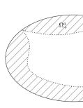
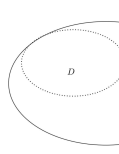
(i)                                                     (ii)

Figure 1: (i) An example where $(A.2)$ holds; (ii) An example where $(A.3)$ holds.

We start by showing that $(P_{\alpha})$ inherits the positivity property from the Dirichlet problem (i.e. for $q\in\mathcal{A}_{D}$) up to a certain $\alpha_{p}(a)>0$:

Theorem 1.2 (Positivity).

Assume $(A.1)$. Then there exists $\alpha_{p}=\alpha_{p}(a)>0$ such that any nontrivial solution of $(P_{\alpha})$ belongs to $\mathcal{P}^{\circ}$ for every $\alpha<\alpha_{p}$ and $q\in\mathcal{A}_{D}$. Moreover, $\alpha_{p}=\infty$ if $(A.2)$ holds.

In view of the above theorem, we shall deal with $q\in\mathcal{A}_{D}$ in most of our results. We proceed with the description of the solution set of $(P_{\alpha})$ for $\alpha<0$. This case turns out to be similar to the Dirichlet one, as long as existence and uniqueness of a nontrivial solution are concerned. As a matter of fact, when $\alpha<0$ we shall see that $(A.0)$ is not necessary for the existence of a positive solution, unlike in the case $\alpha\geq 0$ (for the Neumann problem see [6, Lemma 2.1], which can be easily extended to $\alpha>0$).

Theorem 1.3 (A curve of positive solutions for $\alpha<0$).

Assume $(A.1)$ and $q\in\mathcal{A}_{D}$. Then $(P_{\alpha})$ has a unique nontrivial solution $u_{\alpha}$ for each $\alpha<0$, and $u_{\alpha}\in\mathcal{P}^{\circ}$. Moreover, the mapping $\mathcal{C}_{0}:\alpha\mapsto u_{\alpha}$ is $C^{\infty}$ from $(-\infty,0)$ into $W^{2,r}(\Omega)$, increasing (i.e. $u_{\alpha}<u_{\beta}$ on $\overline{\Omega}$ for $\alpha<\beta<0$), and $u_{\alpha}\rightarrow u_{D}$ in $H^{1}(\Omega)$ as $\alpha\rightarrow-\infty$. Finally, as $\alpha\rightarrow 0^{-}$ we have the following alternative:

1. Assume that $\left(A.0\right)$ does not hold. Then $\displaystyle\min_{x\in\overline{\Omega}}u_{\alpha}(x)\rightarrow\infty$ as $\alpha\rightarrow 0^{-}$ (see Figure 2(i)). In particular, $u_{\alpha}$ approaches a spatially homogeneous distribution on $\overline{\Omega}$. Moreover, $(P_{\alpha})$ has no solution $u$ such that $u\not\equiv 0$ in $\Omega_{+}^{a}$ for $\alpha\geq 0$.

2. Assume that $\left(A.0\right)$ holds. Then $\mathcal{C}_{0}$ can be extended to $(-\infty,\overline{\alpha})$, for some $\overline{\alpha}>0$, so that $u_{0}=u_{N}$ and $u_{\alpha}\in\mathcal{P}^{\circ}$ solves $(P_{\alpha})$ for $\alpha\in(0,\overline{\alpha})$. Moreover, the mapping $\alpha\mapsto u_{\alpha}$ is increasing in $(-\infty,\overline{\alpha})$ and unique in the following sense: if $u_{n}$ solves $(P_{\alpha_{n}})$ with $\alpha_{n}\rightarrow 0^{+}$ and $u_{n}\rightarrow u_{N}$ in $C^{1}(\overline{\Omega})$, then, for $n$ large enough, $u_{n}=u_{\alpha}$ for some $\alpha\in(0,\overline{\alpha})$ (see Figure 2(ii)).

Remark 1.4.

1. Let $0<q<1$. Under $(A.1)$ there exists $\delta=\delta(q,a^{+})>0$ such that any nontrivial solution of $(P_{-\infty})$ lies in $\mathcal{P}^{\circ}$ if $0<\|a^{-}\|_{C(\overline{\Omega})}<\delta$, cf. [17, Theorem 1.1]. One may easily see from its proof that Theorem 1.3 also holds if we assume $0<\|a^{-}\|_{C(\overline{\Omega})}<\delta$, instead of $q\in\mathcal{A}_{D}$.

2. A ’bifurcation from infinity’ scenario as in Theorem 1.3(i) also occurs under $(A.0)$, now with $\alpha\rightarrow 0^{+}$ (see Theorem 1.5(ii-c)).

   

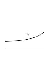
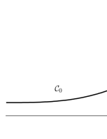
(i)                                            (ii)

Figure 2: The positive solutions curve $\mathcal{C}_{0}$ for $q\in\mathcal{A}_{D}$ in the cases (i) $\int_{\Omega}a\geq 0$ and (ii) $\int_{\Omega}a<0$.

Differently from the case $\alpha\leq 0$, we shall see that when $\alpha>0$ is small enough $(P_{\alpha})$ may admit multiple solutions in $\mathcal{P}^{\circ}$. To this end, we set

$$w:=\alpha^{\frac{1}{1-q}}u$$ (1.1)

and transform $(P_{\alpha})$ into

$$\begin{cases}-\Delta w=\alpha a(x)w^{q}&\mbox{in $\Omega$},\\ w\geq 0&\mbox{in $\Omega$},\\ \partial_{\nu}w=\alpha w&\mbox{on $\partial\Omega$}.\end{cases}$$

We shall treat this problem via a bifurcation approach, looking at $\alpha$ as a bifurcation parameter. It turns out that $(R_{\alpha})$ is easier to handle (in comparison with $(P_{\alpha})$), providing us with a more accurate description of the solutions set of $(P_{\alpha})$ for $\alpha>0$ small. Indeed, note that $(R_{\alpha})$ has two solutions lines, namely:

$$\begin{cases}\Gamma_{0}:=\{(\alpha,w):\alpha>0,\ w=0\},&\\ \Gamma_{1}:=\{(\alpha,w):\alpha=0,\ \mbox{$w$ is a nonnegative constant}\}.&\end{cases}$$ (1.2)

Under $(A.0)$, let us put

$$c_{a}:=\left(\frac{-\int_{\Omega}a}{|\partial\Omega|}\right)^{\frac{1}{1-q}}.$$ (1.3)

In [10, Section 7] Chabrowski and Tintarev proved, by variational methods, that under $(A.0)$ this problem has at least two nontrivial solutions $w_{1,\alpha},w_{2,\alpha}$ such that $w_{1,\alpha}<w_{2,\alpha}$ on $\overline{\Omega}$ for $\alpha>0$ small enough. Moreover, they also provided the following asymptotic profiles of $w_{1,\alpha},w_{2,\alpha}$ as $\alpha\rightarrow 0^{+}$:

$$w_{2,\alpha}\rightarrow c_{a}\quad\mbox{and}\quad w_{1,\alpha}\rightarrow 0\ \mbox{in}\ H^{1}(\Omega)\quad\mbox{as}\quad\alpha\rightarrow 0^{+},$$ (1.4)

and every sequence $\alpha_{n}\rightarrow 0$ has a subsequence (still denoted by the same notation) satisfying

$$\alpha_{n}^{-\frac{1}{1-q}}w_{1,\alpha_{n}}\rightarrow u_{0}\mbox{ in $H^{1}(\Omega)$},$$ (1.5)

where $u_{0}$ is a nontrivial solution of $(P_{0})$.

We shall complement (1.4) and (1.5) in two ways, proving the following:

• an exact multiplicity result for $q\in\mathcal{A}_{N}$, namely: $w_{1,\alpha},w_{2,\alpha}$ are the only nontrivial solutions of $(R_{\alpha})$ if $\alpha>0$ is small enough, and $w_{1,\alpha},w_{2,\alpha}\in\mathcal{P}^{\circ}$ (Theorem 3.14);

• the existence of a subcontinuum of solutions of $(R_{\alpha})$ for $\alpha>0$ small, connecting $(0,0)$ to $(0,c_{a})$ (Theorem 4.4, see also Remark 4.5).

These results, combined with Theorems 1.2 and 1.3, provide a global description (with respect to $\alpha$) of the solutions set of $(P_{\alpha})$ for $q\in\mathcal{A}_{D}$:

Theorem 1.5.

Assume $(A.0),(A.1)$, and $q\in\mathcal{A}_{D}$. Then the following assertions hold:

1. (Existence and nonexistence) Let

   $$\alpha_{s}:=\sup\{\alpha\in\mathbb{R}:\mbox{$(P_{\alpha})$ has a solution in $\mathcal{P}^{\circ}$}\}.$$ (1.6)

   Then $\alpha_{s}\in\left(0,\infty\right)$, i.e. $(P_{\alpha})$ has at least one solution in $\mathcal{P}^{\circ}$ for $\alpha>0$ small and no such solution for $\alpha>0$ large. In addition, if $(A.2)$ holds then $(P_{\alpha})$ has at least one solution in $\mathcal{P}^{\circ}$ for every $\alpha\leq\alpha_{s}$.

2. (Exact multiplicity and limiting behavior) There exists $\overline{\alpha}\in(0,\alpha_{s}]$ such that $(P_{\alpha})$ has exactly one nontrivial solution $u_{1,\alpha}$ for $\alpha\in(-\infty,0]$, and exactly two nontrivial solutions $u_{1,\alpha},u_{2,\alpha}$ for $\alpha\in(0,\overline{\alpha})$. Moreover $u_{1,\alpha},u_{2,\alpha}\in\mathcal{P}^{\circ}$ and these ones satisfy (see Figure 3(i)):

   1. $\mathcal{C}_{0}:\alpha\mapsto u_{1,\alpha}$ is a $C^{\infty}$ increasing mapping from $(-\infty,\overline{\alpha})$ into $W^{2,r}(\Omega)$ (as in Theorem 1.3(ii)), and $\mathcal{C}_{1}:\alpha\mapsto u_{2,\alpha}$ is a $C^{\infty}$ mapping from $(0,\overline{\alpha})$ into $W^{2,r}(\Omega)$.

   2. $u_{1,\alpha}\rightarrow u_{D}$ in $H^{1}(\Omega)$ as $\alpha\rightarrow-\infty$.

   3. $u_{2,\alpha}\sim\alpha^{-\frac{1}{1-q}}c_{a}$ as $\alpha\rightarrow 0^{+}$, i.e. $\alpha^{\frac{1}{1-q}}u_{2,\alpha}\rightarrow c_{a}$ in $C^{1}(\overline{\Omega})$ (implying $\displaystyle\min_{\overline{\Omega}}u_{2,\alpha}\rightarrow\infty$) as $\alpha\rightarrow 0^{+}$, where $c_{a}$ is given by (1.3).

3. (Existence of a component) Assume in addition $(A.2)$ and $\left(A.3\right)$. Then $(P_{\alpha})$ possesses a component $\mathcal{C}_{\ast}$ (i.e. a maximal closed, connected subset in $\mathbb{R}\times C^{1}(\overline{\Omega})$) of solutions in $\mathcal{P}^{\circ}$ that contains $\mathcal{C}_{0}$ and $\mathcal{C}_{1}$. In addition,

   $$\mathcal{C}_{\ast}\cap\left\{(\alpha,0):\alpha\in\mathbb{R}\right\}=\emptyset,$$

   and

   $$\mathcal{C}_{\ast}\cap\{(\alpha,\infty):\alpha\in\mathbb{R}\}=\{(0,\infty)\},$$

   i.e. $\mathcal{C}_{\ast}$ does not meet the trivial solution at any $\alpha\in\mathbb{R}$ and $\mathcal{C}_{\ast}$ bifurcates from infinity only at $\alpha=0$, see Figure 3(ii).

   

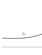
(i)                                            (ii)

Figure 3: (i) The $C^{\infty}$ curves $\mathcal{C}_{0}$ and $\mathcal{C}_{1}$, (ii) The component $\mathcal{C}_{\ast}$.

Remark 1.6.

1. One may easily check that all the assertions for $\alpha\geq 0$ in Theorem 1.5 still hold if we take $q\in\mathcal{A}_{N}$ in place of $q\in\mathcal{A}_{D}$ (let us note that $\mathcal{A}_{N}\supseteq\mathcal{A}_{D}$ by Proposition 2.3 below).

2. Some lower and upper bounds on $\alpha_{s}$ are given in Corollary 3.8. Moreover, we shall provide (finite) upper bounds for $\alpha_{s}$ for every $q\in[0,1)$, see Proposition 3.6 below.

3. The approach to obtain the solution $u_{2,\alpha}$ from Theorem 1.5(ii) applies to any $q\in[0,1)$. Thus, for $q$ close to $0$ (including $q=0$), $(P_{\alpha})$ still has, under $(A.0)$, a solution in $\mathcal{P}^{\circ}$ for $\alpha>0$ small, see Remark 3.12. We note that when $q=0$ and $\int_{\Omega}a<0$ there are no solutions of $\left(P_{\alpha}\right)$ in $\mathcal{P}^{\circ}$ for $\alpha\in\left[-\infty,0\right]$, since in this case solutions $u$ satisfy $-\int_{\Omega}a=\alpha\int_{\partial\Omega}u$ if $\alpha\neq-\infty$ and $-\int_{\Omega}a=\int_{\partial\Omega}\partial_{\nu}u$ if $\alpha=-\infty$.

4. Theorems 1.2, 1.3 and 1.5 hold more generally for $a\in L^{r}(\Omega)$, with $r>N$. In this case, we set $\Omega_{+}^{a}$ as the largest open subset of $\Omega$ in which $a>0$ a.e., and we add to $(A.1)$ the condition $|(\text{supp}\,a^{+})\setminus\Omega_{+}^{a}|=0$, where supp is the support in the measurable sense.

To the best of our knowledge, exact multiplicity results are not commonly seen in the literature, specially for indefinite type problems such as $(P_{\alpha})$. We refer to [20, Section 3] for a result of this kind with $N=1$ and a superlinear nonlinearity. Let us add that some multiplicity results for $(P_{-\infty})$ and $(P_{0})$ are given in [5, Section 2] and [6, Section 4], [1, Theorem 1.1] respectively.

Finally, although we are mainly focused on $q\in(0,1)$, we shall see that when $q=0$ and $\alpha>0$ many interesting questions arise. Some of them are treated in this article, whereas some other ones are left to a forthcoming paper.

The rest of the article is organized as follows. In Section 2 we mainly analyze the case $\alpha\leq 0$ and prove Theorems 1.2 and 1.3. Section 3 is mostly devoted to $(R_{\alpha})$ with $\alpha>0$, where we investigate qualitative properties of the solutions set and prove an exact multiplicity result employing the change of variables (1.1). Lastly, Section 4 provides a topological bifurcation approach of $(R_{\alpha})$ and the proof of Theorem 1.5.

Notation

• For any $f\in L^{1}(\Omega)$ the integral $\int_{\Omega}f$ is considered with respect to the Lebesgue measure, whereas for any $g\in L^{1}(\partial\Omega)$ the integral $\int_{\partial\Omega}g$ is considered with respect to the surface measure.

• The usual norm of $H^{1}(\Omega)$ is denoted by $\|\cdot\|$, i.e. $\|u\|=\left(\int_{\Omega}|\nabla u|^{2}+u^{2}\right)^{\frac{1}{2}}$. For $r\geq 1$ the Lebesgue norm in $L^{r}(\Omega)$ will be denoted by $\|\cdot\|_{r}$.

• The weak convergence is denoted by $\rightharpoonup$.

• The positive and negative parts of a function $u$ are defined by $u^{\pm}:=\max\{\pm u,0\}$.

• $|\cdot|$ stands for both the Lebesgue measure and the surface measure.

• The characteristic function of a set $A\subset\mathbb{R}^{N}$ is denoted by $\chi_{A}$.

2 Proof of Theorems 1.2 and 1.3

We split the proofs of Theorems 1.2 and 1.3 into several results. The first one is a direct consequence of Lemma 2.1 and Proposition 2.3, whereas the second one follows from Propositions 2.4, 2.6 and 2.7.

We start by proving that nontrivial solutions of $(P_{\alpha})$ are positive in some component of $\Omega^{a}_{+}$ as long as $\alpha$ is less than

$$\alpha_{p}=\alpha_{p}(a):=\inf\left\{\int_{\Omega}|\nabla v|^{2}:v\in H^{1}(\Omega),v\equiv 0\text{ in }\Omega^{a}_{+},\int_{\partial\Omega}v^{2}=1\right\}.$$

Note that $\alpha_{p}$ depends on $a$ but not on $q$.

Lemma 2.1.

1. We have $\alpha_{p}>0$. Moreover $\alpha_{p}=\infty$ if, and only if, $(A.2)$ holds.

2. We have $u\not\equiv 0$ in $\Omega_{+}^{a}$ for any nontrivial solution $u$ of $(P_{\alpha})$ and for any $\alpha<\alpha_{p}$ and $q\in[0,1)$.

Proof.

1. First of all, one may easily show that this infimum is achieved whenever it is finite, and consequently that it is positive, since no constant function satisfies the constraints simultaneously. Now, if $(A.2)$ holds then there is no $v$ satisfying $v\equiv 0$ in $\Omega_{a}^{+}$ and $\int_{\partial\Omega}v^{2}=1$, so that $\alpha_{p}=\infty$. Finally, if $(A.2)$ does not hold then we may find some ball $B$ around some $x_{0}\in\partial\Omega$ such that $a\leq 0$ in $B\cap\Omega$. We may then build some $v\in H^{1}(\Omega)$ supported in $B\cap\Omega$ and such that $\int_{\partial\Omega}v^{2}=1$. Thus $v$ is admissible for $\alpha_{p}$, and consequently $\alpha_{p}<\infty$.

2. Let $\alpha<\alpha_{p}$ and $u$ be a nontrivial solution of $(P_{\alpha})$. If $u\equiv 0$ in $\Omega_{a}^{+}$ then we have

   $$0<\int_{\Omega}|\nabla u|^{2}=\int_{\Omega}a(x)u^{q+1}+\alpha\int_{\partial\Omega}u^{2}\leq\alpha\int_{\partial\Omega}u^{2},$$

   so that $\alpha\geq(\int_{\Omega}|\nabla u|^{2})(\int_{\partial\Omega}u^{2})^{-1}$. Consequently $\alpha\geq\alpha_{p}$, which contradicts our assumption. ∎
   

Remark 2.2.

Assume that $\Omega_{0,+}^{a}:=\{x\in\Omega:a(x)\geq 0\}$ is connected and smooth. Then $\alpha_{p}$ can be reset as

$$\alpha_{p}=\alpha_{p}(a):=\inf\left\{\int_{\Omega}|\nabla v|^{2}:v\in H^{1}(\Omega),v\equiv 0\text{ on }\Omega_{0,+}^{a},\int_{\partial\Omega}v^{2}=1\right\}.$$

In this case, Lemma 2.1(i) holds with $(A.2)$ formulated now as $\partial\Omega\subseteq\partial\Omega_{0,+}^{a}$. Moreover, one can repeat the proof of Lemma 2.1(ii) to show that $u\not\equiv 0$ on $\Omega^{a}_{0,+}$ for any nontrivial solution $u$ of $(P_{\alpha})$ and any $\alpha<\alpha_{p}$. Since $\Omega_{0,+}^{a}$ is smooth and connected, the strong maximum principle yields $u>0$ in $\Omega_{+}^{a}$. Note that this new value $\alpha_{p}$ is larger than the original one.

Proposition 2.3 (Monotonicity of $\mathcal{A}_{\alpha}$).

We have $\mathcal{A}_{\alpha}\subseteq\mathcal{A}_{\beta}$ for $-\infty\leq\alpha<\beta<\alpha_{p}$.

Proof. First we consider $\alpha=-\infty$. Let $q\in\mathcal{A}_{D}$ and $u$ be a nontrivial solution of $(P_{\beta})$. Since $u\geq 0$ on $\overline{\Omega}$, we see that $u$ is a supersolution of $(P_{-\infty})$. Moreover, by Lemma 2.1 we know that $u\not\equiv 0$ in $\Omega_{+}^{a}$. It follows that there exist a ball $B\subset\Omega_{+}^{a}$ and a constant $c>0$ such that $u>c$ in $B$. It is then possible to provide a subsolution $z$ of $(P_{-\infty})$ such that $z\not\equiv 0$, $\mathrm{supp\,}z\Subset B$, and $z\leq u$ (see e.g. the construction in [5, Lemma 2.3(ii)]). By the sub and supersolution method, we find a nontrivial solution $u_{1}$ of $(P_{-\infty})$ such that $z\leq u_{1}\leq u$ on $\overline{\Omega}$. Since $q\in\mathcal{A}_{D}$, we have $u_{1}\in\mathcal{P}^{\circ}$, so $u\geq u_{1}>0$ in $\Omega$ and $\partial_{\nu}u_{1}<0$ on $\partial\Omega$. We claim that $u>0$ on $\partial\Omega$. Indeed, otherwise we have $u=\partial_{\nu}u=0$ somewhere on $\partial\Omega$. But since $u_{1}=0>\partial_{\nu}u_{1}$ on $\partial\Omega$, this contradicts the assertion $u_{1}\leq u$ in $\Omega$. Hence $u>0$ on $\overline{\Omega}$, which shows that $q\in\mathcal{A}_{\beta}$.

Let now $\alpha>-\infty$. Take $q\in\mathcal{A}_{\alpha}$ and $u$ a nontrivial solution of $(P_{\beta})$. Then, arguing as in the previous case, we find by the sub and supersolution method a nontrivial solution $u_{1}$ of $(P_{\alpha})$ such that $u_{1}\leq u$ on $\overline{\Omega}$. Since $q\in\mathcal{A}_{\alpha}$, it follows that $u\geq u_{1}>0$ on $\overline{\Omega}$, which shows that $q\in\mathcal{A}_{\beta}$. ∎

Next we deal with

$$\tilde{\alpha}=\tilde{\alpha}(q,a):=\inf\left\{\int_{\Omega}|\nabla v|^{2}:v\in H^{1}(\Omega),\int_{\Omega}a(x)|v|^{q+1}\geq 0,\int_{\partial\Omega}v^{2}=1\right\}.$$ (2.1)

One may easily show that this infimum is achieved. Note also that $\tilde{\alpha}\geq 0$ and that $\tilde{\alpha}>0$ if, and only if, $(A.0)$ holds. Lastly, one may show that $\displaystyle\liminf_{q\to 1^{-}}\tilde{\alpha}(q,a)\geq\tilde{\alpha}(1,a)$, so that $\tilde{\alpha}(q,a)$ stays away from zero for $q$ close to $1$ if $(A.0)$ holds.

Proposition 2.4 (Existence of a solution in $\mathcal{P}^{\circ}$).

$(P_{\alpha})$ has at least one solution $u_{\alpha}$ such that $u_{\alpha}\not\equiv 0$ in $\Omega_{a}^{+}$ for every $\alpha<\tilde{\alpha}$. In addition:

1. Assume $(A.1)$ and $q\in\mathcal{A}_{D}$. Then $u_{\alpha}\in\mathcal{P}^{\circ}$ and $u_{\alpha}$ is the unique nontrivial solution of $(P_{\alpha})$ for $\alpha<0$.

2. Assume $(A.0)$, $(A.1)$ and $q\in\mathcal{A}_{N}$. Then $u_{\alpha}\in\mathcal{P}^{\circ}$ for $0<\alpha<\tilde{\alpha}$.

Proof. Let

$$\mu(\alpha):=\inf\left\{\int_{\Omega}|\nabla u|^{2}-\alpha\int_{\partial\Omega}u^{2}:u\in H^{1}(\Omega),\int_{\Omega}a(x)|u|^{q+1}=1\right\}$$ (2.2)

We claim that $\mu(\alpha)$ is finite if $\alpha<\tilde{\alpha}$. Indeed, assume by contradiction that $u_{n}$ satisfies $\int_{\Omega}a(x)|u_{n}|^{q+1}=1$ and $\int_{\Omega}|\nabla u_{n}|^{2}-\alpha\int_{\partial\Omega}u_{n}^{2}\rightarrow-\infty$. In particular, we have $\|u_{n}\|\rightarrow\infty$. We set $v_{n}:=\frac{u_{n}}{\|u_{n}\|}$ and assume that $v_{n}\rightharpoonup v_{0}$ in $H^{1}(\Omega)$, $v_{n}\rightarrow v_{0}$ in $L^{t}(\Omega)$ for $1\leq t<2^{\ast}$ and in $L^{2}(\partial\Omega)$, and $v_{n}\rightarrow v_{0}$ a.e. in $\Omega$, for some $v_{0}\in H^{1}(\Omega)$. Then

$$\int_{\Omega}|\nabla v_{0}|^{2}-\alpha\int_{\partial\Omega}v_{0}^{2}\leq\liminf\left(\int_{\Omega}|\nabla v_{n}|^{2}-\alpha\int_{\partial\Omega}v_{n}^{2}\right)\leq 0$$

and $\int_{\Omega}a(x)|v_{n}|^{q+1}=\|u_{n}\|^{-(q+1)}\rightarrow 0$. Hence $\int_{\Omega}a(x)|v_{0}|^{q+1}=0$. Moreover, $v_{0}\not\equiv 0$ since otherwise, from the above inequality, we would have $v_{n}\rightarrow 0$ in $H^{1}(\Omega)$, which is impossible. Thus we have $\alpha\geq\frac{\int_{\Omega}|\nabla v_{0}|^{2}}{\int_{\partial\Omega}v_{0}^{2}}$, which contradicts $\alpha<\tilde{\alpha}$. Therefore $\mu(\alpha)$ is finite, and repeating the above argument we can show that it is achieved by some nonnegative $u$. By the Lagrange multipliers rule, we find that $u$ satisfies $-\Delta u=\mu(\alpha)a(x)u^{q}$ in $\Omega$ and $\partial_{\nu}u=\alpha u$ on $\partial\Omega$. Note that since $\alpha<\tilde{\alpha}$ we have $\mu(\alpha)>0$. We set $u_{\alpha}:=\mu(\alpha)^{-\frac{1}{1-q}}u$ to get a solution of $(P_{\alpha})$ such that $\int_{\Omega}a(x)u_{\alpha}^{q+1}>0$, so that $u_{\alpha}\not\equiv 0$ in $\Omega_{a}^{+}$. Now, if $q\in\mathcal{A}_{D}$ then, from Proposition 2.3 it follows that $q\in\mathcal{A}_{\alpha}$ for every $\alpha<0$, so that $u_{\alpha}\in\mathcal{P}^{\circ}$. Since $(P_{\alpha})$ has at most one solution in $\mathcal{P}^{\circ}$ for each $\alpha<0$ (see Theorem 1.1(iii)), we infer that $u_{\alpha}$ is the unique nontrivial solution of $(P_{\alpha})$.

Finally, assume $(A.0)$ and $q\in\mathcal{A}_{N}$. Then, for $0<\alpha<\tilde{\alpha}$ we have that $u_{\alpha}$ is a supersolution of $\left(P_{0}\right)$. Thus, since it is easy to provide small nontrivial subsolutions of $\left(P_{0}\right)$ (see e.g. the construction in [5, Lemma 2.3(ii)]), recalling Theorem 1.1(v) we deduce that $u_{\alpha}\geq u_{N}$ on $\overline{\Omega}$, and we get the desired conclusion. ∎

Next, for $\alpha\leq 0$ and $u=u_{\alpha}$, we consider the eigenvalue problem

$$\begin{cases}-\Delta\phi=a(x)qu^{q-1}\phi+\gamma\phi&\mbox{in $\Omega$},\\ \partial_{\nu}\phi=\alpha\phi&\mbox{on $\partial\Omega$},\end{cases}$$

where $\gamma=\gamma(\alpha,u)$ is an eigenvalue parameter. It is well known that this problem has a smallest eigenvalue $\gamma_{1}=\gamma_{1}(\alpha,u)$, which is simple and possesses an eigenfunction $\phi_{1}\in\mathcal{P}^{\circ}$.

Lemma 2.5 (Non-degeneracy).

Whenever $u_{\alpha}$ exists for $\alpha\leq 0$, we have $\gamma_{1}(\alpha,u_{\alpha})>0$.

Proof. By a direct computation and using Green’s formula we infer that

$$\gamma_{1}\int_{\Omega}u^{q}\phi_{1} =\int_{\Omega}\left(-\Delta\phi_{1}\cdot u^{q}+\Delta u\cdot qu^{q-1}\phi_{1}\right)$$

$$=\int_{\Omega}\nabla\phi_{1}\cdot\nabla(u^{q})-\nabla u\cdot\nabla\left(qu^{q-1}\phi_{1}\right)+\int_{\partial\Omega}qu^{q-1}\phi_{1}\partial_{\nu}u-u^{q}\partial_{\nu}\phi_{1}$$

$$=q(1-q)\int_{\Omega}u^{q-2}|\nabla u|^{2}\phi_{1}-\alpha(1-q)\int_{\partial\Omega}u^{q}\phi_{1},$$

and the conclusion follows. ∎

Proposition 2.6 (Existence of an increasing curve).

Assume $(A.1)$ and $q\in\mathcal{A}_{D}$. Then $\alpha\mapsto u_{\alpha}$ is $C^{\infty}$ from $(-\infty,0)$ into $W^{2,r}(\Omega)$ and $u_{\alpha}<u_{\beta}$ on $\overline{\Omega}$ for $\alpha<\beta<0$. Moreover $u_{\alpha}\rightarrow u_{D}$ in $H^{1}(\Omega)$ as $\alpha\rightarrow-\infty$.

Proof. Based on Lemma 2.5, we show that $\alpha\mapsto u_{\alpha}$ is $C^{\infty}$ from $(-\infty,0)$ into $W^{2,r}(\Omega)$. Let $\delta>0$ and $B_{0}$ be a small open ball in $W^{2,r}(\Omega)$ with center $u_{\alpha}$, so that $B_{0}\subset\mathcal{P}^{\circ}$. Set

$$\mathcal{F}: (\alpha-\delta,\alpha+\delta)\times B_{0}\longrightarrow L^{r}(\Omega)\times W^{1-\frac{1}{r},r}(\partial\Omega)$$

$$\qquad(\beta,u)\longmapsto\left(-\Delta u-a(x)u^{q},\;\partial_{\nu}u-\beta u\right).$$

We see that $\mathcal{F}(\alpha,u_{\alpha})=0$, and the Fréchet derivative $\mathcal{F}_{u}(\beta,u):W^{2,r}(\Omega)\rightarrow L^{r}(\Omega)\times W^{1-\frac{1}{r},r}(\partial\Omega)$ is given by $\mathcal{F}_{u}(\beta,u)\varphi=\left(-\Delta\varphi-a(x)qu^{q-1}\varphi,\partial_{\nu}\varphi-\beta\varphi\right)$. From Lemma 2.5 we infer that $\mathcal{F}_{u}(\alpha,u_{\alpha})$ is a homeomorphism, using the index theory for Fredholm operators, and thus, the desired assertion follows by the implicit function theorem.

We may then differentiate $(P_{\alpha})$ with respect to $\alpha$ to obtain

$$\begin{cases}-\Delta u_{\alpha}^{\prime}=qa(x)u_{\alpha}^{q-1}u_{\alpha}^{\prime}&\mbox{in $\Omega$},\\ \partial_{\nu}u_{\alpha}^{\prime}=u_{\alpha}+\alpha u_{\alpha}^{\prime}&\mbox{on $\partial\Omega$}.\end{cases}$$

Set $\mathcal{L}:=-\Delta-qa(x)u_{\alpha}^{q-1}$ and $\mathcal{B}:=\frac{\partial}{\partial\nu}-\alpha$. It follows that

$$\begin{cases}\mathcal{L}u_{\alpha}^{\prime}=0&\mbox{in $\Omega$},\\ \mathcal{B}u_{\alpha}^{\prime}=u_{\alpha}>0&\mbox{on $\partial\Omega$}.\end{cases}$$

Lemma 2.5 enables us to apply [24, Theorem 7.10] to deduce that $u_{\alpha}^{\prime}\in\mathcal{P}^{\circ}$ for every $\alpha<0$, which shows that $u_{\alpha}$ is increasing with respect to $\alpha$.

Let now $\alpha_{n}\rightarrow-\infty$ and $u_{n}:=u_{\alpha_{n}}$. We may assume that $\alpha_{n}$ is decreasing, and so is $u_{n}$. Thus $\|u_{n}\|_{C(\overline{\Omega})}$ is clearly bounded, and since $u_{n}$ is a solution of $(P_{\alpha_{n}})$, we deduce that $\|u_{n}\|$ is bounded. Hence, up to a subsequence, $u_{n}\rightharpoonup u_{\infty}$ in $H^{1}(\Omega)$, $u_{n}\rightarrow u_{\infty}$ in $L^{t}(\Omega)$ for $1\leq t<2^{\ast}$, and in $L^{2}(\partial\Omega)$, and $u_{n}\rightarrow u_{\infty}$ a.e. in $\Omega$, for some $u_{\infty}\in H^{1}(\Omega)$. In particular, $u_{\infty}$ is nonnegative. Since $u_{n}$ is a solution of $(P_{\alpha_{n}})$, we obtain

$$-\alpha_{n}\int_{\partial\Omega}u_{n}=\int_{\Omega}a(x)u_{n}^{q}\leq C\|u_{n}\|_{C(\overline{\Omega})}^{q}\leq C^{\prime}.$$

As $-\alpha_{n}\rightarrow\infty$, it follows that $\int_{\partial\Omega}u_{n}\rightarrow\int_{\partial\Omega}u_{\infty}=0$, so that $u_{\infty}=0$ on $\partial\Omega$, implying $u_{\infty}\in H_{0}^{1}(\Omega)$. Using the different convergences of $u_{n}$ towards $u_{0}$ and standard arguments, we find that $u_{n}\rightarrow u_{\infty}$ in $H^{1}(\Omega)$. From the weak formulation of $(P_{\alpha})$ we deduce that $u_{\infty}$ is a weak solution of $(P_{-\infty})$. Finally, note from (2.2) that $\mu(\alpha)\leq\int_{\Omega}|\nabla v|^{2}$ for any $v\in H_{0}^{1}(\Omega)$ such that $\int_{\Omega}a(x)|v|^{q+1}=1$. Hence $\mu(\alpha)\leq C$ for some constant $C>0$ and any $\alpha$. It follows that $\int_{\Omega}a(x)u_{n}^{q+1}=\mu(\alpha_{n})^{-\frac{q+1}{1-q}}\geq C^{-\frac{q+1}{1-q}}>0$ for every $n$, which implies that $u_{\infty}$ is nontrivial. Since $q\in\mathcal{A}_{D}$ we have $u_{\infty}=u_{D}$, as desired. ∎

Proposition 2.7 (Asymptotic behavior as $\alpha\to 0^{-}$).

Assume $(A.1)$ and $q\in\mathcal{A}_{D}$.

1. If $\int_{\Omega}a\geq 0$ then $\displaystyle\min_{x\in\overline{\Omega}}u_{\alpha}(x)\rightarrow\infty$ as $\alpha\rightarrow 0^{-}$, and $(P_{\alpha})$ has no solution $u$ such that $u\not\equiv 0$ in $\Omega_{+}^{a}$ for $\alpha\geq 0$ (in particular it has no nontrivial solution for $0\leq\alpha<\alpha_{p}$).

2. If $\int_{\Omega}a<0$ then the curve $\alpha\mapsto u_{\alpha}$ can be extended to $(-\infty,\overline{\alpha})$, for some $\overline{\alpha}>0$, so that $u_{0}=u_{N}$ and $u_{\alpha}\in\mathcal{P}^{\circ}$ is a solution of $(P_{\alpha})$ for $\alpha\in(0,\overline{\alpha})$. Moreover, $\alpha\mapsto u_{\alpha}$ is increasing in $(-\infty,\overline{\alpha})$, and unique in the following sense: if $u_{n}$ is a solution of $(P_{\alpha_{n}})$ such that $\alpha_{n}\rightarrow 0^{+}$ and $u_{n}\rightarrow u_{N}$ in $C^{1}(\overline{\Omega})$, then, for $n$ large enough, $u_{n}=u_{\alpha}$ for some $\alpha\in(0,\overline{\alpha})$.

Proof.

1. First we prove $\|u_{\alpha}\|_{C(\overline{\Omega})}\rightarrow\infty$ as $\alpha\rightarrow 0^{-}$. Since $u_{\alpha}\in\mathcal{P}^{\circ}$ is a solution of $(P_{\alpha})$, it suffices to show $\|u_{\alpha}\|\rightarrow\infty$ as $\alpha\rightarrow 0^{-}$. Assume by contradiction that for some sequence $\alpha_{n}\rightarrow 0^{-}$, $\|u_{\alpha_{n}}\|$ is bounded. By elliptic regularity, it follows that, up to a subsequence, $u_{\alpha_{n}}\rightarrow u_{\ast}$ in $C^{1}(\overline{\Omega})$ for some $u_{\ast}$. By definition, we deduce that $u_{\ast}$ is a solution of $(P_{0})$. Moreover, $u_{\ast}\in\mathcal{P}^{\circ}$ by the monotonicity of $u_{\alpha_{n}}$, i.e. $u_{\ast}=u_{N}$. However, this contradicts [6, Corollary 2.1] (which clearly holds in our setting), as desired.

   Now, by monotonicity it suffices to show the existence of a sequence $\alpha_{n}\rightarrow 0^{-}$ such that $\min_{\overline{\Omega}}u_{\alpha_{n}}\rightarrow\infty$. Let $\alpha_{n}\rightarrow 0^{-}$. Set $u_{n}:=u_{\alpha_{n}}$ and $v_{n}:=u_{n}/\|u_{n}\|_{C(\overline{\Omega})}$. Then it follows that

   $$\int_{\Omega}|\nabla v_{n}|^{2}\leq\left(\int_{\Omega}a(x)v_{n}^{q+1}\right)\|u_{n}\|_{C(\overline{\Omega})}^{q-1}\rightarrow 0.$$

   We deduce that, up to a subsequence, $v_{n}\rightarrow c_{\ast}$ in $H^{1}(\Omega)$, where $c_{\ast}$ is a nonnegative constant. Since $v_{n}$ satisfies

   $$\begin{cases}-\Delta v_{n}=a(x)\|u_{n}\|_{C(\overline{\Omega})}^{q-1}v_{n}^{q}&\mbox{in $\Omega$},\\ \partial_{\nu}v_{n}=\alpha_{n}v_{n}&\mbox{on $\partial\Omega$},\end{cases}$$

   we find that $\|v_{n}\|_{C^{\theta}(\overline{\Omega})}$ is bounded for $\theta\in(0,1)$ by elliptic regularity and a bootstrap argument [31, Theorem 2.2]. By a compactness argument, we infer that, up to a subsequence, $v_{n}\rightarrow c_{\ast}$ in $C(\overline{\Omega})$ and $c_{\ast}>0$, from which our desired conclusion follows.

   Finally, if $u$ is a nontrivial solution of $(P_{\alpha})$ such that $u\not\equiv 0$ in $\Omega_{+}^{a}$ and $\alpha\geq 0$ then $u$ is a supersolution of $(P_{0})$. Hence $(P_{0})$ has a nontrivial solution $u_{0}$, and since $q\in\mathcal{A}_{D}$, we have $u_{0}\in\mathcal{P}^{\circ}$. Reasoning as in [6, Lemma 2.1] we infer that $(A.0)$ holds, which contradicts our assumption.

2. From $(A.0)$ and $q\in\mathcal{A}_{N}$ (by Proposition 2.3), we know that $u_{N}\in\mathcal{P}^{\circ}$ is the unique nontrivial solution of $(P_{0})$. By Lemma 2.5 we have $\gamma_{1}(0,u_{N})>0$. Arguing as in the proof of Proposition 2.6, the implicit function theorem allows us to find some $\overline{\alpha}>0$ and an increasing $C^{\infty}$ curve $(\alpha,u_{\alpha})$ with $u_{\alpha}\in\mathcal{P}^{\circ}$ solutions of $(P_{\alpha})$, parametrized by $\alpha\in(-\overline{\alpha},\overline{\alpha})$. Lastly, let $u_{n}$ be a nontrivial solution of $(P_{\alpha_{n}})$ such that $\alpha_{n}\rightarrow 0^{+}$ and $u_{n}\rightarrow u_{0}$ in $C^{1}(\overline{\Omega})$. So, the Lebesgue dominated convergence theorem shows that

   $$\begin{cases}-\Delta(u_{n}-u_{0})=a(x)(u_{n}^{q}-u_{0}^{q})\rightarrow 0&\mbox{in $L^{r}(\Omega)$},\\ \partial_{\nu}(u_{n}-u_{0})+(u_{n}-u_{0})=\alpha_{n}u_{n}+(u_{n}-u_{0})\rightarrow 0&\mbox{in $C^{1}(\partial\Omega)$}.\end{cases}$$

   We deduce then, by elliptic regularity, that $u_{n}\rightarrow u_{0}$ in $W^{2,r}(\Omega)$. Combining the existence result with an application of the implicit function theorem provides the desired assertion. ∎
   

3 Qualitative analysis and exact multiplicity

In this section we prove an exact multiplicity result for $(R_{\alpha})$. Furthermore, we establish some preliminary results to prove Theorem 4.4 below, which states the existence of a subcontinuum $\gamma_{0}=\{(\alpha,w)\in[0,\infty)\times C^{1}(\overline{\Omega})\}$ of solutions of $(R_{\alpha})$ such that

$$\gamma_{0}\cap(\Gamma_{0}\cup\Gamma_{1})=\left\{(0,0),(0,c_{a})\right\}$$ (3.1)

(recall that $\Gamma_{0}$ and $\Gamma_{1}$ are the solution lines of $\left(R_{\alpha}\right)$ given by (1.2), see Figure 4). We shall use this result to prove Theorem 1.5(iii).

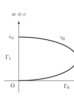
Figure 4: The bounded component $\gamma_{0}$ of nontrivial solutions of $(R_{\alpha})$ when $\int_{\Omega}a<0$.

First we show the existence of an a priori lower bound in $C(\overline{\Omega})$ for positive solutions of $(P_{\alpha})$ with $\alpha\in\mathbb{R}$, which shows that such solutions do not bifurcate from zero at any $\alpha\in\mathbb{R}$:

Lemma 3.1 (A priori lower bound).

There exists $C>0$ such that $\|u\|_{C(\overline{\Omega})}\geq C$ for every positive supersolution of $(P_{\alpha})$ and every $\alpha\in\mathbb{R}$. In particular, given $\beta>0$ there exists $C_{\beta}>0$ such that $\|w\|_{C(\overline{\Omega})}\geq C_{\beta}$ for every positive supersolution of $(R_{\alpha})$ with $\alpha\geq\beta$.

Proof. The first inequality is a direct consequence of [17, Lemma 2.2], and by the change of variables (1.1), we see that it implies the second one.∎

Second we discuss bifurcation from infinity at $\alpha\geq 0$. The following result asserts that $\alpha=0$ is the only point where solutions of $(R_{\alpha})$ bifurcate from infinity, and such solutions are given precisely by $\Gamma_{1}$.

Proposition 3.2 (Bifurcation from infinity and a priori upper bounds).

Given $\overline{\alpha}>0$, there exists $C_{\overline{\alpha}}>0$ such that $\|w\|_{C^{1}(\overline{\Omega})}\leq C_{\overline{\alpha}}$ for all solutions $w$ of $(R_{\alpha})$ with $0<\alpha<\overline{\alpha}$.

Proof. Assume by contradiction that there exist $(\alpha_{n},w_{n})$ such that $w_{n}$ is a solution of $(R_{\alpha_{n}})$, $\alpha_{n}\rightarrow\alpha_{0}\geq 0$, and $\|w_{n}\|_{C^{1}(\overline{\Omega})}\rightarrow\infty$. By elliptic regularity, it follows that $\|w_{n}\|\rightarrow\infty$. If we set $\psi_{n}:=w_{n}/\|w_{n}\|$ then we may assume that for some $\psi\in H^{1}(\Omega)$ and $1\leq t<2^{\ast}$,

$$\left\{\begin{array}[c]{l}\psi_{n}\rightharpoonup\psi\quad\mbox{in}\quad H^{1}(\Omega),\qquad\psi_{n}\rightarrow\psi\quad\mbox{in}\quad L^{t}(\Omega),\\ \psi_{n}\rightarrow\psi\quad\mbox{in}\quad L^{2}(\partial\Omega),\qquad\psi_{n}\rightarrow\psi\quad\mbox{a.e. in $\Omega$.}\end{array}\right.$$ (3.2)

Since $w_{n}$ is a weak solution of $(R_{\alpha_{n}})$, we see that

$$\int_{\Omega}\nabla w_{n}\nabla\varphi=\alpha_{n}\int_{\Omega}a\left(x\right)w_{n}^{\;q}\varphi+\alpha_{n}\int_{\partial\Omega}w_{n}\varphi,\quad\forall\varphi\in H^{1}(\Omega).$$

Dividing it by $\|w_{n}\|$, it follows that

$$\int_{\Omega}\nabla\psi_{n}\nabla\varphi=\alpha_{n}\left(\int_{\Omega}a(x)\psi_{n}^{\;q}\varphi\right)\|w_{n}\|^{q-1}+\alpha_{n}\int_{\partial\Omega}\psi_{n}\varphi,$$ (3.3)

so that $\int_{\Omega}\nabla\psi\nabla\varphi=\alpha_{0}\int_{\partial\Omega}\psi\varphi$ for all $\varphi\in H^{1}(\Omega)$. Hence $\psi\geq 0$ solves the problem

$$\begin{cases}\Delta\psi=0&\mbox{in $\Omega$},\\ \partial_{\nu}\psi=\alpha_{0}\psi&\mbox{on $\partial\Omega$},\end{cases}$$ (3.4)

Taking $\varphi\equiv 1$ in (3.3) we find that $\|w_{n}\|^{q-1}\int_{\Omega}a(x)\psi_{n}^{\;q}+\int_{\partial\Omega}\psi_{n}=0$. Passing to the limit, we have $\int_{\partial\Omega}\psi=0$, i.e. $\psi\equiv 0$ on $\partial\Omega$, so that $\psi\equiv 0$ from (3.4). Since $\|\psi_{n}\|=1$, we deduce that $\psi_{n}\rightharpoonup 0$ but $\psi_{n}\not\rightarrow 0$ in $H^{1}(\Omega)$.

Finally, taking $\varphi=\psi_{n}$ in (3.3) we find that

$$0=\int_{\Omega}|\nabla\psi|^{2}\leq\displaystyle\liminf_{n\rightarrow\infty}\int_{\Omega}|\nabla\psi_{n}|^{2}=\alpha_{0}\int_{\partial\Omega}\psi^{2}=0,$$

and thus that $\psi_{n}\rightarrow 0$ in $H^{1}(\Omega)$, a contradiction. ∎

Using Proposition 3.2 we show that (under the conditions of Theorem 1.5) the existence range for nontrivial solutions of $(P_{\alpha})$ is an interval. We set

$$\alpha_{s}:=\sup\{\alpha>0:\mbox{$(P_{\alpha})$ has a nontrivial solution}\}.$$

Note that this definition is equivalent to (1.6) if $(A.2)$ holds and $q\in\mathcal{A}_{N}$, in view of Lemma 2.1 and Proposition 2.3.

Proposition 3.3.

Assume $(A.1)$ and $(A.2)$. If $(P_{\alpha})$ has a nontrivial solution for some $\alpha>0$, then $(P_{\alpha})$ has at least one nontrivial solution for $0\leq\alpha\leq\alpha_{s}$ ($0\leq\alpha<\infty$ if $\alpha_{s}=\infty$).

Proof. We may assume that $\alpha_{s}<\infty$. Then $(P_{\alpha_{s}})$ has a nontrivial solution $u_{s}$ by elliptic regularity, using Lemma 3.1 and Proposition 3.2. In this case, $u_{s}$ is a supersolution of $(P_{\alpha})$ for every $\alpha<\alpha_{s}$ and $u_{s}\not\equiv 0$ in $\Omega_{+}^{a}$ by Lemma 2.1. We can now deduce that $(P_{\alpha})$ has at least one nontrivial solution for each $\alpha\in[0,\alpha_{s})$ by constructing a suitable small subsolution (see the proof of Proposition 2.3), as desired. ∎

Third we establish an a priori bound on $\alpha>0$ for the existence of solutions in $\mathcal{P}^{\circ}$ of $(P_{\alpha})$ and $(R_{\alpha})$.

Proposition 3.4 (A priori bounds on $\alpha$ for $q\in\mathcal{A}_{N}$).

Assume $\left(A.0\right)$, $\left(A.1\right)$ and $q\in\mathcal{A}_{N}$. If $\left(P_{\alpha}\right)$ or $\left(R_{\alpha}\right)$ has a supersolution in $\mathcal{P}^{\circ}$ with $\alpha>0$, then $\alpha<\frac{-\int_{\Omega}a}{\int_{\partial\Omega}u_{N}^{1-q}}$, where $u_{N}\in\mathcal{P}^{\circ}$ is the unique nontrivial solution of $\left(P_{0}\right)$.

Proof. Taking into account the change of variables (1.1), we consider without loss of generality the problem $\left(P_{\alpha}\right)$. Suppose $\left(P_{\alpha}\right)$ has a supersolution $u_{\alpha}\in\mathcal{P}^{\circ}$. Then $u_{\alpha}$ is a supersolution of $\left(P_{0}\right)$. Using a suitably small first eigenfunction (under homogeneous Dirichlet boundary condition) with respect to the weight $a$ in some smooth subdomain of $\Omega_{+}^{a}$ and extending it by zero to $\Omega$, we obtain a nontrivial weak subsolution of $\left(P_{0}\right)$ smaller than $u_{\alpha}$. Hence, we get a nontrivial solution $v$ of $\left(P_{0}\right)$, with $v\leq u_{\alpha}$ in $\Omega$. Now, since $q\in\mathcal{A}_{N}$, from Theorem 1.1(v) we deduce that $v=u_{N}\in\mathcal{P}^{\circ}$.
On the other hand, taking $u_{\alpha}^{-q}$ as a test function in the weak form of $\left(P_{\alpha}\right)$ we get that

$$-q\int_{\Omega}\frac{\left|\nabla u_{\alpha}\right|^{2}}{u_{\alpha}^{q+1}}\geq\int_{\Omega}a+\alpha\int_{\partial\Omega}u_{\alpha}^{1-q}.$$

Therefore,

$$\alpha\int_{\partial\Omega}u_{N}^{1-q}\leq\alpha\int_{\partial\Omega}u_{\alpha}^{1-q}<-\int_{\Omega}a$$

and the conclusion follows. ∎

When $q\in\left[0,1\right)$ we can still provide an a priori bound similar to the previous one. Before stating this result, we need to establish the uniqueness of positive solutions for the following concave mixed problem:

$$\begin{cases}-\Delta u=a(x)f(u)&\mbox{in $D$},\\ u=0&\mbox{on $\Gamma_{\Omega}$},\\ \partial_{\nu}u=0&\mbox{on $\Gamma_{\partial\Omega}$},\end{cases}$$ (3.5)

where $f:[0,\infty)\rightarrow\mathbb{R}$ is continuous, and $f(s)/s$ is decreasing for $s>0$. Recall that $D$, $\Gamma_{\Omega}$, and $\Gamma_{\partial\Omega}$ are given by $(A.3)$.

Lemma 3.5.

Assume $(A.3)$. Then (3.5) has at most one positive solution.

Proof. Let $u_{1},u_{2}$ be positive solutions of (3.5). Then, for $i=1,2$ we have $u_{i}\in H_{\Gamma_{\Omega}}^{1}(D)$ and

$$\int_{D}\nabla u_{i}\nabla\varphi=\int_{D}a(x)f(u_{i})\varphi\quad\mbox{ for all }\varphi\in H_{\Gamma_{\Omega}}^{1}(D),$$ (3.6)

where $H_{\Gamma_{\Omega}}^{1}(D):=\left\{u\in H^{1}(D):u=0\mbox{ on }\Gamma_{\Omega}\right\}$. Arguing as in the proof of [29, Proposition A.1], we deduce that for $i\neq j$,

$$\int_{\{u_{i}>u_{j}\}}u_{i}u_{j}a(x)\left(\frac{f(u_{j})}{u_{j}}-\frac{f(u_{i})}{u_{i}}\right)\leq 0.$$

It follows that $u_{1}=u_{2}$ in $\{x\in D:a(x)>0\}$, so $a(x)f(u_{1})=a(x)f(u_{2})$ in $D$. Going back to (3.6), we deduce the desired conclusion. ∎

Proposition 3.6 (A priori bounds on $\alpha$ for $q\in[0,1)$).

Assume $\left(A.0\right)$, $\left(A.3\right)$ and $q\in\left[0,1\right)$. If $\left(P_{\alpha}\right)$ or $\left(R_{\alpha}\right)$ has a supersolution in $\mathcal{P}^{\circ}$ with $\alpha>0$, then $\alpha<\frac{-\int_{\Omega}a}{\int_{\Gamma_{\partial\Omega}}v^{1-q}}$, where $v$ is the unique positive solution of

$$\begin{cases}-\Delta v=a(x)v^{q}&\text{in }D,\\ v\geq 0&\text{in }D,\\ v=0&\text{on }\Gamma_{\Omega},\\ \partial_{\nu}v=0&\text{on }\Gamma_{\partial\Omega}.\end{cases}$$

Proof. As above, we may consider only $\left(P_{\alpha}\right)$. We argue as in the proof of Proposition 3.4, with some minor changes. Let us indicate them. Let $q\in\left[0,1\right)$ and suppose that $\left(P_{\alpha}\right)$ has a supersolution $u_{\alpha}\in\mathcal{P}^{\circ}$ with $\alpha>0$. Then $u_{\alpha}$ is a supersolution of $(Q_{q,a})$. On the other side, let $D$ be as in $(A.3)$. Taking a small first Dirichlet eigenfunction associated to the weight $a$ in $D$, we have a subsolution of $(Q_{q,a})$ smaller than $u_{\alpha}$. Thus, by the sub and supersolutions method under mixed boundary conditions (see e.g. [21]), we obtain a nontrivial solution $v$ of $(Q_{q,a})$, with $v\leq u_{\alpha}$ in $D$. Moreover, by the strong maximum principle and Hopf’s Lemma, we have $v>0$ on $D\cup\Gamma_{\partial\Omega}$, and in particular $\int_{\Gamma_{\partial\Omega}}v^{1-q}>0$. We also note that $v$ does not depend on $\alpha$ (it depends on $q$, but $q$ is fixed), since $(Q_{q,a})$ admits at most one positive solution by Lemma 3.5. Now we can conclude the argument as in the proof of Proposition 3.4, with $v$ in place of $u_{N}$. ∎

Remark 3.7.

1. Let us mention that using an approximation procedure as in [6, Lemma 2.1] one can see that the estimates in Proposition 3.4 and 3.6 hold for positive supersolutions (not necessarily in $\mathcal{P}^{\circ}$) of $(P_{\alpha})$ and $(R_{\alpha})$.

2. Let $w(x):=\alpha^{\frac{1}{1-q}}\sin^{r}x$ and $a_{q}(x):=r(1-r\cos^{2}x)$ for $0\leq x\leq\pi$, where $q\in(0,1)$ and $r:=\frac{2}{1-q}$. We may easily check that $-w^{\prime\prime}=\alpha a_{q}(x)w^{q}$, $w>0$ in $(0,\pi)$, and $w(0)=w(\pi)=w^{\prime}(0)=w^{\prime}(\pi)=w^{\prime\prime}(0)=w^{\prime\prime}(\pi)=0$. This example shows that if $\left(A.3\right)$ does not hold, then $(R_{\alpha})$ may have positive solutions for all $\alpha>0$. Furthermore, extending $w$ by zero to $\Omega:=(-\delta,\pi+\delta)$, for some $\delta>0$, we see that $w$ is a nontrivial solution (which is not a positive solution) of $(R_{\alpha})$ for any $\alpha>0$, no matter how we extend $a_{q}$. In particular we see that $q\not\in\mathcal{A}_{\alpha}(a_{q})$ for every $\alpha\in[-\infty,\infty)$. This extension shows that $(R_{\alpha})$ may have a nontrivial solution for every $\alpha>0$, regardless of the behavior of $a$ near the boundary.

From Propositions 2.4 and 3.4 we obtain the following bounds on $\alpha_{s}$ (recall that $\tilde{\alpha}$ is given by (2.1)):

Corollary 3.8.

Assume $(A.0)$, $(A.1)$ and $q\in\mathcal{A}_{N}$. Then $\tilde{\alpha}\leq\alpha_{s}\leq\frac{-\int_{\Omega}a}{\int_{\partial\Omega}u_{N}^{1-q}}$.

Remark 3.9.

Under $(A.0)$ one may proceed as in the proof of Proposition 2.4 to show that

$$\tilde{\mu}(\alpha):=\inf\left\{\int_{\Omega}|\nabla u|^{2}-\alpha\int_{\partial\Omega}u^{2}:u\in H^{1}(\Omega),\int_{\Omega}a(x)|u|^{q+1}=-1\right\}$$

is achieved and negative for $0<\alpha<\sigma$, where

$$\sigma:=\inf\left\{\int_{\Omega}|\nabla v|^{2}:v\in H^{1}(\Omega),\int_{\Omega}a(x)|v|^{q+1}=0,\int_{\partial\Omega}v^{2}=1\right\}.$$

The minimiser associated to $\tilde{\mu}(\alpha)$ gives rise then to a nontrivial solution of $(P_{\alpha})$ for $0<\alpha<\sigma$. Thus, under the assumptions of Corollary 3.8, we have $\alpha_{s}\geq\sigma$. Note that $\sigma\geq\tilde{\alpha}$.

By Lemma 3.1 we know that $(0,0)$ is the only possible bifurcation point in $\Gamma_{0}\cup\{(0,0)\}$ for nontrivial solutions of $(R_{\alpha})$. In this case, we show that the corresponding solution of $(P_{\alpha})$ remains bounded in $C^{1}(\overline{\Omega})$ as $\alpha\rightarrow 0^{+}$. More precisely:

Proposition 3.10 (Bifurcation from $(0,0)$).

Assume $(A.0)$. If $\alpha_{n}\rightarrow 0^{+}$ and $w_{n}$ are solutions of $(R_{\alpha_{n}})$ with $w_{n}\rightarrow 0$ in $C^{1}(\overline{\Omega})$, then $\{\alpha_{n}^{-\frac{1}{1-q}}w_{n}\}$ is bounded in $C^{1}(\overline{\Omega})$.

Proof. Assume by contradiction that $\alpha_{n}\rightarrow 0^{+}$ and $w_{n}$ are solutions of $(R_{\alpha_{n}})$ such that $\|w_{n}\|_{C^{1}(\overline{\Omega})}\rightarrow 0$ but $\|\alpha_{n}^{-\frac{1}{1-q}}w_{n}\|_{C^{1}(\overline{\Omega})}\rightarrow\infty$. Then $u_{n}:=\alpha_{n}^{-\frac{1}{1-q}}w_{n}$ solves $(P_{\alpha_{n}})$, so that

$$\int_{\Omega}|\nabla u_{n}|^{2}=\int_{\Omega}a(x)u_{n}^{\;q+1}+\alpha_{n}\int_{\partial\Omega}u_{n}^{\;2}.$$ (3.7)

Since $\|u_{n}\|_{C^{1}(\overline{\Omega})}\rightarrow\infty$, an elliptic regularity argument enables us to infer that $\|u_{n}\|\rightarrow\infty$. Setting $\psi_{n}:=u_{n}/\|u_{n}\|$, we may assume that $\psi_{n}$ satisfies (3.2). Moreover, dividing by $\|u_{n}\|^{2}$, it follows from (3.7) that

$$\int_{\Omega}|\nabla\psi_{n}|^{2}=\left(\int_{\Omega}a(x)\psi_{n}^{\;q+1}\right)\|u_{n}\|^{q-1}+\alpha_{n}\int_{\partial\Omega}\psi_{n}^{\;2}\rightarrow 0,$$

so that $\psi_{n}\rightarrow\psi_{\infty}$ in $H^{1}(\Omega)$ and $\psi_{\infty}$ is a positive constant.

On the other hand, since $u_{n}$ solves $(P_{\alpha_{n}})$ we have that $\int_{\Omega}a(x)u_{n}^{\;q}=-\alpha_{n}\int_{\partial\Omega}u_{n}$. Dividing by $\|u_{n}\|^{q}$ we obtain $\int_{\Omega}a(x)\psi_{n}^{\;q}=-\alpha_{n}\left(\int_{\partial\Omega}\psi_{n}\right)\|u_{n}\|^{1-q}$, and since $\alpha_{n}\|u_{n}\|^{1-q}=\|w_{n}\|^{1-q}\rightarrow 0$, we find that $\int_{\Omega}a(x)\psi_{\infty}^{\;q}=0$. But $\psi_{\infty}$ is a positive constant, so $\int_{\Omega}a=0$, contradicting $(A.0)$. ∎

We discuss now bifurcation of nontrivial solutions of $(R_{\alpha})$ from $\Gamma_{1}$. To this end, we apply a Lyapunov-Schmidt type reduction. Let

$$X_{2}:=\left\{\psi\in L^{2}(\Omega):\int_{\Omega}\psi=0\right\}.$$

We decompose $w\in L^{2}(\Omega)$ as $w=t+\psi\in\mathbb{R}\oplus X_{2}$, where $\psi:=Q[w]=w-t$ with $t:=(1/|\Omega|)\int_{\Omega}w$. By using the projection $Q$ of $L^{2}(\Omega)$ into $X_{2}$, $(R_{\alpha})$ is reduced to the following equations:

$$Q[-\Delta w-\alpha a(x)w^{q}]=0,\quad\partial_{\nu}w=\alpha w\quad\mbox{on}\quad\partial\Omega,$$

$$(1-Q)[-\Delta w-\alpha a(x)w^{q}]=0.$$

By direct calculations, with $w=t+\psi$, it follows that

$$\begin{cases}-\Delta\psi+\frac{\alpha}{|\Omega|}\int_{\partial\Omega}(t+\psi)=Q\left[\alpha a(x)(t+\psi)^{q}\right]&\mbox{in}\quad\Omega,\\ \partial_{\nu}\psi=\alpha(t+\psi)&\mbox{on}\quad\partial\Omega,\end{cases}$$ (3.8)

$$\alpha\left(\int_{\Omega}a(x)(t+\psi)^{q}+\int_{\partial\Omega}(t+\psi)\right)=0.$$ (3.9)

First, we solve (3.8) around $(\alpha,t,\psi)=(0,c_{a},0)$. Let $r>N$ and

$$W_{1}:=\left\{\psi\in W^{2,r}(\Omega):\int_{\Omega}\psi=0\right\},$$

$$Z_{1}:=\left\{(g_{1},g_{2})\in L^{r}(\Omega)\times W^{1-\frac{1}{r},r}(\partial\Omega):\int_{\Omega}g_{1}+\int_{\partial\Omega}g_{2}=0\right\}.$$

Let $B_{\delta}\subset W_{1}$ be a ball centered at the origin with radius $\delta>0$. For a constant $c>0$, we define the nonlinear mapping $\mathcal{F}:\mathbb{R}\times(c-\delta,c+\delta)\times B_{\delta}\rightarrow Z_{1}$ by

$$\mathcal{F}(\alpha,t,\psi)$$

$$:=\left(-\Delta\psi+\frac{\alpha}{|\Omega|}\int_{\partial\Omega}(t+\psi)-Q\left[\alpha a(x)(t+\psi)^{q}\right],\partial_{\nu}\psi-\alpha(t+\psi)\right).$$ (3.10)

Indeed, this is well defined, since $\int_{\Omega}Q\left[\alpha a(x)(t+\psi)^{q}\right]=0$. Then, the Fréchet derivative $\mathcal{F}_{\psi}(0,c,0):W_{1}\rightarrow Z_{1}$ with respect to $\psi$ is given by $\mathcal{F}_{\psi}(0,c,0)\psi=\left(-\Delta\psi,\partial_{\nu}\psi\right)$, and thus, it is a homeomorphism. So, the implicit function theorem applies, and the equation $\mathcal{F}(\alpha,t,\psi)=0$ is uniquely solvable around $(0,c,0)$ by some $\psi=\psi(\alpha,t)$ satisfying $\psi(0,c)=0$. Plugging $\psi(\alpha,t)$ into (3.9), we obtain the bifurcation equation

$$\alpha\left(\int_{\Omega}a(x)(t+\psi(\alpha,t))^{q}+\int_{\partial\Omega}(t+\psi(\alpha,t))\right)=0.$$ (3.11)

Summing up, solving $(R_{\alpha})$ around $(\alpha,w)=(0,c)$ reduces to the solvability of the equation

$$\mathcal{G}(\alpha,t):=\int_{\Omega}a(x)(t+\psi(\alpha,t))^{q}+\int_{\partial\Omega}(t+\psi(\alpha,t))=0,$$ (3.12)

around $(\alpha,t)=(0,c)$ (note that $\alpha=0$ in (3.11) yields the trivial solution $(\alpha,w)=(0,c)$).

In the sequel we prove that under $(A.0)$ a certain $C^{\infty}$ mapping $\alpha\mapsto t(\alpha)$ uniquely solves (3.12) around $(0,c_{a})$. Conversely, we show that, besides $(0,0)$, this is the only bifurcation point in $\Gamma_{1}$ for solutions of $(R_{\alpha})$. More generally, we prove that $(0,0)$ and $(0,c_{a})$ are the only possible limits for a sequence $(\alpha_{n},w_{n})$ with $\alpha_{n}\rightarrow 0^{+}$ and $w_{n}$ solving $(R_{\alpha_{n}})$.

Proposition 3.11 (Bifurcation from $\Gamma_{1}$).

Assume $(A.0)$. Then:

1. $(R_{\alpha})$ has solutions $w=w(\alpha)\in\mathcal{P}^{\circ}$ bifurcating from $\Gamma_{1}$ at $(0,c_{a})$, and such that $\alpha\mapsto w(\alpha)=t(\alpha)+\psi(\alpha,t(\alpha))$ is $C^{\infty}$ from $(-\alpha_{0},\alpha_{0})$ into $W^{2,r}(\Omega)$ for some $\alpha_{0}>0$, and $t(0)=c_{a}$, where $w=t+\psi$ is the decomposition as above. Moreover, if $(\alpha,w)$ is a solution of $(R_{\alpha})$ around $(0,c_{a})$ in $\mathbb{R}\times C^{1}(\overline{\Omega})$, then $w=w(\alpha)$ for some $\alpha$, see Figure 5.

2. Let $\alpha_{n}\rightarrow 0^{+}$ and $w_{n}$ be nontrivial solutions of $(R_{\alpha_{n}})$. Then, up to a subsequence, we have either $w_{n}\rightarrow 0$ or $w_{n}\rightarrow c_{a}$ in $C(\overline{\Omega})$.

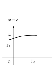
Figure 5: Bifurcating positive solutions of $(R_{\alpha})$ at $(0,c_{a})$.

Proof.

1. First of all, let us observe that once we get positive solutions bifurcating from $\Gamma_{1}$ at $(0,c_{a})$ in $\mathbb{R}\times W^{2,r}(\Omega)$, these ones are in $\mathcal{P}^{\circ}$, since $W^{2,r}(\Omega)\subset C^{1}(\overline{\Omega})$ and $c_{a}$ is a positive constant.

   We use the implicit function theorem to analyze the reduced bifurcation equation $\mathcal{G}(\alpha,t)=0$ around $(0,c_{a})$. Note from (1.3) that $\mathcal{G}(0,c_{a})=0$. Differentiating $\mathcal{G}$ with respect to $t$ yields

   $$\frac{\partial\mathcal{G}}{\partial t}(\alpha,t)=\int_{\Omega}a(x)q(t+\psi)^{q-1}\left(1+\frac{\partial\psi}{\partial t}\right)+\int_{\partial\Omega}\left(1+\frac{\partial\psi}{\partial t}\right).$$

   From (3.8), we see that $\frac{\partial\psi}{\partial t}(0,c_{a})=0$, so that $\frac{\partial\mathcal{G}}{\partial t}(0,c_{a})=\int_{\Omega}a(x)qc_{a}^{\;q-1}+|\partial\Omega|$. Using (1.3), it follows that $\frac{\partial\mathcal{G}}{\partial t}(0,c_{a})=(1-q)|\partial\Omega|>0$. The implicit function theorem is now applicable, and then, we obtain that for $(\alpha,t)\simeq(0,c_{a})$,

   $$\mathcal{G}(\alpha,t)=0\ \Longleftrightarrow\ t=t(\alpha)\ \mbox{with}\ \ t(0)=c_{a}.$$ (3.13)

   Finally, the assertion that $\alpha\mapsto w(\alpha)=t(\alpha)+\psi(\alpha,t(\alpha))$ is $C^{\infty}$ follows from the well known regularity argument for the implicit function theorem.

   The uniqueness assertion can be verified in a similar way as in the proof of Proposition 2.7(ii).

2. Since $w_{n}$ solves $(R_{\alpha_{n}})$ with $\alpha_{n}>0$, we know by Proposition 3.2 that $\{w_{n}\}$ is bounded in $C^{1}(\overline{\Omega})$, and consequently in $H^{1}(\Omega)$. Thus, up to a subsequence, we have $w_{n}\rightharpoonup w$ in $H^{1}(\Omega)$ and $w_{n}\rightarrow w$ in $L^{t}(\Omega)$ for $1\leq t<2^{\ast}$, and in $L^{2}(\partial\Omega)$. Taking the limit as $n\rightarrow\infty$ in the weak formulation of $(R_{\alpha_{n}})$ we see that $w_{n}\rightarrow w$ in $C(\overline{\Omega})$ and $w$ is a nonnegative constant. Moreover, from $\int_{\Omega}a(x)w_{n}^{q}+\int_{\partial\Omega}w_{n}=0$ we obtain $w^{q}\left(\int_{\Omega}a+w^{1-q}|\partial\Omega|\right)=0$, so either $w=0$ or $w=c_{a}$. ∎

Remark 3.12.

Proposition 3.11(i) can be formulated in a more general setting as follows: Assume $(A.0)$, $q_{0}\in[0,1)$, and let $c_{a,q_{0}}$ be $c_{a}$ with $q=q_{0}$. Then $(R_{\alpha})$ has, around $(\alpha,q,w)=(0,q_{0},c_{a,q_{0}})$, exactly one solution $w=w(\alpha,q)\in\mathcal{P}^{\circ}$ parametrized by $(\alpha,q)$, and such that $(\alpha,q)\mapsto w(\alpha,q)=t(\alpha,q)+\psi(\alpha,q,t(\alpha,q))$ is $C^{\infty}$ from $(-\alpha_{0},\alpha_{0})\times(q_{0}-\delta_{0},q_{0}+\delta_{0})$ into $W^{2,r}(\Omega)$ for some $\alpha_{0},\delta_{0}>0$, and $t(0,q_{0})=c_{a,q_{0}}$.

As a corollary of Theorem 1.3 and Propositions 3.2, 3.10 and 3.11, we obtain the following exact multiplicity result for $(R_{\alpha})$:

Corollary 3.13 (Exact multiplicity for $(R_{\alpha})$).

Assume $(A.0)$ and $0<\delta<c_{a}$. Then there exists $\alpha_{\delta}>0$ such that, for each $0<\alpha<\alpha_{\delta}$:

1. $(R_{\alpha})$ has a unique solution $w$ satisfying $\|w\|_{C^{1}(\overline{\Omega})}>\delta$. Moreover, $w=w(\alpha)\in\mathcal{P}^{\circ}$ from Proposition 3.11(i).

2. If we assume, in addition, $(A.1)$ and $q\in\mathcal{A}_{N}$, then $(R_{\alpha})$ has a unique nontrivial solution $w$ satisfying $\|w\|_{C^{1}(\overline{\Omega})}<\delta$, namely, $w=\alpha^{\frac{1}{1-q}}u_{\alpha}\in\mathcal{P}^{\circ}$, where $u_{\alpha}$ is given by Theorem 1.3.

Proof. The first item follows promptly from Propositions 3.2 and 3.11. We prove now the second item. By Theorem 1.3 we know that $\alpha^{\frac{1}{1-q}}u_{\alpha}$ solves $(R_{\alpha})$. We claim that it is the only solution of $(R_{\alpha})$ converging to $0$ in $C^{1}(\overline{\Omega})$ as $\alpha\rightarrow 0^{+}$. Indeed, by Proposition 3.10, if $w_{n}$ is such a solution then $\{u_{n}:=\alpha_{n}^{-\frac{1}{1-q}}w_{n}\}$ remains bounded in $C^{1}(\overline{\Omega})$. Hence, $u_{n}\rightarrow u_{N}$ in $C^{1}(\overline{\Omega})$ by elliptic regularity, Lemma 3.1, and the condition $q\in\mathcal{A}_{N}$. By Theorem 1.3(ii) we infer that for $n$ large enough $u_{n}=u_{\alpha}$ for some $\alpha>0$. The proof is now complete. ∎

We end this section with the corresponding exact multiplicity result for $(P_{\alpha})$, which follows from Corollary 3.13:

Theorem 3.14 (Exact multiplicity for $(P_{\alpha})$).

Assume $(A.0)$, $(A.1)$, and $q\in\mathcal{A}_{N}$. Then there exists $\alpha_{0}>0$ such that $(P_{\alpha})$ has exactly two nontrivial solutions $u_{1,\alpha},u_{2,\alpha}$ for $0<\alpha<\alpha_{0}$. Moreover, $u_{1,\alpha},u_{2,\alpha}\in\mathcal{P}^{\circ}$ and $u_{1,\alpha}<u_{2,\alpha}$ on $\overline{\Omega}$.

4 A topological bifurcation approach to $(R_{\alpha})$

The proof of Theorem 4.4 is based on a bifurcation approach via a regularization scheme, which analyzes the structure of the solutions set of $(R_{\alpha})$. More precisely, we study how the bifurcation curve obtained by Proposition 3.11 behaves globally in $\alpha>0$.

Introducing a new parameter $\varepsilon\in(0,1]$, we consider

$$\begin{cases}-\Delta w=\alpha a(x)(w+\varepsilon)^{q-1}w\ =\alpha a(x)\left(\frac{w}{w+\varepsilon}\right)^{1-q}w^{q}&\mbox{ in }\Omega,\\ w\geq 0&\mbox{ in }\Omega,\\ \partial_{\nu}w=\alpha w&\mbox{ on }\partial\Omega.\end{cases}$$

Note that any nontrivial solution of $(R_{\alpha}^{\varepsilon})$ belongs to $\mathcal{P}^{\circ}$, since $s\mapsto(s+\varepsilon)^{q-1}s$ is $C^{1}$ in $[0,\infty)$, and consequently the strong maximum principle and Hopf’s lemma apply.

We start with some preliminary results, namely, the counterparts of Propositions 3.2, 3.6 and 3.11(ii) for $(R_{\alpha}^{\varepsilon})$.

We establish an a priori estimate in $C^{1}(\overline{\Omega})$ for solutions in $\mathcal{P}^{\circ}$ of $(R_{\alpha}^{\varepsilon})$, i.e. the counterpart of Proposition 3.2:

Proposition 4.1.

Let $\overline{\alpha},\overline{\varepsilon}>0$. Then there exists $\overline{C}>0$ such that $\|w\|_{C^{1}(\overline{\Omega})}\leq\overline{C}$ for every solution $w\in\mathcal{P}^{\circ}$ of $(R_{\alpha}^{\varepsilon})$ with $\alpha\in(0,\overline{\alpha}]$ and $\varepsilon\in(0,\overline{\varepsilon}]$.

Proof. Assume by contradiction that $w_{n}\in\mathcal{P}^{\circ}$ is a solution of $(R_{\alpha_{n}}^{\varepsilon_{n}})$ such that $0<\alpha_{n}\rightarrow\alpha_{\infty}\in[0,\overline{\alpha}]$, $\varepsilon_{n}\in(0,\overline{\varepsilon}]$ but $\|w_{n}\|_{C^{1}(\overline{\Omega})}\rightarrow\infty$. We can then argue as in the proof of Propositions 3.2, with $w_{n}^{q}$ replaced by $\left(\frac{w_{n}}{w_{n}+\varepsilon_{n}}\right)^{1-q}w_{n}^{q}$, and notice that $\left|\frac{w_{n}}{w_{n}+\varepsilon_{n}}\right|\leq 1$ for $n\geq 1$. ∎

The next proposition is the counterpart of Proposition 3.11(ii).

Proposition 4.2.

Assume $(A.0)$ and $\varepsilon\in(0,c_{a})$. If $w_{n}\in\mathcal{P}^{\circ}$ are solutions of $(R_{\alpha_{n}}^{\varepsilon})$ with $\alpha_{n}\rightarrow 0^{+}$ then, up to a subsequence, we have either $w_{n}\rightarrow 0$ or $w_{n}\rightarrow c_{a}-\varepsilon$ in $C(\overline{\Omega})$.

Proof. We use Proposition 4.1 and argue as in the proof of Proposition 3.11(ii) to deduce that, up to a subsequence, $w_{n}\rightarrow c$ in $C(\overline{\Omega})$, where $c$ is a nonnegative constant such that $0=\left(c+\varepsilon\right)^{q-1}c\int_{\Omega}a+c|\partial\Omega|$. The desired conclusion thus follows. ∎

Next we establish an a prori upper bound of $\alpha>0$ for the existence of a solution in $\mathcal{P}^{\circ}$ of $(R_{\alpha}^{\varepsilon})$. Using (1.1), we reduce $(R_{\alpha}^{\varepsilon})$ to the problem

$$\begin{cases}-\Delta u=a(x)\left(\frac{\alpha^{\frac{1}{1-q}}u}{\alpha^{\frac{1}{1-q}}u+\varepsilon}\right)^{1-q}u^{q}&\mbox{ in }\Omega,\\ u\geq 0&\mbox{ in }\Omega,\\ \partial_{\nu}u=\alpha u&\mbox{ on }\partial\Omega.\end{cases}$$

We remark that, as long as $\alpha>0$, $w$ solves $(R_{\alpha}^{\varepsilon})$ if and only if $u=\alpha^{-\frac{1}{1-q}}w$ solves $(P_{\alpha}^{\varepsilon})$. So, it suffices to establish the upper bound for $(P_{\alpha}^{\varepsilon})$.

The following result is the counterpart of Proposition 3.6.

Proposition 4.3.

Assume $(A.3)$. Then, for any $q\in[0,1)$ there exist $\underline{\alpha},\overline{\varepsilon}>0$ such that $(R_{\alpha}^{\varepsilon})$ or $(P_{\alpha}^{\varepsilon})$ has no solutions in $\mathcal{P}^{\circ}$ for any $\alpha>\underline{\alpha}$ and $0<\varepsilon\leq\overline{\varepsilon}$.

Proof. It suffices to consider the case $(P_{\alpha}^{\varepsilon})$, taking (1.1) into account. Let $u\in\mathcal{P}^{\circ}$ be a solution of $(P_{\alpha}^{\varepsilon})$ with $\alpha>0$ and $\varepsilon>0$. Then, Green’s formula yields

$$\int_{\Omega}a(x)\left(\frac{\alpha^{\frac{1}{1-q}}u}{\alpha^{\frac{1}{1-q}}u+\varepsilon}\right)^{1-q}=\int_{\Omega}\frac{-\Delta u}{u^{q}}<-\alpha\int_{\partial\Omega}u^{1-q}.$$

It follows that

$$\alpha\int_{\partial\Omega}u^{1-q}<\int_{\Omega}a^{-}.$$ (4.1)

The rest of the proof proceeds in a similar manner as in the proof of Proposition 3.6. Indeed, let $\beta,\varepsilon_{0}>0$. In place of $(Q_{q,a})$, we consider the following concave mixed problem:

$$\begin{cases}-\Delta u=a(x)f_{\beta,\varepsilon_{0}}(u)&\mbox{in $D$},\\ \partial_{\nu}u=0&\mbox{on $\Gamma_{\partial\Omega}$},\\ u=0&\mbox{on $\Gamma_{\Omega}$},\end{cases}$$ (4.2)

where

$$f_{\beta,\varepsilon}(s):=\left(\frac{\beta^{\frac{1}{1-q}}s}{\beta^{\frac{1}{1-q}}s+\varepsilon}\right)^{1-q}s^{q},\quad s\geq 0.$$

Note that $s\mapsto f_{\beta,\varepsilon}(s)/s$ is decreasing for $s>0$. Since $f_{\beta,\varepsilon}(s)$ is increasing with respect to $\beta>0$ and decreasing with respect to $\varepsilon>0$ for every $s>0$, $u$ is a supersolution of (4.2) for $\alpha\geq\beta$ and $0<\varepsilon\leq\varepsilon_{0}$. Consequently, given $\beta>0$, we can choose $\varepsilon_{0}>0$ small enough such that, denoting by $u_{\beta,\varepsilon_{0}}$ the unique (by Lemma 3.5) positive solution of (4.2) satisfying $u_{\beta,\varepsilon_{0}}>0$ in $D\cup\Gamma_{\partial\Omega}$ (which exists, as in Proposition 3.6), we have that

$$u\geq u_{\beta,\varepsilon_{0}}\quad\mbox{on $\overline{D}$}$$ (4.3)

for $\alpha\geq\beta$ and $0<\varepsilon\leq\varepsilon_{0}$. Combining (4.1) with (4.3) provides the desired conclusion. ∎

Next, under $(A.0)$, we will prove the existence of positive solutions of $(R_{\alpha}^{\varepsilon})$ bifurcating from $\Gamma_{0}$. To obtain bifurcation points from $\Gamma_{0}$ for positive solutions, we consider the linearized eigenvalue problem at $w=0$:

$$\begin{cases}-\Delta\phi=\alpha a(x)\varepsilon^{q-1}\phi&\mbox{ in }\Omega,\\ \partial_{\nu}\phi=\alpha\phi&\mbox{ on }\partial\Omega.\end{cases}$$ (4.4)

Since $(A.0)$ implies that $\int_{\Omega}a\varepsilon^{q-1}+|\partial\Omega|<0$ and $(a\varepsilon^{q-1})^{+}\not\equiv 0$ if $\varepsilon$ is small enough, (4.4) has exactly two principal eigenvalues, namely, $\alpha=0,\alpha_{1,\varepsilon}$, where $\alpha_{1,\varepsilon}>0$ and both are simple. Moreover, (4.4) possesses positive eigenfunctions $\phi_{0},\phi_{1,\varepsilon}$ associated to $0,\alpha_{1,\varepsilon}$, respectively, where $\phi_{0}$ is a positive constant (see [34, Theorem 2.1]).

Applying to both $(0,0)$ and $(\alpha_{1,\varepsilon},0)$ the local and unilateral global bifurcation theory from simple eigenvalues [11, 28, 23], we obtain two components (i.e., nonempty, maximal closed and connected subsets) $\gamma_{0,\varepsilon}$, $\gamma_{1,\varepsilon}$ in $\mathbb{R}\times C^{1}(\overline{\Omega})$ of solutions of $(R_{\alpha}^{\varepsilon})$, containing $(0,0)$ and $(\alpha_{1,\varepsilon},0)$, respectively. In addition, $\gamma_{0,\varepsilon},\gamma_{1,\varepsilon}$ consist of solutions in $\mathcal{P}^{\circ}$ except $(0,0)$, $(\alpha_{1,\varepsilon},0)$. Moreover, the set of nontrivial solutions of $(R_{\alpha}^{\varepsilon})$ near $(0,0)$, $(\alpha_{1,\varepsilon},0)$ is given exactly by $\gamma_{0,\varepsilon}$, $\gamma_{1,\varepsilon}$, respectively, so $\Gamma_{1}\subset\gamma_{0,\varepsilon}$.

Based on the existence of $\gamma_{0,\varepsilon}$, $\gamma_{1,\varepsilon}$, we state the main result of this section, which extends the local existence and multiplicity result proved in [10, Theorem 5.2, Proposition 7.4, Lemma 7.5] by showing that $(R_{\alpha})$ has a subcontinuum of nontrivial solutions for $\alpha>0$.

Theorem 4.4.

Assume $(A.0)$, $(A.1)$, $(A.2)$, $(A.3)$ and $q\in\mathcal{A}_{N}$. Then $(R_{\alpha})$ possesses a subcontinuum $\gamma_{0}$ in $[0,\infty)\times C^{1}(\overline{\Omega})$ of solutions satisfying (3.1) (see Figure 4). Moreover, the following three assertions hold:

1. $u\in\mathcal{P}^{\circ}$ for $(\alpha,u)\in\gamma_{0}\setminus\{(0,0)\}$.

2. There exists $\overline{\alpha}>0$ such that $(R_{\alpha})$ has exactly two nontrivial solutions $w_{1,\alpha},w_{2,\alpha}$ for $0<\alpha<\overline{\alpha}$, which satisfy $(\alpha,w_{1,\alpha})$, $(\alpha,w_{2,\alpha})\in\gamma_{0}$, and $w_{1,\alpha}<w_{2,\alpha}$ on $\overline{\Omega}$. Furthermore,

   1. $w_{1,\alpha}=\alpha^{\frac{1}{1-q}}u_{\alpha}$, where $u_{\alpha}$ is given by Theorem 1.3(ii).

   2. $w_{2,\alpha}=w(\alpha)$, where $w(\alpha)$ is given by Proposition 3.11.

3. Let $\hat{\gamma}_{0}$ be the component of solutions of $(R_{\alpha})$ in $[0,\infty)\times C^{1}(\overline{\Omega})$ that contains $\gamma_{0}$. Then $\hat{\gamma}_{0}\setminus(\Gamma_{0}\cup\Gamma_{1})$ is bounded in $[0,\infty)\times C^{1}(\overline{\Omega})$ (and in $[0,\infty)\times W^{2,r}(\Omega)$, by elliptic regularity) and composed by solutions in $\mathcal{P}^{\circ}$. In addition,

   $$(\hat{\gamma}_{0}\setminus(\Gamma_{0}\cup\Gamma_{1}))\cap\left\{(\alpha,0):\alpha>0\right\}=\emptyset.$$ (4.5)

Proof. First of all, by Proposition 2.3, every nontrivial solution of $(R_{\alpha})$ lies in $\mathcal{P}^{\circ}$.

To prove the existence of $\gamma_{0}$ we shall employ Whyburn’s topological argument [35, (9.12) Theorem], applied to $\gamma_{0,\varepsilon}$, $\gamma_{1,\varepsilon}$. By Propositions 4.1 and 4.3, we infer that $\gamma_{0,\varepsilon}=\gamma_{1,\varepsilon}(=:\gamma_{\varepsilon})$ if $\varepsilon>0$ is small enough, see Figure 6(i). More precisely, Proposition 4.2 and [3, Proposition 18.1] tell us that

$$\gamma_{\varepsilon,+}:=\overline{\{(\alpha,w)\in\gamma_{\varepsilon}:\alpha>0\}},$$

is a bounded (compact) subcontinuum in $[0,\infty)\times C^{1}(\overline{\Omega})$, satisfying

$$\gamma_{\varepsilon,+}\cap\Gamma_{0}=\{(\alpha_{1,\varepsilon},\,0)\},\quad\gamma_{\varepsilon,+}\cap\Gamma_{1}=\{(0,\,c_{a}-\varepsilon)\},$$ (4.6)

see Figure 6(ii).

   

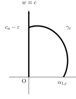
(i)                                            (ii)

Figure 6: The component $\gamma_{\varepsilon}$, and the bounded subcontinuum $\gamma_{\varepsilon,+}$.

Now, let us analyze the limiting behavior of $\gamma_{\varepsilon,+}$ as $\varepsilon\rightarrow 0^{+}$. We introduce the sets

$$\liminf_{\varepsilon\rightarrow 0^{+}}\gamma_{\varepsilon,+}:=\{(\alpha,u)\in\mathbb{R}\times C^{1}(\overline{\Omega}):\lim_{\varepsilon\to 0^{+}}\mathrm{dist}\,((\alpha,u),\gamma_{\varepsilon,+})=0\},$$

$$\limsup_{\varepsilon\rightarrow 0^{+}}\gamma_{\varepsilon,+}:=\{(\alpha,u)\in\mathbb{R}\times C^{1}(\overline{\Omega}):\liminf_{\varepsilon\rightarrow 0^{+}}\mathrm{dist}\,((\alpha,u),\gamma_{\varepsilon,+})=0\}.$$

From the combination of (4.3) and (1.1), it follows that given $\beta>0$, there exists $\varepsilon_{0}>0$ such that $w\geq\beta^{\frac{1}{1-q}}u_{\beta,\varepsilon_{0}}$ on $\overline{D}$ for every solution $w\in\mathcal{P}^{\circ}$ of $(R_{\alpha}^{\varepsilon})$ with $\alpha\geq\beta$ and $0<\varepsilon\leq\varepsilon_{0}$. This implies that $\alpha_{1,\varepsilon}<\beta$ if $0<\varepsilon\leq\varepsilon_{0}$, i.e. $\alpha_{1,\varepsilon}\rightarrow 0$ as $\varepsilon\rightarrow 0^{+}$. In view of (4.6),

$$(0,0),\ (0,c_{a})\in\liminf_{\varepsilon\rightarrow 0^{+}}\gamma_{\varepsilon,+}.$$ (4.7)

In a similar way as in [30, Section 3], we can show that $\bigcup\{\gamma_{\varepsilon,+}:\varepsilon>0\ \mbox{is small}\}$ is precompact. Whyburn’s topological argument [35, (9.12) Theorem] can be now applied to deduce that

$$\gamma_{0,+}:=\limsup_{\varepsilon\rightarrow 0^{+}}\gamma_{\varepsilon,+}$$

is a bounded subcontinuum in $[0,\infty)\times C^{1}(\overline{\Omega})$. In addition, we infer from (4.7) that $(0,0),\ (0,c_{a})\in\liminf_{\varepsilon\rightarrow 0^{+}}\gamma_{\varepsilon,+}\subseteq\gamma_{0,+}$.

Now, we verify that $\gamma_{0,+}$ consists of solutions of $(R_{\alpha})$. Let $(\hat{\alpha},\hat{w})\in\gamma_{0,+}$. By definition, we can choose $\varepsilon_{n}\rightarrow 0^{+}$ and $(\alpha_{n},w_{n})\in\gamma_{\varepsilon_{n}}$ such that $\alpha_{n}\rightarrow\hat{\alpha}\geq 0$ and $w_{n}\rightarrow\hat{w}$ in $C^{1}(\overline{\Omega})$. Since for all $\varphi\in H^{1}(\Omega)$

$$\int_{\Omega}\nabla w_{n}\nabla\varphi=\alpha_{n}\int_{\Omega}a(x)\left(\frac{w_{n}}{w_{n}+\varepsilon_{n}}\right)^{1-q}w_{n}^{q}\varphi+\alpha_{n}\int_{\partial\Omega}w_{n}\varphi,$$

it follows by the Lebesgue dominated convergence theorem that

$$\int_{\Omega}\nabla\hat{w}\nabla\varphi=\hat{\alpha}\int_{\Omega}a(x)\hat{w}^{q}\varphi+\hat{\alpha}\int_{\partial\Omega}\hat{w}\varphi,\quad\forall\varphi\in H^{1}(\Omega).$$ (4.8)

Thus, $\hat{w}$ is a solution of $(R_{\hat{\alpha}})$ by elliptic regularity.

Next, we verify that $\gamma_{0,+}$ is nontrivial, i.e., $\gamma_{0,+}\not\subset\Gamma_{0}\cup\Gamma_{1}$. Since $\gamma_{0,+}$ is connected and joins $(0,0)$ to $(0,c_{a})$, the intermediate value theorem shows that for $0<c<c_{a}$ we can pick $(\hat{\alpha},\hat{w})\in\gamma_{0,+}$ such that $\hat{\alpha}\geq 0$ and $\|\hat{w}\|_{C^{1}(\overline{\Omega})}=c$. We claim that $\hat{\alpha}>0$, i.e. $(\hat{\alpha},\hat{w})\not\in\Gamma_{0}\cup\Gamma_{1}$. To this end, assume by contradiction that $\hat{\alpha}=0$. From the fact that $(\hat{\alpha},\hat{w})\in\gamma_{0,+}$, we infer that there exist $\varepsilon_{n}\to 0^{+}$ and $(\alpha_{n},w_{n})\in\gamma_{\varepsilon_{n},+}$ such that $\alpha_{n}\to 0^{+}$ and $w_{n}\to\hat{w}$ in $C^{1}(\overline{\Omega})$. From (4.8), it follows that $\hat{w}\equiv c$. However, from the definition of $w_{n}$ we obtain that $\int_{\Omega}a(w_{n}+\varepsilon_{n})^{q-1}w_{n}+\int_{\partial\Omega}w_{n}=0$, and so, passing to the limit, that $c=c_{a}$, a contradiction.

Finally, we show how $\gamma_{0,+}$ meets $\Gamma_{0}$ and $\Gamma_{1}$. From Proposition 3.11(ii), we see that $\gamma_{0,+}$ does not meet any point on $\Gamma_{1}$ except $(0,0)$ and $(0,c_{a})$. Moreover, Lemma 3.1 tells us that $\gamma_{0,+}$ does not meet $\Gamma_{0}$, so that $\gamma_{0,+}$ satisfies (3.1).

To sum up, $\gamma_{0}:=\gamma_{0,+}$ is as desired. Indeed, assertion (i) follows from Proposition 2.3. The exactness assertion in (ii) comes from Theorem 3.14. The positivity assertion in (iii) is a consequence of assertion (i), the boundedness assertion follows from Proposition 3.2 and Proposition 3.4, and finally, (4.5) follows from the second assertion of Lemma 3.1. The proof is now complete. ∎

Remark 4.5.

Assuming only $(A.0)$ and $(A.3)$ we can establish, for any $q\in(0,1)$, the existence of a subcontinuum $\gamma_{0}=\{(\alpha,w)\}$ in $[0,\infty)\times C^{1}(\overline{\Omega})$ of solutions of $(R_{\alpha})$ satisfying (3.1) and $w>0$ in $\Omega_{+}^{a}\cup D\cup\Gamma_{\partial\Omega}$ whenever $(\alpha,w)\in\gamma_{0}$. Indeed, if $(\alpha,w)\in\gamma_{0}$ for some $\alpha>0$ then there exist $\varepsilon_{n}\rightarrow 0^{+}$, $\alpha_{n}\rightarrow\alpha$, and $w_{n}\rightarrow w$ in $C^{1}(\overline{\Omega})$ such that $(\alpha_{n},w_{n})\in\gamma_{\varepsilon_{n},+}$, implying that $w_{n}\in\mathcal{P}^{\circ}$ is a solution of $(R_{\alpha_{n}}^{\varepsilon_{n}})$. Applying a sub and supersolutions argument as in the proof of Proposition 4.3 with $u_{n}:=\alpha_{n}^{1/(q-1)}w_{n}$, we deduce that $w>0$ in $\Omega_{+}^{a}\cup D\cup\Gamma_{\partial\Omega}$. Note that Proposition 3.6 still holds for solutions of $(R_{\alpha})$ that are positive in $\Omega_{+}^{a}$, so the component $\hat{\gamma}_{0}=\{(\alpha,w)\}$ of solutions of $(R_{\alpha})$ that includes $\gamma_{0}$ has the same nature as in Theorem 4.4(iii), but is composed now by solutions that are positive in $\Omega_{+}^{a}\cup D\cup\Gamma_{\partial\Omega}$.

Proof of Theorem 1.5.

First we verify (i). The assertion $\alpha_{s}\in\left(0,\infty\right)$ follows from Theorem 1.3(ii) and Propositions 2.3 and 3.4, whereas the second assertion follows from Proposition 3.3, thanks to Theorem 1.2. Assertion (ii) is deduced from Theorem 1.3, Proposition 3.11 and Theorem 3.14. Indeed, $\mathcal{C}_{1}$ is given by Proposition 3.11. Finally, the existence and properties of the component $\mathcal{C}_{\ast}$ in (iii) are proved by combining Theorem 1.3(ii) and Theorem 4.4. ∎