Existence of the tetragonal and rhombohedral deformation families of the gyroid

Abstract.

We provide an existence proof for two 1-parameter families of embedded triply periodic minimal surfaces of genus three, namely the tG family with tetragonal symmetry that contains the gyroid, and the rGL family with rhombohedral symmetry that contains the gyroid and the Lidinoid, both discovered numerically in the 1990s. The existence was previously proved within a neighborhood of the gyroid and the Lidinoid, using Weierstrass data defined on branched rectangular tori. Our main contribution is to extend the technique to branched tori that are not necessarily rectangular.

1. Introduction

A triply periodic minimal surface (TPMS) is a minimal surface $M\subset\mathbb{R}^{3}$ that is invariant under the action of a 3-dimensional lattice $\Lambda$. The quotient surface $M/\Lambda$ then lies in the flat 3-torus $\mathbb{R}^{3}/\Lambda$. The genus of $M/\Lambda$ is at least three, and TPMSs of genus three are abbreviated as TPMSg3s.

Due to their frequent appearance in nature and science, the study of TPMSs enjoys regular contributions from physicists, chemists, and crystallographers. Their discoveries of interesting examples often precede the rigorous mathematical treatment. The most famous example would be the gyroid discovered in 1970 by Alan Schoen [Sch70], then a scientist at NASA. Unlike other TPMSs known at the time, the gyroid does not contain any straight line or planar curvature line, hence it cannot be constructed by the popular conjugate Plateau method [Kar89]. The second TPMSg3 with this property was discovered only twenty years later in 1990, by chemists Lidin and Larsson [LL90], and known nowadays as the Lidinoid. The gyroid and the Lidinoid were later proved to be embedded by mathematicians Große-Brauckmann and Wohlgemuth [GBW96].

By intentionally reducing symmetries of the gyroid and the Lidinoid, two 1-parameter families of TPMSg3s, which we call tG and rGL, were discovered in [FHL93, FH99]; see also [STFH06]. Both families contain the gyroid and retain respectively its rhombohedral and tetragonal symmetries. Remarkably, none of these surfaces contains straight lines or planar curvature lines. Moreover, tG and rGL surfaces are not contained in the 5-parameter family of TPMSg3s constructed by Meeks [Mee90]. Today, the only other explicitly known TPMSg3s outside Meeks’ family are the recently discovered 2-parameter families oH (containing Schwarz’ H) [CW18b] and o$\Delta$ [CW18a].

In [FHL93, FH99], periods were closed only numerically, producing convincing images that leave no doubt for the existence of tG and rGL. Although the importance of numerical discoveries could never be overestimated, the lack of a formal existence proof (that does not involve any numerics) often indicates room for better mathematical understanding. Indeed, our approach in the current paper brings new ways to visualize the tG and rGL surfaces.

An attempt of existence proof for tG and rGL was carried out by Weyhaupt [Wey06, Wey08]. He used the flat structure technique first introduced by Weber and Wolf [WW98, WW02]. Unlike [FHL93, FH99] who parameterized TPMSg3s on branched spheres, Weyhaupt defined Weierstrass data on branched tori. In particular, the gyroid and the Lidinoid, as well as the classical Schwarz’ surfaces, are parameterized on rectangular tori.

Weyhaupt showed that there exists a continuous 1-parameter family of tori that solve the period problems for tG. This family contains the rectangular torus of the gyroid and “does not deform too much from rectangular”. See [Wey08, Lemmas 4.3 & 4.5] for precise statements. Similar results were obtained for an “rG” family near the gyroid and an “rL” family near the Lidinoid. These conclusions, in Weyhaupt’s own word [Wey06, §6.0.6], only asserted “the existence of an analytic family of possibly small parameter space”. In particular, it was not clear that rL and rG are part of the same family, which we call rGL in the current paper. Weyhaupt was aware that, to get away from small neighborhoods, one needs to deal with Weierstrass data defined on non-rectangular tori.

In the current paper, we provide an existence proof for the whole tG and rGL families. More precisely, our main results are

Theorem 1.1 (tG).

There is a 1-parameter family of TPMSg3s containing the gyroid, which we call tG, with the following properties:

• Each TPMSg3 in tG admits a screw symmetry of order 4 around a vertical axis and rotational symmetries of order 2 around horizontal axes.

• tG intersects the tD family and tends to 4-fold saddle towers in the limit.

Theorem 1.2 (rGL).

There is a 1-parameter family of TPMSg3s containing the gyroid and the Lidinoid, which we call rGL, with the following properties:

• Each TPMSg3 in rGL admits a screw symmetry of order 3 around a vertical axis and rotational symmetries of order 2 around horizontal axes.

• rGL intersects the rPD family and tends to 3-fold saddle towers in the limit.

Two properties are listed in each of the statements above. The first specifies the expected symmetries. Weyhaupt [Wey06, Wey08] has proved that TPMSg3s with these symmetries exist in a neighborhood of the gyroid and the Lidinoid. The significance of our work lies in the second property, which states that the 1-parameter family continues in one direction until intersecting Meeks’ family and, in the other direction, to degenerate limits where curvature blows up.

Let us give a preview of our approach.

We will use the same Weierstrass parameterization as Weyhaupt, only more explicit in terms of the Jacobi $\operatorname{sn}$ function. Explicit computations are not possible for non-rectangular tori. However, we notice from the Weierstrass data that the associate family of every tG or rGL surface contains a “twisted catenoid”. These are minimal annuli bounded by curved squares or triangles. Then we generalize a point of view from [GBW96]: As one travels along the associate family, the twisted catenoids open up into gyrating ribbons, and the surface is immersed if adjacent ribbons “fit exactly into each other”. This leads to two expressions for the associate angle, and the period problem asks to find tori for which the two expressions are equal.

It turns out that the torus of an rG or tGL surface is well defined up to a hyperbolic reflection group. The boundary of its fundamental domain corresponds to classical Schwarz’ TPMSg3s, which we understand very well. This already allows us to conclude the existence of the families, all the way to the degenerate limits. We then investigate the asymptotic behavior of the period problem at the limits of the tD or rPD family. This allows us to locate the intersections with Meeks’ family. A uniqueness statement hidden in Weyhaupt’s work [Wey06, Wey08] implies that the families must contain the gyroid, whose embeddedness then ensures the embeddedness of all TPMSg3s in the families.

The paper is organized as follows.

In Section 2, we describe the symmetries of tG and rGL surfaces. This is done by relaxing a rotational symmetry of the classical tP, H and rPD surfaces to a screw symmetry of the same order. We will define a family $\mathcal{T}$ of TPMSg3s with order-4 screw symmetries, which contains the tG family as well as Schwarz’ classical tP, tD and CLP families; we also define a family $\mathcal{R}$ of TPMSg3s with order-3 screw symmetries, which contains the rGL family as well as the classical H and rPD families.

In Section 3, we deduce the Weierstrass data for surfaces in $\mathcal{T}$ and $\mathcal{R}$ from their symmetries. We first prove that surfaces with screw symmetries can be represented as branched covers of flat tori. The symmetries then force the branch points at 2-division points of the tori. This allows us to write down the Weierstrass data explicitly in terms of the Jacobi elliptic function $\operatorname{sn}$. In the end of this section, we establish a convention on the choice of the torus parameter.

In Section 4, we reduce the period problems to just one equation using the twisted catenoids and the ribbon picture. We then give the existence proof in Section 5. The asymptotic analysis is technical hence postponed to the Appendix.

Section 6 is dedicated to discussions. We point out that tG and rGL families provide bifurcation branches that were missing in [KPS14]. We also observe reflection groups that act on $\mathcal{T}$ and $\mathcal{R}$, which provide new ways to visualize the known TPMSg3s. This motivates us to conjecture that the known surfaces are the only surfaces in $\mathcal{T}$ and $\mathcal{R}$. The first step for proving the conjecture is to confirm a uniqueness statement for tG and rGL surfaces.

We assume some familiarity of the reader with classical TPMSg3s including Schwarz’ surfaces, the gyroid, and the Lidinoid. If this is not the case, it is recommended to take a look into [FH92, GBW96, Wey06].

Acknowledgement

The author is grateful to Matthias Weber for constant and helpful conversations. I also thank the anonymous referee, whose useful suggestions to a preliminary version lead to significant improvement of the paper.

2. Symmetries

The tG and rGL families were discovered by relaxing the symmetries of classical surfaces [FHL93, FH99]. It is then a good idea to first recall some classical TPMSg3s, namely the 1-parameter families tP, rPD and H. We recommend the following way to visualize.

tP:

Consider a square catenoid, i.e. a minimal annulus bounded by two horizontal squares related by a vertical translation. Then the order-2 rotations around the edges of the squares generate a tP surface, and any tP surface can be generated in this way.

H:

Consider a triangular catenoid, i.e. a minimal annulus bounded by two horizontal equiangular triangles related by a vertical translation. Then the order-2 rotations around the edges of the triangles generate an H surface, and any H surface can be generated in this way.

rPD:

Similar to the H surfaces, the only difference being that one bounding triangle is reversed.

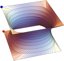
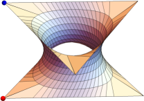
Figure 1. The catenoids that generate tP (left), H (middle) and rPD (right) surfaces.

The catenoids that generate tP, H and rPD surfaces are shown in Figure 1. The 1-parameter families are obtained by vertically “stretching” the catenoids. These families are, remarkably, already known to Schwarz [Sch90]. Reflections might be their most famous and obvious symmetries. But we highlight the following symmetries that will help understanding tG and rGL surfaces.

Inversions:

These are orientation-reversing symmetries shared by every TPMSg3. Meeks [Mee90] proved that every TPMSg3 $M/\Lambda$ has eight inversion centers at the points where Gaussian curvature vanishes. We will come back on that later.

For tP surfaces, the eight inversion centers are at the middle points of the eight bounding edges. For H and rPD surfaces, they are at the middle points of the six bounding edges and the two vertices (up to $\Lambda$) of the bounding triangles.

The catenoids above can be seen as the quotient of $M/\Lambda$ over the inversions. So the fundamental unit $M/\Lambda$ consists of two catenoids. See the top parts of Figures 2 and 3 for how their boundaries identify.

Order-2 rotations around horizontal axes:

These are orientation-preserving symmetries that swap the bounding squares or triangles. So their axes lie in the middle horizontal plane, parallel to the edges and diagonals of the bounding squares or triangles. Up to the inversions, each tP surface has four such rotations, and each H or rPD surface has three.

Rotations around vertical axes:

Up to the inversions, each of these TPMSg3s has exactly one such rotation. The vertical axis passes through the centers of the bounding squares or triangles. This symmetry is orientation-preserving. Its order is 4 for tP and 3 for H and rPD.

Roto-reflections:

A roto-reflection is composed of a rotation around the normal vector at a vertex of the bounding squares or triangles, followed by a reflection in the tangent plane at this vertex. Note that these vertices have vertical normal vectors, hence are poles and zeros of the Gauss map. These symmetries are orientation-reversing. Their order is 4 for tP and 6 for H and rPD.

These symmetries are not independent.

• The rotation around the vertical axis is the composition of two order-2 rotations around horizontal axes.

• Conversely, in the presence of the rotation around the vertical axis, one order-2 rotational symmetry around a horizontal axis implies all the other.

• The roto-reflection arises from the screw symmetry and the inversions.

• For the H and rPD surfaces, [Wey06, Proposition 3.12] asserts that the order-3 rotation around the vertical axis implies the inversion symmetries in the vertices of the triangles.

Hence for TPMSg3s, the symmetries listed above can all be recovered from only two symmetries: the rotational symmetry (of order 3 or 4) around the vertical axis and an order-2 rotational symmetry around a horizontal axis.

It was observed in [GBW96, Lemma 4] that, as one travels along the associate family, all these symmetries are preserved, except for the rotational symmetry around the vertical axis, which is reduced to a screw symmetry. Recall that a screw transform is composed of a rotation and a translation in the rotational axis. The reduction of symmetry can be seen by noticing that the horizontal rotation axes are no longer in the same horizontal plane, hence their compositions induce screw transforms, instead of rotations. Note that the interdependences of the symmetries remain the same after this reduction. In particular, the argument for [Wey06, Proposition 3.12] applies word by word to the order-3 screw symmetry.

The gyroid is in the associate family of Schwarz’ P surface, which is in the intersection of tP and rPD families. Hence the gyroid admits a screw symmetry around a vertical axis and an order-2 rotational symmetry around a horizontal axis. The order of the screw symmetry is 3 or 4, depending on which rotational axes of P is placed vertically. Similarly, the Lidinoid is in the associate family of an H surface, hence admits an order-3 screw symmetry around a vertical axis and an order-2 rotational symmetry around a horizontal axis. As we have discussed, all other symmetries listed above can be recovered from these two.

Remark 2.1.

Interestingly, no other embedded surface is contained in the associate families of the tP, H or rPD surfaces. This follows from a uniqueness statement hidden in the argument of Weyhaupt [Wey06], as we will explain in Section 6.

In the remaining of the paper, for the sake of a uniform treatment of Schwarz’ surfaces and the deformations of the gyroid, we will see rotations as screw transforms with 0 translation. The paper aims at the following two sets of TPMSg3s

• $\mathcal{T}$ consists of embedded TPMSg3s that admit order-4 screw symmetries around vertical axes and order-2 rotational symmetries around horizontal axes.

• $\mathcal{R}$ consists of embedded TPMSg3s that admit order-3 screw symmetries around vertical axes and order-2 rotational symmetries around horizontal axes.

Schwarz’ tP surfaces and the gyroid belong to $\mathcal{T}$. The conjugates of the tP surfaces, namely Schwarz’ tD surfaces, belong to $\mathcal{T}$. We will see that Schwarz’ CLP surfaces also belong to $\mathcal{T}$. Our main Theorem 1.1 states that there exists another 1-parameter family in $\mathcal{T}$, denoted by tG, that contains the gyroid.

Schwarz’ rPD, H surfaces, as well as the gyroid and the Lidinoid belong to $\mathcal{R}$. Our main Theorem 1.2 states that there exists another 1-parameter family in $\mathcal{R}$, denoted by rGL, that contains the gyroid and the Lidinoid.

3. Weierstrass parameterization

We use [Mee90] for general reference about TPMSg3.

Let $M$ be a TPMS invariant under the lattice $\Lambda$. Meeks [Mee90] proved that $M/\Lambda$ is of genus three if and only if it is hyperelliptic, meaning that it can be represented as a two-sheeted branched cover $M/\Lambda\to\mathbb{S}^{2}$ over the sphere. The Gauss map $G$ provides such a branched covering. If $M/\Lambda$ is of genus three, the Riemann-Hurwitz formula implies eight branch points of $G$. We call the corresponding ramification points on $M/\Lambda$ hyperelliptic points. An inversion (in the ambient space $\mathbb{R}^{3}$) in any of the hyperelliptic points induces an isometry that exchanges the two sheets.

Let $z_{1},\dots,z_{8}\in\mathbb{C}$ be the stereographic projections of the Gauss map at the branch points. Now consider the hyperelliptic Riemann surface of genus three defined by

$$w^{2}=P(z)=\Pi_{i=1}^{8}(z-z_{i}).$$

Then we have the following Weierstrass parameterization for $M/\Lambda$:

(1) $$(z,w)\mapsto\operatorname{Re}\int^{(z,w)}\frac{(1-z^{2},(1+z^{2})i,2z)}{w}dz.$$

This parameterization has been widely used for constructing TPMSg3s, ranging from the classical example of Schwarz’ [Sch90] to the tG and rGL families discovered in [FHL93, FH99].

We use the following form of Weierstrass parameterization that traces back to Osserman [Oss64],

(2) $$\Sigma\ni p\mapsto\operatorname{Re}\int^{p}(\omega_{1},\omega_{2},\omega_{3})=\operatorname{Re}\int^{p}\Big{(}\frac{1}{2}\big{(}\frac{1}{G}-G\big{)},\frac{i}{2}\big{(}\frac{1}{G}+G\big{)},1\Big{)}dh\in\mathbb{R}^{3}.$$

Here $\Sigma$ is a Riemann surface, on which $\omega_{1},\omega_{2},\omega_{3}$ must all be holomorphic. In particular, the holomorphic differential $\omega_{3}=dh$ is called the height differential. $G$ denotes (the stereographic projection of) the Gauss map. By comparing (1) and (2), one sees the correspondence $G=z$ and $dh=zdz/w$ (up to a scaling factor $2$). The triple $(\Sigma,G,dh)$ is called Weierstrass data.

The purpose of this section is to determine the Weierstrass data for surfaces in $\mathcal{T}$ and $\mathcal{R}$ from their symmetries. In particular, $\Sigma$ will be a branched torus, whose branch points are determined in Lemmas 3.4 and 3.5. The height differential is determined in Lemma 3.2, and the Gauss map is explicitly given in Lemma 3.7.

3.1. Weierstrass data on tori

Surfaces in $\mathcal{T}$ and $\mathcal{R}$ all admit screw symmetries. The following proposition justifies our choice of branched tori for $\Sigma$.

Proposition 3.1.

If a TPMSg3 $M$ admits a screw symmetry $S$, then $(M/\Lambda)/S$ is of genus one.

Recall that we consider rotational symmetries as special screw symmetries, for which the proposition was proved in [Wey08, Proposition 2.8] but with minor flaws. Hence we include a proof here for completeness.

Proof.

The height differential $dh$ is invariant under $S$, hence descends holomorphically to the quotient $(M/\Lambda)/S$. Since there is no holomorphic differential on the sphere, the genus of $(M/\Lambda)/S$ cannot be $0$.

Recall the Riemann–Hurwitz formula

$$g=n(g^{\prime}-1)+1+B/2.$$

In our case, $g=3$ is the genus of $M/\Lambda$, $g^{\prime}$ is the genus of $(M/\Lambda)/S$, $n$ is the degree of the quotient map, and $B$ is the total branching number. Since the order of a screw symmetry is at least two, we conclude immediately that $g^{\prime}<3$.

It remains to eliminate the case $g^{\prime}=2$. Weyhaupt’s argument in [Wey08] did not accomplish this task. We proceed as follows. Without loss of generality, we may assume the screw axis to be vertical. As Weyhaupt argued, when $g^{\prime}=2$ we have necessarily $n=2$, in which case $G\circ S=-G$. In the parameterization (1), since $dh=zdz/w$ is invariant under $z\mapsto-z$, so must the polynomial $w^{2}=P(z)$, hence we can write $P(z)=Q(z^{2})$, where $Q$ is a polynomial of degree 4. Then $w^{2}=Q(z)$ defines the quotient surface, whose genus is $g^{\prime}=1$. So $g^{\prime}=1$ is the only possibility. ∎

The height differential $dh$, being a holomorphic 1-form on the torus, must be of the form $re^{-i\theta}dz$. Varying the modulus $r$ only results in a scaling. Varying the argument $\theta$ gives the associate family, so we call $\theta$ the associate angle. The following lemma then applies to all TPMSg3s in $\mathcal{T}$ and $\mathcal{R}$.

Lemma 3.2.

If a TPMSg3 $M/\Lambda$ with a screw symmetry $S$ is represented on the branched cover of the torus $(M/\Lambda)/S$, then up to the scaling, the height differential $dh$ must be the lift of $e^{-i\theta}dz$ (note the sign!).

3.2. Locating branch points

By [KK79, Lemma 2(ii)], we know that the order of the screw symmetry $S$ must be $2$, $3$ or $4$. This follows easily from a result of Hurwitz [Hur32], cited in [KK79] as Lemma 1. Moreover, if the order of $S$ is prime, the following formula from [FK92] allows us to calculate the number of fixed points:

$$|\operatorname{fix}(S)|=2+\frac{2g-2g^{\prime}\operatorname{order}(S)}{\operatorname{order}(S)-1}.$$

In particular, a screw symmetry of order 2 fixes exactly four points, and a screw symmetry of order 3 fixes exactly two points. The following lemma follows from the same argument as in [Wey06, Lemmas 3.9, 3.13].

Lemma 3.3.

• If a TPMSg3 $M/\Lambda$ admits a screw symmetry $S$ of order 2, then $G^{2}$ descends to an elliptic function on the torus $(M/\Lambda)/S$ with two simple zeros and two simple poles.

• If $M/\Lambda$ admits a screw symmetry $S$ of order 3, then $G^{3}$ descends to an elliptic function on the torus $(M/\Lambda)/S$ with a double-order zero and a double-order pole.

We now try to locate the branch points of the covering map for surfaces in $\mathcal{T}$ and $\mathcal{R}$. Since the ramification points on $M/\Lambda$ are all poles and zeros of the Gauss map, our main tool is naturally Abel’s Theorem, which states that the difference between the sum of poles and the sum of zeros (counting multiplicity) is a lattice point.

A surface in $\mathcal{T}$ admits a screw symmetry $S$ of order 4, $S^{2}$ is then a screw symmetry of order 2. Recall that $S$ and the inversions induce roto-reflectional symmetries of order 4 centered at the poles and zeros of the Gauss map. They descend to the quotient torus $(M/\Lambda)/S^{2}$ as inversions in the branch points of the covering map.

Lemma 3.4 (Compare [Wey06, Lemma 3.10]).

Let $M$ be a TPMSg3 admitting a screw symmetry $S$ of order 4, hence parameterized on a branched double cover of the torus $(M/\Lambda)/S^{2}$. If one branch point is placed at $0$, then the other branch points must be placed at the three 2-division points of the torus.

Proof.

We may assume that the branch point at $0$ corresponds to a zero of $G^{2}$. If a pole $p$ is not at any 2-division points, $-p$ must be a different pole by the roto-reflection. Then Abel’s Theorem forces the other zero to be at a lattice point, which is absurd. So both poles must be placed at 2-division points. Then Abel’s Theorem forces the other zero at the remaining 2-division point. ∎

Note that the screw symmetry of order 4 descends to the quotient torus as the translation that swaps the zeros.

Lemma 3.5 ([Wey06, Lemma 3.13]).

Let $M$ be a TPMSg3 admitting a screw symmetry $S$ of order 3, hence parameterized on a branched triple cover of the torus $(M/\Lambda)/S$. If one branch point is placed at $0$, then the other branch points must be placed at the three 2-division points of the torus.

Proof.

We may assume that the branch point at $0$ corresponds to a double-order zero of $G^{3}$. Then the Abel’s Theorem forces the double-order pole to be at a 2-division point. ∎

3.3. An explicit expression for the Gauss map

The locations of poles and zeros determine an elliptic function up to a complex constant factor. Elliptic functions with poles and zeros at lattice points and 2-division points are famously given by Jacobi elliptic functions. In particular, $\operatorname{sn}(z;\tau)$ is an elliptic function with periods $4K$ and $2iK^{\prime}$. Its zeros lie at $0$ and $2K$, and poles at $iK^{\prime}$ and $2K+iK^{\prime}$. Here, $K$ is the complete elliptic integral of the first kind with modulus $m=\lambda(2\tau)$, $\lambda$ is the modular lambda function, and $K^{\prime}:=-2i\tau K$.

We use [Law89] as the major reference for elliptic functions. Other useful references include [Bow61, BF71, BB98] and NIST’s Digital Library of Mathematical Functions [DLMF].

Remark 3.6.

Note that we do not define $K^{\prime}(m)=K(1-m)$, and our $\tau$ is half of the traditional definition but coincides with the definition on page 226 of [Law89].

Since $\operatorname{sn}$ has the expected zeros and poles, we may write the Gauss map $G$ for a $\mathcal{T}$ surface as

$$G^{2}=\rho\operatorname{sn}(4Kz;\tau).$$

In particular, the factor $4K$ on the variable $z$ brings the defining torus to $\mathbb{C}/\langle 1,\tau\rangle$, which is more convenient for us. The zeroes of $G^{2}$ are at $0$ and $1/2$, and the poles at $\tau/2$ and $(\tau+1)/2$. The complex factor $\rho$ is known as the López–Ros factor [LR91] in the minimal surface theory. Varying its argument only results in a rotation of the surface in the space, hence only the norm $|\rho|$ concerns us.

The multi-valued function on $\mathbb{C}/\langle 1,\tau\rangle$ is given by $G=[\rho\operatorname{sn}(4Kz;\tau)]^{1/2}$. We take the branch cuts of the square root along the segments $[0,\tau/2]$ and $[(\tau+1)/2,\tau+1/2]$, compatible with [Wey06]; see Figure 2. None of the branch points is hyperelliptic point. Instead, the symmetry $\operatorname{sn}(2K-z)=\operatorname{sn}(z)$ reveals four other inversion centers at $1/4$, $3/4$, $1/4+\tau/2$ and $3/4+\tau/2$, and they lift to eight hyperelliptic points.

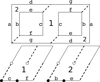
Figure 2. Top: Identifying segments with the same labels yields a surface of genus three. The numbered regions are fundamental domains of the screw symmetry of order 3. Bottom: Branch cuts in the branched torus for $\mathcal{T}$ surfaces. Solid circles are zeros; empty circles are poles.

Similarly, we may write the Gauss map $G$ for an $\mathcal{R}$ surface as

$$G^{3}=[\rho\operatorname{sn}(4Kz;\tau)]^{2}$$

where $\rho$, again, is the López–Ros factor. This function is well defined on the torus $\mathbb{C}/\langle 1/2,\tau\rangle$, halving the defining torus of $\operatorname{sn}(z;\tau)$. $G^{3}$ has a double-order zero at $0$ and a double-order pole at $\tau/2$, as expected. The multi-valued function on $\mathbb{C}/\langle 1/2,\tau\rangle$ is given by $G=[\rho\operatorname{sn}(4Kz;\tau)]^{2/3}$. We take the branch cuts of the cubic root along the segments $[0,\tau/2]$, $[\tau/2,\tau]$, $[1/2,(\tau+1)/2]$ and $[(\tau+1)/2,\tau+1/2]$, compatible with [Wey06]; see Figure 3. This time, both branch points are hyperelliptic points; cf. [Wey06, Proposition 3.12]. We recognize two other inversion centers at $1/4$ and $1/4+\tau/2$, which lift to six more hyperelliptic points.

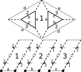
Figure 3. Top: Identifying segments with the same labels yields a surface of genus three. The numbered regions are fundamental domains of the screw symmetry of order 2. Bottom: Branch cuts in the branched torus for $\mathcal{R}$ surfaces. Solid circles are zeros; empty circles are poles.

For surfaces in $\mathcal{T}$ and $\mathcal{R}$, the López–Ros factor $\rho$ can be determined by the order-2 rotational symmetries that swap the poles and zeros of the Gauss map. More specifically, $G^{2}$ and $1/G^{2}$ for $\mathcal{T}$ must have the same residue at their respective poles, and $G^{3}$ and $1/G^{3}$ for $\mathcal{R}$ must have the same principal parts at their poles. By the identity $\operatorname{sn}(z+iK^{\prime};\tau)=1/\sqrt{m}\operatorname{sn}(z;\tau)$, we deduce that $\rho=m^{1/4}$ for both $\mathcal{T}$ and $\mathcal{R}$.

We have shown that

Lemma 3.7.

Up to a rotation in $\mathbb{R}^{3}$, the Gauss map $G$ have the form

$$G =[m^{1/4}\operatorname{sn}(4Kz;\tau)]^{1/2} \mathcal{T}$$ for a surface in , and

$$G =[m^{1/4}\operatorname{sn}(4Kz;\tau)]^{2/3} \mathcal{R}$$ for a surface in .

Remark 3.8.

Equivalently, we can write the Gauss map for $\mathcal{T}$ in the form

$$G^{2}=\rho^{\prime}\frac{\theta(z)\theta(z-1/2)}{\theta(z-\tau/2)\theta(z-1/2+\tau/2)}$$

where $\theta$ is the Jacobi Theta function (actually one of them) for the lattice $\mathbb{C}/\langle 1,\tau\rangle$, and the López–Ros factor $\rho^{\prime}=e^{-i\pi(\tau-1)/2}$. The Gauss map for $\mathcal{R}$ may have a similar expression. This should help the readers to compare our computation with those in [Wey06, Wey08].

Remark 3.9.

With a change of basis for the torus, one could, of course, use other Jacobi elliptic functions to express the Gauss map. We notice that the normalized Jacobi function $m^{1/4}\operatorname{sn}(z;\tau)$ is one of the three Jacobi-type elliptic functions constructed in [KWH93, § 3], where the symmetry is thoroughly investigated.

3.4. Conventions on the torus

Recall that the modular lambda function is invariant under the congruence subgroup $\Gamma(2)$. Hence $m=\lambda(2\tau)$ and $\operatorname{sn}(z;\tau)$ are invariant under the congruence subgroup $\Gamma_{0}(4)$ generated by the transforms $\tau\mapsto\tau+1$ and $\tau\mapsto\tau/(1-4\tau)$. So the Weierstrass data is invariant under $\Gamma_{0}(4)$, and we have infinitely many choices of $\tau$ for each surface in $\mathcal{T}$ or $\mathcal{R}$. In fact, using Jacobi $\operatorname{sn}$ function already limits the choice.

Surfaces in [Wey06, Wey08] all admit reflectional symmetries, making it possible to choose $\tau$ to be pure imaginary, so the torus is rectangular (and a different elliptic function should be used). We could not use this convention since, in general, the tG and rGL surfaces do not admit reflectional symmetry, nor do surfaces in their associated families.

The fundamental domain of $\Gamma(2)$ is usually taken as the region $C$ bounded by the vertical lines $\operatorname{Re}\tau=\pm 1$ and the half circles $|\tau\pm 1/2|=1/2$. It is then natural to choose $2\tau$ in this region, so $\tau$ is in the region $C/2$ bounded by $\operatorname{Re}\tau=\pm 1/2$ and $|\tau\pm 1/4|=1/4$, a fundamental domain of $\Gamma_{0}(4)$. Under this convention, our $K^{\prime}$ coincides with the standard associated elliptic integral of the first kind with modulus $m$; then we can safely employ the formula in most textbooks.

This natural choice is, however, not convenient for analyzing the tG and rGL families. For instance, the tP and tD families correspond to the same vertical line $\operatorname{Re}\tau=0$, and the gyroid also lies on this line. In fact, we will see that, for each $r\in(-1/2,0)\cup(0,1/2]$, there are two members of tG with $\operatorname{Re}\tau=r$ under the natural convention. The same happens for rGL. Hence we need a different convention.

We will see that, for a surface in $\mathcal{T}$ or $\mathcal{R}$, the poles and zeros of the Gauss map are aligned along vertical lines, alternatingly arranged and equally spaced. For the sake of a uniform treatment, we make the following convention:

Convention.

For surfaces in $\mathcal{T}$ and $\mathcal{R}$, we assume that the Weierstrass parameterization maps $(1+\tau)/2$ directly above $0$.

Our convention should be seen as a marking on the surface. Although the Weierstrass data is invariant under the transform $\tau\mapsto\tau+1$, the marked branch point $(1+\tau)/2$ is however different. The marking then serves to distinguish, for instance, Schwarz’ P, D surfaces and the gyroid. We will see that, under our convention, $\operatorname{Re}\tau=0$ corresponds to the gyroid in $\mathcal{T}$ and the Lidinoid in $\mathcal{R}$.

We list in Table 1 the Weierstrass data of classical TPMSg3 under our convention. For each family, we specify the possible $\tau$ for the torus and the associate angle $\theta$. We also accompany a diagram, showing the possible $\tau$ (dashed curve), the fundamental parallelogram for a typical example, the poles (empty circles) and the zeros (solid circles) of $\operatorname{sn}(z;\tau)$ (whose defining torus could twice the shown quotient torus!), and an arrow indicating $dh$ by pointing to the direction of increasing height. The bottom-left corner of the parallelogram is always 0, the bottom edge represents 1 for $\mathcal{T}$ or 1/2 for $\mathcal{R}$, and the left edge always represents $\tau$. The tori used in [Wey06, Wey08] are shown as dotted rectangles for reference.

tP:	$\operatorname{Re}\tau=-1$,	$\theta=\pi/2$,
tD:	$\operatorname{Re}\tau=1$,	$\theta=0$,
CLP:	$|\tau+1/2|=1/2$,	$\theta=\arg\tau-\pi/2$,
H:	$\operatorname{Re}\tau=-1$,	$\theta=\pi/2$,
rPD:	$\operatorname{Re}\tau=1/2$,	$\theta=\pi/2$ or $0$,

Table 1. Weierstrass data for classical TPMSg3.

4. Period conditions

Rectangular tori are convenient in many ways. For example, many straight segments in the branched torus correspond to geodesics on the surface, making it possible to compute explicitly [Wey06]. With general tori, we lose all the nice properties. An explicit computation is indeed hopeless, but we are still able to say something.

4.1. Twisted catenoids

Assume $dh=e^{-i\pi/2}=-idz$ for the moment. We now study the image under the maps

$$\Phi_{i}:\mathbb{C} \to\mathbb{C}\qquad i=1,2$$

$$\Phi_{1}:z \mapsto\int^{z}dh\cdot G$$

$$\Phi_{2}:z \mapsto\int^{z}dh/G.$$

Let us first look at the lower half of the branched torus of $\mathcal{T}$, i.e. the part with $0<\operatorname{Im}z<\operatorname{Im}\tau/2$. This is topologically an annulus and lifts to its universal cover $\{z|0<\operatorname{Im}z<\operatorname{Im}\tau/2\}$, which is a strip in $\mathbb{C}$. By analytic continuation, $G$ lifts to a function of period $2$ on the strip. The boundary lines $\operatorname{Im}z=0^{+}$ and $\operatorname{Im}z=\operatorname{Im}\tau/2-0^{+}$ are then mapped by $\Phi_{1}$ into periodic or closed curves.

By the same argument as in the standard proof of the Schwarz–Christoffel formula (see also [Wey06, FW09]), we see that the curves make an angle at each branch point. The interior angle is $\pi/2$ at the poles of $G^{2}$ and $3\pi/2$ at the zeros. By the symmetry $\operatorname{sn}(2K+z;\tau)=-\operatorname{sn}(z;\tau)$, the image of the segments $[n/2,(n+1)/2]$, $n\in\mathbb{Z}$, are all congruent, and images of adjacent segments only differ by a rotation of $\pi/2$ around their common vertex. Moreover, by the symmetry $\operatorname{sn}(2K-z;\tau)=\operatorname{sn}(z;\tau)$, the image of each segment admits an inversional symmetry. The inversion center is the image of the hyperelliptic points, at the midpoint of each segment. The same can be said about the segments $[(n+\tau)/2,(n+1+\tau)/2]$, $n\in\mathbb{Z}$.

Therefore, the boundaries of the strip are mapped to closed curves with a rotational symmetry of order $4$. The curves look like “curved squares”, obtained by replacing the straight edges of the square by congruent copies of a symmetric curve. Moreover, the two twisted squares share the same rotation center. The strip is then mapped by $\Phi_{1}$ to the twisted annulus bounded by the curved squares. See Figure 4.

A similar analysis can be carried out on the upper annulus $\operatorname{Im}\tau/2<\operatorname{Im}z<\operatorname{Im}\tau$. However, the branch cuts ensure that the two annuli continuous into different branches (different signs of square root) when crossing the segments $[n/2,n/2+\tau]$. As a consequence, the boundary curves is turning in the opposite direction. As one passes through the segment $[\tau/2,(\tau+1)/2]$, the images of $\Phi_{1}$ is extended by an inversion, which reverses orientation.

Because of our choice of the López–Ros parameter, the image of the lower annulus under $\Phi_{2}$ is congruent to the image of the upper annulus under $\Phi_{1}$. The only difference is that the inner and the outer boundaries of the annulus are swapped. See Figure 4.

Figure 4. Plot of the lower annulus $0<\operatorname{Im}z<\operatorname{Im}\tau/2$ under the maps $\Phi_{1}$ and $\Phi_{2}$ for $\mathcal{T}$, with $\tau=0.3+0.2i$.

Combining the flat structures $\Phi_{1}$ and $\Phi_{2}$ gives us the image under the Weierstrass parameterization. Because of our choice of $dh$, we know that the lines $\operatorname{Im}z=0$ and $\operatorname{Im}z=\operatorname{Im}\tau/2$ are mapped to two horizontal planar curves, at heights $0$ and $\operatorname{Im}\tau/2$ respectively. The previous analysis tells us that these are two congruent closed curves that look like curved squares. In particular, they admit rotational symmetry of order $4$. The strip $0<\operatorname{Im}z<\operatorname{Im}\tau/2$ is then mapped to a “twisted square catenoid” bounded by these curves. Moreover, the twisted catenoid admits rotational symmetries of order 2 around horizontal axes that swap its boundaries. See Figure 5.

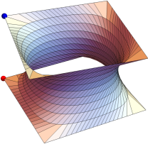
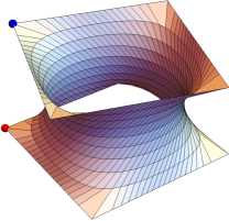
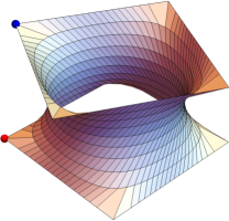
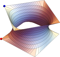
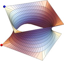
Figure 5. Plot of the annulus with $0<\operatorname{Im}z<\operatorname{Im}\tau/2$ under the Weierstrass parameterization of $\mathcal{T}$, for $\operatorname{Im}\tau=1$ and $\operatorname{Re}\tau=-1,-0.9,-0.8,-0.7,-0.6,-0.5$, in this order. The red and the blue points indicate the images of $0$ and $(1+\tau)/2$. An increasing “twist angle” is visible. Note that bounding edges are in fact slightly curved, except for $\operatorname{Re}\tau=-1$ and $-0.5$.

Inversion in the midpoint of a curved edge extends the surface with another twisted square catenoid, which is the image of the strip $\operatorname{Im}\tau/2<\operatorname{Im}z<\operatorname{Im}\tau$. Repeated inversions in the midpoints of the curved edges extend the catenoid infinitely into the space $\mathbb{R}^{3}$, but the result is usually not embedded.

The same argument applies to the Weierstrass data of $\mathcal{R}$. The lower annulus lift to a strip in $\mathbb{C}$ of period $3/2$. We then obtain a twisted triangular catenoid with rotational symmetry of order $3$, and repeated inversions in the midpoints of the curved edges extend the catenoid infinitely into $\mathbb{R}^{3}$, but usually not embedded. See Figures 6 and 7.

Figure 6. Plot of the annulus $0<\operatorname{Im}z<\operatorname{Im}\tau/2$ under the maps $\Phi_{1}$ and $\Phi_{2}$ for $\mathcal{R}$, with $\tau=0.3+0.2i$.

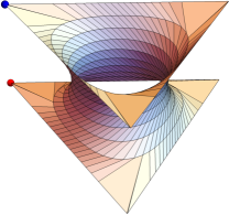
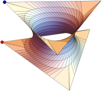
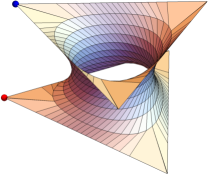
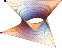
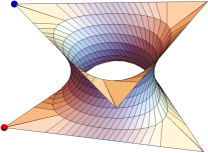
Figure 7. Plot of the annulus with $0<\operatorname{Im}z<\operatorname{Im}\tau/2$ under the Weierstrass parameterization of $\mathcal{R}$, for $\operatorname{Im}\tau=1$ and $\operatorname{Re}\tau=-1,-0.9,-0.8,-0.7,-0.6,-0.5$, in this order. The red and the blue points indicate the images of $0$ and $(1+\tau)/2$. An increasing “twist angle” is then visible. Note that bounding edges are in fact slightly curved, except for $\operatorname{Re}\tau=-1$ and $-0.5$.

It is interesting to observe the twisted catenoids when $\operatorname{Re}\tau$ increases.

Let us start from a tP surface with $\operatorname{Re}\tau=-1$. Its catenoid is the standard square catenoid, not twisted. As we increase $\operatorname{Re}\tau$, the square catenoid becomes “twisted” in two senses: on the one hand, the bounding squares become curved; on the other hand, horizontal projections of the squares form an angle. This “twist angle” seems to increase monotonically with $\operatorname{Re}\tau$ (we are not sure!); see Figure 5. Remarkably, when $\operatorname{Re}\tau=-1/2$, reflectional symmetry is restored in the Weierstrass data, and the catenoid is bounded by two straight squares forming a twist angle of $\pi/4$.

Then the catenoid is again “twisted” as we continue to increase $\operatorname{Re}\tau$ until $1$. During the process, the twist angle increases from $0$ at $\operatorname{Re}\tau=-1$ (tP), to $\pi/4$ at $\operatorname{Re}\tau=-1/2$, to $\pi/2$ at $\operatorname{Re}\tau=0$ (gyroid), to $3\pi/4$ at $\operatorname{Re}\tau=1/2$, until $\pi$ at $\operatorname{Re}\tau=1$ (tD). These are the only cases where reflectional symmetry is restored, and the bounding edges are straight. The term “twist angle” is in general ill-defined, but carries a natural meaning in these cases. Note that, although the transform $\tau\mapsto\tau+1$ leaves the catenoid invariant, the image of $(\tau+1)/2$ (blue point in Figure 5) is however rotated by $\pi/2$. So the marked twisted catenoid is invariant under the transform $\tau\mapsto\tau+4$.

Remark 4.1.

The tG surfaces at $\operatorname{Re}\tau=\pm 1/2$ deserve more attention, as the reflectional symmetries in their Gauss maps seem special.

Similarly, for $\mathcal{R}$, we can start from the triangular catenoid of H with $\operatorname{Re}\tau=-1$, and increase $\operatorname{Re}\tau$ until $1/2$. The bounding triangles become curved and form a twisted angle that seems to increase monotonically with $\operatorname{Re}\tau$; see Figure 7. In particular, the “twist angle” increases from $0$ at $\operatorname{Re}\tau=-1$ (H), to $\pi/3$ at $\operatorname{Re}\tau=-1/2$ (gyroid), to $2\pi/3$ at $\operatorname{Re}\tau=0$ (Lidinoid), until $\pi$ at $\operatorname{Re}\tau=1/2$ (rPD). These are the only cases where the reflectional symmetry is restored, the bounding edges are straight, and the meaning of the “twist angle” is clear. The marked twisted catenoid is invariant under the transform $\tau\mapsto\tau+3$.

4.2. Vertical and horizontal associate angles

The Weierstrass parameterization defines an immersion only if the period problems are solved. That is, the integrations around closed curves on $\Sigma$ should all vanish (up to $\Lambda$). The period problems for Schwarz’ surfaces were explicitly solved in [Wey06].

Große–Brauckmann and Wohlgemuth [GBW96] proposed a convenient way to visualize the gyroid, which we now generalize to all surfaces in $\mathcal{T}$ and $\mathcal{R}$. This will reduce the period problems to just one equation.

We have demonstrated a twisted catenoid in the associate family of every surface in $\mathcal{T}$ or $\mathcal{R}$. As one travels from the twisted catenoids along the associate family, the bounding twisted squares or triangles become “twisted helices”, and the twisted catenoid opens up into a ribbon bounded by these helices.

For an embedded TPMSg3 $M/\Lambda$, Meeks [Mee90] proved that its hyperelliptic points can be identified to the lattice and half-lattice points of $\Lambda$. Then the symmetries of $\mathcal{T}$ and $\mathcal{R}$ imply that the poles and zeros of the Gauss map are

• aligned along vertical lines arranged in a square or triangular lattice and

• alternatingly arranged and equally spaced on each vertical line.

Conversely, if these are the cases, then the two ribbons forming the fundamental unit “fit exactly into each other”. That is, their boundaries are identified in the same pattern as the twisted catenoids (see Figures 2 and 3). This is guaranteed by the screw and the inversional symmetries. So the properties listed above form a sufficient condition for the immersion.

To be more precise, we define the pitch of a helix to be the increase of height after the helix makes a full turn. Then the poles and zeros are alternatingly arranged and equally spaced on each vertical line if the pitch of each helix is an even multiple of the minimum vertical distance between the poles and the zeros. In particular, for the gyroid, the pitch doubles the minimum vertical distance. So we expect the same property for tG and rGL surfaces.

Remark 4.2.

The ratio of the pitch over the minimum vertical distance can also take other values. They will be discussed in Section 6.

For tG surfaces, this means that the integral of the height differential $dh$ from $0$ to $2$ doubles the integral from $0$ to $(1+\tau)/2$. Or equivalently, the integral from $0$ to $1$ equals the integral from $0$ to $(1+\tau)/2$. This can be easily achieved by adjusting the associate angle $\theta$ to (compare [Wey08, Definition 4.2])

$$\theta=\theta_{v}(\tau)=\arg(\tau-1)-\pi/2\quad\text{for tG.}$$

Similarly, for rGL surfaces, this means that the integral of $dh$ from $0$ to $3/4$ equals the integral from $0$ to $(1+\tau)/2$. Then we deduce that

$$\theta=\theta_{v}(\tau)=\arg(\tau-1/2)-\pi/2\quad\text{for rGL.}$$

We now calculate the associate angle in another way, using the fact that the images of $0$ and $(1+\tau)/2$ are vertically aligned, i.e. have the same horizontal coordinates.

First note that, by the symmetry $\operatorname{sn}(2K+iK^{\prime}-z;\tau)=1/\operatorname{sn}(z;\tau)$, we have the identity

$$\int_{0}^{(1+\tau)/2}dz/G=\int_{0}^{(1+\tau)/2}dz\cdot G=:\psi(\tau)$$

We may place the image of $0$ at the origin. First look at the surface with $\theta=0$, hence $dh=dz$. Then the horizontal coordinates of the image of $(1+\tau)/2$ are

$$\operatorname{Re}\int_{0}^{(1+\tau)/2}\Big{(}\frac{1}{2}\big{(}\frac{1}{G}-G\big{)},\frac{i}{2}\big{(}\frac{1}{G}+G\big{)}\Big{)}dz=(0,-\operatorname{Im}\psi(\tau)).$$

Then we look at the surface with $\theta=\pi/2$, hence $dh=e^{-i\pi/2}dz=-idz$ (the conjugate surface). Then the coordinates are

$$\operatorname{Re}\int_{0}^{(1+\tau)/2}\Big{(}-\frac{i}{2}\big{(}\frac{1}{G}-G\big{)},\frac{1}{2}\big{(}\frac{1}{G}+G\big{)}\Big{)}dz=(0,\operatorname{Re}\psi(\tau)).$$

So for the surface with associate angle $\theta$, the first coordinate is always $0$, while the second coordinate

$$-\cos\theta\operatorname{Im}\psi(\tau)+\sin\theta\operatorname{Re}\psi(\tau)$$

vanishes when

$$\theta=\theta_{h}(\tau):=\arg\psi(\tau).$$

We have shown that

Lemma 4.3.

The Weierstrass data given by Lemmas 3.2 and 3.7 define an immersion if and only if

$$\theta_{h}(\tau)=\theta_{v}(\tau),$$

or more explicitly,

(3) $$\arg\psi(\tau)=\begin{cases}\arg(\tau-1)-\pi/2&\text{for $\mathcal{T}$;}\\ \arg(\tau-1/2)-\pi/2&\text{for $\mathcal{R}$.}\end{cases}$$

We are finally ready to give the existence proof.

5. Existence proof

5.1. tG family

In Figure 8, we show for $\mathcal{T}$ the numerical solutions to (3) with $-1<\operatorname{Re}\tau<1$, accompanied by two half-circles representing the CLP family. Our task is to prove the existence of the continuous 1-parameter solution curve that we see in the picture, which we call the tG family. Let the shaded domain in the figure be denoted by

$$\Omega_{t}:=\{\tau\mid\operatorname{Im}\tau>0,-1<\operatorname{Re}\tau<1,|\tau\pm 1/2|>1/2\}.$$

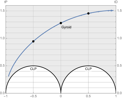
Figure 8. Solutions for $\mathcal{T}$ to (3) with $-1<\operatorname{Re}\tau<1$.

Proposition 5.1.

There exists a continuous 1-dimensional curve of $\tau$ in $\Omega_{t}$ that solves (3). This curve tends to $-1$ at one end and to $1+ti$ for some $0<t<\infty$ at the other end. Moreover, the TPMSg3s represented by points on the curve are all embedded.

Proof.

We examine the angles $\theta_{v}$ and $\theta_{h}$ on the boundaries of $\Omega_{t}$.

On the vertical line $\operatorname{Re}\tau=-1$, we see immediately that $0<\theta_{v}<\pi/2$. Since this line corresponds to the tP family, we know very well that the image of $(1+\tau)/2$ is directly above the image of $0$ when $dh=e^{-i\pi/2}dz$. Hence $\theta_{h}=\pi/2>\theta_{v}$.

The half-circle $|\tau+1/2|=1/2$ corresponds to the CLP family. We know very well that the image of $(1+\tau)/2$ is directly above the image of $0$ when $dh=\exp(-i(\arg\tau-\pi/2))dz$, so $\theta_{h}=\arg\tau-\pi/2$. Then the inequality $\theta_{h}<\theta_{v}$ follows from elementary geometry.

On the half-circle $|\tau-1/2|=1/2$, it follows from elementary geometry that $\theta_{v}=\arg\tau$. This half-circle corresponds again to the CLP family. When $dh=\exp(-i\theta_{v})dz$, the image of $\tau/2$ is directly above the image of $0$. In this case, we know very well that the flat structure of $\Phi_{1}$ is as depicted in Figure 9; see [Wey06]. In particular, we have

$$\arg\int_{0}^{(1+\tau)/2}dh\cdot G=\arg\int_{0}^{(1+\tau)/2}dz\cdot G\exp(-i\theta_{v})=\theta_{h}-\theta_{v}<0,$$

hence $\theta_{h}<\theta_{v}$.

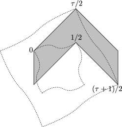
Figure 9. Image of the rectangle with vertices at $0$, $1/2-\tau/2$, $1/2+\tau/2$, $\tau$, under the map $\Phi_{1}$ for a CLP surface (the grey area). The twisted square annulus is sketched (exaggeratedly) in dashed curves.

On the vertical line $\operatorname{Re}\tau=1$, we see immediately that $\theta_{v}=0$. Since this line corresponds to the tD family, we know very well that the image of $(1+\tau)/2$ is directly above the image of $0$ when $dh=dz$, so $\theta_{h}=0$. Hence this line solves the period condition $\theta_{h}=\theta_{v}$, but not very helpful for our proof.

As $\operatorname{Im}\tau\to\infty$, we see immediately that $\theta_{v}\to 0$. Asymptotic behavior of $\theta_{h}$ is technical, so we postpone the details to Appendix, where Lemma A.2 states that $\theta_{h}\to\operatorname{Re}(1-\tau)\pi/4$. Hence $\theta_{h}>\theta_{v}$ for $\operatorname{Im}\tau$ sufficiently large.

Now consider $\tau=1-\epsilon+i\eta$ for small $\epsilon$. It is immediate that the derivative of $\theta_{v}$ with respect to $\epsilon$ at $\epsilon=0$ is $1/\eta$, hence tends to $0$ as $\eta\to\infty$. Meanwhile, the asymptotic behavior of $\theta_{h}$ tells us that $\partial\theta_{h}/\partial\epsilon\to\pi/4>0$ as $\eta\to\infty$. Consequently, there exist two positive numbers $H$ and $\delta$ such that $\theta_{h}(1-\epsilon+\eta i)>\theta_{v}(1-\epsilon+\eta i)$ for all $\eta>H$ and $\epsilon<\delta$.

As $\tau\to 1$ within $\Omega_{t}$, Lemma A.3 in Appendix claims that $\theta_{h}(\tau)\to 0$ from the negative side, but one sees immediately that $\theta_{v}(\tau)\to 0$ from the positive side. Consequently, there exists a neighborhood $U$ of $1$ such that $\theta_{h}(\tau)<\theta_{v}(\tau)$ for all $\tau\in U\cap\Omega_{t}$.

Note that $\theta_{h}$ and $\theta_{v}$ are both real analytic functions in the real and imaginary part of $\tau$, hence the solution set of the period condition (3) is an analytic set. By the continuity, we conclude that the solution set contains a connected component that separates the half-circles $|\tau\pm 1/2|=1/2$ from the line $\operatorname{Re}\tau=-1$ and the infinity. Moreover, this set must also separate a neighborhood $U$ of $1$ from the set $\{\tau\mid\operatorname{Re}\tau>1-\delta,\operatorname{Im}\tau>H\}$. Because of the analyticity, we may extract a continuous curve from the connected component, which is the tG family. In particular, this curve must tend to the common limit of CLP and tP (a saddle tower of order 4 at $\tau\to-1$), and intersect the tD family at a finite, positive point.

The proof of [Wey08, Lemma 4.4] implies that the gyroid is the only embedded TPMSg3 on the vertical line $\operatorname{Re}\tau=0$ that solves the period condition. Hence the tG family must contain the gyroid, whose embeddedness then ensures the embeddedness of all TPMSg3s in the tG family. This follows from [Wey06, Proposition 5.6], which was essentially proved in [Mee90]. ∎

In Figure 10, we show two adjacent ribbons for some tG surfaces. They form a fundamental unit for the translational symmetry group.

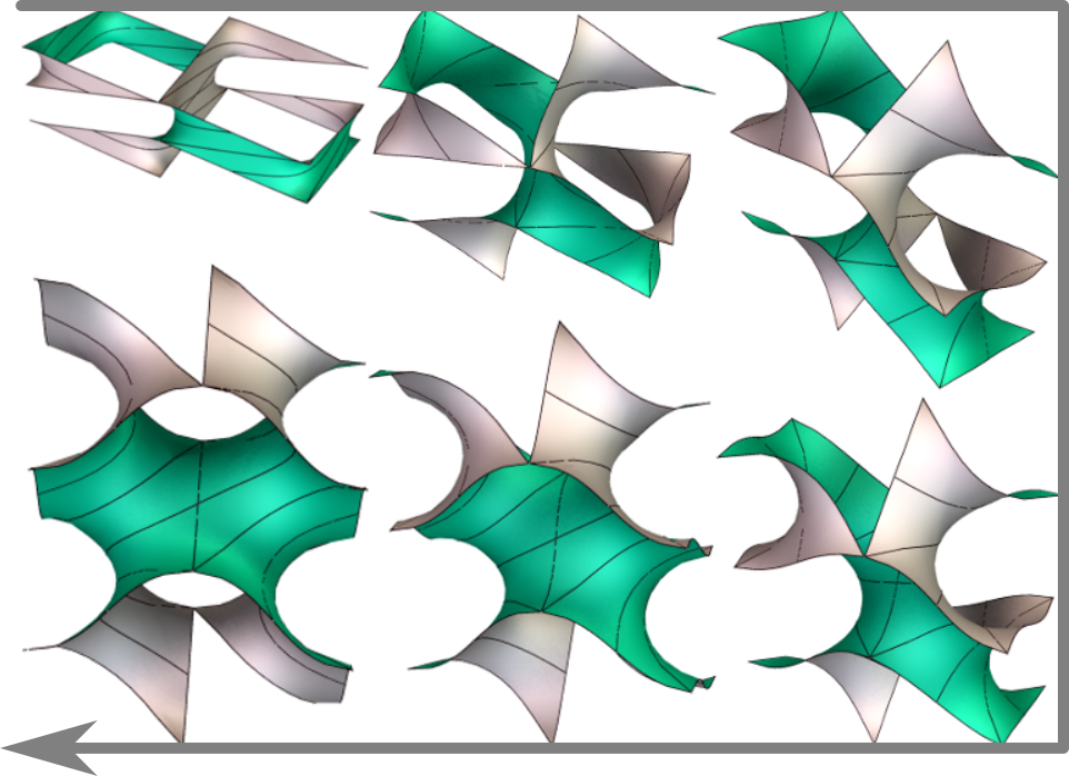
Figure 10. tG surfaces with $\operatorname{Re}\tau=-0.95$, $-0.6$, $-0.2$, $0.2$, $0.6$ and $0.95$, in the indicated order.

5.2. rGL family

In picture 8, we show for $\mathcal{R}$ the numerical solutions to (3) with $-1<\operatorname{Re}\tau<1/2$. The two half-circle represents an order-3 analogue of the CLP surface, termed hCLP in [LL90], but already known to Schwarz [Sch90]; see also [FH92, EFS15] . Surfaces in hCLP are not embedded, but also not dense in the space. It is very easy to visualize and behaves very much like CLP. In particular, it’s Weierstrass data is as shown in Figure 12; compare CLP in Table 1.

Our task is to prove the existence of the continuous 1-parameter solution curve that we see in the picture, which we call the rGL family. Let the shaded domain in the figure be denoted by

$$\Omega_{r}=\{\tau\mid\operatorname{Im}\tau>0,-1<\operatorname{Re}\tau<1/2,|\tau\pm 1/2|>1/2\}.$$

Figure 11. Solutions for $\mathcal{R}$ to (3) with $-1<\operatorname{Re}\tau<1/2$.

Figure 12. Weierstrass data for hCLP.

Proposition 5.2.

There exists a continuous 1-dimensional curve of $\tau$ in $\Omega_{r}$ that solves (3). This curve tends to $-1$ at one end and to $1/2+ti$ for some $0<t<\infty$ at the other end. Moreover, the triply periodic minimal surfaces of genus three represented by points on the curve are all embedded.

Proof.

Part of the proof is very similar to tG, so we just provide a sketch.

The line $\operatorname{Re}\tau=-1$ corresponds to the H family, and we have $\theta_{h}=\pi/2>\theta_{v}$.

The half-circle $|\tau+1/2|=1/2$ corresponds to the hCLP family, and we have $\theta_{h}<\theta_{v}$.

The line $\operatorname{Re}\tau=1/2$ correspond to the rPD family, and we have $\theta_{h}=\theta_{v}=0$. This solves the period condition, but not helpful for us.

As $\operatorname{Im}\tau\to\infty$, we have $\theta_{h}\to\operatorname{Re}(1/2-\tau)\pi/3>\theta_{v}=0$. The argument for the asymptotic behavior is very similar as in the proof of Lemma A.2, so we will not repeat it.

By the same argument as for tG, we conclude that $\theta_{h}>\theta_{v}$ for $\tau=1/2-\epsilon+i\eta$ as long as $\eta>H$ and $\epsilon<\delta$ for some positive constants $H$ and $\delta$.

More care is however needed on the half-circle $|\tau-1/2|=1/2$. It corresponds again to the hCLP family. When $dh=\exp(-i\arg\tau)dz$, the image of $\tau/2$ is directly above the image of $0$. In this case, we know very well that the flat structure of $\Phi_{1}$ is as depicted in Figure 13. We see that

$$\arg\int_{0}^{(1+\tau)/2}dh\cdot G=\arg\int_{0}^{(1+\tau)/2}dz\cdot G\exp(-i\arg\tau)=\theta_{h}-\arg\tau<0.$$

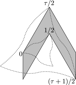
Figure 13. Image of the rectangle with vertices at $0$, $1/2-\tau/2$, $1/2+\tau/2$, $\tau$, under the map $\Phi_{1}$ for an hCLP surface (the grey area). The twisted triangular annulus is sketched (exaggeratedly) in dashed curves.

Let $a$ denote the length of the tilted segments (e.g. from $0$ to $\tau/2$) in the flat structure, and $b$ the length of the vertical segments (e.g. from $1/2$ to $\tau/2$). If follows from an extremal length argument that the ratio $a/b$ increases monotonically as $\tau$ travels along the half-circle with increasing $\operatorname{Re}\tau$. Then we see that $\theta_{h}-\arg\tau$ increases monotonically from $-\pi/2$ to $0$.

On the other hand, it follows from elementary geometry that $\theta_{v}-\arg\tau=\arg\tau-\pi/2$, which decreases monotonically as $\tau$ travels along the half-circle with increasing $\operatorname{Re}\tau$. Consequently, there is a unique $\tau$ on the half-circle for which $\theta_{v}=\theta_{h}$, and we know very well that this occurs at $\tau=(1+i)/2$. At this point, it is interesting to verify that $a=b$, hence $\theta_{h}-\arg\tau=-\pi/4=-\arg\tau$.

Therefore, by monotonicity, we have $\theta_{h}<\theta_{v}$ on the left quarter of this half-circle.

We then conclude the existence of a continuous curve of $\tau$, namely the rG family, that solves $\theta_{h}=\theta_{v}$ and separates the half-circles $|\tau\pm 1/2|=1/2$ from the line $\operatorname{Re}\tau=-1$ and the infinity. This curve must tend to the common limit of hCLP and H (a saddle tower of order 3 at $\tau\to-1$) and intersect rPD at a finite point.

Moreover, the Lidinoid and the gyroid are the unique solutions on their respective vertical lines. Hence the rGL family must contain them both. Their embeddedness then ensures the embeddedness of all TPMSg3s in the rGL family. ∎

In Figure 14, we show two adjacent ribbons for some rGL surfaces. They form a fundamental unit for the translational symmetry group.

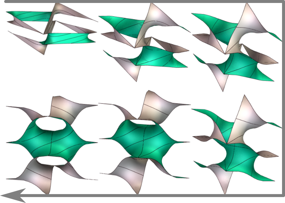
Figure 14. rGL surfaces with $\operatorname{Re}\tau=-0.95$, $-0.7$, $-0.4$, $-0.1$, $0.2$ and $0.45$, in the indicated order.

6. Discussion

6.1. Bifurcation

A TPMSg3 is a bifurcation instance if the same deformation of its lattice could lead to different deformations (bifurcation branches) of the surface. Both the tG–tD and the rGL–rPD intersections are bifurcation instances.

Bifurcation instances among classical TPMSg3s are systematically investigated in [KPS14], but some of them had no explicit bifurcation branch at the time. Two bifurcation instances were discovered in tD [KPS14]. The recently discovered t$\Delta$ family provides the missing bifurcation branch to one of them [CW18a]. The other bifurcation instance seems to escape the attention. Its conjugate is identified as the tP surface obtained from the square catenoid of maximum height, but no bifurcation branch was previously known for itself. Numerics from [KPS14] and [FH99] (see also [STFH06]), which we can confirm with the help of (6) in Appendix, shows that this is exactly the tG–tD intersection with $\tau\approx 1+1.51019i$. Hence tG provides the missing bifurcation branch.

Likewise, two bifurcation instances were discovered in rPD [KPS14]. One of them is identified as the rPD surface obtained from the triangular catenoid of maximum height. The other is its conjugate, for which no bifurcation branch was previously known. Numerics from [KPS14] and [FH99] (see also [STFH06]) shows that this is exactly the rGL–rPD intersection, hence rGL provides the missing bifurcation branch.

Therefore, all bifurcation instances discovered in [KPS14] have now an explicit bifurcation branch.

Remark 6.1.

Curiously, both tG–tD and rGL–rPD intersections are conjugate to catenoids of maximum height. Numerics shows that the height of the twisted catenoid seems to increase monotonically with $\operatorname{Re}\tau$ along the tG and rGL families, and reaches the maximum at the intersection.

6.2. Reflection group

In this part, we point out that “reflections in classical TPMSg3 families” generate a reflection group that acts on $\mathcal{T}$ and $\mathcal{R}$.

We have seen that each $\tau$ corresponds to a marked twisted catenoid. The marked square catenoid is invariant under $\tau\mapsto\tau+4$, and the marked triangular catenoid is invariant under $\tau\mapsto\tau+3$.

For a twisted square catenoid, as one increases $\operatorname{Re}\tau$ beyond $1$, the twist angle increases beyond $\pi$. However, note that $\tau\mapsto 2-\tau$ only results in a reflection of the marked catenoid. Consequently, their associate surfaces with the same associate angle differ only by handedness. So, if $\tau$ closes the period with associate angle $\theta$ and gives an embedded TPMSg3 in $\mathcal{T}$, then $2-\tau$ gives the same TPMSg3 with the same associate angle. Similarly, one can decrease $\operatorname{Re}\tau$ below $-1$, but $\tau\mapsto-2-\tau$ only results in a reflection, hence $\tau$ and $-2-\tau$ gives the same TPMSg3 in $\mathcal{T}$.

So we have shown that $\mathcal{T}$ is invariant under the reflections in the vertical lines $\operatorname{Re}\tau=\pm 1$ (tP and tD). The same argument applies to show that $\mathcal{R}$ is invariant under the reflections in $\operatorname{Re}\tau=-1$ (H) and $\operatorname{Re}\tau=1/2$ (rPD).

Now let us apply the transform $\tau^{\prime}=1/\bar{\tau}$, which exchanges the vertical lines $\operatorname{Re}\tau=\pm 1$ with the half-circles $|\tau\pm 1/2|=1/2$. Then Figure 8 becomes Figure 15.

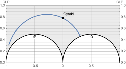
Figure 15. Transform of Figure 8 under the inversion $\tau^{\prime}=1/\bar{\tau}$.

The vertical lines $\operatorname{Re}\tau^{\prime}=\pm 1$ correspond to CLP surfaces. With such a $\tau^{\prime}$ and associate angle $\pi/2$, we know very well that the strip $0<\operatorname{Im}z<\operatorname{Im}\tau^{\prime}/2$ is mapped by the Weierstrass parameterization to a minimal strip bounded by two periodic zig-zag polygonal curves related by a vertical translation. Each polygonal curve consists of segments of equal length, making $\pi/2$ angles in alternating directions.

As we increase $\operatorname{Re}\tau^{\prime}$, the straight segments of the polygonal curves become symmetric curves. At the same time, the two boundaries begin to drift with respect to each other. When $\operatorname{Re}\tau^{\prime}=0$, the drift is exactly half of a period, then reflectional symmetry is restored and the segments become straight again; this is a tD surface. When $\operatorname{Re}\tau^{\prime}=1$, the drift is exactly one period, and a CLP surface is restored.

In principle, we could have built the whole paper on “drifted strips” instead of “twisted catenoids”. We will not go too far in this direction. Nevertheless, the alternative view facilitates the following observation: the transforms $\tau^{\prime}\mapsto 2-\tau^{\prime}$ and $\tau^{\prime}\mapsto-2-\tau^{\prime}$ only result in a reflection of the drifted strip. Consequently, $\mathcal{T}$ is invariant under the reflections in $\operatorname{Re}\tau^{\prime}=\pm 1$ (CLP). Similarly, $\mathcal{R}$ is invariant under the reflections in hCLP families ($\operatorname{Re}\tau^{\prime}=\pm 1$).

If we parameterize $\mathcal{T}$ and $\mathcal{R}$ by $\tau$ in the upper half-plane, which can be seen as the hyperbolic space, then we have proved that

Proposition 6.2.

• $\mathcal{T}$ is invariant under the discrete group generated by reflections in $\operatorname{Re}\tau=-1$ (tP), $\operatorname{Re}\tau=1$ (tD) and $|\tau\pm 1/2|=1/2$ (CLP).

• $\mathcal{R}$ is invariant under the discrete group generated by reflections in $\operatorname{Re}\tau=-1$ (H), $\operatorname{Re}\tau=1/2$ (rPD) and $|\tau\pm 1/2|=1/2$ (hCLP).

6.3. Higher pitch

We have seen that a tG surface consists of ribbons bounded by helices, and the pitch of the helices doubles the vertical distance between them. In general, for any surface in $\mathcal{T}$ and $\mathcal{R}$, the ratio of the pitch of the helices to the vertical distance between them must be an even integer, say $2p$; we call $p$ the pitch of the surface. The vertical associate angle for a surface of pitch $p$ is $\theta_{v}(\tau;p)=\arg(\tau+1-2/p)-\pi/2$ for $\mathcal{T}$, and $\theta_{v}(\tau;p)=\arg(\tau+1-3/2p)-\pi/2$ for $\mathcal{R}$. The period condition is again $\theta_{h}(\tau)=\theta_{v}(\tau;p)$.

It is immediate that $p=0$ for tP. We have seen that tD and tG close the period with $p=1$. It is also not difficult to see that CLP closes the period with $p=2$. In this case, a catenoid and the one directly above it opens into two ribbons that occupy the same vertical cylinder. They interlace each other, and the vertical gap between them equals the vertical width of each single ribbon, allowing adjacent ribbons to fit exactly in.

More generally, for a surface of pitch $p$, $p$ ribbons occupy the same vertical cylinder so that adjacent ribbons fit exactly in. When $p\equiv 0\pmod{2}$, one easily verifies that the half-circle $|\tau+1-1/p|=1/p$ closes the period for $\mathcal{T}$ surfaces with pitch $p$. By the reflection group, we see that this half-circle corresponds to tP if $p\equiv 0\pmod{4}$ and to CLP if $p\equiv 2\pmod{4}$. We now prove that

Lemma 6.3.

Let

$$\tau^{\prime}=-\frac{(2k-1)\bar{\tau}+(2k-2)}{2k\bar{\tau}+(2k-1)}$$

be the image of $\tau$ under the reflection in the half-circle $|\tau+1-1/2k|=1/2k$. If $\tau$ closes the period (for $\mathcal{T}$ or $\mathcal{R}$) with pitch $p$, then $\tau^{\prime}$ closes the period with pitch $q=4k-p$.

Proof.

Note that $2/q-1$ and $2/p-1$ are related by the reflection in the named half-circle. It then follows from elementary geometry that $\theta_{v}(\tau;p)+\theta_{v}(\tau^{\prime};q)=\arg(\tau+1-1/2k)$. On the other hand, note that

$$\tau^{\prime}+1=\frac{\bar{\tau}+1}{2k\bar{\tau}+(2k-1)}.$$

Then a change of variable in the integration $\psi(\tau)$ shows that $\theta_{h}(\tau)+\theta_{h}(\tau^{\prime})=-\arg(2k\bar{\tau}+(2k-1))=\arg(\tau+1-1/2k)$. So $\theta_{h}(\tau)=\theta_{v}(\tau;p)$ implies that $\theta_{h}(\tau^{\prime})=\theta_{v}(\tau^{\prime};q)$. ∎

In particular, by reflections in CLP (resp. hCLP), we see that tG and tD (resp. rGL and rPD) close the period for each $p\equiv 1\pmod{2}$.

6.4. Uniqueness

We conjecture the following uniqueness statements.

Conjecture 6.4.

• For every $r\in(-1,1)$, there is a unique $\tau$ with $\operatorname{Re}\tau=r$ that solves the period condition (3) for $\mathcal{T}$ with pitch $1$.

• For every $r\in(-1,1/2)$, there is a unique $\tau$ with $\operatorname{Re}\tau=r$ that solves the period condition (3) for $\mathcal{R}$ with pitch $1$.

The uniqueness has been proved by Weyhaupt [Wey06] for $\mathcal{T}$ with $\Re\tau=0$ (gyroid) and for $\mathcal{R}$ with $\Re\tau=-1/2$ (gyroid) and $0$ (Lidinoid). This shows that

Theorem 6.5.

The gyroid and the Lidinoid are the only non-trivial embedded TPMSg3s in the associate families of tP, tD, rPD and H surfaces.

Proof.

Any other embedded TPMSg3 must, by construction, lie on the same vertical lines, hence contradict the uniqueness. ∎

Our approach leads to a simple proof that works not only for the gyroid and the Lidinoid but also for the tG surfaces with $\operatorname{Re}\tau=\pm 1/2$. Here is a sketch: On the one hand, it is immediate that $\theta_{v}$ decreases monotonically with $\operatorname{Im}\tau$. On the other hand, by enlarging the outer square or triangle, and shrinking the inner square or triangle, one easily sees from the flat structure that $\theta_{h}$ increases monotonically with $\operatorname{Im}\tau$. This simple proof is possible because, for these cases, the twist angles take special values and do not vary with $\operatorname{Im}\tau$. This may not hold for other cases, for which even the meaning of “twist angle” is not clear.

We also conjecture the following classification statement.

Conjecture 6.6.

• The tP, tD, CLP and tG surfaces are the only members of $\mathcal{T}$.

• The H, rPD and rGL surfaces are the only members of $\mathcal{R}$.

For a proof, we need to prove the previous conjecture first, then also exclude the existence of new surface with pitch $0$ or $2$.

Moreover, note that the order-2 rotations around horizontal axes are only used to determine the López–Ros factor. We wonder if this is necessary and conjecture that

Conjecture 6.7.

• The tP, tD, CLP and tG surfaces are the only TPMSg3s with an order-4 screw symmetry.

• The H, rPD and rGL surfaces are the only TPMSg3s with an order-3 screw symmetry.

Appendix A Asymptotic behavior of associate angle

We now give a detailed asymptotic analysis of $\theta_{h}$ for $\mathcal{T}$.

We need to study the shape of the twisted square annulus with more care. For safety and convenience, we adopt the natural convention (see Section 3.4) for all computations involving Jacobi elliptic functions. So we define $\tilde{\tau}=\tau-r$ where $r:=\lfloor\operatorname{Re}\tau+1/2\rfloor$, hence $-1/2<\operatorname{Re}\tilde{\tau}\leq 1/2$. We write $\tilde{m}=\lambda(2\tilde{\tau})$, and correspondingly $\tilde{K}=K(\tilde{m})$ and $\tilde{K}^{\prime}=-2i\tilde{\tau}\tilde{K}$. Note that $\tilde{K}^{\prime}=K(1-\tilde{m})$ coincides with the usual definition of the associated complete elliptic integral of the first kind.

Remark A.1.

The arguments of the Jacobi elliptic functions can be directly replaced by their tilde versions. This practice is however not safe elsewhere. In particular, the López–Ros factor $m^{1/4}$ can not be directly replaced by $\tilde{m}^{1/4}$. Instead, we must use the convention that

$$\arg m=2\pi r+\arg\tilde{m}.$$

Let us first look at

$$\psi_{1}(\tau):=\int_{0}^{1/2}(m^{1/4}\operatorname{sn}(4\tilde{K}z;\tilde{\tau}))^{1/2}dz,$$

which is a vector pointing from $\Phi_{1}(0)$ to $\Phi_{1}(1/2)$, hence an straightened edge vector of the inner twisted square. With the change of variable $\zeta=\operatorname{sn}(4\tilde{K}z;\tilde{\tau})$, we have

(4) $$\psi_{1}(\tau)=2\frac{m^{1/8}}{4\tilde{K}}\int_{0}^{1}\frac{\zeta^{1/2}d\zeta}{\sqrt{(1-\zeta^{2})(1-\tilde{m}\zeta^{2})}}.$$

Here we used the identities

$$\frac{d}{dz}\operatorname{sn}(z;\tilde{\tau}) =\operatorname{cn}(z;\tilde{\tau})\operatorname{dn}(z;\tilde{\tau});$$

$$\operatorname{cn}^{2}(z;\tilde{\tau}) =1-\operatorname{sn}^{2}(z;\tilde{\tau});$$

$$\operatorname{dn}^{2}(z;\tilde{\tau}) =1-\tilde{m}\operatorname{sn}^{2}(z;\tilde{\tau}).$$

Then we compute the integral

$$\psi_{2}(\tau):= \int_{0}^{\tilde{\tau}/2}(m^{1/4}\operatorname{sn}(4\tilde{K}z;\tilde{\tau}))^{1/2}dz,$$

$$= \int_{0}^{1/2}(m^{1/4}\operatorname{sn}(4\tilde{K}\tilde{\tau}x;\tilde{\tau}))^{1/2}\tilde{\tau}dx$$

$$= \int_{0}^{1/2}(m^{1/4}\operatorname{sn}(2i\tilde{K}^{\prime}x;\tilde{\tau}))^{1/2}\tilde{\tau}dx.$$

This is a vector pointing from $\Phi_{1}(0)$ to $\Phi_{1}(\tilde{\tau}/2)$, hence from an inner vertex to the nearest outer vertex of the twisted annulus. Then we use the Jacobi imaginary transformation $\operatorname{sn}(z;\tau)=-i\operatorname{sc}(iz;-1/\tau)$ and obtain

$$\psi_{2}(\tau)= \int_{0}^{1/2}(-im^{1/4}\operatorname{sc}(-2\tilde{K}^{\prime}x;-1/\tilde{\tau}))^{1/2}\tilde{\tau}dx$$

(5) $$= e^{3\pi i/4}\frac{m^{1/8}}{4\tilde{K}}\int_{0}^{\infty}\frac{\xi^{1/2}d\xi}{\sqrt{(1+\xi^{2})(1+\tilde{m}\xi^{2})}},$$

where we changed the variable $\xi=-\operatorname{sc}(-2\tilde{K}^{\prime}x;-1/\tilde{\tau})$ and used the identities

$$\frac{d}{dz}\operatorname{sc}(z;\tilde{\tau}) =\operatorname{dc}(z;\tilde{\tau})\operatorname{nc}(z;\tilde{\tau});$$

$$\operatorname{dc}^{2}(z;\tilde{\tau}) =1+(1-\tilde{m})\operatorname{sc}^{2}(z;\tilde{\tau});$$

$$\operatorname{nc}^{2}(z;\tilde{\tau}) =1+\operatorname{sc}^{2}(z;\tilde{\tau}).$$

The two vectors $\psi_{1}(\tau)$ and $\psi_{2}(\tau)$ can determine the images of all branch points under $\Phi_{1}$.

Lemma A.2.

$\theta_{h}(\tau)\to\operatorname{Re}(1-\tau)\pi/4$ as $\operatorname{Im}\tau\to\infty$.

Proof.

As $\operatorname{Im}\tau=\operatorname{Im}\tilde{\tau}\to\infty$, we have [Law89, (2.1.12)]

$$m(\tau)=\lambda(2\tau)\sim 16\exp(2i\pi\tau),$$

so $|m|\to 0$. Recall that $\tilde{K}(0)=\pi/2$, and that the integral in (4) tends to

$$\int_{0}^{1}\frac{\zeta^{1/2}d\zeta}{\sqrt{(1-\zeta^{2})}}$$

which is bounded. Therefore, $\psi_{1}(\tau)\to 0$ as $\operatorname{Im}\tau\to\infty$. In other words, the size of the inner square tends to $0$.

On the other hand, we have

$$\psi_{2}(\tau)\sim e^{3i\pi/4}\frac{m^{1/8}}{4\tilde{K}}\int_{0}^{\infty}\frac{d\xi}{\xi^{1/2}\sqrt{1+\tilde{m}\xi^{2}}}=e^{(r+3)i\pi/4}\frac{\tilde{m}^{-1/8}}{4\tilde{K}}\int_{0}^{\infty}\frac{du}{u^{1/2}\sqrt{1+u^{2}}},$$

where we changed the variable $u=\xi\sqrt{m}$ and used the convention that $\arg m=2\pi r+\arg\tilde{m}$. Note again that the integral is bounded, hence $|\psi_{2}(\tau)|\sim|m|^{-1/8}$. In other words, the size of the outer square grows exponentially with $\operatorname{Im}\tilde{\tau}$.

Therefore, as $\operatorname{Im}\tau\to\infty$, the integral

$$\psi(\tau)=\int_{0}^{(1+\tau)/2}(m^{1/4}\operatorname{sn}(4Kz;\tau))^{1/2}dz$$

is dominated by

$$\psi(\tau)\sim \int_{(r+1)/2}^{(\tau+1)/2}(m^{1/4}\operatorname{sn}(4Kz;\tau))^{1/2}dz\sim e^{-(r+1)i\pi/2}\psi_{2}(\tau)$$

$$\sim e^{-(r+1)i\pi/2}e^{(r+3)i\pi/4}\frac{\tilde{m}^{-1/8}}{4\tilde{K}}\int_{0}^{\infty}\frac{du}{u^{1/2}\sqrt{1+u^{2}}},$$

Now we can conclude that

$$\theta_{h}(\tau)=\arg\psi(\tau)\to(1-r-\operatorname{Re}\tilde{\tau})\pi/4=\operatorname{Re}(1-\tau)\pi/4.$$

∎

A similar argument applies to rGL, so we omit the proof. The conclusion is that

$$\theta_{h}\to\operatorname{Re}(1/2-\tau)\pi/3\quad\text{as $\operatorname{Im}\tau\to\infty$.}$$

Lemma A.3.

$\theta_{h}(\tau)\to 0$ from the negative side as $\tau\to 1$ within $\Omega_{t}$.

Proof.

By the transformation $\lambda(-1/\tau)=1-\lambda(\tau)$ [Law89, (9.4.10)], we see that

$$\tilde{m}=m(\tilde{\tau})=1-16e^{-i\pi/2\tilde{\tau}}+O(e^{-i\pi/\tilde{\tau}})\qquad\text{as }\tilde{\tau}\to 0.$$

Then [Law89, Exercise 8.13]

$$\tilde{K}=\int_{0}^{1}\frac{d\zeta}{\sqrt{(1-\zeta^{2})(1-\tilde{m}\zeta^{2})}}\sim-\frac{1}{2}\ln(1-\tilde{m})\sim\frac{i\pi}{4\tilde{\tau}}.$$

The standard proof for this also applies to prove that the integral in (4) satisfies

$$\int_{0}^{1}\frac{\zeta^{1/2}d\zeta}{\sqrt{(1-\zeta^{2})(1-\tilde{m}\zeta^{2})}}\sim-\frac{1}{2}\ln(1-\tilde{m})\sim\frac{i\pi}{4\tilde{\tau}}.$$

One can also quickly convince oneself by noting that the integrand in (4) differs from the integrand of $\tilde{K}$ only by a factor $\zeta^{1/2}$, which can be neglected near $1$, where the divergence occurs. In other words, the integral in (4) is asymptotically equivalent to $\tilde{K}$. So we have $\psi_{1}(\tau)\to\frac{1}{2}m^{1/8}$ as $\tau\to 1$.

On the other hand, the integral in (5) tends to

$$\int_{0}^{\infty}\frac{\xi^{1/2}d\xi}{1+\xi^{2}}=\frac{\pi}{\sqrt{2}}$$

which is bounded, hence $\psi_{2}(\tau)\to 0$. Therefore, as $\tau\to 1$, we see from the flat structure that $\psi(\tau)\to\frac{1-i}{2}m^{1/8}$, so

$$\theta_{h}(\tau)=\arg(m(\tau))/8-\pi/4=\arg(\tilde{m})/8\to 0.$$

Note again that we used the convention $\arg m(\tau)=m(\tilde{\tau}+1)=2\pi+\arg m(\tilde{\tau})$.

We now prove that the convergence is from the negative side. A routine calculation shows that

$$\arg(e^{-i\pi/2\tilde{\tau}})=-\frac{\pi\operatorname{Re}\tilde{\tau}}{2|\tilde{\tau}|^{2}}=\frac{\pi\sin\theta_{v}}{2|\tilde{\tau}|}.$$

When $\tau\in\Omega_{t}$, it follows from elementary geometry that $0<\sin\theta_{v}<|\tilde{\tau}|$, hence $0<\arg(e^{-i\pi/2\tilde{\tau}})<\pi/2$. Therefore, when $\tau$ tends to $0$ within $\Omega_{t}$, we have $\arg(\tilde{m})=\arg(1-16e^{-i\pi/2\tilde{\tau}})<0$. ∎

Remark A.4.

The integrals arisen from $\mathcal{T}$ surfaces (e.g. (4) and (5)) can be explicitly expressed in terms of elliptic integrals; see [Bow61, Chapter X] and [BF71, §595 et seq.]. For example, we have

$$\int_{0}^{1/2}(m^{1/4}\operatorname{sn}(4\tilde{K}z;\tilde{\tau}))^{1/2}dz= \frac{e^{r\pi i/4}}{2\sqrt{2}}\frac{\tilde{m}^{-1/8}}{\sqrt{1+\tilde{m}^{1/2}}}\frac{K(\mu)-K^{\prime}(\mu)}{K(\tilde{m})},$$

$$\int_{\tau/2}^{1/2+\tau/2}(m^{1/4}\operatorname{sn}(4\tilde{K}z;\tilde{\tau}))^{1/2}dz= \frac{e^{r\pi i/4}}{2\sqrt{2}}\frac{\tilde{m}^{-1/8}}{\sqrt{1+\tilde{m}^{1/2}}}\frac{K(\mu)+K^{\prime}(\mu)}{K(\tilde{m})},$$

for the inner and outer edge vectors of the twisted annulus, where

$$\mu=\frac{(1+\tilde{m}^{1/4})^{2}}{2+2\tilde{m}^{1/2}}.$$

We then obtain that

(6) $$\psi(\tau)=e^{r\pi i/4}\frac{1-i}{2\sqrt{2}}\frac{\tilde{m}^{-1/8}}{\sqrt{1+\tilde{m}^{1/2}}}\frac{K(\mu)}{K(\tilde{m})}.$$

This facilitates the numeric calculation for the tG–tD intersection but does not give an explicit expression.

We are not aware of equally explicit expressions for integrals arisen from $\mathcal{R}$ surfaces.

References

- [BB98] Jonathan M. Borwein and Peter B. Borwein. Pi and the AGM, volume 4 of Canadian Mathematical Society Series of Monographs and Advanced Texts. John Wiley & Sons, Inc., New York, 1998. A study in analytic number theory and computational complexity, Reprint of the 1987 original, A Wiley-Interscience Publication.
- [BF71] Paul F. Byrd and Morris D. Friedman. Handbook of elliptic integrals for engineers and scientists. Die Grundlehren der mathematischen Wissenschaften, Band 67. Springer-Verlag, New York-Heidelberg, 1971. Second edition, revised.
- [Bow61] F. Bowman. Introduction to elliptic functions with applications. Dover Publications, Inc., New York, 1961.
- [CW18a] Hao Chen and Matthias Weber. A new deformation family of Schwarz’ D surface. page 15 pp., 2018. Preprint, arXiv:1804.01442.
- [CW18b] Hao Chen and Matthias Weber. An orthorhombic deformation family of Schwarz’ H surfaces. page 17 pp., 2018. Preprint, arXiv:1807.10631.
- [DLMF] NIST Digital Library of Mathematical Functions. http://dlmf.nist.gov/, Release 1.0.19 of 2018-06-22. F. W. J. Olver, A. B. Olde Daalhuis, D. W. Lozier, B. I. Schneider, R. F. Boisvert, C. W. Clark, B. R. Miller and B. V. Saunders, eds.
- [EFS15] Norio Ejiri, Shoichi Fujimori, and Toshihiro Shoda. A remark on limits of triply periodic minimal surfaces of genus 3. Topology Appl., 196(part B):880–903, 2015.
- [FH92] Andrew Fogden and Stephen T Hyde. Parametrization of triply periodic minimal surfaces. II. regular class solutions. Acta Crystallographica Section A, 48(4):575–591, 1992.
- [FH99] Andrew Fogden and Stephan T. Hyde. Continuous transformations of cubic minimal surfaces. The European Physical Journal B-Condensed Matter and Complex Systems, 7(1):91–104, 1999.
- [FHL93] Andrew Fogden, M. Haeberlein, and Sven Lidin. Generalizations of the gyroid surface. J. Phys. I, 3(12):2371–2385, 1993.
- [FK92] H. M. Farkas and I. Kra. Riemann surfaces, volume 71 of Graduate Texts in Mathematics. Springer-Verlag, New York, second edition, 1992.
- [FW09] Shoichi Fujimori and Matthias Weber. Triply periodic minimal surfaces bounded by vertical symmetry planes. Manuscripta Math., 129(1):29–53, 2009.
- [GBW96] Karsten Große-Brauckmann and Meinhard Wohlgemuth. The gyroid is embedded and has constant mean curvature companions. Calc. Var. Partial Differential Equations, 4(6):499–523, 1996.
- [Hur32] Adolf Hurwitz. Über algebraische Gebilde mit eindeutigen Transformationen in sich, pages 391–430. Springer Basel, Basel, 1932.
- [Kar89] Hermann Karcher. The triply periodic minimal surfaces of Alan Schoen and their constant mean curvature companions. Manuscripta Math., 64(3):291–357, 1989.
- [KK79] Akikazu Kuribayashi and Kaname Komiya. On Weierstrass points and automorphisms of curves of genus three. In Algebraic geometry (Proc. Summer Meeting, Univ. Copenhagen, Copenhagen, 1978), volume 732 of Lecture Notes in Math., pages 253–299. Springer, Berlin, 1979.
- [KPS14] Miyuki Koiso, Paolo Piccione, and Toshihiro Shoda. On bifurcation and local rigidity of triply periodic minimal surfaces in . page 26 pp., 2014. Preprint, arXiv:1408.0953, to appear in Annales de l’Institut Fourier.
- [KWH93] Hermann Karcher, Fu Sheng Wei, and David Hoffman. The genus one helicoid and the minimal surfaces that led to its discovery. In Global analysis in modern mathematics (Orono, ME, 1991; Waltham, MA, 1992), pages 119–170. Publish or Perish, Houston, TX, 1993.
- [Law89] Derek F. Lawden. Elliptic functions and applications, volume 80 of Applied Mathematical Sciences. Springer-Verlag, New York, 1989.
- [LL90] Sven Lidin and Stefan Larsson. Bonnet transformation of infinite periodic minimal surfaces with hexagonal symmetry. Journal of the Chemical Society, Faraday Transactions, 86(5):769–775, 1990.
- [LR91] Francisco J. López and Antonio Ros. On embedded complete minimal surfaces of genus zero. J. Differential Geom., 33(1):293–300, 1991.
- [Mee90] William H. Meeks, III. The theory of triply periodic minimal surfaces. Indiana Univ. Math. J., 39(3):877–936, 1990.
- [Oss64] Robert Osserman. Global properties of minimal surfaces in and . Ann. of Math. (2), 80:340–364, 1964.
- [Sch90] Hermann A. Schwarz. Gesammelte Mathematische Abhandlungen, volume 1. Springer, Berlin, 1890.
- [Sch70] Alan H. Schoen. Infinite periodic minimal surfaces without self-intersections. Technical Note D-5541, NASA, Cambridge, Mass., May 1970.
- [STFH06] Gerd E Schröder-Turk, Andrew Fogden, and Stephen T Hyde. Bicontinuous geometries and molecular self-assembly: comparison of local curvature and global packing variations in genus-three cubic, tetragonal and rhombohedral surfaces. The European Physical Journal B-Condensed Matter and Complex Systems, 54(4):509–524, 2006.
- [Wey06] Adam G. Weyhaupt. New families of embedded triply periodic minimal surfaces of genus three in euclidean space. ProQuest LLC, Ann Arbor, MI, 2006. Thesis (Ph.D.)–Indiana University.
- [Wey08] Adam G. Weyhaupt. Deformations of the gyroid and Lidinoid minimal surfaces. Pacific J. Math., 235(1):137–171, 2008.
- [WW98] M. Weber and M. Wolf. Minimal surfaces of least total curvature and moduli spaces of plane polygonal arcs. Geom. Funct. Anal., 8(6):1129–1170, 1998.
- [WW02] Matthias Weber and Michael Wolf. Teichmüller theory and handle addition for minimal surfaces. Ann. of Math. (2), 156(3):713–795, 2002.