A short and sudden increase of the magnetic field strength and the accompanying spectral variability in the O9.7 V star HD 54879

Abstract

Only eleven O-type stars have been confirmed to possess large-scale organized magnetic fields. The presence of a $-600$ G longitudinal magnetic field in the O9.7 V star HD 54879 with a lower limit of the dipole strength of $\sim$2 kG, was discovered a few years ago in the framework of the ESO large program “B-fields in OB stars”. Our FORS 2 spectropolarimetric observations from 2017 October 4 to 2018 February 21 reveal the presence of short and long-term spectral variability and a gradual magnetic field decrease from about $-300$ G down to about $-90$ G. Surprisingly, we discover on the night of 2018 February 17 a sudden, short-term increase of the magnetic field strength and measure a longitudinal magnetic field of $-833$ G. The inspection of the FORS 2 spectrum acquired during the observed magnetic field increase indicates a very strong change in spectral appearance with a significantly lower photospheric temperature and a decrease of the radial velocity by several 10 km s^-1. Different scenarios are discussed in an attempt to interpret our observations. The FORS 2 radial velocity measurements indicate that HD 54879 is a member of a long-period binary.

1 Introduction

The origin of magnetic fields in massive stars is still under debate. It has been argued that magnetic fields could be fossil relics of the fields that were present in the interstellar medium from which the stars have formed (e.g. Moss 2003). This, however, gives no explanation for the low fraction of stars that are found to be magnetic. Different scenarios to explain why only a subclass of early-type stars are observably magnetic in the framework of the fossil field theory were discussed by Borra et al. (1982), who also indicated the need for future hydromagnetic studies, such as dynamo theory and the related problems of magnetic stability. In contrast, the magnetic field in the Sun and stars on the lower main sequence that have outer convection zones or are fully convective is believed to be the result of a dynamo process (e.g. Charbonneau 2014). Though there is no consensus on the exact mechanism, the global rotation and its impact on the convective gas motions are vital for the generation of a large-scale, oscillating magnetic field. The observed rotation-activity relation and the existence of activity cycles support the idea that the magnetic fields of stars on the lower main sequence are dynamo-generated. As the observed field geometries among such stars strongly vary, it is possible that the type of dynamo mechanism is not the same for all stars. Notably, all known mechanisms involve rotating convection.

Cantiello & Braithwaite (2011a) suggested that a subsurface convection zone due to partial ionization in massive stars may be the source of a global magnetic field, winding up toroidally with stochastic buoyancy breakouts at the surface, causing corotating magnetic bright spots at the surface of the star. Dynamos operating in geometrically thin layers have been studied in the context of the solar dynamo, where the overshoot layer below the convection zone has been assumed to be the location of the dynamo. Moss, Tuominen & Brandenburg (1990) reported that the magnetic field geometry produced by such dynamos is generally more complicated than a dipole. The width of the toroidal field belts was found to be about the same as the depth of the overshoot layer and the observed solar butterfly diagram is therefore not correctly reproduced. This finding was confirmed by Rüdiger & Brandenburg (1995), who also pointed out that this type of dynamo produces cycle periods that are substantially shorter than the solar activity cycle period of 22 yr.

Alternatively, magnetic fields in massive stars may be generated by strong binary interaction, i.e. in stellar mergers, or during a mass transfer or common envelope evolution (Tout et al., 2008). In these events, angular momentum surplus creates strong differential rotation in one of the stars (Petrovic et al., 2005) or in the merger product — a key ingredient for the generation of a magnetic field. The binary interaction also leads to enhanced abundances of hydrogen burning products, e.g. nitrogen, at the stellar surface. The number of O-type stars with confirmed magnetic fields detected at a 3$\sigma$-level is currently only eleven (e.g. Grunhut et al. 2017; Schöller et al. 2017), and approximately half of them appear to be nitrogen-rich (e.g. Martins et al. 2012).

The most straightforward explanation for a large scale magnetic field in a massive star is a fossil field, which however would have to be stationary except for a slow decay and have a rather simple geometry. Cyclic activity, on the other hand, requires a large-scale dynamo mechanism. A dynamo could exist in the core, but it is unclear how much the magnetic field generated there could affect the stellar surface and surroundings. A nonaxisymmetric steady field produced by a dynamo in the core could appear to vary with time at the surface if the envelope undergoes cyclic changes. Torsional oscillations could cause a variation of the surface rotation and thus the observed cycle period. However, the torsional oscillations would have to be driven by a force other than the Lorentz force and they would not affect the field strength. MHD simulations of magnetic field generation in the core of A-type stars found rather complex and varying field geometries (Brun, Browning & Toomre, 2005). Because of the comparatively high electric conductivity of the radiative envelope, a magnetic field generated in the core can not reach the surface through diffusion. However, instabilities involving buoyancy or shear could cause the rise of magnetic flux and therefore a variability of the surface magnetic field on a time scale comparable to that of the dynamo. However, the geometry of the surface field would then be much more complicated than a simple dipole. On the other hand, turbulent diffusion will destroy a possible fossil field, which means that a fossil field will be expelled from the core by convection. Featherstone et al. (2009) have studied the interaction between a fossil field and a core dynamo in A-type stars. They found that in the presence of a fossil field the core dynamo can generate stronger fields, thus raising the chance that buoyancy could transport some of the generated magnetic flux to the surface.

Apart from the O9.7 V star HD 54879, all previously studied magnetic O-type stars showed spectral line variability with a period identified as the rotation period. Of the known confirmed eleven magnetic O-type stars, five are associated with the peculiar spectral classification Of?p. This classification was introduced by Walborn (1972) according to the presence of C iii 4650 Å emission with a strength comparable to the neighbouring N iii lines. Such stars are known to exhibit recurrent, and apparently periodic, spectral variations in Balmer, He i, C iii, and Si iii lines, sharp emission or P Cygni profiles in He i and the Balmer lines, and strong C iii emission around 4650 Å. The detection of a magnetic field in HD 54879 was achieved by Castro et al. (2015) using the FOcal Reducer low dispersion Spectrograph (FORS 2; Appenzeller et al. 1998) and the High Accuracy Radial velocity Planet Searcher in polarimetric mode (HARPSpol) in the framework of the ESO Large Prg. 191.D-0255. The authors reported the presence of a $-600$ G longitudinal magnetic field with a lower limit of the dipole strength of $\sim 2$ kG. Magnetospheric parameters of HD 54879 were recently presented by Shenar et al. (2017), who also suggested a rotation period of $\sim 5$ yr. Noteworthy, among the single magnetic O-type stars, HD 54879 has the second strongest magnetic field after the Of?p star NGC 1624-2, for which a dipole strength of $\sim$20 kG was estimated by Wade et al. (2012). The stars HD 54879 and NGC 1624-2 also show the lowest $v\sin i$ values, lower than 8 km s^-1. Current studies of O-type stars indicate that their magnetic fields are dominated by dipolar fields tilted with respect to the rotation axis (the so-called oblique dipole rotator model). Thus, the rotation period is frequently determined from studying the periodicity in the available magnetic data. As of today, an estimation of the rotational periodicity using magnetic field measurements and spectral variability was performed for ten magnetic O-type stars, indicating rotation periods between 7 d for HD 148937 (Naze et al., 2008) and several decades for HD 108 (Naze et al., 2001), while most normal O-type stars have typical rotation periods in the range from 2 to 4 d. In contrast, for HD 54879 only very few magnetic field measurements, three measurements using FORS 2 and three measurements using HARPSpol were available before we started the magnetic field monitoring using FORS 2 observations within the framework of the programme 100.D-0110(A). In the following, we report on our results obtained from the polarimetric observations of HD 54879 carried out using FORS 2 in spectropolarimetric mode.

2 Observations and magnetic field analysis

Table 1: Longitudinal magnetic field values of HD 54879 from FORS 2 data. The S/N is measured at 4800 Å.

MJD	S/N	$\left<B_{\rm z}\right>_{\rm all}$		$\left<B_{\rm z}\right>_{\rm hyd}$		$\left<B_{\rm z}\right>_{\rm N}$
		(G)		(G)		(G)
56696.23411	2360	$-$460$\pm$	65	$-$639$\pm$	121	76$\pm$	66
56697.21621	2400	$-$521$\pm$	62	$-$877$\pm$	91	23$\pm$	63
57099.01501	3060	$-$527$\pm$	45	$-$633$\pm$	65	52$\pm$	45
58030.2744	1700	$-$242$\pm$	120	$-$313$\pm$	158	$-$33$\pm$	107
58031.3448	1870	$-$51$\pm$	86	$-$133$\pm$	117	$-$22$\pm$	70
58033.3604	2160	$-$154$\pm$	74	$-$138$\pm$	118	45$\pm$	68
58035.2867	1710	$-$261$\pm$	83	$-$522$\pm$	139	18$\pm$	77
58036.3591	1780	$-$245$\pm$	65	$-$434$\pm$	129	$-$54$\pm$	73
58041.3450	3130	$-$187$\pm$	57	$-$126$\pm$	91	$-$34$\pm$	55
58043.3604	1660	$-$125$\pm$	55	33$\pm$	94	$-$35$\pm$	55
58046.3496	2080	$-$248$\pm$	86	$-$141$\pm$	152	$-$80$\pm$	76
58049.2865	2290	$-$136$\pm$	62	$-$201$\pm$	117	11$\pm$	59
58051.3598	3970	$-$16$\pm$	82	$-$223$\pm$	104	$-$62$\pm$	90
58062.2035	2240	$-$186$\pm$	55	$-$286$\pm$	98	66$\pm$	58
58073.3423	2410	$-$202$\pm$	52	$-$260$\pm$	81	13$\pm$	56
58098.3371	2090	$-$58$\pm$	53	$-$163$\pm$	113	$-$12$\pm$	58
58099.3109	2300	$-$153$\pm$	66	$-$196$\pm$	104	$-$21$\pm$	62
58100.3289	2010	$-$75$\pm$	78	$-$138$\pm$	124	$-$22$\pm$	72
58103.3134	2640	$-$218$\pm$	52	$-$242$\pm$	105	$-$17$\pm$	54
58149.2310	2240	$-$129$\pm$	54	$-$160$\pm$	98	57$\pm$	53
58150.0603	1740	$-$101$\pm$	62	$-$137$\pm$	122	60$\pm$	63
58151.1108	2380	$-$113$\pm$	60	$-$75$\pm$	101	38$\pm$	56
58152.1369	2950	$-$195$\pm$	57	$-$128$\pm$	102	86$\pm$	69
58154.2698	1370	$-$123$\pm$	99	$-$89$\pm$	128	62$\pm$	96
58161.1319	2080	$-$36$\pm$	56	$-$19$\pm$	116	62$\pm$	75
58162.0188	2200	$-$85$\pm$	59	$-$245$\pm$	112	$-$79$\pm$	63
58164.2586	1500	$-$202$\pm$	132	$-$114$\pm$	166	85$\pm$	158
58166.0420	1130	$-$833$\pm$	118	$-$623$\pm$	155	$-$31$\pm$	166
58170.0332	2390	$-$91$\pm$	49	$-$13$\pm$	94	$-$68$\pm$	53

The 26 new spectropolarimetric observations of HD 54879 with FORS 2 summarized in Table 1 were obtained between 2017 October 4 and 2018 February 21. The first two Columns list the modified Julian dates (MJD) for the middle of the exposure and the signal-to-noise ratio (S/N) of the spectra. We used the GRISM 600B and the narrowest available slit width of 0$\aas@@fstack{\prime\prime}$4 to obtain a spectral resolving power of $R\approx 2000$. The observed spectral range from 3250 to 6215 Å includes all Balmer lines, apart from H$\alpha$, and numerous helium lines. Further, in our observations we used a non-standard readout mode with low gain (200kHz,1$\times$1,low), which provides a broader dynamic range, hence allowing us to reach a higher S/N in the individual spectra. The position angle of the retarder waveplate was changed from $+45^{\circ}$ to $-45^{\circ}$ and vice versa every second exposure, i.e. we have executed the sequence $+45^{\circ}$$-45^{\circ}$$-45^{\circ}$$+45^{\circ}$ four times. Using this sequence of the retarder waveplate ensures an optimum removal of instrumental polarization. The exposure time for the observations of the subexposures $+45^{\circ}$$-45^{\circ}$$-45^{\circ}$$+45^{\circ}$ including overheads, accounted for about 6 min.

A description of the assessment of the presence of a longitudinal magnetic field using FORS 1/2 spectropolarimetric observations was presented in our previous work (e.g. Hubrig et al., 2004a, b, and references therein). Improvements to the methods used, including $V/I$ spectral rectification and clipping, were detailed by Hubrig, Schöller & Kholtygin (2014).

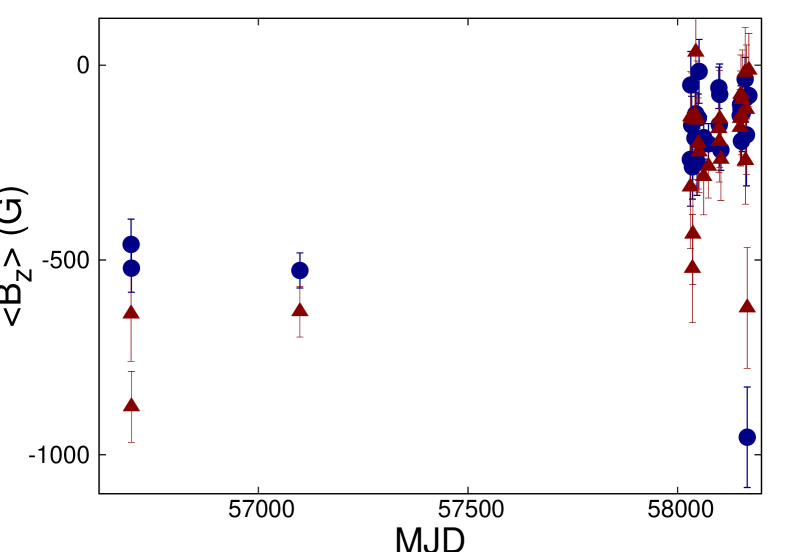
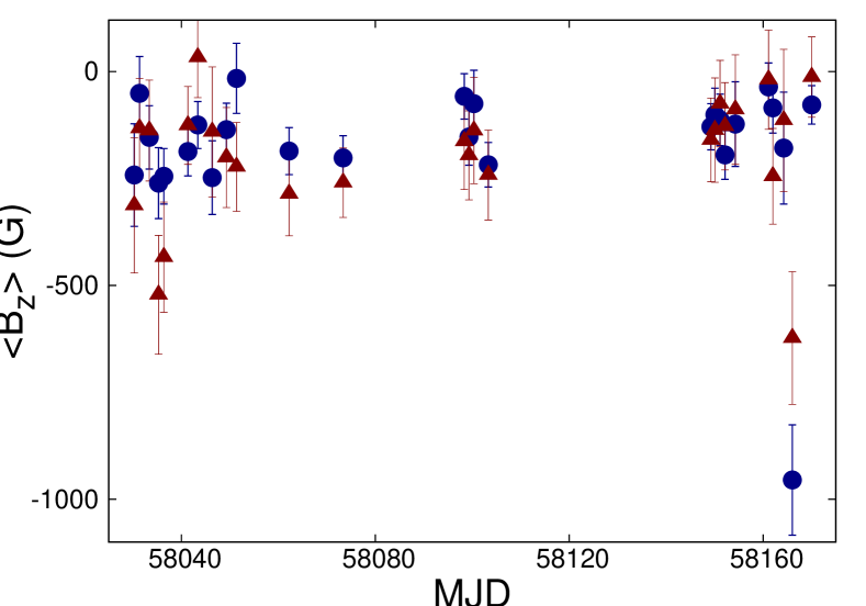
Figure 1: Upper panel: Distribution of the mean longitudinal magnetic field values of HD 54879 using the entire spectrum (blue circles) and those using only the hydrogen lines (red triangles) as a function of MJD between 2014 and 2018. Lower panel: Distribution of the mean longitudinal magnetic field values of HD 54879 as a function of MJD between 2017 and 2018.

The longitudinal magnetic field was measured in two ways: using the entire spectrum including all available lines, or using exclusively hydrogen lines. Furthermore, we have carried out Monte Carlo bootstrapping tests. These are most often applied with the purpose of deriving robust estimates of standard errors (e.g. Steffen et al. 2014). The measurement uncertainties obtained before and after the Monte Carlo bootstrapping tests were found to be in close agreement, indicating the absence of reduction flaws. The results of our magnetic field measurements, those for the entire spectrum or only for the hydrogen lines are presented in Table 1 in Columns 3 and 4, followed by the measurements using all lines in the null spectra. The distribution of the mean longitudinal magnetic field values as a function of MJD is presented in Fig. 1.

Figure 2: Regression analysis of the FORS 2 data of HD 54879 obtained during the night of 2018 February 17 considering the entire spectrum. Left panel: linear fit to Stokes $V$. Middle panel: linear fit to the $N$ spectrum. Right panel: distribution of the longitudinal magnetic field values $P(\left<B_{\rm z}\right>)$, which were obtained via bootstrapping. From the distribution $P(\left<B_{\rm z}\right>)$, we obtain the most likely value for the longitudinal magnetic field $\left<B_{\rm z}\right>=-833\pm 118$ G.

Figure 3: Top: Stokes $I$ profile of He i 5876. Bottom: A typical Zeeman feature in the Stokes $V$ profile of He i 5876 recorded on 2018 February 17.

While the few previous observations in 2014/2015 indicated a longitudinal magnetic field strength of the order of $-$500 G to $-$600 G, our measurements using the observations of HD 54879 carried out from 2017 October 4 to 2018 February 21 show that we approach the rotational phase with the best visibility of the magnetic equator. Over the four and a half months, the magnetic field was gradually decreasing, from $\left<B_{\rm z}\right>\approx-300$ G measured on 2017 October 4 down to $\left<B_{\rm z}\right>\approx-90$ G measured on 2018 February 21. Surprisingly, the observations obtained on 2018 February 17 showed a significant increase of the magnetic field strength, reaching $\left<B_{\rm z}\right>=-833\pm 118$ G in the measurements using the entire spectrum and $\left<B_{\rm z}\right>=-623\pm 155$ G using exclusively the hydrogen lines. In Fig. 2 we present the results of our analysis of the FORS 2 data of HD 54879 obtained during the night of 2018 February 17 considering the entire spectrum. Further, as an example, we present in Fig. 3 a typical Zeeman feature in the Stokes $V$ profile of He i 5876 recorded on 2018 February 17.

Four nights later, on 2018 February 21, the magnetic field strength became again very weak, of the order of $-$90 G. The field decrease observed by us over about 4.5 months suggests that the magnetic/rotation period is rather long, amounting to at least several months, or even years. However, the sudden short-term field strength increase observed on the night of 2018 February 17 (MJD 58166.04) needs a plausible explanation.

3 Spectral changes accompanying the sudden increase of the magnetic field

Järvinen et al. (2017) studied the spectral variability of HD 54879 on different timescales using all available HARPSpol and FORS 2 spectropolarimetric observations obtained between 2014 and 2015. Their analysis of line profiles and radial velocity shifts using HARPSpol and FORS 2 subexposures with different time durations indicated the presence of spectral variability on short timescales, but the degree of this variability was rather low, just at the intensity level of 0.2 per cent and 1.7 per cent, depending on the integration time and the considered element.

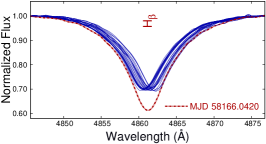
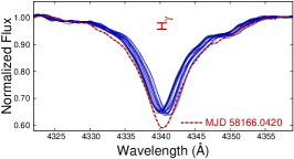
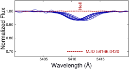
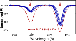
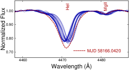
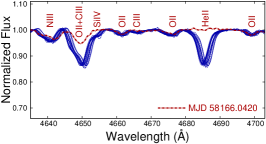
Figure 4: Profile variability of hydrogen, He ii, He i, and metal lines.

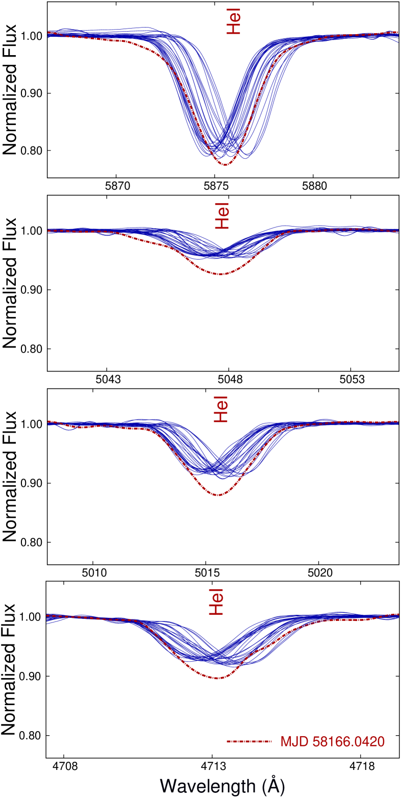
Figure 5: Profile variability of a sample of He i lines.

In Figs. 4 and 5 we present several overplotted spectral lines belonging to different elements observed in FORS 2 spectra acquired from 2014 to 2018. Evidently, all line profiles show distinct radial velocity shifts and very similar profile shapes apart from the line profiles observed at MJD58166.0420 (indicated by the red line) during the sudden increase of the longitudinal magnetic field. At this observing epoch, all absorption hydrogen and He i lines become stronger, whereas higher ionisation lines like He ii, C iii and Si iv turn out to be much weaker, or fully disappear. Also the wind sensitive He ii 4686 line becomes extremely weak. Such a spectral appearance indicates a cooler photospheric temperature at the time of the magnetic field increase.

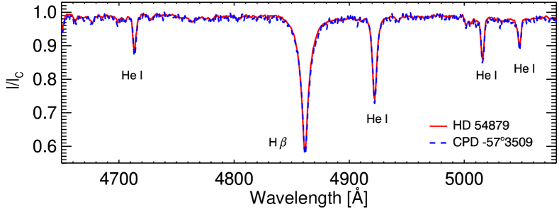
Figure 6: Overplotted He i and hydrogen line profiles of HD 54879 observed on 2018 February 17 and the He-rich star CPD $-$57^∘ 3509 of spectral type B1V.

To estimate the decrease of the photospheric temperature, we compared the spectrum of HD 54879 acquired on 2018 February 17 with a few other early-B type stars well-studied with FORS 2 in the framework of the ESO large program “B-fields in OB stars”. In Fig. 6, we present overplotted He i and hydrogen line profiles of HD 54879 and the He-rich star CPD $-$57^∘ 3509 of spectral type B1 V. The atmospheric parameters of CPD $-$57^∘ 3509, $T_{\rm eff}=23750\,\pm\,250$ K and $\log\,g=4.05\,\pm\,0.10$, were obtained by Przybilla et al. (2016) using a high-resolution high signal-to-noise HARPSpol spectrum. The similarity of both stellar spectra suggests that the spectral type of HD 54879 changed from O9.7 V to B1 V during the night when we observe the sudden magnetic field increase. It is very uncommon that spectral type changes in different rotation phases are observed in massive stars. To our knowledge, only $a$ Cen, a massive star with an anomalous He surface distribution, was reported as a helium-weak star at one extremum of the magnetic field and as helium-rich at the other, indicating B3 and B8 spectral types, respectively (Norris, 1968). However, in that star, the Balmer lines were invariant throughout the He line variation. This is not the case presented here for HD 54879.

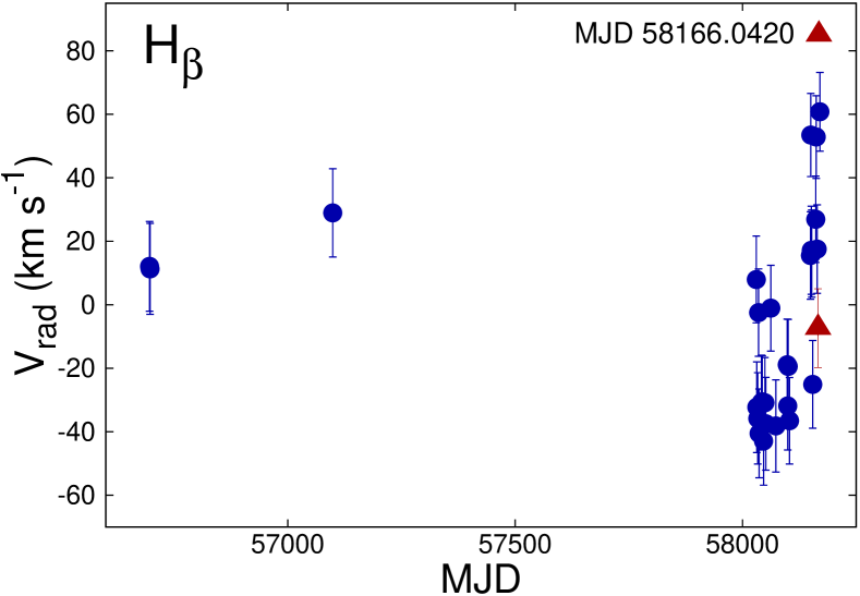
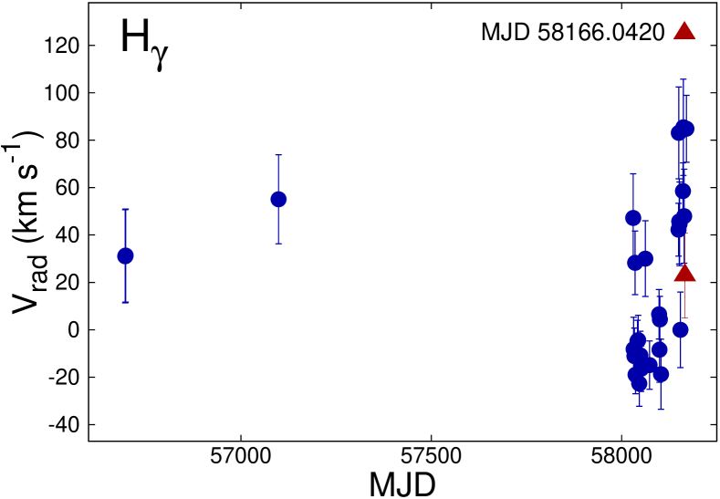
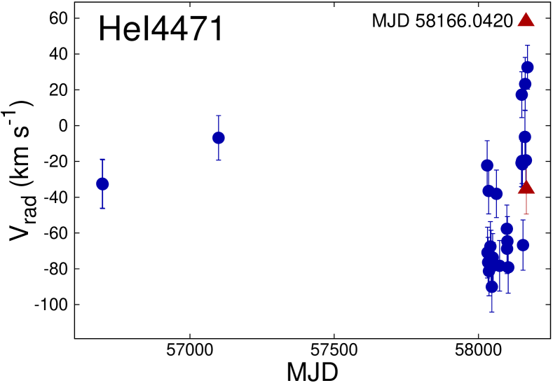
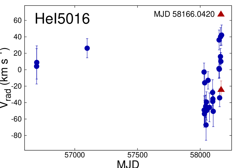
Figure 7: Radial velocities measured for different spectral lines in the observations obtained between 2014 and 2018.

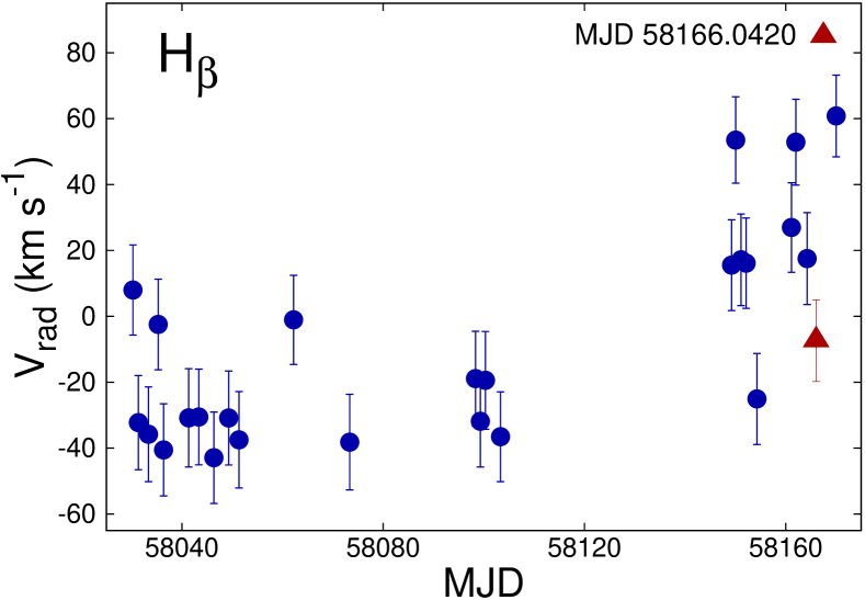
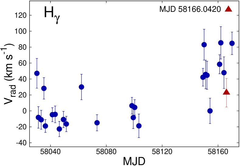
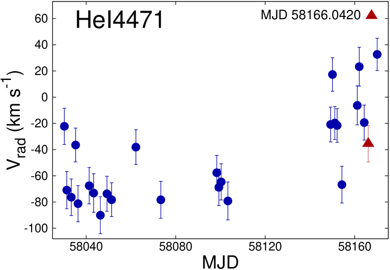
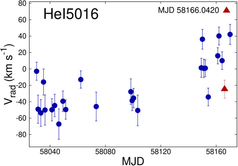
Figure 8: Radial velocities measured for different spectral lines in the observations obtained between 2017 and 2018.

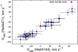
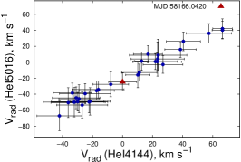
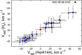
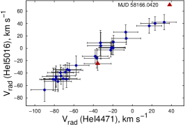
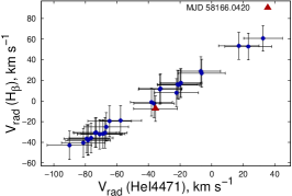
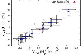
Figure 9: Radial velocity correlations for hydrogen and He i lines.

The radial velocity changes for different lines in all FORS 2 spectra acquired between 2014 and 2018 are presented in Fig. 7 and those measured in our recent spectra between 2017 and 2018 in Fig. 8. While not much can be concluded about the variability of the radial velocities in 2014–2015 due to the rather large measurement uncertainties, the velocity changes in 2017–2018 are more pronounced, indicating an increase by $\sim 100$ km s^-1. Remarkably, we observed at the epoch of the sudden magnetic field increase (indicated by the red triangle) that the radial velocity of all spectral lines dropped by several 10 km s^-1. To better highlight the observed changes in radial velocities, we show in Fig. 9 the radial velocity shift correlations between the lines belonging to different elements.

The observed dispersion of the radial velocity measurements in these figures is probably related to $\beta$ Cephei–like pulsations. The atmospheric parameters presented by Castro et al. (2015) suggest that HD 54879 has already slightly evolved from the ZAMS and is passing through the $\beta$ Cephei instability strip. As mentioned above, Järvinen et al. (2017) were not able to detect significant velocity shifts in high-resolution HARPSpol observations of HD 54879, most likely due to much longer exposure times, of the order of 1–3 h. During the long HARPSpol exposures, any spectral variability is smeared over the pulsation cycle and difficult to detect. In contrast, FORS 2 observations carried out using an 8 m telescope, have a duration of only 10–20 min and are expected to be more strongly affected by the $\beta$ Cephei–like pulsations. According to Telting et al. (2006), at least half of the late O to early B solar-neighbourhood stars that are located in the $\beta$ Cephei instability strip are actually pulsating in radial and/or non-radial modes.

With respect to the remarkable change of the spectral appearance of HD 54879 during the sudden magnetic field increase, it is important to mention that a recent study of the most strongly magnetized O-type star NGC 1624-2 using UV observations with HST/COS revealed similar dramatic variations in the resonance line profiles between rotation phases when looking nearly at the magnetic pole and those when looking nearly at the magnetic equator (see Fig. 1 in David-Uraz et al. 2018). Similar to our observations of HD 54879, these line profiles show at these two rotation phases very different characteristics including the line intensity, line shape and width, and radial velocity. It should however be noted that the variability of the UV resonance lines in massive stars is usually related to the stellar wind or to the magnetosphere, while for HD 54879 we observe line profile changes in the photospheric lines.

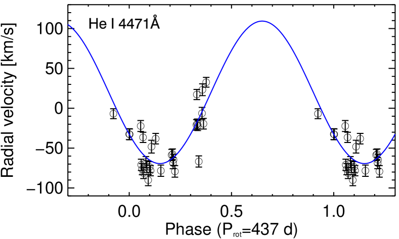
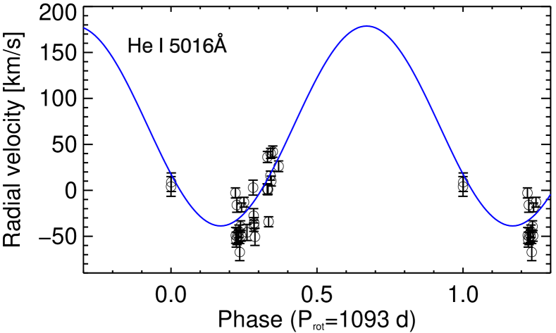
Figure 10: Upper panel: Radial velocities of the He i 4471 line measured in the spectra obtained between 2014 and 2018 are fitted with a period of 437 d. Lower panel: Radial velocities of the He i 5016 line fitted with a period of 1093 d.

It cannot be excluded that the observed changes in radial velocity are caused by an invisible wide companion. Indeed, Castro et al. (2015) compared their radial velocity measurement from one HARPSpol spectrum with other measurements in the literature and concluded that HD 54879 could be a member of a long-period binary system. Our search for periodicity in radial velocities was however rather inconclusive: using radial velocity changes in the line He i 5016 we find an indication of a possible period of 1093 d, while the data for the He i 4471 are better fitted with a period of 437 d. To search for the period, we used a non-linear least-squares fit to multiple harmonics using the Levenberg-Marquardt method (Press et al., 1992). To detect the most probable period, we calculated the frequency spectrum, and for each trial frequency we performed a statistical F-test of the null hypothesis for the absence of periodicity (Seber, 1977). The resulting F-statistics can be thought of as the total sum, including covariances of the ratio of harmonic amplitudes to their standard deviations, i.e. an S/N. The measured radial velocities for both lines fitted with the corresponding periods are presented in Fig. 10. Obviously, due to the poor spectral coverage in the years between 2014 and 2017 and the observed large dispersion of the radial velocity measurements, our results from the period search are only tentative and should be verified by additional spectropolarimetric observations.

4 Discussion

It is the first time that a sudden increase of the magnetic field strength at a rotation phase close to the magnetic equator is observed in a magnetic massive O-type star. As the majority of massive O-type stars rotate rather slowly and rarely are spectroscopically and polarimetrically monitored on several consecutive nights, it is not possible to know whether other magnetic massive stars show sudden increases of their magnetic field strength. On the other hand, the remarkable change of the spectrum of HD 54879 during the magnetic field increase should be easily detected in highly accurate photometric observations.

The nature of magnetic fields in massive stars is still unknown. The presence of magnetic activity is expected since stellar spots, X-ray emission, and flares are observed in OB-type stars (e.g. Groote & Schmitt 2004; Mullan 2009; Smith et al. 1993; Reiners et al. 2000). Such activity indicators can be caused by the presence of arcs and filaments, which however are not discovered yet in massive stars. Within such a scenario, the observed transition to a cooler spectral type and in particular the significant change of the radial velocity of the spectral lines at the time of the sudden magnetic field increase would indicate the presence of a giant temperature spot, which could be related to a large magnetic flux tube that breaks the surface of the photosphere. The dramatic change in radial velocity could then be related to the flow velocity. Similar phenomena are observed in the Sun and solar-like stars, but for smaller scale flux tubes. We can only speculate that the observed cooler spectral type of HD 54879 is probably caused by the increased visibility of the deeper atmospheric layers in the temperature spot and the presence of a non-standard temperature gradient in the upper layers of this massive star due to a large amount of circumstellar absorption related to the large wind confinement radius.

Figure 11: Examples of emission line profiles in the high-resolution HARPSpol spectrum.

Figure 12: Stokes $I$ and Stokes $V$ spectra in the vicinity of a Zeeman feature related to an unidentified emission line with an unknown Landé factor.

Notably, our high-resolution HARPSpol spectra obtained within the framework of the ESO Large Prg. 191.D-0255 indicates that the line formation in the atmosphere of HD 54879 can be quite complex. An anomalous behaviour of weak emission lines in the spectra of the Of?p star NGC 1624-2 with a very strong mean longitudinal magnetic field of the order of 5.35 kG was mentioned in the work of Wade et al. (2012). Opposite to the measurements using absorption lines, measurements using weak O iii emission lines yielded a much lower magnetic field strength of about 2.58 kG. The inspection of the high-resolution HARPSpol spectra of HD 54879 reveals the presence of weak emission lines belonging to C ii, O ii, and Fe iii. Several weak emission lines could, however, not be identified using the Vienna Atomic Line Database. A few examples of identified emission lines are presented in Fig. 11. Due to the relatively low $S/N$, of the order of 200, in the available Stokes $I$ spectra and the weakness of the corresponding Zeeman features, it is currently not possible to conclude on the strength and polarity of the corresponding longitudinal magnetic field. In Fig. 12, we display the strongest Zeeman feature identified in our spectra, which is related to an unidentified emission line with an unknown Landé factor at a wavelength close to 5220.45 Å. If this feature is real, then the inferred longitudinal magnetic field would have positive polarity, which would be inconsistent with the negative polarity measured from the absorption lines ($\langle B_{z}\rangle=-578\pm 21$ G; Järvinen et al. 2017). Obviously, high-resolution spectra obtained at higher S/N are necessary to investigate in detail the emitting regions in HD 54879.

Castro et al. (2015) infer a dipole magnetic field of 2 kG from an observed field strength of $-600$ G. It is, however, not certain that the surface magnetic field of HD 54879 is dipolar. If we assume large magnetic spots, then the dipole field should be substantially smaller and a large fraction of the surface flux will not couple to the stellar wind and form closed magnetic loops instead. The magnetic field strength in sunspots is of the order of kG, but the large-scale surface magnetic field is only of the order of G. The large-scale magnetic field inside the solar convection zone is believed to be much stronger, though, comparable with the magnetic field strength in sunspots. Its configuration is definitely more complicated than a magnetic dipole (e.g. Charbonneau 2014). It seems plausible that any possible dynamo action is located somewhere near the stellar surface and the dynamo-generated magnetic field should be more similar to the magnetic configuration in the solar interior than the configuration at the solar surface. It is therefore possible that the impact of the magnetic field on the stellar wind is weaker than one would expect from a dipole field of 2 kG.

In the following, we will discuss a more sophisticated scenario to explain the HD 54879 observations. First of all, it is possible that current dynamo models slightly underestimate the intensity of dynamo drivers and thus their ability to produce a solar-type dynamo in the convective envelope of HD 54879 (see the discussion of the problem of estimating the intensity of stellar dynamo drivers in Shulyak et al. 2015). Dynamo models usually deal with a more or less typical star of a given spectral type while the physical properties of a particular star can deviate from standard stellar models, e.g. because the star belongs to a binary system. This may explain why the observed phenomenon is not common for all O-type stars. Moss, Piskunov & Sokoloff (2002) studied an $\alpha^{2}$-dynamo with a non-axisymmetric distribution of the $\alpha$-effect caused by tidal forces in a close binary system. This type of dynamo produces large surface spots through the large-scale field, i.e. the radial component of the mean field is strongly concentrated at certain longitudes on the stellar surface. Adding differential rotation then causes the magnetic field to oscillate, but without the migration pattern shown by $\alpha^{2}$-dynamos with axisymmetric $\alpha$-effect. While this scenario creates surface spots without requiring flux tubes being brought to the surface by buyoancy, the assumption of a strong deviation from axisymmetry in the $\alpha$-effect seems far-fetched in the context of HD 54879.

Even if the solar-type dynamo in HD 54879 remains subcritical and dynamo drivers such as differential rotation and mirror asymmetric convection produce a more complicated magnetic field than in the solar case, the dynamo-generated field configuration can be rather simple, for example of quadrupolar symmetry (this option is discussed for stellar dynamos by e.g. Moss, Saar & Sokoloff 2008). Stellar winds associated with a quadrupole magnetic field have not attracted much attention so far and at least some research is required here to rule them out.

In principle, dynamo drivers in HD 54879 may be insufficiently intensive to produce an oscillating magnetic field from a weak seed field, yet sufficient to maintain an already existing magnetic field. Such hysteresis dynamos are discussed by Karak, Kitchatinov & Brandenburg (2015). Fossil magnetic fields as presumed in O-type stars by Moss (2003) may provide the initial magnetic field required for hysteresis effects. Such a scenario has been discussed by Singh, Rogachevskii & Brandenburg (2017) in a different context. Small-scale dynamo action which provides substantial magnetic flux and is modulated by a subcritical oscillating solar-type magnetic configuration also seems to be an option that deserves investigation (cf. Yushkov, Lukin & Sokoloff 2018).

In the following subsections we consider the impact of a dipole field on the stellar wind, the available X-ray observations, and discuss other probable scenarios in an attempt to interpret our observations.

4.1 Magnetic field impact on the stellar wind

The impact of a dipole magnetic field rooted in the star on the stellar wind can be characterised by the confinement parameter

$$\eta_{*}=\frac{B^{2}_{\rm eq}R^{2}_{*}}{\dot{M}v_{\infty}},$$ (1)

(ud-Doula & Owocki, 2002) where $B_{\rm eq}$ is the magnetic field strength at the equator, $R_{*}$ the stellar radius, $\dot{M}$ the mass loss rate, and $v_{\infty}$ the terminal wind speed. ud-Doula, Owocki & Townsend (2008) found a strong reduction of the mass loss rate for the case of strong confinement, when magnetic field lines originating close to the magnetic equator remain closed and the outflowing gas will thus be trapped at these latitudes. In the equatorial plane magnetic field lines will remain closed up to the confinement radius

$$R_{c}\approx R_{*}+0.7(R_{A}-R_{*}),$$ (2)

where $R_{A}$ is the Alfvén radius

$$R_{A}\approx\left(0.3+0.7\eta^{1/4}_{*}\right)R_{*}.$$ (3)

Magnetic field lines that originate at angles larger than $\theta_{c}$ given by

$$\sin\theta_{c}=\sqrt{R_{*}/R_{c}}$$ (4)

from the magnetic poles remain closed. Gas can only escape through caps around the magnetic poles where open field lines originate. The mass loss rate is reduced by the factor

$$\frac{\dot{M_{B}}}{\dot{M_{B=0}}}\approx 1-\sqrt{1-R_{*}/R_{c}}$$ (5)

relative to the case where the magnetic field is absent.

Table 2: Values of the confinement parameter and the reduction of the mass loss rate

$B_{*}$	$\eta_{*}$	$R_{c}/R_{\odot}$	$\dot{M}/\dot{M_{0}}$
(G)
100	42	1.757	0.3436
300	380	2.674	0.2088
800	$2.7\times 10^{3}$	4.042	0.1325
2000	$1.7\times 10^{4}$	6.105	0.08556

Table 3: Stellar parameters adopted for the numerical simulations.

$T_{*}$	(${\rm kK}$)	30.5
$\log L$	($L_{\odot}$)	4.42
$R_{*}$	($R_{\odot}$)	6.1
$M_{*}$	($M_{\odot}$)	14
$\log\dot{M_{0}}$	($M_{\odot}\,{\rm yr}^{-}1)$	$-9$
$\log\dot{M_{B}}$	($M_{\odot}\,{\rm yr}^{-1}$)	$-10.2$
$v_{\infty}$	(km s-1)	1700

Table 2 lists the confinement parameter, confinement radius, and mass loss rate for various values of the magnetic field strength. The effect of stronger fields is a larger extent of the magnetically-dominated region, as indicated by the confinement radius and a further reduction of the mass loss rate. The stellar parameters have been adopted from Shenar et al. (2017) and are listed in Table 3.

To illustrate this reduction in the mass loss rate and the distribution of the trapped gas, we have carried out a series of numerical simulations using the Nirvana MHD code (Ziegler, 2011). The setup is similar to that described in Küker (2017). The simulation box is a spherical shell with the stellar surface as the inner boundary. The outer boundary is typically at a radius of 10 stellar radii. The magnetic field is kept fixed on the inner boundary and can evolve elsewhere. We set a fixed mass density on the lower boundary and let the radial velocity float. At the outer boundary, the Nirvana code’s built-in outflow conditions are used. Likewise built-in boundary conditions are used on the symmetry axis.

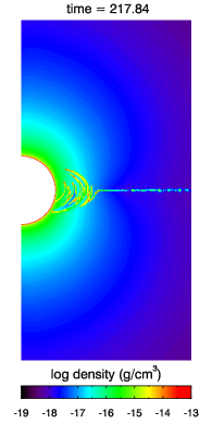
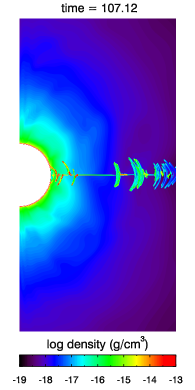
Figure 13: Snapshots from simulations of a line-driven wind and a dipole magnetic field rooted in the star. The polar field strength is 100 G (left) and 300 G (right). Colours indicate mass density.

As simulations for polar field strengths of 800 G and 2 kG proved to be very time consuming, we studied the first two cases listed in Table 2, namely 100 G and 300 G. Fig. 13 shows snapshots of the mass density. As indicated by the values of 42 and 380 for the confinement parameter, the magnetic field has a profound impact on the gas flow. The 100 G case shows a fully-developed magnetosphere while in the 300 G case the magnetosphere is still forming. The circular cutout at the left margins of the plots marks the star. The left margin is the dipole axis of the magnetic field. Stellar rotation was not included, hence the dipole axis of the magnetic field defines the symmetry. Outside the confinement radius $R_{c}$, gas still concentrates in elongated structures along the magnetic field lines, but is ejected away from the star in episodic outbursts.

While for very weak magnetic fields – a small value of the confinement parameter – the mass loss is steady, our simulations show episodic outbreaks of gas previously trapped near the magnetic equator. These mass ejections are typical for the case of strong confinement, which is fulfilled even for the weakest field of 100 G considered here. During the outbursts, which last about a day, clumps of gas move away from the star in the equatorial plane of the magnetic field at high speed. The contribution of these outbursts to the total mass loss rate reaches values of the same order as that of the steady wind component, i.e. the total mass loss rate during the outburst can be twice as high as during the quiet phase in between. This is in contrast to cases of weak confinement, $\eta_{*}<1$, where a steady disk forms and the mass loss rate shows little variation with time. Obviously, the interaction of the stellar magnetic field with the wind does not explain the drop in effective temperature and in radial velocity observed during the episode of a strong surface magnetic field.

4.2 X-ray spectral analysis

As our MHD model is isothermal, we cannot make direct predictions regarding the X-ray emission that is expected from the material trapped inside the confinement radius. It is obvious, however, that X-ray radiation originates from areas near the equatorial plane of the magnetic field. Gagne et al. (2005) carried out numerical simulations for the star $\theta^{1}$ Ori C in which the energy equation was included. With a cooling function adopted from MacDonald & Bailey (1981), they found that shock heating would bring the compressed material to temperatures of up to 30 MK. The emission measure calculated from the distributions of mass density and temperature matched those observed by the High Energy Transmission Grating spectrometer (HEGT) onboard the Chandra space observatory.

A single observation in the X-ray region of HD 54879 was acquired by XMM-Newton with an exposure time of about 40 ks (ObsId = ”0780180101”) on 2016 May 1. A previous analysis of these observations was published by Shenar et al. (2017) who concluded that the X-ray spectrum can be fitted with a thermal model accounting for either two or three components, and implies a higher-than-average X-ray luminosity ($\log L_{\text{X}}/L_{\text{bol}}=-6.0$). Assuming the three-component model, their result indicates an X-ray temperature reaching values of up to $T_{\text{X}}\approx 20\,$MK.

Table 4: X-ray spectral parameters derived from the XMM-Newton observations of HD 54879 assuming different plasma models. The first column lists the applied models, followed by the hydrogen column density, the plasma temperatures, the photon index $\Gamma$, and the element abundances. The indicator of the approximation accuracy $\chi^{2}$ and the degrees of freedom are presented in the last column. The three models with missing entries did not produce any reasonable fitting parameters.

Model	$N_{H}$	$kT_{1}$	$kT_{2}$	$kT_{3}$	$\Gamma$	Abundance	$\chi^{2}$
	($10^{22}cm^{-2})$	(keV)	(keV)	(keV)	(rel. un.)	(rel. un.)	(d.o.f)
PN
WABS$\cdot$APEC	$0.13^{+0.02}_{-0.02}$	$0.76^{+0.03}_{-0.03}$	-	-	-	$0.20^{+0.05}_{-0.04}$	1.61 (107)
WABS$\cdot$(APEC+APEC)	$0.34^{+0.12}_{-0.09}$	$0.74^{+0.04}_{-0.24}$	$0.18^{-0.03}_{+0.03}$	-	-	$0.58^{+1.72}_{-0.24}$	1.23 (105)
WABS$\cdot$(APEC+APEC+APEC)	$0.50^{+0.10}_{-0.19}$	$0.11^{+0.07}_{-0.05}$	$0.28^{+0.80}_{-0.06}$	$0.77^{+0.09}_{-0.07}$	-	$\leq$0.63	1.17 (103)
WABS$\cdot$(APEC+PL)	-	-	-	-	-	-	-
WABS$\cdot$(APEC+APEC+PL)	$0.30^{+0.03}_{-0.17}$	$0.35^{+0.05}_{-0.04}$	$0.86^{+0.29}_{-0.05}$	-	$3.98^{+0.37}_{-0.37}$	$1.90^{+3.10}_{-0.50}$	1.47 (103)
WABS$\cdot$MEKAL	$0.17^{+0.03}_{-0.02}$	$0.61^{+0.03}_{-0.03}$	-	-	-	$0.18^{+0.05}_{-0.04}$	1.46 (107)
WABS$\cdot$(MEKAL+MEKAL)	$0.33^{+0.09}_{-0.08}$	$0.18^{+0.03}_{-0.03}$	$0.60^{+0.04}_{-0.04}$	-	-	$0.43^{+0.57}_{-0.16}$	1.23 (105)
MOS1+MOS2
WABS$\cdot$APEC	$0.14^{+0.03}_{-0.03}$	$0.74^{+0.04}_{-0.04}$	-	-	-	$0.14^{+0.04}_{-0.03}$	1.07 (118)
WABS$\cdot$(APEC+APEC)	$0.26^{+0.11}_{-0.09}$	$0.75^{+0.08}_{-0.05}$	$0.21^{+0.11}_{0.05}$	-	-	$0.18^{+0.12}_{-0.06}$	1.02 (116)
WABS$\cdot$(APEC+APEC+APEC)	-	-	-	-	-	-	-
WABS$\cdot$(APEC+PL)	$0.64^{+0.06}_{-0.19}$	$0.24^{+0.11}_{-0.02}$	-	-	$3.70^{+2.02}_{-0.55}$	$2.02^{+3.08}_{-1.66}$	1.30 (116)
WABS$\cdot$(APEC+APEC+PL)	-	-	-	-	-	-	-
WABS$\cdot$MEKAL	$0.18^{+0.03}_{-0.03}$	$0.60^{+0.03}_{-0.03}$	-	-	-	$0.12^{+0.03}_{-0.03}$	1.05 (118)
WABS$\cdot$(MEKAL+MEKAL)	$0.27^{+0.11}_{-0.08}$	$0.20^{+0.10}_{-0.05}$	$0.60^{+0.05}_{-0.04}$	-	-	$0.17^{+0.10}_{-0.05}$	1.02 (116)

Figure 14: Left panel: The MOS spectrum (crosses) together with the model WABS$\cdot$MEKAL (solid line). Right panel: The PN spectrum (crosses) together with the model WABS$\cdot$MEKAL (solid line). The bottom panels show the residuals of the fit.

We re-analysed the available XMM-Newton data using the SAS 17.0 software, following the recommendations of the SAS team. We modeled the band 0.2-8 keV of the EPIC-PN spectrum and EPIC-MOS1+EPIC-MOS2 spectra using the xspec 11.0 package. The spectra were fitted by a composition of one or two temperature thermal plasma models (APEC or MEKAL) and a nonthermal power law (PL) model, which describes synchrotron emission. All model compositions were multiplied by the photoelectric absorption model WABS for taking into account interstellar absorption. The best fits are listed in Table 4 and examples of the spectral modeling are shown in Fig. 14.

Our results presented in Table 4 indicate that the X-ray spectrum of HD 54879 can be described by thermal plasma models, in agreement with the results of Shenar et al. (2017). However, our fits are more accurate. We note that the spectrum can also be accurately fitted by the sum of APEC and PL models. A PL model would imply that hard X-rays arise from relativistic electrons generated through an acceleration mechanism involving strong shocks. In this model, we would expect a value close to 1.5 for the photon index. However, since we found much higher values for the photon index, this scenario is less likely.

The RGS1$+$RGS2 spectrum of HD 54879 was not considered in the study of Shenar et al. (2017). In the spectral band of 6-38 Å we identified several lines using an approximation of the line profiles by a sum of Gauss or Gauss-like functions. This method is described in Section 3 of Ryspaeva & Kholtygin (2018). The identified lines were used to calculate the spectral hardness as a ratio of fluxes in lines of adjacent ions. To calculate the hardness ratios, we used the following lines of ions that are widespread in the spectra of O-stars: Fe XXII/Fe XXI, Fe XXI/Fe XX, Fe XX/Fe XIX, Fe XIX/Fe XVIII, Fe XVIII/Fe XVII, Fe XVII/Fe XVI, Ca XV/Ca XIV, Ca XIV/Ca XIII, Ca XIII/Ca XII, Ca XII/Ca XI, Ar XV/Ar XIV, and Ar XIV/Ar XIII. The resulting hardness ratios were found in the range $9.8\times 10^{-2}$ to $1.46\times 10^{1}$ relative units and are comparable to those of other O-type stars presented in Figs. 5 and 6 in the work of Ryspaeva & Kholtygin (2018). To conclude, the results of our analysis of the XMM-Newton observations are not significantly different compared to the analysis of other O-type stars.

4.3 Other scenarios

For the rapid changes of the magnetic field strength the appearance and decay of magnetic spots seems more likely than a variation of a dipole field. Previous spectroscopic studies of massive stars revealed a variety of spectral variability: discrete absorption components (DACs) in UV P-Cygni profiles, optical line profile variability, radial velocity modulations, etc. Spectroscopic time series observations frequently show different absorption features propagating with different accelerations at the same time. Such features are thought to be signatures of corotating interaction regions (CIRs) in the winds (Mullan, 1984). While DACs are ubiquitous among O-type stars, only for a number of massive stars the current analysis of dynamic UV spectra securely establishes that the variability has a photospheric origin and does not originate near the stellar surface (e.g. Massa & Prinja 2015). For stars showing CIRs, it has been known for a long time that the absorption features seen in dynamic spectra must be huge in order to remain in the line of sight for days. This means that the linear size of the region responsible for the excess absorption must be at least 15–20 per cent of the stellar diameter and, in some cases, considerably larger. According to Cantiello & Braithwaite (2011a), convection zones could also be responsible for generating sub-surface magnetic fields via dynamo action and thereby can account for localized corotating magnetic structures. They proposed a dynamo in the iron convection zones (FeCZ) of OB stars as a mechanism for the generation of surface magnetic fields brought to the surface by buoyancy. While the gas density in the FeCZ is small, the convection velocities are large enough to sustain magnetic fields of the observed strength. The effect of convection zones in massive stars is expected to increase with increasing luminosity and lower effective temperature (Cantiello et al., 2009). The nature of the dynamo remains unclear, though.

Cantiello et al. (2011b) carried out 3D MHD simulations that showed the generation of a magnetic field, but rotation and shear were required to produce a large-scale magnetic field. Bipolar groups of sunspots are believed to be created by the buoyant rise of toroidal flux tubes, which are generated by rotational shear. The slow rotation, however, makes this mechanism unlikely for HD 54879. While a different spot formation mechanism is possible, it is doubtful that a dynamo in the FeCZ of the star could generate a large-scale magnetic field. The situation could be different in the convective core, which might rotate much faster than the envelope. Rapid rotation would not only favour the generation of a large-scale magnetic field in the core, the shear between core and envelope would then generate strong toroidal fields, which could rise to the surface and form magnetic spots there.

One can speculate that a short increase of the longitudinal magnetic field as observed in HD 54879 may support the scenario of sudden magnetic field ejections into the stellar wind that is used to explain the bright X-ray flares in supergiant fast X-ray transients. Shakura et al. (2014) proposed a mechanism to explain in these binaries the observed sporadic X-ray flares. It is based on an instability of the quasi-spherical shell around the magnetosphere of a slowly rotating neutron star (NS). The authors suggest that the instability can be triggered by the sudden increase in the mass accretion rate through the magnetosphere due to reconnection of the large-scale magnetic field sporadically carried by the stellar wind of the optical OB-companion. The bright flares due to the proposed mechanism can occur on top of a smooth variation of mass accretion rate due to, for example, orbital motion of the NS in a binary system.

To summarize, our results presenting strong magnetic and spectral variability detected during a very short time interval clearly show that careful spectropolarimetric monitoring even of stars with very long rotation periods is necessary to better understand the processes taking place in massive stars. Additional X-ray observations are in particular important to fully characterize the wind material confined by the magnetic field of HD 54879. While the discussed scenarios may have some potential in clarifying the sudden increase of the longitudinal magnetic field, they are currently unable to fully explain the observed phenomena. The role of an invisible companion is also not clear, as there is no working theoretical prediction on how an invisible companion could affect the magnetic field strength and the spectral appearance of a massive O-type star just for a very short time interval.

References

- Appenzeller et al. (1998) Appenzeller I., et al., 1998, The ESO Messenger, 94, 1
- Borra et al. (1982) Borra E. F., Landstreet J. D., Mestel L., 1982, ARA&A, 20, 191
- Brun, Browning & Toomre (2005) Brun A. S., Browning M. K., Toomre J., 2005, ApJ, 629, 461
- Cantiello et al. (2009) Cantiello M., et al., 2009, A&A, 499, 279