Valence bond fluctuations in the Kitaev spin model

Abstract

We introduce valence bond fluctuations, or bipartite fluctuations associated to bond-bond correlation functions, to characterize quantum spin liquids and the entanglement properties of them. Using analytical and numerical approaches, we find an identical scaling law between valence bond fluctuations and entanglement entropy in the two-dimensional Kitaev spin model and in one-dimensional chain analogues. We also show how these valence bond fluctuations can locate, via the linear scaling prefactor, the quantum phase transitions between the three gapped and the gapless Majorana semi-metal phases in the honeycomb model. We then study the effect of a uniform magnetic field along the $[111]$ direction opening a gap in the intermediate phase which becomes topological. We still obtain a robust signal to characterize the transitions towards the three gapped phases. The area law behavior of such bipartite fluctuations in two dimensions is also distinguishable from the one in the Néel magnetic state that follows a volume square growth.

I Introduction

The quest of quantum spin liquids in the Mott regime [1, 2, 3, 4, 5, 6] has been a great challenge these last decades in relation with the discovery of quantum materials [7, 8, 9, 10, 11, 12, 13, 14, 15]. Quantum spin liquids show interesting topological and entanglement properties [16, 17, 18, 19] which can be used for applications in quantum information [20]. The Kitaev spin model on the honeycomb lattice [21] represents an important class of models, since it can be solved exactly in a Majorana fermion representation and demonstrates the significance of $\mathbb{Z}_{2}$ gauge fields on the low-energy properties. The model shows three gapped spin liquid phases carrying Abelian anyon excitations and an intermediate gapless phase which can be identified as a semi-metal of Majorana fermions. Applying a magnetic field along the three spatial directions [21], referring to a field in the $[111]$ direction, induces a gap in the intermediate phase, then producing a topological $\mathbb{Z}_{2}$ phase supporting non-Abelian anyonic excitations [22] and closely related to a $p_{x}+ip_{y}$ superconductor [23] with chiral edge modes. It is important to emphasize that static spin-spin correlation functions are exactly zero beyond nearest neighbors in this model [24]. Theoretical efforts have been performed to compute dynamical correlation functions [25, 26, 27, 28, 29] as well as the entanglement entropy [30, 29]. By bipartitioning a system spatially, the entanglement entropy measures how entangled the two subsystems are [31]. Related to these theoretical developments, quasi-two-dimensional quantum materials have been synthesized [32, 33, 34], with recent measurements from neutron [35] and Raman [36] scatterings, nuclear magnetic resonance [37] and thermal transport [38, 39, 40]. One and two-dimensional Kitaev spin liquids, could also be engineered in ultra-cold atoms [41] and quantum circuits  [42, 43].

In this Article, we propose valence bond fluctuations as a probe of entanglement properties in the ground state of the Kitaev spin model.

A valence bond (VB) [3] here corresponds to the spin-spin pairing between two nearest neighbor electrons. Our first insight comes from the system of SU(2)-symmetric quantum spins with resonating valence bonds (RVB) where we find the bond fluctuations can be related to valence bond entropy of Einstein-Podolsky-Rosen (EPR) pairs or Bell pairs [44]. Extending to the Kitaev spin liquids, in the three gapped phases, the valence bonds between nearest neighbors form a crystalline or dimer order [21]. Approaching the transition(s) to the gapless intermediate phase, these bonds now resonate giving rise to gapless critical fluctuations, which in principle encode information on quantum phase transitions and entanglement properties. Our calculations indeed reveal an identical scaling between valence bond fluctuations and entanglement entropy in one-dimensional chain and two-dimensional honeycomb lattice, and we check our mathematical findings with numerical calculations, e.g. through the Density Matrix Renormalization Group (DMRG). In one dimension, the gapless phase is reduced to a quantum critical point [45], which then develops into a plane for ladder systems [46]. In two dimensions, in the absence of a magnetic field, the long-range valence bond correlations in space [47] share a similar scaling as the dynamical spin structure factor [25]. We include also the effects of a uniform magnetic field in the perturbative regime, and discuss relevant consequences from the excitations of flux pairs [27] and from the formation of U(1) gapless spin liquids once three Ising couplings become anti-ferromagnetic (AFM) [48]. In the end, to make a closer link with quantum materials, we give a comparison of valence bond fluctuations in the Néel state favored by strong AFM Heisenberg exchanges.

II Review of Fluctuations as An Entanglement Probe

First, we begin with a brief review on the relation between bipartite fluctuations and entanglement entropy in many-body Hamiltonians characterized by different symmetries [49, 50, 51, 52]. In Sec. II.1, we define the general fluctuations on a bipartite lattice, which from the information theory, provide a lower bound for the mutual information related to entropy. We then remind in Sec. II.2, an exact expression for the entropy as a series expansion of even cumulants (with particle number or spin fluctuations the leading order) for the U(1) charge conserved systems [49] and an inequality between the two quantities emerging among the SU(2) quantum spins described by resonating valence bonds.

Generalizing these works to Kitaev spin liquids coupled to a gapped $\mathbb{Z}_{2}$ gauge field represents our central motivation in this work. The difficulty lies in finding the right observable encoding the long-range correlation of matter Majorana fermions in the gapless phase, hence the entanglement properties. Fortunately, by analogy to the RVB states in the three gapped phases, in Sec. II.3 we verify that the valence bond fluctuations represent non-vanishing lower bound for the entropy.

II.1 Generalities

We decompose a generic quantum system into two parts $A\cup B$. For the subsystem $A$, the entanglement is measured by the von Neumann entropy [31]

$$\mathcal{S}_{A}=-\text{Tr}{\rho}_{A}\ln{\rho}_{A},$$ (2.1)

where ${\rho}_{A}=\text{Tr}_{B}\rho$ represents the reduced density matrix of sub-system $A$. Once given two density matrices $\rho$ and $\rho^{\prime}$, the distance between two states can be probed by the relative entropy

$$\mathcal{S}(\rho,\rho^{\prime})=\text{Tr}\left[\rho(\log\rho-\log\rho^{\prime})\right],$$ (2.2)

with a norm bound [53]

$$\mathcal{S}(\rho,\rho^{\prime})\geq\frac{1}{2}\left||\rho-\rho^{\prime}|\right|^{2}.$$ (2.3)

Here the norm stands for $\left||\rho|\right|=\text{Tr}\sqrt{\rho^{\dagger}\rho}$ and we have assumed that $\hbox{Tr}\rho=\hbox{Tr}\rho^{\prime}=1$. Making an analogy with vectors, one may also write $S(\rho,\rho^{\prime})=S(\rho\parallel\rho^{\prime})$. For instance, for diagonal (density) matrices, each eigenvalue may refer to a coordinate along one direction. On the other hand, to evaluate the fluctuations, we introduce two measurements

$$\mathcal{F}_{A}=\left<\left(\sum_{i\in A}Q_{i}\right)^{2}\right>_{c},$$ (2.4)

$$\mathcal{F}_{AB}=\left|\sum_{i\in A}\sum_{j\in B}\left<Q_{i}Q_{j}\right>_{c}\right|.$$ (2.5)

Here, $Q$ is a chosen operator for targeted systems: charge, particle number, one spin or two spins on a valence bond and $\left<Q_{i}Q_{j}\right>_{c}=\langle Q_{i}Q_{j}\rangle-\langle Q_{i}\rangle\langle Q_{j}\rangle$ denotes the reduced correlation function. It is easy to notice while $\mathcal{F}_{A}$ measures the fluctuations in subsystem $A$, $\mathcal{F}_{AB}$ covers the correlations between $A$ and $B$. There is an equality between the two quantities:

$$\mathcal{F}_{AB}=\frac{1}{2}\left|\mathcal{F}_{A}+\mathcal{F}_{B}-\mathcal{F}_{A\cup B}\right|.$$ (2.6)

An important finding so far established is to relate $\mathcal{F}_{AB}$ with $\mathcal{S}_{A}$ by mutual information [54]

$$I(A,B)=\mathcal{S}_{A}+\mathcal{S}_{B}-\mathcal{S}_{A\cup B}.$$ (2.7)

From the definition of relative entropy (2.2), the mutual information has an alternative expression

$$I(A,B)=\mathcal{S}(\rho_{A\cup B},\rho_{A}\otimes\rho_{B}).$$ (2.8)

Choosing any operator of the matrix form $Q=Q_{A}\otimes Q_{B}$ with $Q_{A}$ the bounded operator in region $A$ and applying the Schwarz inequality $\left||\rho|\right|\geq\text{Tr}(\rho Q)/\left||Q|\right|$ to the norm bound (2.3), one obtains [55]

$$I(A,B)\geq\frac{\left(\langle Q_{A}Q_{B}\rangle-\langle Q_{A}\rangle\langle Q_{B}\rangle\right)^{2}}{2\left||Q_{A}|\right|^{2}\left||Q_{B}|\right|^{2}}.$$ (2.9)

The numerator recovers $\mathcal{F}_{AB}$. Correspondingly, for $\mathcal{F}_{AB}\neq 0$, we arrive at

$$\frac{I(A,B)}{\mathcal{F}_{AB}}\geq\text{cst}.$$ (2.10)

Although the lower bound between the bipartite fluctuations and the mutual information is universal, it remains ambiguous what is the form of operator $Q$ one should choose for a given many-body system such that the fluctuations measured are non-vanishing. A second inquiry would be: under which circumstances we could reach the equality of (2.10) such that the fluctuations share the same scaling as the original entropy.

II.2 Exact relations and inequalities

In this subsection, we give two known examples where one can relate entanglement entropy directly to charge or spin fluctuations. We further show in Sec. II.2.2, for the SU(2)-symmetric RVB state, that the bond correlator is also a good option for operator $Q$.

II.2.1 Noninteracting fermions with conserved U(1) charge

Let us consider a system of non-interacting fermions with conserved total charge, or more precisely total number of particles: $\hat{N}_{\text{tot}}|\psi\rangle=N_{\text{tot}}|\psi\rangle$. At zero temperature, the ground state $|\psi\rangle$ of the total system becomes pure. Basic properties of the entanglement entropy then follow

• symmetric: $\mathcal{S}_{A}=\mathcal{S}_{B}$;

• subadditive: $\mathcal{S}_{A}+\mathcal{S}_{B}\geq\mathcal{S}_{A\cup B}=0$.

Without any calculation, one can already see the similarities between charge fluctuations and the entropy. If we take $\hat{Q}_{A}=\hat{N}_{A}$ in $\mathcal{F}_{A}$ (2.4), where $\hat{N}_{A}$ represents the number of particles in sub-region $A$, as a result of total charge conservation $\hat{N}_{A}-N_{A}=-(\hat{N}_{B}-N_{B})$, the fluctuations also inherit the symmetric and sub-additive characteristics

$$\mathcal{F}_{A}=\mathcal{F}_{B},\qquad\mathcal{F}_{A}+\mathcal{F}_{B}=2\mathcal{F}_{A}\geq 0.$$ (2.11)

In fact, one can relate the two quantities more rigorously by the cumulant expansion of entropy [49]

$$\mathcal{S}_{A}=\lim_{K\to\infty}\sum_{n=1}^{\lfloor(K+1)/2\rfloor}\alpha_{2n}(K)C_{2n}.$$ (2.12)

Here, the coefficients are all positive and related to the unsigned Stirling number of the first kind: $\alpha_{n}(K)=2\sum_{k=n-1}^{K}S_{1}(k,n-1)/(k!k)$. The cumulants $C_{n}$ are given by the generating function $\chi(\lambda)=\langle e^{i\lambda\hat{N}_{A}}\rangle$ according to

$$C_{n}=\left.(-i\partial_{\lambda})^{n}\ln\chi(\lambda)\right|_{\lambda=0}.$$ (2.13)

By definition, one verifies $\mathcal{F}_{A}=C_{2}$. For a Gaussian process, one can truncate the serie with $K=1$, but for non-Gaussian models one needs to check carefully the convergence of the series with the appropriate number of cumulants [49]. As a comparison, if we consider a Bell pair or an EPR pair, then this generally requires around 10 cumulants to reproduce the $\ln 2$ entropy. Although the equivalence of entropy and a complete set of even cumulants $(\ref{eq:sc})$ is unique to the systems with a mapping to non-interacting fermions, the general relation between entropy and fluctuations (2.14) can be further extended to the interacting one-dimensional (1D) critical systems that conserve total charge, and can be described by a Gaussian model through conformal field theory (CFT) or bosonization. In those cases, $\mathcal{S}_{A}$ can also be truncated by a $K=1$ upper-bound. Thus one gets

$$\frac{\mathcal{S}_{A}}{\mathcal{F}_{A}}\simeq\text{cst}.$$ (2.14)

The constant proves to encode rich information, for instance [49]

$$\text{cst}\cdot\frac{3}{\pi^{2}}=\begin{cases}K,&\text{Luttinger liquids};\\ c/g,&\text{U(1) CFTs},\end{cases}$$ (2.15)

where similarly to Refs. [49, 56], we also introduce the letter $K$ for the Luttinger parameter and $c$ represents the central charge in conformal field theory (CFT). Parameter $g=\pi v\kappa$ consists of the velocity $v$ and compressibility $\kappa=\partial n/\partial\mu$.

II.2.2 SU(2) quantum spins with EPR pairs

Intuitively, one may wonder what will happen when the system breaks U(1) charge conservation and when the system becomes higher dimensional, such as two-dimensional. Next, we give an example of the SU(2)-symmetric valence bond state [49]. Indeed, a direct correspondence in terms of inequality similar to relation $(\ref{eq:sf})$, subsists if we replace $\mathcal{F}_{A}$ with $\mathcal{F}_{AB}$, by analogy to mutual information (2.10). Furthermore, we would like to extend the result of Ref. [49] and show how the two-spin fluctuations and valence bond fluctuations capture different features of the entanglement entropy. Here, by “two-spin fluctuations”, we refer to fluctuations associated to spin-spin correlation functions. From Eq. (2.5), two-spin (TS) fluctuations and valence bond fluctuations between two subregions read:

$$\mathcal{F}^{\text{TS}} = \mathcal{F}_{AB}(Q_{i,\alpha}=\sigma^{z}_{i,\alpha}),$$

$$\mathcal{F}^{\text{VB}} = \mathcal{F}_{AB}(Q_{i}=\sigma^{z}_{i,1}\sigma^{z}_{i,2}).$$ (2.16)

In this work, our aim is to show that the valence bond fluctuations are essential since they provide relevant information both for SU(2) and $\mathbb{Z}_{2}$ quantum spin liquids.

We consider the two-dimensional Heisenberg antiferromagnetic (HAF) model where arise two competing phases: a Néel state and a gapped VB state. In either configuration, the valence-bond entropy has proven to exhibit distinct behaviors [44]:

$$\mathcal{S}^{\text{VB}}_{\text{2D HAF}}\sim\begin{cases}ax\ln x+bx&(\text{N\'{e}el})\\ b^{\prime}x&(\text{VB})\end{cases}.$$ (2.17)

Here $x$ denotes the length of the boundary between two subsystems. This measure can also accurately detect quantum phase transitions between Néel and RVB spin phases in quasi-one dimensional ladder systems [57]. For the moment, we focus on the fluctuations of the gapped VB state and will address the comparison with a Néel state later in Sec. V.2.

Suppose our system comprises $N$ sites on even and odd sublattices. Dimer coverings between different sublattices sharing the form

$$|\frown\ \rangle_{\overline{(i,1)(j,2)}}=\frac{1}{\sqrt{2}}(|\uparrow_{i,1}\rangle|\downarrow_{j,2}\rangle-|\downarrow_{i,1}\rangle|\uparrow_{j,2}\rangle),$$ (2.18)

minimize the energy from the antiferromagnetic Heisenberg interactions. The subscript $(i,\alpha)$ describes the site on $i$-th unit cell of the $\{\alpha=1,2\}$ sublattice. A singlet state $|\Phi_{0}\rangle$ can then be represented as a complex superposition of all possible dimer or pairing configurations

$$|\Phi_{0}\rangle=\sum_{p}\lambda_{p}|\varphi_{p}\rangle,$$

$$|\varphi_{p}\rangle=\prod_{\overline{(i,1)(j,2)}\in p}|\frown\ \rangle_{\overline{(i,1)(j,2)}}.$$ (2.19)

For a given global pairing distribution $p$, the product state goes over all local internal dimers $\overline{(i,1)(j,2)}$.

The corresponding VB entanglement entropy (2.17) is defined as [44]

$$\mathcal{S}^{\text{VB}}(\Phi_{0})=\frac{\sum_{p}\lambda_{p}\mathcal{S}^{\text{VB}}(\varphi_{p})}{\sum_{p}\lambda_{p}}.$$ (2.20)

Formally, acting on the singlet state $|\Phi_{0}\rangle$, the fluctuations and the VB entropy can be obtained from the decomposition (2.19)

$$\mathcal{F}^{\text{TS/VB}}(\Phi_{0}) =\sum_{p}\sum_{p^{\prime}}\lambda_{p}^{*}\lambda_{p^{\prime}}\mathcal{F}^{\text{TS/VB}}(\varphi_{p},\varphi_{p^{\prime}}),$$

$$\mathcal{S}^{\text{VB}}(\Phi_{0}) =(\ln 2)\cdot\frac{\sum_{p}\lambda_{p}\mathcal{F}^{\text{TS}}(\varphi_{p},\varphi_{p})}{\sum_{p}\lambda_{p}}.$$ (2.21)

Eq. (2.21) indicates in general there is no simple correspondence between $\mathcal{F}^{\text{TS/VB}}$ and $\mathcal{S}^{\text{VB}}$. Yet, we may try to simplify (2.21) as

$$\mathcal{F}^{\text{TS/VB}}(\Phi_{0}):=\sum_{p}|\lambda_{p}|^{2}\mathcal{F}^{\text{TS/VB}}(\varphi_{p},\varphi_{p}).$$ (2.22)

For $\mathcal{F}^{\text{TS}}$, the relation (2.22) is exact owing to the sublattice symmetry of two-spin correlation functions. For $\mathcal{F}^{\text{VB}}$, it is a redefinition in the sense one counts the bond fluctuations inside each pairing pattern with probability $|\lambda_{p}|^{2}$ and at the same time, ignores the contributions from the overlaps of different pairing patterns. This redefinition is crucial for $\mathcal{F}^{\text{VB}}$ to resemble the behavior of the VB entanglement entropy.

We present in Appendix A a detailed analysis of the fluctuations in SU(2)-symmetric quantum spin systems.

On one hand, if the gapped VB state is composed of $N$-site singlets carrying equal weights ($\lambda_{p}=\lambda$), we have the following inequality reminiscent of the lower bound for mutual information (2.10)

$$\mathcal{S}^{\text{VB}}\propto\ln 2\cdot n,$$

$$\frac{\mathcal{S}^{\text{VB}}}{\mathcal{F}^{\text{TS}}+\mathcal{F}^{\text{VB}}}\geq\ln 2.$$ (2.23)

Here $n$ denotes the number of singlets that the boundary crosses. Both relations above take the equality $``="$ if the maximum resonating range $N\leq 4$. As $N\to\infty$, the system approaches the gapless critical point.

On the other hand, as soon as the singlet bonds decay exponentially with distance ($\lambda_{p}\sim e^{-r/\xi}$),

$$\mathcal{F}^{\text{TS/VB}}_{\text{2D HAF}}=b^{\text{TS/VB}}\cdot x+\mathcal{O}(x).$$ (2.24)

A similar area law scaling is revealed in two types of fluctuations alongside the VB entanglement entropy (2.17).

II.3 Generalization to Kitaev $\mathbb{Z}_{2}$ spin liquids

Valence bond states in SU(2) spin systems and Kitaev $\mathbb{Z}_{2}$ spin liquids may be distinguishable from the form of correlation functions. For the former, the two-spin correlator follows an exponential decay in the gapped phase; for the latter, however, the static correlation between two spins becomes exactly zero beyond nearest neighbors [24].

In fact, the Kitaev honeycomb model is solved in the Majorana representation with one spin operator mapped onto the product of one matter and one gauge Majorana fermions [21]. Once acting on the ground state embedded with a static $\mathbb{Z}_{2}$ gauge field, the gauge Majorana fermion creates a pair of fluxes in two adjacent hexagons. It renders two-spin fluctuations irrelevant, if given an arbitrary boundary (not assigned on the same Ising links)

$$\mathcal{F}^{\text{TS}}_{\text{Kitaev},\mathbb{Z}_{2}}=0.$$ (2.25)

One should resort to the bond-bond operator [45]. Since the excitation of a flux pair is annihilated simultaneously by the other spin on the same bond, valence bond fluctuations always give a relevant lower bound regardless of the boundary position

$$\frac{\mathcal{S}_{F}}{\mathcal{F}^{\text{VB}}_{\text{Kitaev},\mathbb{Z}_{2}}}\geq\text{cst}.$$ (2.26)

In the equation above, we have rescaled the mutual information by Fermi entropy according to the area law of entanglement entropy [30].

Another observation comes consistently from the SU(2)-invariant Kitaev spin liquids [58]: there, the two-spin operator can be expressed solely in terms of matter Majorana fermions (preserving the gauge structure) and its correlation becomes non-vanishing. Similar to the Heisenberg anti-ferromagnet (2.24), the spin and bond fluctuations obey a linear growth in the gapped region

$$\mathcal{F}^{\text{TS/VB}}_{\text{Kitaev, SU(2)}}=b^{\text{TS/VB}}\cdot x+\mathcal{O}(x).$$ (2.27)

We then conclude that both two-spin and valence bond fluctuations are appropriate as relevant probes of the entanglement entropy for the SU(2) spin systems, whereas for the Kitaev $\mathbb{Z}_{2}$ spin liquids only the valence bond fluctuations play a substantial role.

Below, we address valence bond fluctuations both for one-dimensional and two-dimensional Kitaev spin models. In Secs. III and IV, we prove how valence bond fluctuations (2.26) develop the same scaling as the entanglement entropy both for the one-dimensional chain and the honeycomb lattice.

III Model on the chain

Here, we address the quantum chain or wire model [45, 46], shown in Fig. 1 (a). The Hamiltonian takes the form

$$\mathcal{H}=\sum_{j=2m-1}J_{1}\sigma_{j}^{x}\sigma_{j+1}^{x}+J_{2}\sigma_{j+1}^{y}\sigma_{j+2}^{y},$$ (3.1)

The sum acts on odd sites only such that $1\leq m\leq M$ is an integer with $M$ being the total number of unit cells.

III.1 Valence bond correlator

Applying the Jordan-Wigner transformation, one can then map quantum spins-1/2 onto spinless fermionic operators with occupancy $1$ and $0$ at each site: $\sigma_{j}^{+}=a_{j}^{\dagger}\cdot{\prod_{i<j}(-\sigma_{i}^{z})},\sigma_{j}^{-}=a_{j}\cdot{\prod_{i<j}(-\sigma_{i}^{z})},\sigma_{j}^{z}=2a_{j}^{\dagger}a_{j}-1$. We further consider the following representation with two Majorana fermions per site:

$$c_{j} =i(a_{j}^{\dagger}-a_{j}),\quad d_{j}=a_{j}^{\dagger}+a_{j},\quad j=2m-1;$$

$$c_{j} =a_{j}^{\dagger}+a_{j},\quad d_{j}=i(a_{j}^{\dagger}-a_{j}),\quad j=2m.$$ (3.2)

The key point is that in this basis all the $d$ Majorana fermions decouple from the chain and encode the double-degeneracy of the (spin) ground state on a given bond of nearest neighbors. A $d$ Majorana fermion contributes to a $(\ln 2)/2$ entropy by analogy to the two-channel Kondo model [59, 60]. Below, we address long-range quantum properties of the chain captured by the $c_{j}$ Majorana fermion Hamiltonian [46]

$$\mathcal{H}=-i\sum_{j=2m-1}(J_{1}c_{j}c_{j+1}-J_{2}c_{j+1}c_{j+2}).$$ (3.3)

To calculate valence bond correlation functions, it is useful to introduce a complex bond fermion operator acting in the middle of two sites $(2m-1,2m)$

$$\psi_{m}=\frac{1}{2}\left(c_{2m-1}+ic_{2m}\right),$$ (3.4)

thus forming a dual lattice with site index $m$. In momentum space, choosing the basis $\Psi^{\dagger}=(\psi_{k}^{\dagger},\psi_{-k})$, the Hamiltonian becomes

$$\mathcal{H}=\sum_{k}\Psi^{\dagger}\widetilde{M}\Psi,\qquad\widetilde{M}=\begin{pmatrix}\xi_{k}&-\Delta_{k}\\ -\Delta_{k}^{*}&-\xi_{k}\end{pmatrix}.$$ (3.5)

The matrix elements read

$$\xi_{k}=\mathfrak{Re}{f(k)},\quad\Delta_{k}=i\mathfrak{Im}f(k),\quad f(k)=-J_{1}-J_{2}e^{-2ikl}.$$ (3.6)

From now on, we set the lattice spacing $l$ of the original chain to unity $1$. Matrix $\widetilde{M}$ has two eigenvalues

$$(E_{k}^{\pm})^{2}=|\xi_{k}|^{2}+|\Delta_{k}|^{2},$$ (3.7)

$$E_{k}^{\pm}=\pm\sqrt{J_{1}^{2}+J_{2}^{2}+2J_{1}J_{2}\cos(2k)},$$ (3.8)

reflecting a gap in the spectrum if $J_{1}\neq J_{2}$. We check that the gap closes at $k_{F}=\pi/2$ when $J_{1}=J_{2}$ and that the chain on the dual lattice (3.5) results in a critical gapless theory of free fermions with central charge $c=1$. We find its counterpart in the original spin basis through the observable “valence bond correlator”.

Using definitions in Sec. II.1, we introduce the bond-bond correlation functions $I(i,j)=\langle Q_{i}Q_{j}\rangle_{c}$, with here:

$$Q_{j}=\sigma_{j,1}^{x}\sigma_{j,2}^{x}=-ic_{j,1}c_{j,2}.$$ (3.9)

It is important to underline that in Fig. 1 (a), we have chosen the strong bonds associated to the $J_{1}$ coupling, referring to the $x$ spin Pauli operator in $Q_{j}$.

As before, the site index $(j,\alpha)$ represents the $j$-th unit cell of the sublattice $\alpha=\{1,2\}$. In the dual lattice, $Q_{j}$ relates to the density of bond fermions $\psi^{\dagger}_{j}\psi_{j}$. At the gapless point, we get from Wick’s theorem

$$I(i,j)=I(|i-j|)=\frac{1}{\pi^{2}}\frac{1}{|i-j|^{2}-1/4},$$ (3.10)

for $i\neq j$. As a comparison, take the usual two-spin correlator $\langle\sigma_{i}^{z}\sigma_{j}^{z}\rangle=(-1)^{i+j+1}\left<c_{i}d_{i}c_{j}d_{j}\right>$. Decoupled $d$ Majorana fermions lead to $\langle c_{i}d_{j}\rangle=\langle d_{i}d_{j}\rangle=0$. Applying Wick’s theorem, $\langle\sigma_{i}^{z}\sigma_{j}^{z}\rangle$ vanishes in all phases beyond nearest neighbors, and the same for $\langle\sigma_{i}^{x}\sigma_{j}^{x}\rangle$ and $\langle\sigma_{i}^{y}\sigma_{j}^{y}\rangle$ which involve Jordan-Wigner strings formed by the pairings of $c$ and $d$ Majorana fermions. Once the distance of two sites goes beyond the nearest neighbour $|i-j|>1$, one verifies

$$\langle\sigma_{i}^{a}\sigma_{j}^{a}\rangle=0,\quad a=x,y,z.$$ (3.11)

Like the Kitaev honeycomb model, in its one-dimensional chain analogue, again the two-spin operator does not encode the long-range correlation of the gapless Majorana fermions.

Now deviating from the gapless point, from the bond-fermion model and from the Ising symmetry of the spin chain, we predict that the correlation length $\xi$ of the bond operator is proportional to the inverse of the gap $\Delta=|J_{2}-J_{1}|$,

$$\xi\propto\Delta^{-\nu},\quad\nu=1.$$ (3.12)

The valence bond correlations share the behavior

$$I(i,j)=\begin{cases}c_{1}|i-j|^{-2},\quad&|i-j|\leq\xi;\\ c_{2}e^{-{|i-j|}/{\xi}},\quad&\text{otherwise}.\end{cases}$$ (3.13)

We then perform numerical calculations based on DMRG which verify these predictions with the associated critical exponent $\nu=0.94\sim 1$ in the inset of Fig. 1 (c).

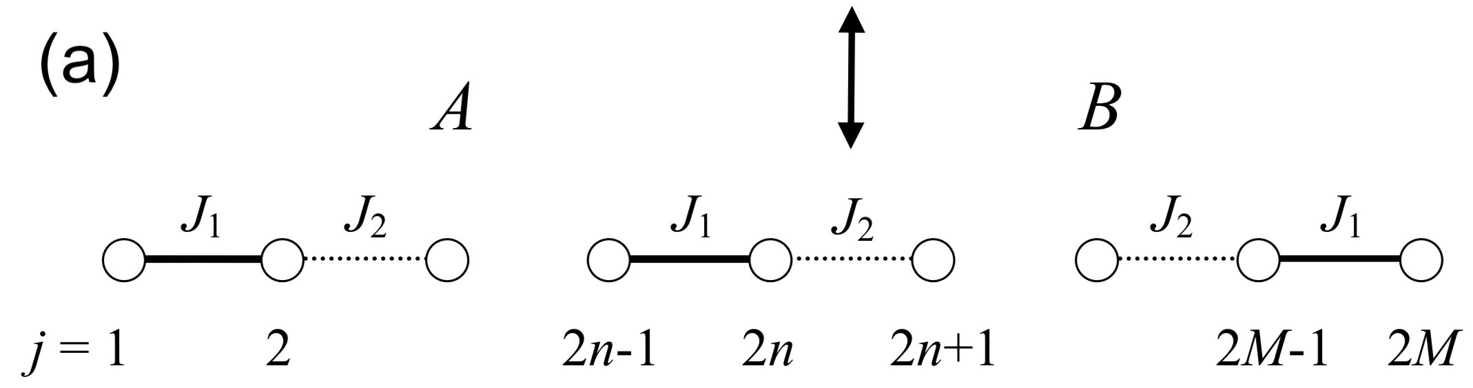
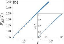
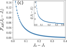
Figure 1: (a) Bipartition of the Kitaev spin chain into subparts $A$ and $B$. (b) DMRG results for bipartite fluctuations as a function of the subsystem length $l_{A}=L$ at the critical point: $\mathcal{F}_{AB}=\alpha\ln L+\mathcal{O}(1)$ with $\alpha=0.95/\pi^{2}$. The entanglement entropy is shown in the inset: $\mathcal{S}=(c/6)\ln L+\mathcal{O}(1)$ with central charge $c=0.49$. (c) Bipartite fluctuations as a function of $\Delta=|J_{2}-J_{1}|$ (here, $(J_{1},J_{2})<0$ such that the strong bonds occur on the $x$-link). The inset shows the correlation length $\xi=0.20\times\Delta^{-\nu}$ with $\nu=0.94$. For the gapped phase, we set $L_{\text{total}}=1000$.

III.2 Results on fluctuations

III.2.1 Logarithmic growth

Below, we focus on $\mathcal{F}_{AB}$, which defines the fluctuations between two subsystems (2.5) associated to bond-bond correlations (3.9). Here the valence bond fluctuations $\mathcal{F}_{AB}$ also appear as the effective non-vanishing lower bound for mutual information (2.10).

Fig. 1 (a) depicts the bipartition we choose for the spin chain with subsystem lengths $l_{A}=l_{B}={L_{\text{total}}}/2=L$. A direct lattice summation in Appendix B leads to

$$\mathcal{F}_{AB}=\begin{cases}({1}/{\pi^{2}})\ln l_{A}+({1}/{\pi^{2}})\left(\gamma+\ln 2-{1}/{2}\right),J_{1}=J_{2};\\ c_{1}\ln\xi+c_{2}e^{-1}\left(2\xi^{2}-\xi\right)+\mathcal{O}\left(1\right),\quad\ {|J_{1}|>|J_{2}|}.\end{cases}$$ (3.14)

with $\gamma\simeq 0.57721$ the Euler constant. On the contrary, $\mathcal{F}_{A}$ always contains a higher order scaling linear in $l_{A}$.

Our findings (3.14) are confirmed by DMRG simulations. At the gapless point $J_{1}=J_{2}$ shown in Fig. 1 (b), we observe in $\mathcal{F}_{AB}$ a logarithmic scaling with respect to the length of subregion $A$: $\mathcal{F}_{AB}\propto\ln l_{A}$. Roughly, one can identify this term by taking the 1D integral of the bond correlation $I(i,j)$ in Eq. (3.10). Moreover, the pre-factor $\alpha/\pi^{2}$ is recovered with $\alpha=0.95$. Here, the fact that $\alpha$ reproduces central charge $c=1$ of the dual lattice, is in agreement with the free bond fermion representation [61].

Fig. 1 (c) further probes the gapped region. When $|J_{1}|\gg|J_{2}|$, we check that $\mathcal{F}_{AB}$ goes to zero reflecting the crystallization of the dimers. Slowly closing the gap $\Delta$, near the phase transition point, $|c_{1}|\gg|c_{2}|$. we check that the logarithmic behavior $\propto\ln\xi$ dominates in $\mathcal{F}_{AB}$.

III.2.2 Relation to entanglement entropy

It is interesting to go beyond the lower bound and reveal the relation between $\mathcal{F}_{AB}$ and the original entanglement entropy. Deep in the gapped phase driven by $|J_{1}|\gg|J_{2}|$, eigenstates are formed on strong $x$-links. $\mathcal{S}_{A}$ vanishes accordingly when the boundary is set on the weak $y$-link (see Fig. 1, a). By increasing $|J_{2}|$, long-range entanglement emerges among the dimers, which is accompanied by a logarithmic growth in entropy associated to the correlation length

$$\mathcal{S}_{A}\propto\ln\xi.$$ (3.15)

The same response is observed in valence bond fluctuations $\mathcal{F}_{AB}$ of the gapped region.

Meanwhile, the entropy reaches its maximum when the gap closes at $J_{1}=J_{2}$. Suppose the critical chain is finite with open boundaries, the entropy is proven to show the universal behaviour [62, 59]:

$$\mathcal{S}_{A}=\frac{c}{6}\ln l_{A}+2g+s_{1},$$ (3.16)

where $g$ counts the boundary entropy and $s_{1}$ stands for a non-universal constant. In inset of Fig. 1 (b), from DMRG, we check that the central charge extracted from the entropy (3.16) reads: $c=0.49\sim 1/2$. It can be understood from the fact that after the Jordan-Wigner transformation, half of the spin degrees of freedom are disentangled from the Hamiltonian (3.3) by decoupling all $d$-Majorana fermions.

At the gapless point, both $\mathcal{F}_{AB}$ and $\mathcal{S}_{A}$ then share a logarithmic growth with subsystem size typical of (critical) conformal field theories in one dimension. Related to this finding, we would like to address the following comment: to evaluate the valence bond fluctuations we diagonalize the spectrum in momentum space in the $\psi$ basis, whereas the entanglement entropy reflects the real space degrees of freedom on the original lattice. This justifies why in our calculations the central charge $c=1$ is revealed in the valence bond fluctuations, whereas the central charge $c=1/2$ is observed in the entanglement entropy.

We establish that in both the gapped and gapless phases of one-dimensional Kitaev spin liquids, there is an identical scaling rule between the valence bond fluctuations and the entanglement entropy

$$\mathcal{F}_{AB}\sim\mathcal{S}_{A}.$$ (3.17)

IV Model on the honeycomb lattice

As discussed briefly in Sec. II.3 and as will be described below, on the two-dimensional honeycomb lattice, due to the protection of $0$-flux configurations in the ground state, the two-spin correlator also vanishes beyond nearest neighbors in all phases [24]. The valence bond correlator, however, preserves flux pairs in neighboring plaquettes and supports gapless fermion excitations. Although Ref. [47] finds numerically that it exhibits a power-law decay in the gapless phase and an exponential decay in gapped phases, the valence bond correlator itself does not locate precisely the phase transition (see Fig. 2, a). It motivates us to develop an approach of evaluating its global fluctuations on a bipartite lattice. The enhanced features in fluctuations come intrinsically from the spatial dependence and anisotropy of the local bond correlator.

We demonstrate below that the valence bond fluctuations and the entanglement entropy allow us to locate quite accurately the phases and quantum phase transitions in the two-dimensional Kitaev honeycomb model [21].

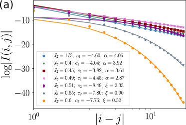
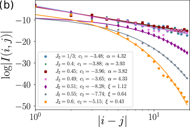
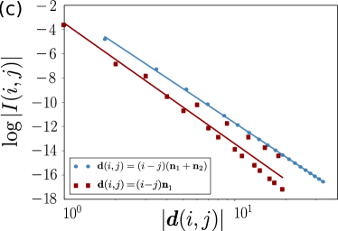
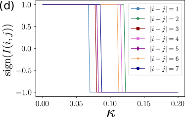
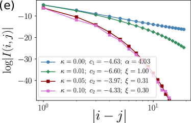
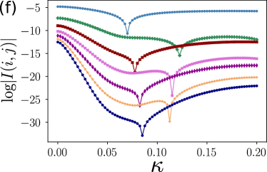
Figure 2: (a), (b) and (c): valence bond correlation functions for different phases in the pure Kitaev honeycomb model. The coupling constants are chosen according to $J_{x}=J_{y},\sum_{a}J_{a}=1$ and we take the total system size as $N=L\times L=100\times 100$. While the gapped phase ($J_{z}>0.5$) exhibits an exponential decay in bond correlators: $\log|I(i,j)|=c_{2}-|i-j|/\xi$, the gapless intermediate phase ($J_{z}\leq 0.5$) supports a power-law decay: $\log|I(i,j)|=c_{1}-\alpha\log|i-j|$. The relative vector is set along the direction $\textbf{d}(i,j)=\vec{r}_{i}-\vec{r}_{j}$: (a) $\textbf{d}(i,j)=(i-j)(\vec{n}_{1}+\vec{n}_{2})=(0,\sqrt{3}(i-j))$; (b) $\textbf{d}(i,j)=(i-j)\vec{n}_{1}=((i-j)/2,\sqrt{3}(i-j)/2)$. (c) Anisotropy effects in the gapless phase ($J_{x}=J_{y}=J_{z}=1/3$). Valence bond correlator for the intermediate phase in the presence of a uniform magnetic field $[111]$: (d) Sign change; (e) Exponential decay for the finite field; (f) Absolute amplitude with varied magnetic strengths. Here we present the case $J_{x}=J_{y}=J_{z}=1/3$. The direction of the relative vector is chosen on $\textbf{d}(i,j)=(i-j)(\vec{n}_{1}+\vec{n}_{2})$.

IV.1 Majorana representation

We start from the Hamiltonian $\mathcal{H}=-\sum_{\langle ij\rangle_{a}}J_{a}\sigma_{i}^{a}\sigma_{j}^{a}$, under the perturbation $\mathcal{V}=-\sum_{j}h_{a}\sigma_{j}^{a}$, where $\langle ij\rangle$ represents two nearest-neighbor sites, forming the bonds and $a=x,y,z$ denotes one of three different Ising couplings assigned onto them (see Fig. 3, a). When $|h_{a}|\ll|J_{a}|$, the cubic term in perturbation theory breaks time-reversal symmetry, and the effective Hamiltonian is simplified to [21]

$$\mathcal{H}=-\sum_{\langle ij\rangle_{a}}J_{a}\sigma_{i}^{a}\sigma_{j}^{a}-\kappa\sum_{\langle\langle ik\rangle\rangle}\sigma_{i}^{a}\sigma_{j}^{c}\sigma_{k}^{b}.$$ (4.1)

Here $\kappa\sim h_{x}h_{y}h_{z}/(J_{a}J_{b})$ and $\langle\langle ik\rangle\rangle$ describes next-nearest neighbors $i$ and $k$ connected by site $j$. Below, we study the effect of $\kappa$ in the perturbative regime of Eq. (4.1) where $\kappa\ll J_{x}+J_{y}+J_{z}$.

On the honeycomb lattice, one can write spin operators in terms of four Majorana fermions per site [21]:

$$\sigma_{j}^{a}=ic_{j}c_{j}^{a},$$ (4.2)

with the constraint for a physical state

$$D_{j}=c_{j}c_{j}^{x}c_{j}^{y}c_{j}^{z}=1.$$ (4.3)

Here, $c_{j}$ are matter Majorana fermion operators determining the fermionic spectrum and $c_{j}^{a}$ belong to gauge Majorana fermions which in the ground state, can be fixed artificially. Noticing that $[ic_{i}^{a}c_{j}^{a},\mathcal{H}]=0$ and $(ic_{i}^{a}c_{j}^{a})^{2}=1$, we choose the gauge $u_{\langle ij\rangle_{a}}=ic_{i}^{a}c_{j}^{a}:=+1$ for $i$ in sublattice $\{1\}$, as depicted in Fig. 3 (a), such that the total flux in the plaquette becomes zero consistent with Lieb’s theorem [63]. The definition of two sub-lattices, named $1$ and $2$ in Fig. 3 (a), follow the one-dimensional situation and the presence of two inequivalent bonds in a (zig-zag) given direction.

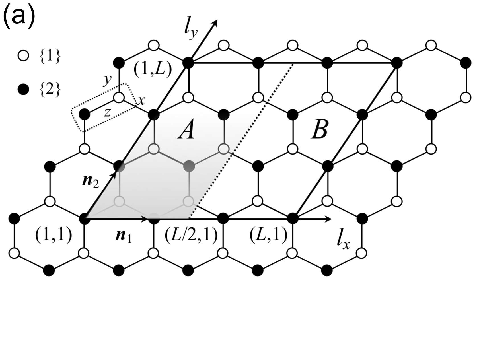
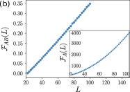
Figure 3: (a) Bipartition into two subsystems $A$ and $B$. The parallelogram is formed with unit vectors: $\vec{n}_{1}=(1/2,\sqrt{3}/2)$, $\vec{n}_{2}=(-1/2,\sqrt{3}/2)$. The bond observable is chosen on each $z$-link (dashed box); (b) Scaling of $\mathcal{F}_{AB}={\alpha}_{\mathcal{F}}L+\mathcal{O}(\ln L)$ in the gapless intermediate phase $J_{x}=J_{y}=J_{z}$. We obtain numerically ${\alpha}_{\mathcal{F}}=0.00449$. The inset shows the scaling of $\mathcal{F}_{A}=\alpha L^{2}+\beta L+\mathcal{O}(\ln L)$ with $\alpha=0.391,\beta=0.0129$.

The effective Hamiltonian [21] then presents a quadratic form in terms of $c_{j}$ as in one dimension (3.3):

$$\mathcal{H}=\sum_{\langle ij\rangle_{a}}iJ_{a}c_{i}c_{j}+\sum_{\langle\langle ik\rangle\rangle}i\kappa c_{i}c_{k}.$$ (4.4)

To obtain the eigenvectors, again it is more convenient to use the basis of complex bond fermions:

$$\psi_{r}=\frac{1}{2}(c_{r,1}+ic_{r,2})$$ (4.5)

with $r$ the unit cell coordinate defined on the $z$-links and $\{1,2\}$ the sublattice index. In momentum space, one arrives at a similar form of Hamiltonian as Eq. (3.5) with matrix elements

$$\xi_{\vec{k}}=\mathfrak{Re}{f(\vec{k})},\quad\Delta_{\vec{k}}=-g(\vec{k})+i\mathfrak{Im}f(\vec{k}).$$ (4.6)

Here, $f(\vec{k})$ and $g(\vec{k})$ are functions of the form

$$f(\vec{k})=J_{x}e^{i\vec{k}\cdot\vec{n}_{1}}+J_{y}e^{i\vec{k}\cdot\vec{n}_{2}}+J_{z},$$

$$g(\vec{k})=2\kappa[\sin(\vec{k}\cdot\vec{n}_{1})+\sin(\vec{k}\cdot(\vec{n}_{2}-\vec{n}_{1})-\sin(\vec{k}\cdot\vec{n}_{2})]$$ (4.7)

with two unit vectors $\vec{n}_{1}=(1/2,\sqrt{3}/2)$ and $\vec{n}_{2}=(-1/2,\sqrt{3}/2)$ shown in Fig. 3 (a). We check that the energy spectrum obtained from Eqs. (3.7), (4.6) and (4.7) reveals a gapless intermediate semi-metal phase  [21]

$$|J_{a}|\leq|J_{b}|+|J_{c}|$$ (4.8)

where $(a,b,c)$ involve all permutations of $(x,y,z)$.

IV.2 Valence bond correlator

For the honeycomb lattice, we choose to measure the valence bond correlator onto the $z$-links, as compared to the $x$-links used for the one-dimensional chain in Sec. III:

$$Q_{i}=\sigma_{i,1}^{z}\sigma_{i,2}^{z}=-ic_{i,1}c_{i,2}u_{\langle i_{1}i_{2}\rangle_{z}}:=-ic_{i,1}c_{i,2}.$$ (4.9)

Since any physical observable is independent of a specific gauge [24], in the last equality, we can adapt our gauge choice for the gauge Majorana fermions. One thus sees the bond correlator probes the matter Majorana fermions without disturbing the gauge part.

On the contrary, a single spin operator $\sigma_{j,1}^{z}=ic_{j,1}c_{j,1}^{z}$ influences the gauge structure [24]. Defining the bond gauge fermion $\chi=(c_{j,1}^{z}+ic_{j,2}^{z})/2$, we find that the number operator $N_{\chi}=\chi^{\dagger}\chi=(u_{\langle j_{1}j_{2}\rangle_{z}}+1)/2$ takes the value $1$ and $0$ depending on the gauge choice of $u_{\langle j_{1}j_{2}\rangle_{z}}=\pm 1$. In either gauge, $\sigma_{j,1}^{z}=ic_{j,1}(\chi^{\dagger}+\chi)$ changes the occupation number of the bond gauge fermion $\chi$. It is equivalent to flip the linking number $u_{\langle j_{1}j_{2}\rangle_{z}}$ to $-u_{\langle j_{1}j_{2}\rangle_{z}}$ and excite one $\pi$-flux pair in two neighbouring plaquettes. Therefore, the two-spin correlation is totally suppressed by the static $\mathbb{Z}_{2}$ gauge background beyond nearest neighbours (the latter case goes back to the measurement on a single bond).

Next, we focus on the local structure of the non-vanishing valence bond correlation. From Wick’s theorem, one obtains a compact form

$$I(i,j)=-\sum_{\vec{k},\vec{q}}\frac{e^{i(\vec{k}+\vec{q})\cdot(\vec{r}_{j}-\vec{r}_{i})}[g(\vec{k})g(\vec{q})+f(\vec{k})^{*}f(\vec{q})]}{N^{2}\sqrt{(\xi_{\vec{k}}^{2}+|\Delta_{\vec{k}}|^{2})(\xi_{\vec{q}}^{2}+|\Delta_{\vec{q}}|^{2})}},$$ (4.10)

with $N$ the total number of lattice unit cells.

IV.2.1 Zero field

In the absence of magnetic field $\kappa=0$, $I(i,j)$ has no singularities in the three gapped Abelian phases, therefore this results in an exponential decay of $I(i,j)$. In the intermediate gapless semi-metal phase, singularities appear at two Dirac points $\pm\vec{k}^{*}$.

We first look at the behavior of bond correlations in the gapless region. A detailed analysis of the asymptotic behavior of $I(i,j)$ at long distances can be found in Appendix C. Performing an expansion around the two Dirac points similar to the $p_{x}+ip_{y}$ superconductor [64], we recover a power-law decay [47]

$$I(i,j)=\frac{\widetilde{c}_{1}}{r^{4}},$$ (4.11)

and establish that the $\widetilde{c}_{1}$ coefficient depends on the cutoff function $t(\Lambda)$ and on the anisotropic function $Y(\vec{r})$. More precisely,

$$\widetilde{c}_{1}=t^{2}(\Lambda)\cdot Y(\vec{r}),$$

$$Y(\vec{r})=\cos^{2}(\vec{k}^{*}\cdot\vec{r})-\cos^{2}(\theta^{*}).$$ (4.12)

Here, $\theta^{*}$ is the angle between the vectors $\vec{r}=\vec{r}_{i}-\vec{r}_{j}$ and $\vec{k}^{*}$. The space variable $r$ refers to $|\vec{r}_{i}-\vec{r}_{j}|$.

We can start from the simplest case by making the directions of $\vec{r}$ and $\vec{k}^{*}$ perpendicular to each other: $\vec{r}_{\perp}=\vec{r}_{j}-\vec{r}_{i}=(j-i)(\vec{n}_{1}+\vec{n}_{2})$. The spatial oscillations disappear in the bond correlator with $Y(\vec{r}_{\perp})=1$. Our analytic expression becomes consistent with the numerical fitting results of Ref. [47]. Shown in Fig. 2 (a), it supports a smooth curve of $I(i,j)$ revealing the $r^{-4}$ scaling in the gapless region ($J_{z}<0.5$).

We can derive a more precise analysis. At the gapless point $J_{x}=J_{y}=J_{z}=1/3$, in Appendix. C we derive the expression for the cutoff function

$$t(\Lambda)=\frac{\sqrt{3}}{2\pi}\int_{0}^{\Lambda}J_{1}(k)kdk,$$ (4.13)

where inside the integral $J_{1}(k)$ denotes the Bessel function of the first kind. Here, the cutoff $\Lambda=\xi r$ can be further approximated by setting the radius of the momentum integration $\xi=1$ and taking $r\simeq r_{\text{max}}$ to be the total system size $L=100$. Analytically, we obtain $\log|I(i,j)|=c_{1}-\alpha\log|i-j|$ with $c_{1}=\left.\log(\widetilde{c}_{1}/9)\right|_{\Lambda=100}=-4.63$, $\alpha=4$. Here, $``\log"$ is equivalent to the natural logarithm with the base ${e}$. It recovers well the numerical fitting result (see Fig. 2, a): $c_{1}=-4.60,\alpha=4.06$.

It is important to stress that Ref. [47] has not pointed out the role of the anisotropic $Y$-function. Once shifted to other directions $Y(\vec{r})\neq$ cst, $c_{1}=\log(|\cos^{2}(\vec{k}^{*}\cdot\vec{r})-\cos^{2}(\theta^{*})|)-4.63.$ Accordingly, as verified by Fig. 2 (b) and (c), the sampling points of $\log|I(i,j)|$ along the non-perpenticular direction oscillate rapidly. We also emphasize here the forms of $\tilde{c}_{1}$ and the anisotropic $Y$-function in Eq. (4.12) remain true for the whole gapless region. Later, we will study these anisotropic effects on the bipartite fluctuations in relation with Fig. 4.

For the gapped phase, on the other hand, from numerics $I(i,j)$ follows an exponential decay with a fast decreasing correlation length shown in Fig. 2 (a). Meanwhile, in Fig. 2 (b), one observes less anisotropy effects in the gapped region.

It may be relevant to mention that once the gapless intermediate phase is subject to a magnetic field along the $\hat{z}$ direction, an identical power-law behavior (including the same angular dependence) emerges in the dynamical correlation function [25]:

$$g(t,\vec{r})=\langle\sigma_{r}^{z}(t)\sigma_{0}^{z}(0)\rangle-\langle\sigma_{0}^{z}(0)\rangle^{2}$$

$$\simeq\frac{64h_{z}^{2}}{\pi^{2}h_{0}^{2}}\frac{r^{2}(\cos^{2}(\vec{k}^{*}\cdot\vec{r})-\cos^{2}(\theta^{*}))-3(Jt)^{2}\cos^{2}(\vec{k}^{*}\cdot\vec{r})}{(r^{2}-3(Jt)^{2})^{3}}$$ (4.14)

where $h_{z}$ is the strength of the magnetic field and the parameter $h_{0}$ can be estimated as $h_{0}\sim J$. We find at long distances and at a finite time,

$$t\ll r\to\infty,\quad\frac{g(t,\vec{r})}{I(\vec{r},\kappa=0)}\propto\text{cst}.$$ (4.15)

Both observables are proportional to the density-density correlation function of the bond fermions $\psi_{r}$ in (4.5).

IV.2.2 Small finite field

We further study the effects of a small uniform magnetic field on the bond correlation in the intermediate phase. For simplicity, we take $J_{x}=J_{y}=J_{z}=J=1/3$.

When $0<\kappa\ll J$, a gap opens and the valence bond correlator in Fig. 2 (e) now reveals an exponential decay, similar to three gapped spin liquid phases. Yet its sign changes from positive to negative when increasing the strength of the magnetic field (see Fig. 2, d). Consequently, in Fig. 2 (f) we observe an enhancement in the amplitude of bond correlation functions once the magnetic field is sufficiently large.

We find that this sign change originates from the competition between the Ising interactions and the external magnetic field. For $\kappa\neq 0$, the valence bond correlator (4.10) can be expressed in an alternative form

$$I(i,j) =F(\vec{r})^{2}-G(\vec{r})^{2},$$

$$F(\vec{r}) =\frac{1}{N}\sum_{k}e^{i\vec{k}\cdot{\vec{r}}}\frac{f(k)^{*}}{\sqrt{\xi_{k}^{2}+|\Delta_{k}|^{2}}},$$

$$G(\vec{r}) =\frac{1}{N}\sum_{k}e^{i\vec{k}\cdot{\vec{r}}}\frac{g(k)}{\sqrt{\xi_{k}^{2}+|\Delta_{k}|^{2}}}.$$ (4.16)

While the Ising interactions give a positive contribution to the bond correlators, the external magnetic field gives a negative one.

Changing the strength of the external magnetic field $\kappa$, it is verified that

$$\quad\text{Sign}\left(\frac{\partial I(i,j)}{\partial\kappa}\right)=\text{Sign}(-\kappa),$$ (4.17)

as ${\partial_{\kappa}I(i,j)}=2[{\partial_{\kappa}F(\vec{r})}\cdot F(\vec{r})-{\partial_{\kappa}G(\vec{r})}\cdot G(\vec{r})]$ and

$$\frac{\partial F(\vec{r})}{\partial\kappa} =-\frac{1}{N}\sum_{k}e^{i\vec{k}\cdot{\vec{r}}}\frac{f(k)^{*}g(k)^{2}}{\kappa(\xi_{k}^{2}+|\Delta_{k}|^{2})^{3/2}},$$

$$\frac{\partial G(\vec{r})}{\partial\kappa} =\frac{1}{N}\sum_{k}e^{i\vec{k}\cdot{\vec{r}}}\frac{g(k)|f(k)|^{2}}{\kappa(\xi_{k}^{2}+|\Delta_{k}|^{2})^{3/2}}.$$ (4.18)

When $\kappa>0$, the derivative of $I(i,j)$ is always negative.

The monotonically decreasing bond correlation function is expected to cross zero around the point where the strengths of the Ising interactions and the magnetic field are comparable. We can roughly estimate the crossover point by starting from a relatively small $\kappa$ parameter. In this circumstance, $I(i,j)$ is still governed by an expansion $|\delta\vec{k}|\in\Omega(0,1)$ around two original Dirac points $\pm\vec{k}^{*}$. The denominator in Eq. (4.16) turns out to be

$$E_{k}=\sqrt{\xi_{k}^{2}+|\Delta_{k}|^{2}}=3\sqrt{3}|\kappa|\sqrt{1+(\lambda k)^{2}}.$$ (4.19)

When the parameter $\lambda=J/(6\kappa)>1$, $\kappa<\kappa_{c}=0.055$, the $F(\vec{r})^{2}$ term arising from the Ising interactions is dominant and $I(i,j)$ keeps a positive sign. Otherwise $\lambda\ll 1$, $\kappa\gg\kappa_{c}$, then the $-G(\vec{r})^{2}$ term from the external magnetic field grows steadily and has the tendency to drive $I(i,j)$ negative. In accordance with the numerical calculations shown in Fig. 2 (d) and (f), for different distances, all crossover points where $I(i,j)$ changes sign are located at $\kappa>\kappa_{c}$.

IV.3 Results on fluctuations

IV.3.1 Area law

Next, to gain some intuition on the behavior of bipartite fluctuations, in Appendix D we perform analytically the lattice summation by assuming an isotropic form of $I(i,j)$, namely with $Y(\vec{r})=1$.

Given a bipartition on the honeycomb lattice represented in Fig. 3 (a), we first derive a general scaling form for fluctuations within an arbitrary region $\Omega=l_{x}\times l_{y}$

$$I(r)\propto\frac{1}{r^{\alpha}},\quad\mathcal{F}_{\Omega}\propto\begin{cases}L^{4},\quad\alpha=0;\\ L^{3},\quad\alpha=1;\\ L^{2},\quad\alpha\geq 2,\end{cases}$$ (4.20)

with $l_{x}$ and $l_{y}$ of the same order as $L$.

For the Kitaev honeycomb model, from Sec. IV.2 we see the valence bond correlator reveals a power law decay ($\alpha=4$) in the gapless phase and an exponential decay ($\alpha\to\infty$) in the gapped phases. Therefore, in all phases $\mathcal{F}_{A}$ shows the volume law: $\mathcal{F}_{A}\propto L^{2}=\mathcal{V}$. As usual, we can extract $\mathcal{F}_{AB}$ from the equality (2.6): $\left|\mathcal{F}_{A\cup B}-\mathcal{F}_{A}-\mathcal{F}_{B}\right|/2$. With a subsystem size $A=B={(L/2)}\times L$, it is noticeable that the volume term vanishes after the subtraction, leading to an area law in $\mathcal{F}_{AB}\propto L=\mathcal{A}$, where $\mathcal{A}$ refers then to an area.

Meanwhile, under the $Y$-isotropic form assumption, we establish in Appendix D the linear scaling factor of valence bond fluctuations in different phases:

$$\mathcal{F}_{AB}={\alpha}_{\mathcal{F}}L+\mathcal{O}(\ln L).$$ (4.21)

In the gapless phase, we obtain ${\alpha}_{\mathcal{F}}=3.84\tilde{c}_{1}$ where $\tilde{c}_{1}$ denotes the constant coefficient in the bond correlator (4.11) for a given set of $J_{a}$’s. In a gapped phase, we obtain ${\alpha}_{\mathcal{F}}\propto\xi^{3}$ with $\xi$ the correlation length. This approach then implies that with a rapidly growing correlation length, ${\alpha}_{\mathcal{F}}$ must reach a maximum when undergoing a quantum phase transition from a gapped phase into the gapless intermediate regime (see Fig. 4, a).

Numerically, we check these results by the method of finite-size scaling which starts from the anisotropic form (4.10) of the function $I(i,j)$. The exact anisotropic numerical calculations agree well with our previous $Y$-isotropic form approximation. In Fig. 3 (b), we recover the linear scaling of $\mathcal{F}_{AB}$ in the gapless phase ($J_{x}=J_{y}=J_{z}$). The inset shows the scaling of $\mathcal{F}_{A}$, where the leading-order $L^{2}$ term ($0.391$) is dominated by the on-site bond fluctuations ($0.362$, from Eq. (D13)). Since these on-site contributions are later subtracted, $\mathcal{F}_{AB}$ contains more information about the entanglement properties.

IV.3.2 Peak structure in linear scaling factor

Shown in Fig. 4 (a), we continue our study by extracting numerically the linear scaling factor of valence bond fluctuations from different regimes of the phase diagram. A peak structure centered at the quantum phase transition line is observed. While the gapped region can be understood from the simultaneous evolution with the correlation length ($\alpha_{\mathcal{F}}\propto\xi^{3}$), we check that the anisotropy effects in the $Y$-function are responsible for the decrease of $\alpha_{\mathcal{F}}$ when the system goes deeper into the gapless phase.

It is noted that after the double summation in $\mathcal{F}_{AB}$ (2.5), the bond fluctuations around the boundary (or domain wall) between two subsystems become the major contribution. Therefore, we can focus on the short-range behavior of the anisotropic factor $Y(\vec{r})$ in the bond correlator (4.12) along the direction perpendicular to the boundary. Illustrated by Fig. 4 (b), at short distances, $Y(\vec{r})$ reaches the maximum value when $J_{z}$ evolves to the phase transition line. Consequently, the amplitude of the linear scaling ${\alpha}_{\mathcal{F}}$ in $\mathcal{F}_{AB}$ would drop when we decrease $J_{z}$ in the gapless phase.

Fig. 4 (c) also includes the development of the linear scaling factor ${\alpha}_{\mathcal{F}}$ with different magnetic strengths. The signature of the peak structure in ${\alpha}_{\mathcal{F}}$ across the phase transition line is robust against small fields ($\kappa\leq 0.10$). By increasing $\kappa$, the gap is enlarged. The anisotropic effects of the $Y(\vec{r})$ function originally dominant in the gapless region become reduced significantly, thus making the cusp of $\alpha_{F}$ more smooth. Stronger magnetic field effects are discussed qualitatively in Sec. V.1.

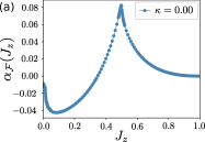
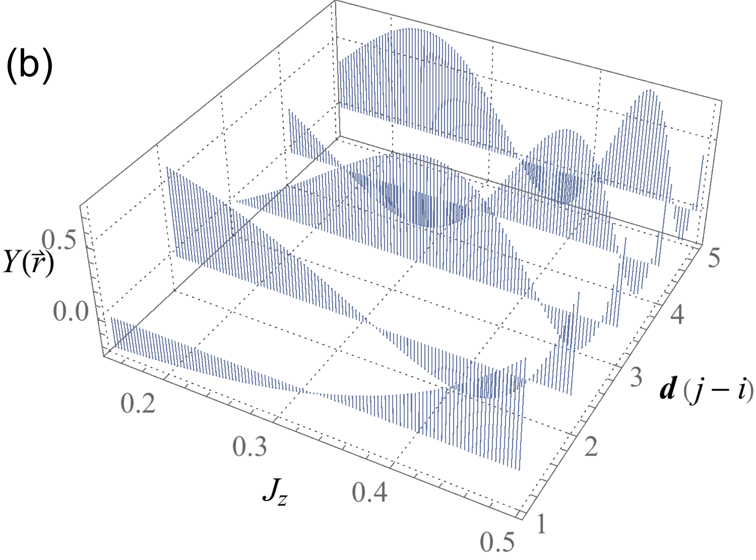
Figure 4: (a) Prefactor ${\alpha}_{\mathcal{F}}$ of the linear term in the bipartite fluctuations $\mathcal{F}_{AB}$ for the gapless intermediate phase ($J_{z}\leq 0.5$) and the gapped phase with bonds polarized in the $z$ direction $(J_{z}>0.5)$ of the Kitaev honeycomb model. (b) Anisotropic function $Y(\vec{r})$ in the gapless phase. The relative vector is set along the direction of $\vec{n}_{1}$ (perpendicular to the boundary between subsystems $A$ and $B$): $\vec{r}=\vec{r}_{j}-\vec{r}_{i}=\textbf{d}(j-i)=(j-i)\vec{n}_{1}$. Effects of a small uniform magnetic field on the linear scaling factors of valence bond fluctuations and the Fermi entropy : (c) Prefactor ${\alpha}_{\mathcal{F}}$ in $\mathcal{F}_{AB}$; (d) Prefactor ${\alpha_{\mathcal{S}}}$ in $\mathcal{S}_{F}$. In four plots, the conventions for coupling constants $J_{x}=J_{y}$ and $J_{x}+J_{y}+J_{z}=1$ are adopted. And the magnetic field strength $\kappa$ varies in the range $[0.00,0.10]$. The calculation of $\mathcal{F}_{AB}$ is performed on a finite lattice cluster $\Omega=A\cup B=L\times L$ with the total length $L$ varying from $30$ to $100$. For the finite-size scaling of $\mathcal{S}_{F}$, on the other hand, the length of the zigzag boundary across $x$-links is taken as $L=N_{x}\in[40,100]$.

IV.3.3 Relation to Fermion entropy

Now, we address the behavior of the entanglement entropy in the Kitaev model. As pointed out in Ref. [30], the total entanglement entropy of the Kitaev honeycomb model consists of two pieces: the gauge field part $\mathcal{S}_{G}=(L-1)\ln 2$ and the fermionic contribution

$$\mathcal{S}_{F}={\alpha}_{\mathcal{S}}L+\mathcal{O}(1).$$ (4.22)

Since the measurement of valence bond fluctuations preserves the $\mathbb{Z}_{2}$ gauge field structure, $\mathcal{F}_{AB}$ probes the entanglement properties of the fermion sector. Fortunately, $\mathcal{S}_{F}$ is responsible for all the essential differences between the Abelian and non-Abelian phases.

We then extract the linear factor ${\alpha}_{\mathcal{S}}$ from $\mathcal{S}_{F}$ following the methods of Refs. [65, 30]. For completeness, we refer the readers to Appendix E where some details on the numerical approach to evaluate the Fermi entropy are presented. It is found that in a small magnetic field $\kappa=0.01$, the linear scaling factor ${\alpha}_{\mathcal{S}}$ shares the same response as ${\alpha}_{\mathcal{F}}$ across the phase transition line shown in Fig. 4 (d). On top of that, once the magnetic field strength is increased, the peak structure of $\alpha_{\mathcal{S}}$ in Fermi entropy disappears slightly more quickly than the one in bond fluctuations. In addition, it is relevant to observe that $\alpha_{\mathcal{S}}$ remains zero for $J_{z}>0.5$. Another interesting observation is that as a function of $J_{z}$, the magnitudes of $\alpha_{\mathcal{F}}$ and $\alpha_{\mathcal{S}}$ vary approximately in the same range $[0,0.10]$.

To summarize, in two dimensions, we also find that valence bond fluctuations and the entanglement entropy of the Fermi sector show the same area law scaling in all phases:

$$\mathcal{F}_{AB}\sim S_{F}.$$ (4.23)

Moreover, their linear scaling factors act as signatures to characterize quantum phase transitions between the Abelian and non-Abelian phases in the Kitaev honeycomb model.

V Concluding remarks

In this final section, we would like to make brief remarks about the effects of stronger magnetic fields on the gapless phase of the Kitaev honeycomb model. Two scenarios are presently discussed in the literature: one with excitations of flux pairs [37, 27], and the other with a transition to another type of gapless spin liquid with U(1) symmetry [48]. We will propose possible responses from the valence bond fluctuations respectively.

Afterwards, a comparison with the Néel state supported by antiferromagnetic Heisenberg interactions will give us additional insights with regard to the application in quantum materials.

V.1 Influence of Perturbations

V.1.1 Perturbed Kitaev QSLs with gauge-flux pairs

For the Kitaev materials in a gapless spin liquid state, two types of gaps have been observed in the presence of a small tilted magnetic field [37]

$$\Delta=\Delta_{v}+\Delta_{f}.$$ (5.1)

Here, $\Delta_{v}$ denotes the gap from the creation of a pair of fluxes (or visons) and $\Delta_{f}\propto h_{x}h_{y}h_{z}$ refers to the one induced by one matter Majorana fermion excitation. Our previous analysis of Sec. IV remains valid as long as $\Delta_{v}\gg\Delta_{f}$.

In Ref. [27], it was suggested that one can construct an exact perturbed ground state with even number of virtual fluxes by a unitary mapping $U$ from the unperturbed state $|\varphi_{0}\rangle$: $|\varphi\rangle=U|\varphi_{0}\rangle$. The transformed spin operator takes the form [27]

$$U^{\dagger}\sigma_{i}^{a}U=iZc_{i}c_{i}^{a}+\cdots+f_{ijk}^{a}ic_{j}c_{k}+\cdots,$$ (5.2)

with $Z=1,f=0$ for the pure Kitaev model and $Z<1,f\neq 0$ in the presence of perturbations. The nonzero $f$ parameters open a Majorana fermion gap instantaneously.

One immediately notices for the valence bond operator $Q_{i}=\sigma_{i,1}^{z}\sigma_{i,2}^{z}$, that the leading order contribution turns into

$$U^{\dagger}Q_{i}U=Z^{2}(-ic_{i,1}c_{i,2})+(\text{quartic terms}).$$ (5.3)

Concerning the gauge Majorana fermions $c_{i}^{a}$, we have used the gauge convention form $u_{\langle i_{1}i_{2}\rangle_{z}}=+1$ and all others being zero, acting on the unperturbed state. The first term in the transformed bond operator (5.3) has a rescaling factor $Z^{2}$. It leads to a $r^{-4}$ decay in valence bond correlation $I(i,j)=\langle Q_{i}Q_{j}\rangle_{c}$ within the distance shorter than the correlation length ($r<\xi$). The second part contains products of four matter Majorana fermions, which then result in much faster decays in bond correlations, for instance $r^{-6}$ and $r^{-8}$ over short distances.

Neglecting these higher order corrections arising from the $f$-decomposition and taking into account the general scaling rule on honeycomb lattice (4.20), we establish that the valence bond fluctuations still show an area law

$$\mathcal{F}^{\text{VB}}_{AB,\text{perturbed}}=\alpha_{\mathcal{F},\text{perturbed}}\cdot L+\mathcal{O}(\ln L),$$ (5.4)

The linear scaling factor is rescaled according to

$$\alpha_{\mathcal{F},\text{perturbed}}\simeq Z^{4}\alpha_{\mathcal{F},0},$$ (5.5)

where $\alpha_{\mathcal{F},0}$ denotes the prefactor of the linear term reminiscent of the zero-flux Kitaev spin liquids. Based on Sec. IV.3, we thus find

$$\alpha_{\mathcal{F},0}\propto\xi_{f}^{3}\propto\Delta_{f}^{-3}.$$ (5.6)

With excitations of flux pairs, the linear scaling factor now combines two pieces of information: the vison gap $\Delta_{v}$ determining the amplitude of $Z^{4}$ and the Majorana fermion gap $\Delta_{f}$ coming into play through $\alpha_{\mathcal{F},0}$.

It may be relevant to mention that the two-spin fluctuations become already nonzero in the perturbed limit. From Eq. (5.2), one gets contributions from the $f$-sector of Majorana fermions. Accompanied by an exponential decay in the spin-spin correlation, we obtain

$$\mathcal{F}^{\text{TS}}_{AB,\text{perturbed}}=\alpha^{\text{TS}}_{\mathcal{F}}\cdot L+\mathcal{O}(\ln L),$$ (5.7)

where

$$\alpha^{\text{TS}}_{\mathcal{F}}\propto(f^{z})^{2}\cdot\Delta_{f}^{-3}.$$ (5.8)

When $\Delta_{v}\gg\Delta_{f}$, no excitation of fluxes is allowed. When $f^{z}\to 0$, $\alpha^{\text{TS}}_{\mathcal{F}}\to 0$, we check the result of vanishing two-spin fluctuations in the solvable limit (2.25).

V.1.2 Transition to U(1) gapless spin liquids

If one continues to increase the strength of the uniform magnetic field, from numerical simulations [48], while the Kitaev ferromagnet produces a trivial polarized phase (PL), the Kitaev antiferromagnet might give rise to an intermediate phase supporting U(1) gapless spin liquids (GSL).

In the PL phase, there is no correlation between two subsystems and both the two-spin and valence bond fluctuations vanish

$$\mathcal{F}^{\text{TS/VB}}_{AB,\text{PL}}=0.$$ (5.9)

For the GSL phase in the Kitaev antiferromagnet, one can assume a gapless spinon Fermi surface coupled to a U(1) gauge field. In an effective picture of complex Abrikosov fermions [48], a spin operator is mapped onto the product of fermions $2\vec{S}=f_{\alpha}^{\dagger}\vec{\sigma}_{\alpha\beta}f_{\beta}$, with spin index $\alpha,\beta=\uparrow,\downarrow$ and a U(1) symmetry $f_{\alpha}^{\dagger}\to e^{i\theta}f_{\alpha}^{\dagger}$. From this perspective, the spin and bond correlations follow power-law decays ($r^{-4}$, $r^{-8}$ respectively) in the gapless phase. We predict that an “enhancement” might be observed in the prefactor of the area-law bipartitie fluctuations

$$\mathcal{F}^{\text{TS/VB}}_{AB,\text{GSL}}=\alpha^{\text{TS/VB}}_{\mathcal{F},\text{GSL}}\cdot L+\mathcal{O}(\ln L).$$ (5.10)

The existence of a similar peak structure in $\alpha_{\mathcal{F}}$ between the gapped Kitaev spin liquids and U(1) gapless spin liquids is possible and can be tested numerically in the future.

V.2 Comparison with the Néel phase

In the end, to make a closer link with quantum materials, it is perhaps useful to compare the obtained behavior of bond-bond correlation functions from the ones of the two-dimensional Heisenberg model, i.e., of a Néel ordered phase subject to spin-wave excitations. When antiferromagnetic Heisenberg interactions are dominant, the modified spin-wave theory predicts that a staggered magnetic field is required to stabilize the Néel state at zero temperature for finite lattices [66, 56].

Performing a spin-wave analysis in Appendix F, then we find that the same valence bond correlation shows:

$$I(i,j)=c_{0}+{c_{1}}{r}^{-1}$$ (5.11)

with $c_{0}=0.131$ and $c_{1}=0.141$.

As a result, the bipartite fluctuations now follow a volume square law:

$$\mathcal{F}_{AB}\propto L^{4},$$ (5.12)

arising from the non-vanishing long-range correlation of $c_{0}$. Measuring the precise leading order scalings then allows to probe the phase, Kitaev spin liquid versus Néel state, of a two-dimensional quantum material. We emphasize here that the entanglement entropy of the Néel state still reveals an area law [56], as in the Kitaev spin model. The violation of the lower bound (2.10) originates from the finite-size regularization procedure taken in the modified spin-wave theory.

V.3 Conclusion

To summarize, we have found a general relation between the valence bond fluctuations and the entanglement entropy of the Kitaev spin model in one and two dimensions. Valence bond fluctuations appear as a relevant tool to identify phases and phase transitions of Majorana magnetic quantum systems. Application to three-dimensional systems [67, 68] can be studied in the future.

Appendix A SU(2) quantum spin systems

Here, we evaluate the two-spin fluctuations and valence bond fluctuations for the SU(2)-symmetric quantum spin models both in one and two dimensions. We differentiate two cases: the one where the singlets resonate with equal weights and the other where they decay exponentially over distance.

A.1 Finite-size singlet state

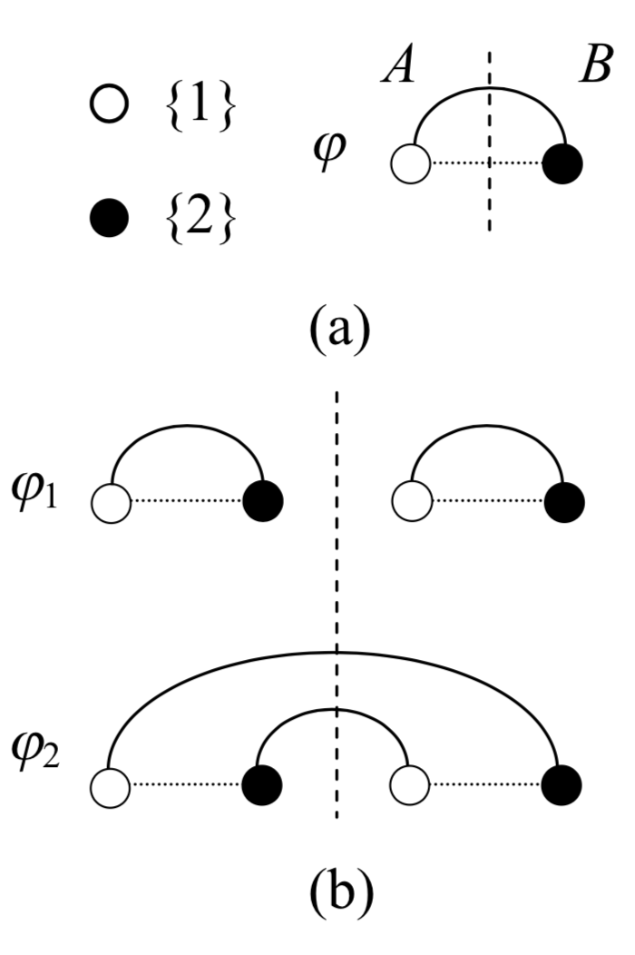
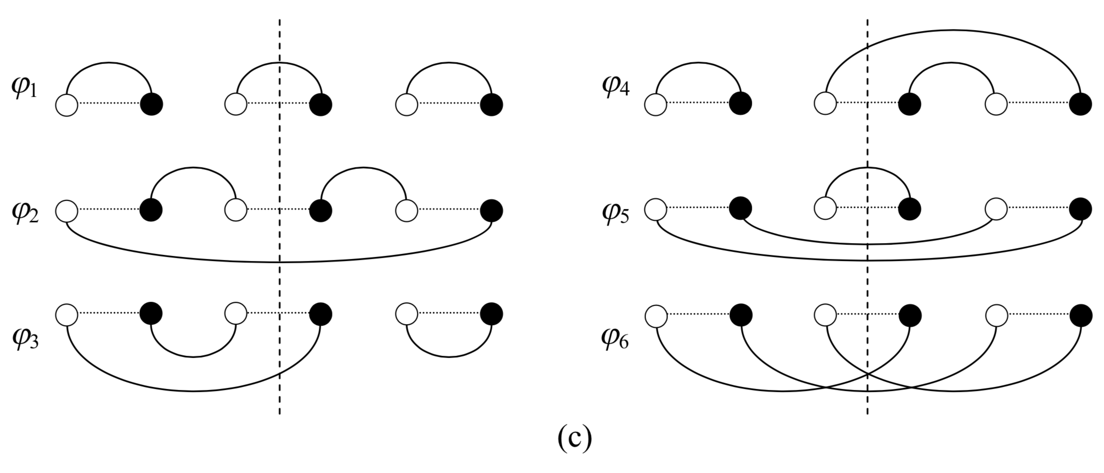
Figure 5: Possible pairing configurations for the $N$-site singlet state: (a) $N=2$; (b) $N=4$; (c) $N=6$. We allow for entanglement on different sublattices. Two sites paired by a solid curve form a local valence bond state: $|\frown\ \rangle_{\overline{(i,1)(j,2)}}=(|\uparrow_{i,1}\rangle|\downarrow_{j,2}\rangle-|\downarrow_{i,1}\rangle|\uparrow_{j,2}\rangle)/\sqrt{2}$.

We start from one dimension. Fig. 5 shows all the pairing states $\{|\varphi\rangle_{i}\}$ for $N=2,4,6$-site singlets. $N$ can also be interpreted as the maximum resonating range of the VB states on an infinite chain. As $N\to\infty$, the system approaches the critical point.

When $N=2$, we have a unique singlet state $|\Phi_{0}\rangle=|\varphi\rangle$ shown in Fig. 5 (a). Once the boundary between two subsystems $A$ and $B$ is set on the bond, one recovers immediately $\mathcal{F}^{\text{TS}}=1$, $\mathcal{F}^{\text{VB}}=0$, $\mathcal{S}^{\text{VB}}=\ln 2$ and the relation $\mathcal{S}^{\text{VB}}/\mathcal{F}^{\text{TS}}=\ln 2$. Nevertheless, if the boundary is off the bond, $\mathcal{F}^{\text{TS}}=\mathcal{F}^{\text{VB}}=\mathcal{S}^{\text{VB}}=0$. In the following analysis, we always keep the size of the two subsystems to be the same.

For $N=4$ in Fig. 5 (b), a simple normalized singlet state reads $|\Phi_{0}\rangle=(|\varphi_{1}\rangle+|\varphi_{2}\rangle)/\sqrt{3}$ with an overlap between two pairings $\langle\varphi_{1}|\varphi_{2}\rangle=1/2$. Also, we have assumed the system has equal chance to stay in each pairing state. Then

$$\mathcal{S}^{\text{VB}}=\frac{0+2\ln 2/\sqrt{3}}{2/\sqrt{3}}=\ln 2,$$

$$\mathcal{F}^{\text{TS}}=0+\left(\frac{1}{\sqrt{3}}\right)^{2}\cdot 2=\frac{2}{3},\quad\mathcal{F}^{\text{VB}}=0+\left(\frac{1}{\sqrt{3}}\right)^{2}=\frac{1}{3}.$$ (A1)

We find a new relation

$$\frac{\mathcal{S}^{\text{VB}}}{\mathcal{F}^{\text{TS}}+\mathcal{F}^{\text{VB}}}=\ln 2.$$ (A2)

Yet Eq. (A2) does not hold if $N>4$. We can check the case $N=6$ shown in Fig. 5 (c). The system allows $(N/2)!=6$ pairing configurations and the normalization factor $\mathcal{D}$ becomes larger than 6 on account of the overlaps:

$$|\Phi_{0}\rangle=\frac{1}{\sqrt{\mathcal{D}}}\sum_{p=1}^{n_{p}=6}|\varphi_{p}\rangle,\quad\mathcal{D}=\sum_{p,p^{\prime}=1}^{n_{p}=6}\langle\varphi_{p}|\varphi_{p^{\prime}}\rangle=18.$$ (A3)

While each $|\varphi_{p}\rangle$ is responsible for $\mathcal{S}^{\text{VB}}$ and $\mathcal{F}^{\text{TS}}$, only $|\varphi_{p=4,5}\rangle$ contribute to $\mathcal{F}^{\text{VB}}$.

$$\mathcal{S}^{\text{VB}}=\frac{10\cdot(\ln 2)/\sqrt{\mathcal{D}}}{6/\sqrt{\mathcal{D}}}=\frac{5\ln 2}{3},$$

$$\mathcal{F}^{\text{TS}}=\left(\frac{1}{\sqrt{\mathcal{D}}}\right)^{2}\cdot 10=\frac{5}{9},\quad\mathcal{F}^{\text{VB}}=\left(\frac{1}{\sqrt{\mathcal{D}}}\right)^{2}\cdot 2=\frac{1}{9}.$$ (A4)

Therefore, ${\mathcal{S}^{\text{VB}}}/({\mathcal{F}^{\text{TS}}+\mathcal{F}^{\text{VB}}})=({5}/{2})\ln 2>\ln 2$.

In two dimensions, for a gapped VB state composed of $N$-site singlets, the generalized result becomes

$$\mathcal{S}^{\text{VB}}\propto\ln 2\cdot n,\quad\frac{\mathcal{S}^{\text{VB}}}{\mathcal{F}^{\text{TS}}+\mathcal{F}^{\text{VB}}}\geq\ln 2.$$ (A5)

$n$ denotes the number of singlets that the boundary crosses. Both relations above take the equality $``="$ if the resonating range $N\leq 4$. Meanwhile, we recover the area law of bipartite fluctuations

$$\mathcal{F}^{\text{TS}}=f^{\text{TS}}(N)\cdot n,\quad\mathcal{F}^{\text{VB}}=f^{\text{VB}}(N)\cdot n,$$ (A6)

where the coefficients depend on the size of the singlets. For instance, we have $f^{\text{TS}}(2)=1,f^{\text{VB}}(2)=0;f^{\text{TS}}(4)=2/3,f^{\text{VB}}(4)=1/3;f^{\text{TS}}(6)=5/9,f^{\text{VB}}(6)=1/9$.

A.2 General singlet state

Next, we consider a gapped system where the singlet bonds decay exponentially with distance, and $\mathcal{F}^{\text{TS}}$ and $\mathcal{F}^{\text{VB}}$ still show an area law as the entanglement entropy.

We first test the 1D case. A general VB state can be constructed as

$$|\Phi_{0}\rangle=\frac{1}{\sqrt{\mathcal{D}}}\sum_{p}\prod_{\overline{(i,1)(j,2)}\in p}\frac{e^{-|i-j|/\xi}}{\sqrt{2}}(|\uparrow_{i1}\rangle|\downarrow_{j2}\rangle-|\downarrow_{i1}\rangle|\uparrow_{j2}\rangle)$$ (A7)

where $\xi$ stands for the correlation length of dimers. The probability of two sites $(i,1)$ and $(j,2)$ being paired reads

$$P(\overline{(i,1)(j,2)})=P(|i-j|)=ce^{-2|i-j|/\xi}.$$ (A8)

Correspondingly, on a chain with a total length $2L$ ($1\ll\xi\ll L$),

$$\mathcal{F}^{\text{TS}}_{\text{1D}} =\sum_{(i,\alpha)\in A}\sum_{(j,\beta)\in B}P(|i-j|)$$

$$=\sum_{i=1}^{L/2}\sum_{j=L/2+1}^{L}P(|i-j|)\cdot 2=\frac{c}{2}\xi^{2}+\mathcal{O}(\xi),$$ (A9)

$$\mathcal{F}^{\text{VB}}_{\text{1D}} =\sum_{i=1}^{L/2}\sum_{j=L/2+1}^{L}P(|i-j|)^{2}=\frac{c^{2}}{16}\xi^{2}+\mathcal{O}(\xi).$$ (A10)

$\mathcal{F}^{\text{TS/VB}}_{\text{1D}}$ becomes a constant proportional to the square of the correlation length.

In two dimensions, one can apply the general scaling rule of Appendix D.1 on $\mathcal{F}^{\text{TS/VB}}=\sum_{i\in A,j\in B}I(i,j)$. Since the correlators $I(i,j)$ follow an exponential decay (as in one dimension), the bipartite fluctuations between two subsystems should be proportional to the perimeter $x$ of the boundary

$$\mathcal{F}^{\text{TS/VB}}_{\text{2D}}=b^{\text{TS/VB}}\cdot x+\mathcal{O}(x).$$ (A11)

Hence, we find a similar area law in the two types of fluctuations as for the VB entanglement entropy in (2.17).

Appendix B Kitaev spin chain

Here, we give a mathematical proof of Eq. (3.14).

B.1 Quantum critical point $J_{1}=J_{2}$

For the critical Kitaev spin chain at the gapless point $J_{1}=J_{2}$, we first evaluate the bipartite fluctuation within subregion $A$:

$$\mathcal{F}_{A}=\sum_{i,j\in A}I(i,j)=\sum_{i,j\in A}I(\left|i-j\right|).$$ (B1)

The bond correlation depends only on the difference of two variables. One can thus convert the double sum into a single sum through

$$\sum_{i,j\in A}I(\left|i-j\right|)=I(0)l_{A}+2\sum_{k=1}^{l_{A}}(l_{A}-k)I(k).$$ (B2)

From the expression (3.10) of $I(k)$: $1/[{\pi^{2}}(k^{2}-1/4)]$ for $k\neq 0$; $1-4/\pi^{2}$ for $k=0$, we get

$$\sum_{k=1}^{l_{A}}I(k) =\frac{4}{\pi^{2}}\sum_{k=1}^{l_{A}}\frac{1}{4k^{2}-1}$$

$$=\frac{2}{\pi^{2}}\left(1-\frac{1}{2l_{A}+1}\right)=\frac{2}{\pi^{2}}+\mathcal{O}(l_{A}^{-1}),$$

$$\sum_{k=1}^{l_{A}}kI(k) =\frac{1}{\pi^{2}}\sum_{k=1}^{l_{A}}2k\left(\frac{1}{2k-1}-\frac{1}{2k+1}\right)$$

$$=\frac{1}{\pi^{2}}\sum_{k=1}^{2l_{A}}\left(\frac{k+1}{k}-\frac{k-1}{k}\right)\sigma_{k}-\frac{l_{A}}{2l_{A}+1}$$

$$=\frac{2}{\pi^{2}}\sum_{k=1}^{2l_{A}}\frac{\sigma_{k}}{k}-\frac{l_{A}}{2l_{A}+1},$$ (B3)

with $\sigma_{k}=1$ for $k=\text{odd}$ and $\sigma_{k}=0$ for $k=\text{even}$. It is convenient to re-express the finite sum in terms of the difference of two infinite sums

$$\sum_{k=1}^{2l_{A}}\frac{\sigma_{k}}{k} =\sum^{\infty}_{k=1}\frac{\sigma_{k}}{k}-\frac{\sigma_{k+2l_{A}}}{k+2l_{A}}$$

$$=\sum_{k=1}^{\infty}\left(\frac{1}{k}-\frac{1}{2k}\right)-\left(\frac{1}{k+2l_{A}}-\frac{1}{2k+2l_{A}}\right).$$ (B4)

In the second equality, we have also used the relation: $(\text{odd terms})=(\text{all terms})-(\text{even terms})$. Now we can apply the properties of the digamma function, which shares the series representation related to the Euler’s constant $\gamma\simeq 0.57721$, as well as the asymptotic expansion

$$\psi(x)=-\gamma+\sum_{k=1}^{\infty}\left(\frac{1}{k}-\frac{1}{k+x-1}\right),$$

$$\psi(x\to\infty)=\ln x-\frac{1}{2x}-\frac{1}{12x^{2}}+\mathcal{O}(x^{-4}).$$ (B5)

Therefore,

$$\sum_{k=1}^{2l_{A}}\frac{\sigma_{k}}{k} =\psi(2l_{A}+1)+\gamma-\frac{1}{2}\left(\psi(l_{A}+1)+\gamma\right)$$

$$=\frac{1}{2}\ln l_{A}+\frac{\gamma}{2}+\ln 2+\mathcal{O}(l_{A}^{-1}).$$ (B6)

For a bipartition $l_{A}=l_{B}=L/2$, we then get the critical scaling of $\mathcal{F}_{A}$ and at the same time, $\mathcal{F}_{AB}$ from their relation (2.6)

$$\mathcal{F}_{A} =l_{A}-\frac{2}{\pi^{2}}\ln l_{A}-\frac{2}{\pi^{2}}\left(\gamma+2\ln 2-\frac{1}{2}\right)+\mathcal{O}(l_{A}^{-1}),$$

$$\mathcal{F}_{AB} =\frac{1}{\pi^{2}}\ln l_{A}+\frac{1}{\pi^{2}}\left(\gamma+\ln 2-\frac{1}{2}\right)+\mathcal{O}(l_{A}^{-1}).$$ (B7)

B.2 Gapped regime $|J_{1}|>|J_{2}|$

We continue to study the gapped phase of the Kitaev spin chain with negative exchanges such that $|J_{1}|>|J_{2}|$, such that the strong bonds occur on the $x$-links. In Eqs. (3.12) and (3.13), we predict that the bond correlator behaves as $I(i,j)=c_{1}|i-j|^{-2}$ for $|i-j|\leq\xi$ and $I(i,j)=c_{2}e^{-|i-j|/\xi}$ for $|i-j|>\xi$, with a correlation length $\xi\sim\left|J_{2}-J_{1}\right|^{-1}$. For $1<\xi<l_{A}=l_{B}=L/2$, the valence bond fluctuations between two subregions become

$$\mathcal{F}_{AB} =\sum_{i=1}^{L/2}\sum_{j=L/2+1}^{L}I(i,j)$$

$$=\sum_{k=1}^{\xi}k\frac{c_{1}}{k^{2}}+\sum_{k=\xi+1}^{L/2}kc_{2}e^{-\frac{k}{\xi}}+\sum_{k=L/2+1}^{L}\left(L-k\right)c_{2}e^{-\frac{k}{\xi}}.$$ (B8)

Approximating the single summation by an integral and supposing $\xi\ll L$, one obtains

$$\mathcal{F}_{AB}=c_{1}\ln\xi+c_{2}e^{-1}\left(2\xi^{2}-\xi\right)+\mathcal{O}\left(1\right).$$ (B9)

Appendix C Asymptotic form of bond correlator in the intermediate gapless phase

Here, we derive the power-law behavior of bond correlation functions in the intermediate gapless spin liquid phase of the Kitaev honeycomb model. We assume a simple case where three Ising couplings share the same strength: $J_{x}=J_{y}=J_{z}=J$.

When $\kappa=0$, the valence bond correlator (4.10) can be re-expressed as the product of two sums

$$I(i,j) =-\langle-ic_{i,1}c_{j,2}\rangle\langle-ic_{j,1}c_{i,2}\rangle,$$

$$\langle-ic_{i,1}c_{j,2}\rangle =\frac{1}{N}\sum_{\vec{k}}e^{i\vec{k}\cdot(\vec{r}_{j}-\vec{r}_{i})}\frac{f(k)^{*}}{|f(k)|},$$

$$\langle-ic_{j,1}c_{i,2}\rangle =\frac{1}{N}\sum_{\vec{q}}e^{-i\vec{q}\cdot(\vec{r}_{j}-\vec{r}_{i})}\frac{f(q)^{*}}{|f(q)|}.$$ (C1)

The main contribution comes from the two Dirac points $\pm\vec{k}^{*}=\pm(k_{x}^{*},k_{y}^{*})=\pm({4\pi}/{3},0)$ which satisfy $|f(\pm\vec{k}^{*})|=0$. It allows us to approximate the summation by an expansion around each Dirac point within a small radius $\xi$: $\vec{k}\in\Omega(\pm\vec{k}^{*},\xi)$.

For the first sum in Eq. (C1), around one Dirac point $\vec{k}^{*}=(4\pi/3,0)$ we get

$$\frac{f(\vec{k})^{*}}{|f(\vec{k})|}=-\cos\theta^{\prime}+i\sin\theta^{\prime}.$$ (C2)

Here $\theta^{\prime}$ is the angle between the relative vector around the Dirac cone $\delta\vec{k}=\vec{k}-\vec{k}^{*}$ and the $x$ axis. It is clear to see that $I(i,j)$ is anisotropic. To simplify the exponential, we denote the direction of the two unit cells as $\vec{r}=\vec{r}_{j}-\vec{r}_{i}=(r\cos{\theta^{*}},r\sin{\theta^{*}})$ with $\theta^{*}$ the angle between vectors $\vec{r}$ and $\vec{k}^{*}$. Then,

$$e^{i\vec{k}\cdot(\vec{r}_{j}-\vec{r}_{i})}=e^{i\vec{k}^{*}\cdot\vec{r}}e^{i\delta\vec{k}\cdot\vec{r}}=e^{i\vec{k}^{*}\cdot\vec{r}}e^{i{\delta k}r\cos\theta},$$ (C3)

with $\theta$ the relative angle between $\delta\vec{k}$ and $\vec{r}_{j}-\vec{r}_{i}$.

Now we can evaluate the summation by taking the continuum limit

$$\langle-ic_{i,1}c_{j,2}\rangle_{\vec{k}^{*}}= \frac{(-1)}{(2\pi)^{2}}\cdot\frac{\sqrt{3}}{2}\int_{0}^{\xi}kdk\int_{0}^{2\pi}e^{ikr\cos{\theta}}$$

$$\times e^{i(\vec{k}^{*}\cdot\vec{r}-\theta^{*})}(\cos\theta+i\sin\theta)d\theta.$$ (C4)

The factor $2$ comes from the contribution of two Dirac points. The other factor $\sqrt{3}/2$ originates from a change of basis from $dk_{1}dk_{2}$ in the Brillouin zone (with unit vectors $\vec{n}_{1}$ and $\vec{n}_{2}$) to $dk_{x}dk_{y}$. We have also used the relation $\theta+\theta^{\prime}=\theta^{*}$.

Via a change of variables $k^{\prime}=kr$, one reaches

$$\langle-ic_{i,1}c_{j,2}\rangle_{\vec{k}^{*}} =-\frac{\sqrt{3}}{8\pi^{2}}e^{i(\vec{k}^{*}\cdot\vec{r}-\theta^{*})}\int_{0}^{\Lambda}\frac{kdk}{r^{2}}\int_{0}^{2\pi}\cos{\theta}e^{ik\cos{\theta}}d\theta$$

$$=-\frac{t(\Lambda)}{2r^{2}}ie^{i(\vec{k}^{*}\cdot\vec{r}-\theta^{*})},$$ (C5)

where $t(\Lambda)=\sqrt{3}/(2\pi)\cdot\int_{0}^{\Lambda}J_{1}(k)kdk$ with a cutoff $\Lambda=\xi r$ and inside the integral $J_{1}(k)$ denotes the Bessel function of the first kind.

A similar expansion around the other Dirac point $-\vec{k}^{*}=(-4\pi/3,0)$ would give an additional phase factor $e^{i(-\vec{k}^{*}\cdot\vec{r}-(\pi-\theta^{*}))}$. Thus, the total contribution reads

$$\langle-ic_{i,1}c_{j,2}\rangle =\langle-ic_{i,1}c_{j,2}\rangle_{\vec{k}^{*}}+\langle-ic_{i,1}c_{j,2}\rangle_{-\vec{k}^{*}}$$

$$=\frac{t(\Lambda)}{r^{2}}\sin(\vec{k}^{*}\cdot\vec{r}-\theta^{*}).$$ (C6)

For the second sum in Eq. (C1), we only need to change $\vec{r}$ to $-\vec{r}$ and adjust the relative angle from $\theta^{*}$ to $\theta^{*}-\pi$:

$$\langle-ic_{j,1}c_{i,2}\rangle=\frac{t(\Lambda)}{r^{2}}\sin(\vec{k}^{*}\cdot\vec{r}+\theta^{*}).$$ (C7)

Combining Eqs. (C1), (C6) and (C7), we then recover the $r^{-4}$ scaling of the bond correlator in the gapless phase [47]:

$$I(i,j)=\frac{\widetilde{c}_{1}}{r^{4}}.$$ (C8)

Furthermore, from our calculations the amplitude $\widetilde{c}_{1}$ retrieves an anisotropic factor $Y(\vec{r})$:

$$\widetilde{c}_{1}=t^{2}(\Lambda)\cdot Y(\vec{r}),$$

$$Y(\vec{r})=\cos^{2}(\vec{k}^{*}\cdot\vec{r})-\cos^{2}(\theta^{*}).$$ (C9)

One can also verify that the forms of $\tilde{c}_{1}$ and of the anisotropic $Y$-function in Eq. (C9) are valid for the whole gapless region.

Appendix D Bipartite fluctuations on honeycomb geometry

We evaluate here the bipartite fluctuations on the honeycomb lattice, involving the lattice summation.

D.1 General scaling rule

Consider a bipartition on the honeycomb lattice shown in Fig. 3 (a). The parallelogram is expanded by two unit vectors $\vec{n}_{1}=(1/2,\sqrt{3}/2)$ and ${\vec{n}_{2}}=(-1/2,\sqrt{3}/2)$ with a total size $\Omega=l_{x}\times l_{y}$ and the subsystems are chosen as $A=B=(l_{x}/2)\times l_{y}={(L/2)}\times L$. For convenience, we adopt new coordinates $\vec{r}=x\vec{n}_{1}+y\vec{n}_{2}:x=1,2,\dots,l_{x},y=1,2,\dots,l_{y}$. The summation in the bipartite fluctuations can then be re-expressed into

$$\mathcal{F}_{\Omega}=\sum_{\vec{r},\vec{r}^{\prime}\in\Omega}I(\vec{r}^{\prime}-\vec{r})=\sum_{x,x^{\prime}=1}^{l_{x}}\sum_{y,y^{\prime}=1}^{l_{y}}I(x^{\prime}-x,y^{\prime}-y).$$ (D1)

To derive general scaling arguments in a ‘simple’ way, we only consider the case where $I(\vec{r})$ is an isotropic function of the distance $|\vec{r}|=\sqrt{x^{2}+xy+y^{2}}$. By analogy to Eq. (B2), a relation between the double and single sums can be established

$$\sum_{x,x^{\prime}=1}^{l_{x}}I(x^{\prime}-x,y)$$

$$=l_{x}I(0,y)+\sum_{x=1}^{l_{x}}(l_{x}-x)\left[I(x,y)+I(-x,y)\right]$$ (D2)

and the same for $\sum_{y,y^{\prime}=1}^{l_{y}}I(x,y^{\prime}-y)$. Then the bipartite fluctuation function can be grouped into four parts:

$$\mathcal{F}_{\Omega}=l_{x}l_{y}I_{1}+l_{x}I_{2}+I_{y}I_{3}+I_{4},$$ (D3)

with

$$I_{1} =I(0,0)+2\sum_{x=1}^{l_{x}}I(x,0)+2\sum_{y=1}^{l_{y}}I(0,y)$$

$$\phantom{=}+2\sum_{x=1}^{l_{x}}\sum_{y=1}^{l_{y}}\left[I(x,y)+I(-x,y)\right],$$

$$I_{2} =-2\sum_{y=1}^{l_{y}}yI(0,y)-2\sum_{x=1}^{l_{x}}\sum_{y=1}^{l_{y}}y\left[I(x,y)+I(-x,y)\right],$$

$$I_{3} =-2\sum_{x=1}^{l_{x}}xI(x,0)-2\sum_{x=1}^{l_{x}}\sum_{y=1}^{l_{y}}x\left[I(x,y)+I(-x,y)\right],$$

$$I_{4} =2\sum_{x=1}^{l_{x}}\sum_{y=1}^{l_{y}}xy\left[I(x,y)+I(-x,y)\right].$$ (D4)

The dominant scaling terms in $\mathcal{F}_{\Omega}$ depend on the particular form of $I(r)$. Suppose a general case where $I(r)\propto r^{-\alpha}$ and $l_{x}$, $l_{y}$ are of the same order as $L$:

$$I_{1} \sim\mathcal{O}(1)+\mathcal{O}(\frac{1}{L^{\alpha-1}})+\mathcal{O}(\frac{1}{L^{\alpha-2}}),$$

$$I_{2},I_{3} \sim\mathcal{O}(1)+\mathcal{O}(\frac{1}{L^{\alpha-2}})+\mathcal{O}(\frac{1}{L^{\alpha-3}}),$$

$$I_{4} \sim\mathcal{O}(1)+\mathcal{O}{(\frac{1}{L^{\alpha-4}})},$$ (D5)

where $\mathcal{O}({1}/{L^{0}})\sim\mathcal{O}(\ln L)$. The leading-order scaling in $\mathcal{F}_{\Omega}$ becomes

$$I(r)\propto\frac{1}{r^{\alpha}},\quad\mathcal{F}_{\Omega}\propto\begin{cases}L^{4},\quad\alpha=0;\\ L^{3},\quad\alpha=1;\\ L^{2},\quad\alpha\geq 2.\end{cases}$$ (D6)

When $I(r)\propto e^{-r/\xi}$, $\alpha\to\infty$, $\mathcal{F}_{\Omega}$ still show the volume law: $\mathcal{F}_{\Omega}\propto L^{2}=\mathcal{V}$. Besides, after the subtraction: $\left|\mathcal{F}_{A\cup B}-\mathcal{F}_{A}-\mathcal{F}_{B}\right|/2$, while the higher order terms $L^{4}$ and $L^{3}$ survive in $\mathcal{F}_{AB}$ , the square term $L^{2}$ always vanishes, which leads to an area law in $\mathcal{F}_{AB}\propto L=\mathcal{A}$.

To evaluate $\mathcal{F}_{AB}$ more precisely, we are going to study next-leading order terms in $\mathcal{F}_{\Omega}$ case by case.

D.2 Kitaev model: the gapless phase

For the gapless phase of the Kitaev honeycomb model, first we consider an isotropic form of the valence bond correlator in Eq. (4.11)

$$I(x,y)=\frac{\tilde{c}_{1}}{(x^{2}+xy+y^{2})^{2}},$$ (D7)

where ${\tilde{c}_{1}}$ is a constant for a given $J_{z}\in[0,0.50]$ in our convention.

As $\alpha=4$, from the general scaling rule in Eq. (D5) we get $I_{i}(i=1,2,3)\propto\mathcal{O}(1)$ and $I_{4}\propto\mathcal{O}(\ln L)$. In particular, due to the convergence of the lattice summations in $I_{i}(i=1,2,3)$ in Eq. (D4), we can introduce a cutoff $l_{x}=l_{y}=\Lambda=10^{3}$ to approximate these pre-factors:

$$I_{1} \simeq I(0,0)+2\sum_{x=1}^{\Lambda}I(x,0)+2\sum_{y=1}^{\Lambda}I(0,y)$$

$$\phantom{=====}+2\sum_{x=1}^{\Lambda}\sum_{y=1}^{\Lambda}\left[I(x,y)+I(-x,y)\right]$$

$$=I(0)+7.32\widetilde{c}_{1},$$

$$I_{2} =I_{3}\simeq-2\sum_{y=1}^{\Lambda}yI(0,y)-2\sum_{x=1}^{\Lambda}\sum_{y=1}^{\Lambda}y\left[I(x,y)+I(-x,y)\right]$$

$$=-7.68\widetilde{c}_{1}.$$ (D8)

Here $I(0)$ denotes the on-site contribution and has the value

$$I(0)=1-\langle{Q}_{i}\rangle^{2}.$$ (D9)

$\langle{Q}_{i}\rangle=\langle\sigma^{z}_{i_{1}}\sigma^{z}_{i_{2}}\rangle$ represents the integral over the Brillouin zone:

$$\langle{Q}_{i}\rangle=(2\pi)^{-2}\int_{-\pi}^{\pi}\int_{-\pi}^{\pi}dk_{1}k_{2}\cos\theta(k_{1},k_{2}),$$ (D10)

with $\cos\theta(k_{1},k_{2})=a/\sqrt{a^{2}+b^{2}}$ and $f(k)=a+bi=J_{x}e^{ik_{1}}+J_{y}e^{ik_{2}}+J_{z}$. Combined with the general expression of $\mathcal{F}_{\Omega}$ in Eq. (D3), we arrive at

$$\mathcal{F}_{A} =\alpha L^{2}+\beta L+\mathcal{O}(\ln L),$$

$$\mathcal{F}_{AB} ={\alpha}_{\mathcal{F}}L+\mathcal{O}(\ln L),$$ (D11)

where

$$\alpha =I_{1}/2=I(0)/2+3.66\tilde{c}_{1},$$

$$\beta =3I_{2}/2=-11.5\tilde{c}_{1},$$

$${\alpha}_{\mathcal{F}} =|I_{2}|/2=3.84\widetilde{c}_{1}.$$ (D12)

In the special case $J_{x}=J_{y}=J_{z}=1/3$, we have

$$\langle Q_{i}\rangle\simeq 0.525,\quad I(0)/2\simeq 0.362.$$ (D13)

As indicated by the inset of Fig. 3 (b), the pre-factor of the $L^{2}$ term in $\mathcal{F}_{A}$ takes the value $\alpha=0.391$ close to $I(0)/2$. We conclude that the major contribution to $\mathcal{F}_{A}$ comes from the on-site interactions.

D.3 Kitaev model: the gapped phases

In the gapped phases, the bond correlation function decays exponentially and there is less anisotropy observed in Fig. 2 (b). We can safely start with an isotropic form

$$I(x,y)=c_{2}e^{-\sqrt{x^{2}+xy+y^{2}}/\xi}.$$ (D14)

For $\alpha=\infty$ in Eq. (D5), all of the amplitudes $I_{i}(i=1,2,3,4)\propto\mathcal{O}(1)$. Yet we can still relate them to the powers of the finite correlation length $\xi$. The following assumption is taken

$$\xi\sim L^{1/p},\qquad p\geq 5,$$ (D15)

such that when $n<5$,

$$L/\xi\to\infty,\quad 1/\xi\to 0,\quad\xi^{n}<L.$$ (D16)

Back to Eq. (D4), we can then replace the summations on the lattice with integrals

$$\sum_{x=1}^{l_{x}}I(x,0)=c_{2}\xi\int_{1/\xi}^{l_{x}/\xi}dxe^{-x}=c_{2}\xi\int_{0}^{\infty}dxe^{-x}=c_{2}\xi,$$

$$\sum_{y=1}^{l_{y}}yI(0,y)=c_{2}\xi^{2}\int_{0}^{\infty}ye^{-y}=c_{2}\xi^{2},$$

$$\sum_{x=1}^{l_{x}}\sum_{y=1}^{l_{y}}\left[I(x,y)+I(-x,y)\right]=3.63c_{2}\xi^{2}$$

$$=c_{2}\xi^{2}\int_{0}^{\infty}\int_{0}^{\infty}dxdy\left(e^{-\sqrt{x^{2}+xy+y^{2}}}+e^{-\sqrt{x^{2}-xy+y^{2}}}\right),$$

$$\sum_{x=1}^{l_{x}}\sum_{y=1}^{l_{y}}y\left[I(x,y)+I(-x,y)\right]=5.33c_{2}\xi^{3}$$

$$=c_{2}\xi^{3}\int_{0}^{\infty}\int_{0}^{\infty}dxdy\left(e^{-\sqrt{x^{2}+xy+y^{2}}}+e^{-\sqrt{x^{2}-xy+y^{2}}}\right)y,$$

$$\sum_{x=1}^{l_{x}}\sum_{y=1}^{l_{y}}xy\left[I(x,y)+I(-x,y)\right]=10.4c_{2}\xi^{4}$$

$$=c_{2}\xi^{4}\int_{0}^{\infty}\int_{0}^{\infty}dxdy\left(e^{-\sqrt{x^{2}+xy+y^{2}}}+e^{-\sqrt{x^{2}-xy+y^{2}}}\right)xy.$$ (D17)

The pre-factors now read

$$I_{1} =I(0)+7.26c_{2}\xi^{2}+4c_{2}\xi,$$

$$I_{2} =I_{3}=-10.7c_{2}\xi^{3}-2c_{2}\xi^{2},$$

$$I_{4} =20.8c_{2}\xi^{4}.$$ (D18)

Correspondingly, the bipartite fluctuations share the quadratic and linear forms respectively

$$\mathcal{F}_{A} =\alpha L^{2}+\beta L+\mathcal{O}(1),$$

$$\mathcal{F}_{AB} ={\alpha}_{\mathcal{F}}L+\mathcal{O}(1),$$ (D19)

with

$$\alpha =I_{1}/2\propto\xi^{2},$$

$$\beta =3I_{2}/2\propto\xi^{3},$$

$${\alpha}_{\mathcal{F}} =|I_{2}|/2\propto\xi^{3}.$$ (D20)

It indicates that in gapped phases, ${\alpha}_{\mathcal{F}}$ increases at the transition towards the intermediate gapless phase.

Appendix E Entanglement entropy of the Fermion sector

In this part, we extract the linear factor ${\alpha}_{\mathcal{S}}$ in $S_{F}$ applying the same numerical approach as in Refs. [65, 30]. The general idea is to map the total system $A\cup B$ on the honeycomb lattice of Fig. 3 (a) onto a torus geometry depicted in Fig. 6 (a). Periodic boundary conditions (PBC) are imposed along $X$ and $Y$ directions and the boundaries between subsystems now turn into two circles. Fig. 6 (a) also illustrates one of the two zigzag boundaries located on $x$-links. For this shape of the boundary, the generic Hamiltonian of subsystem $A$ reads

$$\mathcal{H}=\sum_{\langle jk\rangle\in A}iJ_{a}c_{j}c_{k}u_{\langle jk\rangle_{a}}+\sum_{\langle\langle jk\rangle\rangle\in A}i\kappa c_{j}c_{k}(-u_{\langle ji\rangle_{a}}u_{\langle ik\rangle_{b}}),$$ (E1)

where $\langle\ \ \rangle$ denotes the nearest-neighbor links and $\langle\langle\ \ \rangle\rangle$ the next-nearest-neighbor links. The gauge choice $u_{\langle jk\rangle_{a}}=+1,-u_{\langle ji\rangle_{a}}u_{\langle ik\rangle_{b}}=+1$ is manifested in the direction of the arrows from site $k$ to site $j$ in Fig. 6 (a).

Now along the $X$ direction, we go to the momentum space ($k_{x}=2m\pi/N_{x},m=0,1,\dots,N_{x}-1$) and Fourier transform the Hamiltonian (E1) into

$$\mathcal{H}=\sum_{k_{x}}\mathcal{C}^{\dagger}(k_{x})M(k_{x})\mathcal{C}(k_{x})$$ (E2)

in the basis of the matter Majorana fermions $\mathcal{C}^{\dagger}(k_{x})=\left(c_{-k_{x},1},c_{-k_{x},2}\right)$. The matrix takes the form

$$M(k_{x})=\begin{pmatrix}\alpha&is&-\beta&&&\\ -is^{*}&-\alpha&ir&\beta&&\\ -\beta&-ir&\alpha&is&-\beta&\\ &\beta&-is^{*}&-\alpha&ir&\cdots\\ &&-\beta&-ir&\alpha&\cdots\\ &&&&\cdots&\cdots\end{pmatrix},$$ (E3)

with matrix elements $r=-J_{x}$, $s=(J_{y}+J_{z})\cos(k_{x}/2)-i(J_{y}-J_{z})\sin(k_{x}/2)$, $\alpha=2\kappa\sin k_{x}$, $\beta=2\kappa\sin(k_{x}/2)$. It should be noted that the intrinsic structure of our $2N_{y}\times 2N_{y}$ Hamiltonian matrix $M(k_{x})$ is distinct from Ref. [30] where only one type of next-nearest-neighbor couplings $J^{\prime}$ is included. In our case, all three types of next-nearest-neighbor couplings between the matter Majorana fermions are taken into account, as they arise naturally from the effects of the uniform magnetic field [21]. Additionally, to be consistent with the bipartition we choose for $\mathcal{F}_{AB}$ in Fig. 3 (a), the boundary position has been switched from $z$-links in Ref. [30] to $x$-links.

The diagonalized Hamiltonian reads

$$\mathcal{H}=\sum_{n,k_{x}}\xi_{n}(k_{x})\left(\psi_{nk_{x}}^{\dagger}\psi_{nk_{x}}-\frac{1}{2}\right),$$ (E4)

where $n=1,\dots,2N_{y}$ and $\psi_{nk_{x}}$ represents the standard complex fermionic annihilation operators. For a free fermion system, the energy spectrum $\xi_{n}(k_{x})$ can be used to calculate the entanglement entropy [65]

$$\mathcal{S}(k_{x})=-\frac{1}{2}\sum_{n,k_{x}}\left[\lambda_{n}\log\lambda_{n}+(1-\lambda_{n})\log(1-\lambda_{n})\right](k_{x}).$$ (E5)

Here $\lambda_{n}(k_{x})=(e^{\beta\xi_{n}(k_{x})}+1)^{-1}$ denote the eigenvalues of the single-particle correlation function $\langle\psi^{\dagger}_{nk_{x}}\psi_{n^{\prime}k_{x}}\rangle$. It follows a Fermi-Dirac distribution with an inverse temperature $\beta=1/(k_{B}T)$. Fig. 6 (b) shows the numerical entanglement spectrum $\lambda_{n}(k_{x})$ for the non-Abelian and Abelian phases. We observe two gapless branches in the non-Abelian phase. These two modes are responsible for the peaks in entanglement entropy plotted in Fig. 6 (c). Both features disappear in the Abelian phase.

Since $\mathcal{S}_{F}=\sum_{k_{x}}\mathcal{S}(k_{x})$, through the summation of $\mathcal{S}(k_{x})$ in the momentum space followed by a finite-size scaling with respect to $N_{x}$, we are able to obtain the pre-factor $\alpha_{\mathcal{S}}$ of the linear term in $\mathcal{S}_{F}$. The results are shown in Fig. 4 (d) in the Article.

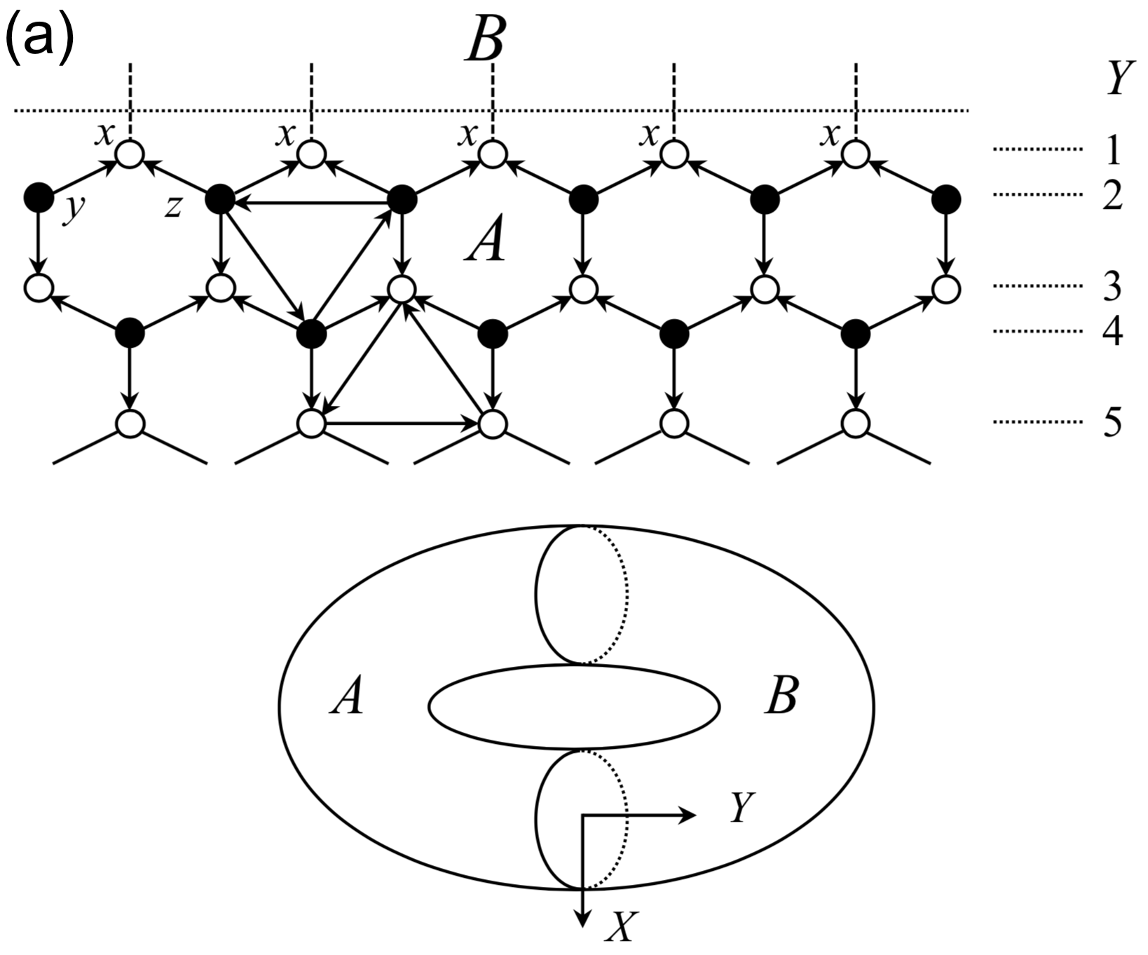
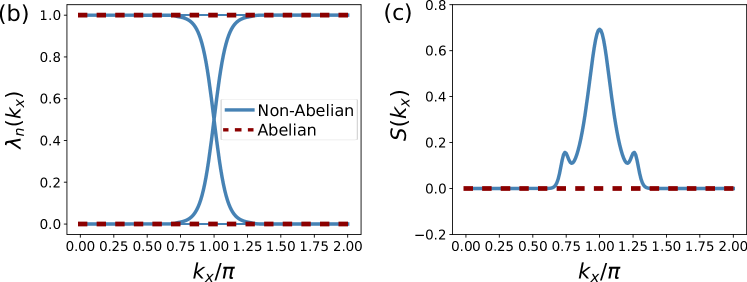
Figure 6: (a) Bipartite honeycomb lattice mapped onto a torus with two boundary circles along the $X$ direction. Here, we have exchanged the $X$ and $Y$ axes compared to the original lattice in Fig. 3 (a). On the zigzag boundary between subsystems $A$ and $B$, the vertical $x$-links on the first row are suppressed. Two types of arrows $(j\longleftarrow k)$ indicate the artificial gauge choice in Hamiltonian (E1): $u_{\langle jk\rangle_{a}}=+1,-u_{\langle ji\rangle_{a}}u_{\langle ik\rangle_{b}}=+1$. Entanglement spectrum (b) and entanglement entropy (c) of the non-Abelian and Abelian phases. For the non-Abelian phase (blue lines), we take $\kappa=0.01$ and $J_{x}=J_{y}=0.30,J_{z}=0.40$; for the Abelian phase (red dashed lines), we take $\kappa=0.00$ and $J_{x}=J_{y}=0.20,J_{z}=0.60$. To reflect the low-temperature properties, the inverse temperature $\beta$ is chosen to be $N_{x}=100$. The matrix size of $M(k_{x})$ is set as $2N_{y}\times 2N_{y}$ with $N_{y}=100$.

Appendix F Heisenberg antiferromagnet on honeycomb lattice

First, we give a review of the modified spin-wave theory on a two-dimensional Heisenberg antiferromagnet. We then analyze the asymptotic behavior of the two-spin correlation function on the honeycomb lattice. Later, a closed form of the valence bond correlator is derived and the $r^{-1}$ scaling is verified both analytically and numerically.

F.1 Modified spin-wave theory

For an antiferromagnetic Heisenberg model on the honeycomb lattice, we can reach the Néel state by applying a staggered magnetic field [66, 56].

The Hamiltonian reads

$$\hat{H}=\frac{J}{2}\sum_{\vec{r},\vec{\delta}}\hat{S}_{\vec{r}}\cdot\hat{S}_{\vec{r}+\vec{\delta}}-h\sum_{\vec{r}}(-1)^{|\vec{r}|}\hat{S}_{\vec{r}}^{z}.$$ (F1)

Two sets of sublattices $\{1,2\}$ are differentiated by $(-1)^{|\vec{r}|}=1$ for $\vec{r}\in 1$ and $(-1)^{|\vec{r}|}=-1$ for $\vec{r}\in 2$. Vectors $\vec{\delta}$ connect each site to its nearest neighbors, with the total number of nearest neighbor sites denoted by $z$. The introduction of the staggered field breaks the $O(3)$ spin-rotational symmetry and helps to repair the divergence in Green functions arising from the zero mode (or the Goldstone mode).

In the modified spin-wave theory [66], one can map spin operators to bosonic operators: $\vec{r}\in 1$, $S_{r}^{+}=\sqrt{2S-a_{r}^{\dagger}a_{r}}\ a_{r}$, $S_{r}^{-}=a_{r}^{\dagger}\sqrt{2S-a_{r}^{\dagger}a_{r}}$, $S_{r}^{z}=S-a_{r}^{\dagger}a_{r}$; $\vec{r}\in 2$, $S_{r}^{+}=b_{r}^{\dagger}\sqrt{2S-b_{r}^{\dagger}b_{r}}$, $S_{r}^{-}=\sqrt{2S-b_{r}^{\dagger}b_{r}}\ b_{r}$, $S_{r}^{z}=-\left(S-b_{r}^{\dagger}b_{r}\right)$ with $[a_{r},a_{r^{\prime}}^{\dagger}]=[b_{r},b_{r^{\prime}}^{\dagger}]=\delta_{r,r^{\prime}}$. Expansion around large $S$ then gives the Hamiltonian of the order $\mathcal{O}(S^{2})$ and $\mathcal{O}(S)$.

Combining Fourier transform and Bogoliubov transformation, it is straightforward to obtain single-particle expectation values

$$\langle a^{\dagger}_{\vec{r}}a_{\vec{r}}\rangle=\langle b^{\dagger}_{\vec{r}}b_{\vec{r}}\rangle=-\frac{1}{2}\delta_{\vec{r},\vec{r}^{\prime}}+f\left(\vec{r}-\vec{r}^{\prime}\right),$$

$$\langle a^{\dagger}_{\vec{r}}b^{\dagger}_{\vec{r}^{\prime}}\rangle=\langle a_{\vec{r}}b_{\vec{r}^{\prime}}\rangle=g\left(\vec{r}-\vec{r}^{\prime}\right),$$ (F2)

with

$$f\left(\vec{r}\right)=\frac{1}{N}\sum_{\vec{k}}\cos(\vec{k}\cdot\vec{r})\frac{1}{\sqrt{1-(\eta\gamma_{k})^{2}}},$$

$$g\left(\vec{r}\right)=\frac{1}{N}\sum_{\vec{k}}\cos(\vec{k}\cdot\vec{r})\frac{(-\eta\gamma_{k})}{\sqrt{1-(\eta\gamma_{k})^{2}}},$$ (F3)

and others all vanish. Here, $N$ denotes the total number of lattice sites. $\eta$ and $\gamma_{k}$ are functions depending on the geometry of the lattice

$$\eta=\left(1+\frac{h}{zJS}\right)^{-1},$$

$$\gamma_{k}=\frac{1}{z}\sum_{\vec{\delta}}\cos(\vec{k}\cdot\vec{\delta}).$$ (F4)

Let us take a closer look at a finite honeycomb lattice. The geometric function reads

$$\gamma_{k}=\frac{1}{3}\left[\cos{(k_{y}/\sqrt{3})}+2\cos{(k_{x}/2)}\cos(\sqrt{3}k_{y}/6)\right].$$ (F5)

When $h\to 0$, $\eta\to 1$, there exists one zero mode $\vec{k}_{0}=(0,0)$ making $f(\vec{r})$ and $g(\vec{r})$ divergent.

Following Ref. [66], one repairs the divergence by adjusting the strength $h$ of the local staggered magnetic field such that the magnetization becomes zero

$$\langle S_{r}^{z}\rangle=(-1)^{|\vec{r}|}\left(S-\langle n_{r}\rangle\right)=0\Longleftrightarrow f(\vec{0})=S+1/2.$$ (F6)

It is noted that only the zero mode is regularized by $h\neq 0$ and the sum over the remaining region can be safely approximated by a finite integral at $h=0$. One arrives at

$$f(\vec{0})=\frac{1}{N}\frac{1}{\sqrt{1-\eta^{2}}}+\frac{1}{2}\int\frac{d\vec{k}}{(2\pi)^{2}}\frac{1}{\sqrt{1-\gamma_{k}^{2}}}=m_{0}+0.754.$$ (F7)

Taking $S=1/2$ in Eq. (F6), we get

$$m_{0}=\frac{1}{N}\frac{1}{\sqrt{1-\eta^{2}}}=0.246.$$ (F8)

In the same manner,

$$g(\vec{0}) =\frac{1}{N}\frac{(-\eta)}{\sqrt{1-\eta^{2}}}+\frac{1}{2}\int\frac{d\vec{k}}{(2\pi)^{2}}\frac{(-\gamma_{k})}{\sqrt{1-\gamma_{k}^{2}}}\simeq-0.692.$$ (F9)

F.2 Asymptotic behavior of spin-spin correlation

Now, we can evaluate the behavior of the two-spin correlation function. From Wick’s theorem, it differs between sites

$$\langle S^{z}_{\vec{r}}S^{z}_{\vec{r}^{\prime}}\rangle-\langle S^{z}_{\vec{r}}\rangle\langle S^{z}_{\vec{r}^{\prime}}\rangle$$

$$=\begin{cases}1/4,&\vec{r}=\vec{r}^{\prime};\\ f^{2}(\vec{r}-\vec{r}^{\prime})/3,&\vec{r}\neq\vec{r}^{\prime}\text{ and }\vec{r},\vec{r}^{\prime}\in\text{same sublattice};\\ -g^{2}(\vec{r}-\vec{r}^{\prime})/3,&\text{otherwise}.\end{cases}$$ (F10)

To restore the spin-rotational symmetry at zero magnetic field, we have introduced an extra factor $1/3$ to Eq. (F10).

At large distances, an expansion of $f(\vec{r})$ around $\vec{k}_{0}=(0,0)$ within radius $\xi$ leads to

$$f(\vec{r})\simeq m_{0}+\frac{1}{2}\cdot\frac{\sqrt{3}}{2}\int_{0}^{\xi}\frac{kdk}{(2\pi)^{2}}\int_{0}^{2\pi}d\theta\frac{e^{ikr\cos{\theta}}}{k/\sqrt{3}}.$$ (F11)

Once we take $r\to\infty$,

$$f(\vec{r})=c_{0}+\frac{c_{1}}{r},$$ (F12)

with $c_{0}=m_{0}\simeq 0.246$, $c_{1}=3/(8\pi)\simeq 0.119$. Numerically, we check in Fig. 7 (a) the finite-size scaling of the single-particle expectation function $f(\vec{r})$ from Eq. (F3). The coefficients read $c_{0}=0.245$, $c_{1}=0.12$ with a power-law index $\alpha=1.04$. They agree well with the asymptotic form.

Since the approximation $(-\eta\gamma_{k})\simeq-1$ is still valid for $\vec{k}\in\Omega\left(0,\xi\right)$, one finds over a long distance

$$g(\vec{r})=-f(\vec{r}).$$ (F13)

The two-spin correlation function then reveal a power-law $r^{-1}$ decay with alternating signs on the same and different sublattices.

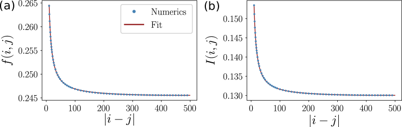
Figure 7: Finite-size scaling of correlation functions for the Heisenberg anti-ferromagnetic honeycomb model in the presence of a staggered magnetic field: (a) Function $f(\vec{r})=c_{0}+c_{1}r^{-\alpha}$ with coefficients $c_{0}=0.245$, $c_{1}=0.12$ and $\alpha=1.04$; (b) Valence bond correlation function $I(\vec{r})=c_{0}+c_{1}r^{-\alpha}$ with coefficients $c_{0}=0.13$, $c_{1}=0.155$ and $\alpha=1.07$. We set $h=1.23\times 10^{-11}$ and the total size $N=1000$.

F.3 Closed form of the valence bond correlator

Next, we study the response of valence bond correlation functions in the Néel state. We adopt the same definition as the Kitaev honeycomb model

$$I(i,j)=\langle Q_{i}Q_{j}\rangle-\langle Q_{i}\rangle\langle Q_{j}\rangle,\quad Q_{i}=S_{i_{1}}^{z}S_{i_{2}}^{z}.$$ (F14)

The bond index $\langle i_{1}i_{2}\rangle$ denotes two sites in the $i$-th unit cell of the sublattice $\{1\}$ and $\{2\}$. In the modified spin-wave theory, $S_{i_{1}}^{z}=1/2-a_{i}^{\dagger}a_{i}$, $S_{i,2}^{z}=-(1/2-b_{i}^{\dagger}b_{i})$. Reassembling different terms, we reach

$$16I(i,j)$$

$$=\sum_{k,l=1,2}\left<\hat{n}_{k}\hat{m}_{l}\right>+\left[2\left(\langle\hat{n}_{1}\hat{n}_{2}\rangle+\langle\hat{m}_{1}\hat{m}_{2}\rangle\right)-\left<\hat{n}_{1}\hat{n}_{2}\right>\left<\hat{m}_{1}\hat{m}_{2}\right>\right]$$

$$\phantom{=}-\sum_{k=1,2}\left[\left<\hat{n}_{k}\hat{m}_{1}\hat{m}_{2}\right>+\left<\hat{n}_{1}\hat{n}_{2}\hat{m}_{k}\right>\right]+\left<\hat{n}_{1}\hat{n}_{2}\hat{m}_{1}\hat{m}_{2}\right>-4.$$ (F15)

To simplify the notation, we have introduced a new set of number operators

$$\hat{n}_{1}=2a_{i}^{\dagger}a_{i},\quad\hat{n}_{2}=2b_{i}^{\dagger}b_{i},$$

$$\hat{m}_{1}=2a_{j}^{\dagger}a_{j},\quad\hat{m}_{2}=2b_{j}^{\dagger}b_{j}.$$ (F16)

First, taking into account $\langle a_{i}^{\dagger}a_{i}\rangle=\langle b_{i}^{\dagger}b_{i}\rangle=-{1}/{2}+f(\vec{0})={1}/{2}$, the single-particle expectation values become

$$\langle\hat{n}_{1}\rangle=\langle\hat{n}_{2}\rangle=\langle\hat{m}_{1}\rangle=\langle\hat{m}_{2}\rangle=1.$$ (F17)

.

Then, Wick’s theorem can be applied to calculate the remaining terms involving (2,3,4)-particle expectation values. Before proceeding, from Eq. (F3) we identify three useful functions

$$i\neq j,$$

$$f=f(|\vec{r}_{i}-\vec{r}_{j}|)=\langle a_{i}^{\dagger}a_{j}\rangle=\langle b_{i}^{\dagger}b_{j}\rangle=\langle a_{j}^{\dagger}a_{i}\rangle=\langle b_{j}^{\dagger}b_{i}\rangle;$$

$$g=g(|\vec{r}_{i}-\vec{r}_{j}|)=\langle a_{i}^{\dagger}b_{j}^{\dagger}\rangle=\langle a_{i}b_{j}\rangle=\langle a_{j}^{\dagger}b_{i}^{\dagger}\rangle=\langle a_{j}b_{i}\rangle;$$

$$i=j,$$

$$g_{0}=\langle a_{i}^{\dagger}b_{i}^{\dagger}\rangle=\langle a_{i}b_{i}\rangle=-0.692.$$ (F18)

All the other terms like $\langle a_{i}^{\dagger}a_{j}^{\dagger}\rangle$ and $\langle a_{i}^{\dagger}b_{j}\rangle$ vanish in the ground state. Two-particle expectation values then read

$$\langle\hat{n}_{1}\hat{m}_{1}\rangle =1+4f^{2}=\langle\hat{n}_{2}\hat{m}_{2}\rangle,$$

$$\langle\hat{n}_{1}\hat{m}_{2}\rangle =1+4g^{2}=\langle\hat{n}_{2}\hat{m}_{1}\rangle,$$

$$\langle\hat{n}_{1}\hat{n}_{2}\rangle =1+4g_{0}^{2}=\langle\hat{m}_{1}\hat{m}_{2}\rangle.$$ (F19)

The three-particle expectation value takes the form

$$\langle\hat{n}_{1}\hat{m}_{1}\hat{m}_{2}\rangle=1+4g_{0}^{2}+4(f^{2}+g^{2})+16g_{0}fg.$$ (F20)

The summation is invariant under the exchange of $(i\leftrightarrow j)$. Combined with the sublattice symmetries, we have

$$\langle\hat{n}_{1}\hat{m}_{1}\hat{m}_{2}\rangle=\langle\hat{n}_{1}\hat{n}_{2}\hat{m}_{1}\rangle=\langle\hat{n}_{1}\hat{n}_{2}\hat{m}_{2}\rangle=\langle\hat{n}_{2}\hat{m}_{1}\hat{m}_{2}\rangle.$$ (F21)

For the four-particle expectation value, we verify

$$\langle\hat{n}_{1}\hat{n}_{2}\hat{m}_{1}\hat{m}_{2}\rangle=\left[(1+4g_{0}^{2})+4(f^{2}+g^{2})\right]^{2}+64g_{0}fg.$$ (F22)

Therefore, we arrive at a closed form of the bond-bond correlators

$$I(i,j)=2g_{0}^{2}(f^{2}+g^{2})+(f^{2}+g^{2})^{2}.$$ (F23)

Considering the asymptotic behaviors of $f(\vec{r})$ and $g(\vec{r})$ functions in Eqs. (F12) and (F13), we establish

$$I(i,j)=c_{0}+\frac{c_{1}}{r}+\mathcal{O}(r^{-2}),$$ (F24)

where $c_{0}=4m_{0}^{2}(g_{0}^{2}+m_{0}^{2})\simeq 0.131$ and $c_{1}={m_{0}(3g_{0}^{2}+6m_{0}^{2})}/{\pi}\simeq 0.141$. Fig. 7 (b) confirms numerically the long-range behavior of the valence bond correlator with a power-law index $\alpha=1.07$. The two pre-factors $c_{0}=0.13,c_{1}=0.155$ are also consistent with our analytical predictions.

In the end, we find for the Néel state supported by strong antiferromagnetic Heisenberg exchanges, that the valence bond correlator gives a signature of the $r^{-1}$ scaling accompanied by a non-vanishing constant from finite-size effects (the regularization of the zero mode). This is clearly distinct from the pure $r^{-4}$ scaling in the gapless Kitaev spin liquid phase.

References

- Haldane [1983a] F. D. M. Haldane, Phys. Lett. A 93, 464 (1983a).
- Haldane [1983b] F. D. M. Haldane, Phys. Rev. Lett. 50, 1153 (1983b).
- Anderson [1987] P. W. Anderson, Science 235, 1196 (1987).
- Affleck et al. [1987] I. Affleck, T. Kennedy, E. H. Lieb, and H. Tasaki, Phys. Rev. Lett. 59, 799 (1987).
- Balents [2010] L. Balents, Nature 464, 199 (2010).
- Pollmann et al. [2012] F. Pollmann, E. Berg, A. M. Turner, and M. Oshikawa, Phys. Rev. B 85, 075125 (2012).
- Renard et al. [1988] J. Renard, M. Verdaguer, L. Regnault, W. Erkelens, J. Rossat-Mignod, J. Ribas, W. Stirling, and C. Vettier, J. Appl. Phys. 63, 3538 (1988).
- Alloul et al. [1989] H. Alloul, T. Ohno, and P. Mendels, Phys. Rev. Lett. 63, 1700 (1989).
- Johnston [1989] D. C. Johnston, Phys. Rev. Lett. 62, 957 (1989).
- Hagiwara et al. [1990] M. Hagiwara, K. Katsumata, I. Affleck, B. I. Halperin, and J. P. Renard, Phys. Rev. Lett. 65, 3181 (1990).
- Coldea et al. [2001] R. Coldea, D. Tennant, A. Tsvelik, and Z. Tylczynski, Phys. Rev. Lett. 86, 1335 (2001).
- Shimizu et al. [2003] Y. Shimizu, K. Miyagawa, K. Kanoda, M. Maesato, and G. Saito, Phys. Rev. Lett. 91, 107001 (2003).
- Mendels and Bert [2010] P. Mendels and F. Bert, J. Phys. Soc. Jpn. 79, 011001 (2010).
- Mendels and Bert [2016] P. Mendels and F. Bert, C. R. Phys. 17, 455 (2016).
- Takagi et al. [2019] H. Takagi, T. Takayama, G. Jackeli, G. Khaliullin, and S. E. Nagler, Nat. Rev. Phys. 1, 264 (2019).
- Kalmeyer and Laughlin [1987] V. Kalmeyer and R. B. Laughlin, Phys. Rev. Lett. 59, 2095 (1987).
- Kivelson et al. [1987] S. A. Kivelson, D. S. Rokhsar, and J. P. Sethna, Phys. Rev. B 35, 8865 (1987).
- Wen et al. [1989] X. G. Wen, F. Wilczek, and A. Zee, Phys. Rev. B 39, 11413 (1989).
- Read and Sachdev [1991] N. Read and S. Sachdev, Phys. Rev. Lett. 66, 1773 (1991).
- Kitaev and Laumann [2009] A. Kitaev and C. Laumann, arXiv:0904.2771 (2009).
- Kitaev [2006] A. Kitaev, Ann. Phys. 321, 2 (2006).
- Moore and Read [1991] G. Moore and N. Read, Nucl. Phys. B 360, 362 (1991).
- Read and Green [2000] N. Read and D. Green, Phys. Rev. B 61, 10267 (2000).
- Baskaran et al. [2007] G. Baskaran, S. Mandal, and R. Shankar, Phys. Rev. Lett. 98, 247201 (2007).
- Tikhonov et al. [2011] K. S. Tikhonov, M. V. Feigel’man, and A. Kitaev, Phys. Rev. Lett. 106, 067203 (2011).
- Knolle et al. [2014] J. Knolle, D. Kovrizhin, J. Chalker, and R. Moessner, Phys. Rev. Lett. 112, 207203 (2014).
- Song et al. [2016] X.-Y. Song, Y.-Z. You, and L. Balents, Phys. Rev. Lett. 117, 037209 (2016).
- Halász et al. [2018] G. B. Halász, S. Kourtis, J. Knolle, and N. B. Perkins, arXiv:1811.04951 (2018).
- Gohlke et al. [2018] M. Gohlke, R. Moessner, and F. Pollmann, Phys. Rev. B 98, 014418 (2018).
- Yao and Qi [2010] H. Yao and X.-L. Qi, Phys. Rev. Lett. 105, 080501 (2010).
- Eisert et al. [2010] J. Eisert, M. Cramer, and M. B. Plenio, Rev. Mod. Phys. 82, 277 (2010).
- Rau et al. [2016] J. G. Rau, E. K.-H. Lin, and H.-Y. Kee, Annu. Rev. Condens. Matter Phys. 7, 195 (2016).
- Trebst [2017] S. Trebst, arXiv:1701.07056 (2017).
- Kitagawa et al. [2018] K. Kitagawa, T. Takayama, Y. Matsumoto, A. Kato, R. Taken, Y. Kishimoto, S. Bette, G. Dinnebier, G. Jackeli, and H. Takagi, Nature 554, 341 (2018).
- Banerjee et al. [2017] A. Banerjee, J. Yan, J. Knolle, C. A. Bridges, M. B. Stone, M. D. Lumsden, D. G. Mandrus, D. A. Tennant, R. Moessner, and S. Nagler, Science 356, 1055 (2017).
- Nasu et al. [2016] J. Nasu, J. Knolle, D. Kovrizhin, Y. Motome, and R. Moessner, Nat. Phys. 12, 912 (2016).
- Janša et al. [2018] N. Janša, A. Zorko, M. Gomilšek, M. Pregelj, K. W. Krämer, D. Biner, A. Biffin, C. Rüegg, and M. Klanjšek, Nat. Phys. 14, 786 (2018).
- Nasu et al. [2017] J. Nasu, J. Yoshitake, and Y. Motome, Phys. Rev. Lett. 119, 127204 (2017).
- Kasahara et al. [2018a] Y. Kasahara, K. Sugii, T. Ohnishi, M. Shimozawa, M. Yamashita, N. Kurita, H. Tanaka, J. Nasu, Y. Motome, T. Shibauchi, and Y. Matsuda, Phys. Rev. Lett. 120, 217205 (2018a).
- Kasahara et al. [2018b] Y. Kasahara, T. Ohnishi, Y. Mizukami, O. Tanaka, S. Ma, K. Sugii, N. Kurita, H. Tanaka, J. Nasu, Y. Motome, et al., Nature 559, 227 (2018b).
- Duan et al. [2003] L.-M. Duan, E. Demler, and M. D. Lukin, Phys. Rev. Lett. 91, 090402 (2003).
- Yang et al. [2018] F. Yang, L. Henriet, A. Soret, and K. Le Hur, Phys. Rev. B 98, 035431 (2018).
- Sagi et al. [2018] E. Sagi, H. Ebisu, Y. Tanaka, A. Stern, and Y. Oreg, arXiv:1806.03304 (2018).
- Alet et al. [2007] F. Alet, S. Capponi, N. Laflorencie, and M. Mambrini, Phys. Rev. Lett. 99, 117204 (2007).
- Feng et al. [2007] X.-Y. Feng, G.-M. Zhang, and T. Xiang, Phys. Rev. Lett. 98, 087204 (2007).
- Le Hur et al. [2017] K. Le Hur, A. Soret, and F. Yang, Phys. Rev. B 96, 2015109 (2017).
- Yang et al. [2008] S. Yang, S.-J. Gu, C.-P. Sun, and H.-Q. Lin, Phys. Rev. A 78, 012304 (2008).
- Hickey and Trebst [2019] C. Hickey and S. Trebst, Nat. Commun. 10, 530 (2019).
- Song et al. [2012] H. F. Song, S. Rachel, C. Flindt, I. Klich, N. Laflorencie, and K. Le Hur, Phys. Rev. B 85, 035409 (2012).
- Petrescu et al. [2014] A. Petrescu, H. F. Song, S. Rachel, Z. Ristivojevic, C. Flindt, N. Laflorencie, I. Klich, N. Regnault, and K. Le Hur, J. Stat. Mech. 2014, P10005 (2014).
- Herviou et al. [2017] L. Herviou, C. Mora, and K. Le Hur, Phys. Rev. B 96, 121113 (2017).
- Kjäll et al. [2014] J. A. Kjäll, J. H. Bardarson, and F. Pollmann, Phys. Rev. Lett. 113, 107204 (2014).
- Ohya and Petz [2004] M. Ohya and D. Petz, Quantum entropy and its use (Springer Science & Business Media, 2004).
- Nishioka [2018] T. Nishioka, Rev. Mod. Phys. 90, 035007 (2018).
- Wolf et al. [2008] M. M. Wolf, F. Verstraete, M. B. Hastings, and J. I. Cirac, Phys. Rev. Lett. 100, 070502 (2008).
- Song et al. [2011] H. F. Song, N. Laflorencie, S. Rachel, and K. Le Hur, Phys. Rev. B 83, 224410 (2011).
- Rachel et al. [2012] S. Rachel, N. Laflorencie, H. F. Song, and K. Le Hur, Phys. Rev. Lett. 108, 116401 (2012).
- Yao and Lee [2011] H. Yao and D.-H. Lee, Phys. Rev. Lett. 107, 087205 (2011).
- Affleck and Ludwig [1991] I. Affleck and A. W. Ludwig, Phys. Rev. Lett. 67, 161 (1991).
- Alkurtass et al. [2016] B. Alkurtass, A. Bayat, I. Affleck, S. Bose, H. Johannesson, P. Sodano, E. S. Sørensen, and K. Le Hur, Phys. Rev. B 93, 081106 (2016).
- Song et al. [2010] H. F. Song, S. Rachel, and K. Le Hur, Phys. Rev. B 82, 012405 (2010).
- Calabrese and Cardy [2004] P. Calabrese and J. Cardy, J. Stat. Mech. 2004, P06002 (2004).
- Lieb [1994] E. H. Lieb, Phys. Rev. Lett. 73, 2158 (1994).
- Herviou et al. [2019] L. Herviou, K. Le Hur, and C. Mora, Phys. Rev. B 99, 075133 (2019).
- Peschel [2003] I. Peschel, J. Phys. A 36, L205 (2003).
- Takahashi [1989] M. Takahashi, Phys. Rev. B 40, 2494 (1989).
- Hermanns and Trebst [2014] M. Hermanns and S. Trebst, Phys. Rev. B 89, 235102 (2014).
- Hermanns et al. [2017] M. Hermanns, I. Kimchi, and J. Knolle, Annu. Rev. Condens. Matter Phys. 9, 17 (2017).