Regge pole description of scattering of scalar and electromagnetic waves
by a Schwarzschild black hole

Abstract

We revisit the problem of scalar and electromagnetic waves impinging upon a Schwarzschild black hole from complex angular momentum techniques. We focus more particularly on the associated differential scattering cross sections. We derive an exact representation of the corresponding scattering amplitudes by replacing the discrete sum over integer values of the angular momentum which defines their partial wave expansions by a background integral in the complex angular momentum plane plus a sum over the Regge poles of the $S$-matrix involving the associated residues. We show that, surprisingly, the background integral is numerically negligible for intermediate and high frequencies and, as a consequence, that the cross sections can be reconstructed in terms of Regge poles with very good agreement. We show in particular that, for large values of the scattering angle, a small number of Regge poles permits us to describe the black hole glory and that, by increasing the number of Regge poles, we can reconstruct very efficiently the differential scattering cross sections for small and intermediate scattering angles and therefore describe the orbiting oscillations. In fact, in the short-wavelength regime, the sum over Regge poles allows us to extract by resummation the information encoded in the partial wave expansion defining a scattering amplitude and, moreover, to overcome the difficulties linked to its lack of convergence due to the long-range nature of the fields propagating on the black hole. As a consequence, from asymptotic expressions for the lowest Regge poles and the associated residues based on the correspondence Regge poles – “surface waves” propagating close to the photon sphere, we can provide an analytical approximation describing both the black hole glory and a large part of the orbiting oscillations. We finally discuss the role of the background integral for low frequencies.

I Introduction

Studies concerning the scattering of waves by black holes (BHs) are mainly based on partial wave expansions (see, e.g., Ref. Futterman et al. (2012)). This is due to the high degree of symmetry of the BH spacetimes usually considered and physically or astrophysically interesting. For example, the Schwarzschild BH is a static spherically symmetric solution of the vacuum Einstein’s equations while the Kerr BH is a stationary axisymmetric solution of these equations with, as a consequence, the separability of wave equations on these gravitational backgrounds (see, e.g., Ref. Frolov and Novikov (1998)). Even if the approach based on partial wave expansions is natural and very effective in the context of scattering of waves by BHs, it presents some flaws. Due to the long-range nature of the fields propagating on a BH, some partial wave expansions encountered are formally divergent (see, e.g., Ref. Futterman et al. (2012)) and, moreover, it is in general rather difficult to interpret physically results described in terms of partial wave expansions. These problems can be overcome by using complex angular momentum (CAM) techniques (analytic continuation of partial wave expansions in the CAM plane, effective resummations involving the poles of the $S$-matrix in the CAM plane, i.e., the so-called Regge poles, and the associated residues, semiclassical interpretations of Regge pole expansions, etc.). Such techniques, which proved to be very helpful in quantum mechanics (see, e.g., Refs. de Alfaro and Regge (1965); Newton (1982)), in electromagnetism and optics (see, e.g., Refs. Watson (1918); Sommerfeld (1949); Newton (1982); Nussenzveig (1992); Grandy (2000)), in acoustics and seismology (see, e.g., Refs. Überall (1992); Aki and Richards (2002)) and in high-energy physics (see, e.g., Refs. Gribov (2003); Collins (1977); Barone and Predazzi (2002); Donnachie et al. (2005)) to describe and analyze resonant scattering are now also used in the context of BH physics (see, e.g., Refs. Andersson and Thylwe (1994); Andersson (1994); Decanini et al. (2003); Glampedakis and Andersson (2003); Decanini and Folacci (2010, 2009); Dolan and Ottewill (2009); Decanini et al. (2010, 2011a, 2011b, 2011c); Dolan et al. (2012); Macedo et al. (2013); Nambu and Noda (2016); Folacci and Ould El Hadj (2018); Benone et al. (2018)).

In this article we revisit the problem of plane monochromatic waves impinging upon a Schwarzschild BH from CAM techniques. More precisely, we focus on the differential scattering cross sections associated with scalar and electromagnetic waves. It should be recalled that the partial wave expansions of these cross sections have been obtained a long time ago by Matzner Matzner (1968) for the scalar field and by Mashhoon Mashhoon (1973, 1974) and Fabbri Fabbri (1975) for the electromagnetic field and that many additional works have since been done which have theoretically and numerically completed these first investigations (see, e.g., Refs. Sanchez (1976, 1978); Matzner et al. (1985); Anninos et al. (1992); Andersson and Thylwe (1994); Andersson (1994, 1995); Glampedakis and Andersson (2001); Dolan (2008a); Crispino et al. (2009a) for some articles directly relevant to our own study). It is furthermore worth noting that the important case of the electromagnetic field is of fundamental interest with the emergence of multimessenger astronomy as well as with the possibility to produce experimentally BH images or, more precisely, to “photograph” with the Event Horizon Telescope the shadow of supermassive BHs Falcke et al. (2000); Castelvecchi (2017); Collaboration (2019). Here, we construct an exact representation of the scalar and electromagnetic scattering cross sections by replacing the discrete sum over integer values of the angular momentum which defines their partial wave expansions by a background integral in the CAM plane plus a sum over the Regge poles of the $S$-matrix which involves the associated residues. Surprisingly, we find that the background integral is numerically negligible for intermediate and high reduced frequencies (i.e., in the short-wavelength regime) and, as a consequence, that the differential scattering cross sections can be described in terms of Regge poles with very good agreement for arbitrary scattering angles. In fact, in this wavelength regime, the sum over Regge poles allows us to extract by resummation the physical information encoded in the partial wave expansion defining a differential scattering cross section and, moreover, to overcome the difficulties linked to its lack of convergence due to the long-range nature of the fields propagating on the BH. We show in particular that, for large values of the scattering angle, i.e., in the backward direction, a small number of Regge poles permits us to describe the BH glory (see Refs. Matzner et al. (1985); Andersson (1994) for semiclassical interpretations) and that, by increasing the number of Regge poles, we can reconstruct very efficiently the differential scattering cross sections for small and intermediate scattering angles and therefore describe the orbiting oscillations (see Refs. Anninos et al. (1992); Andersson (1994) for semiclassical interpretations). We then take advantage of these numerical results to derive an analytical approximation fitting both the BH glory and a large part of the orbiting oscillations. This is achieved by inserting in the Regge pole sums asymptotic approximations for the lowest Regge poles and the associated residues.

It is important to relate or compare our results with other results previously obtained:

1. Our work extends but also corrects the important studies by Andersson and Thylwe Andersson and Thylwe (1994); Andersson (1994) where we can find the first application of CAM techniques in BH physics. In Ref. Andersson and Thylwe (1994), Andersson and Thylwe have considered the scattering of scalar waves by a Schwarzschild BH from a theoretical point of view and adapted the CAM formalism to this problem. They have established some properties of the Regge poles and of the $S$-matrix in the CAM plane. In Ref. Andersson (1994), Andersson has used this formalism to interpret semiclassically the BH glory and the orbiting oscillations. He has, in particular, considered “surface waves” propagating close to the unstable circular photon (graviton) orbit at $r=3M$, i.e., near the so-called photon sphere, and associated them with the Regge poles. However, it should be noted that some of the analyses and comments we can find in Ref. Andersson (1994) are invalidated by the fact that the residues numerically obtained are incorrect (see also Ref. Glampedakis and Andersson (2003)). In our article, we obtain precise values for the residues of a large number of Regge poles, thus permitting us to draw solid conclusions from our results. Furthermore, we show that the background integral in the CAM plane is numerically negligible for intermediate and high reduced frequencies. Here, it is important to recall that, in Refs. Andersson and Thylwe (1994); Andersson (1994), Andersson and Thylwe tried to extract some physical information of this background integral and that, in electromagnetism and optics Watson (1918); Sommerfeld (1949); Newton (1982); Nussenzveig (1992); Grandy (2000) as well as in acoustics and seismology Überall (1992); Aki and Richards (2002)), it can be associated semiclassically (i.e., for high reduced frequencies) with incident and reflected rays. In the context of scattering by BHs (or, more precisely, if we focus on differential scattering cross sections in the short-wavelength regime), it plays only a minor role.

2. We have developed Andersson’s point of view concerning the surface waves propagating close to the photon sphere in a series of papers establishing, in particular, that the complex frequencies of the weakly damped quasinormal modes (QNMs) are Breit-Wigner-type resonances generated by these surface waves. We have then been able to construct semiclassically the spectrum of the QNM complex frequencies from the Regge trajectories, i.e., from the curves traced out in the CAM plane by the Regge poles as a function of the frequency Decanini et al. (2003); Decanini and Folacci (2010); Folacci and Ould El Hadj (2018), establishing on a “rigorous” basis the physically intuitive interpretation of the Schwarzschild BH QNMs suggested, as early as 1972, by Goebel Goebel (1972) (see Refs. Decanini and Folacci (2009); Dolan and Ottewill (2009); Decanini et al. (2010, 2011a) for the extension of these results to other BHs and to massive fields). Moreover, from the Regge trajectories and the residues of the greybody factors, we have described analytically the high-energy absorption cross section for a wide class of BHs endowed with a photon sphere and explained its oscillations in terms of the geometrical characteristics (orbital period and Lyapunov exponent) of the null unstable geodesics lying on the photon sphere Decanini et al. (2011b, c, a). All these results highlight the interpretive power of CAM techniques in BH physics.

3. In order to derive analytical approximations which fit both the BH glory and a large part of the orbiting oscillations, we shall insert into the Regge pole sums asymptotic expansions for the Regge poles and the associated residues. In fact, such expansions which are valid in the short-wavelength regime are physically connected with the excitation of the surface waves previously mentioned and with diffractive effects due to the Schwarzschild photon sphere Andersson (1994); Decanini et al. (2003); Decanini and Folacci (2010); Dolan and Ottewill (2009); Decanini et al. (2010, ). It is moreover important to recall that glory scattering and orbiting scattering are usually considered as two different effects and are described analytically by two different semiclassical analytic formulas (see Refs. Matzner et al. (1985); Anninos et al. (1992) or Sec. 4.7.2 of Ref. Frolov and Novikov (1998) for a concise presentation). Here, we prove that it is possible from Regge pole sums to describe analytically both phenomena in a unique formula.

Our paper is organized as follows. In Sec. II, by means of the Sommerfeld-Watson transform Watson (1918); Sommerfeld (1949); Newton (1982) and Cauchy’s residue theorem, we construct exact CAM representations of the differential scattering cross sections for plane scalar and electromagnetic waves impinging upon a Schwarzschild BH from their partial wave expansions. These CAM representations are split into a background integral in the CAM plane and a sum over the Regge poles of the $S$-matrix involving the associated residues. In Sec. III, we obtain numerically, for various reduced frequencies, the Regge poles of the $S$-matrix, the associated residues and the background integral. This permits us to reconstruct, for these particular frequencies of the impinging waves, the differential scattering cross sections of the BH and to show that, in the short-wavelength regime, they can be described from the Regge pole sum alone with very good agreement. We also discuss the role of the background integral for low reduced frequencies, i.e., in the long-wavelength regime. In Sec. IV, by inserting into the Regge pole sum asymptotic approximations for the lowest Regge poles and the associated residues, we derive a formula fitting both the BH glory and a large part of the orbiting oscillations. In the Conclusion, we summarize our main results and briefly consider possible extensions of our work. In the Appendix, we discuss the numerical evaluation of the background integrals. Due to the long-range nature of the fields propagating on a Schwarzschild BH, these integrals in the CAM plane (as the partial wave expansions) suffer a lack of convergence. We overcome this problem, i.e., we accelerate their convergence, by extending to integrals the iterative method developed in Ref. Yennie et al. (1954) for partial wave expansions.

Throughout this article, we adopt units such that $G=c=1$. We furthermore consider that the exterior of the Schwarzschild BH is defined by the line element $ds^{2}=-f(r)dt^{2}+f(r)^{-1}dr^{2}+r^{2}d\theta^{2}+r^{2}\sin^{2}\theta d\varphi^{2}$ where $f(r)=1-2M/r$ and $M$ is the mass of the BH while $t\in]-\infty,+\infty[$, $r\in]2M,+\infty[$, $\theta\in[0,\pi]$ and $\varphi\in[0,2\pi]$ are the usual Schwarzschild coordinates. We finally assume a time dependence $\exp(-i\omega t)$ for the plane monochromatic waves considered.

II Differential scattering cross sections for scalar and electromagnetic waves, their CAM representations and their Regge pole approximations

In this section, we recall the partial wave expansions of the differential scattering cross sections for plane monochromatic scalar and electromagnetic waves impinging upon a Schwarzschild BH and we construct exact CAM representations of these cross sections by means of the Sommerfeld-Watson transform Watson (1918); Sommerfeld (1949); Newton (1982) and Cauchy’s theorem. These CAM representations are split into a background integral in the CAM plane and a sum over the Regge poles of the $S$-matrix involving the associated residues.

II.1 Partial wave expansions of differential scattering cross sections

We recall that, for the scalar field, the differential scattering cross section is given by Matzner (1968)

$$\frac{d\sigma}{d\Omega}=|f(\omega,\theta)|^{2}$$ (1)

where

$$f(\omega,\theta)=\frac{1}{2i\omega}\sum_{\ell=0}^{\infty}(2\ell+1)[S_{\ell}(\omega)-1]P_{\ell}(\cos\theta)$$ (2)

denotes the scattering amplitude and that, for the electromagnetic field, the differential scattering cross section can be written in the form Mashhoon (1973, 1974) (see also Refs. Fabbri (1975); Crispino et al. (2009a))

$$\frac{d\sigma}{d\Omega}=|A(\omega,\theta)|^{2}$$ (3)

where the scattering amplitude is given by

$$A(\omega,\theta)=\mathcal{D}_{\theta}B(\omega,\theta)$$ (4)

with

$$B(\omega,\theta)=\frac{1}{2i\omega}\sum_{\ell=1}^{\infty}\frac{(2\ell+1)}{\ell(\ell+1)}[S_{\ell}(\omega)-1]P_{\ell}(\cos\theta)$$ (5)

and

$$\mathcal{D}_{\theta} = -(1+\cos\theta)\frac{d\,\,\,}{d\cos\theta}\left[(1-\cos\theta)\frac{d\,\,\,}{d\cos\theta}\right]$$ (6a)

$$= -\left(\frac{d^{2}}{d\theta^{2}}+\frac{1}{\sin\theta}\frac{d}{d\theta}\right).$$ (6b)

The expression (4)-(6) takes into account the two polarizations of the electromagnetic field. In Eqs. (2) and (5), the functions $P_{\ell}(\cos\theta)$ are the Legendre polynomials Abramowitz and Stegun (1965). We also recall that the $S$-matrix elements $S_{\ell}(\omega)$ appearing in Eqs. (2) and (5) can be defined from the modes $\phi_{\omega\ell}^{in}$ solutions of the homogenous Regge-Wheeler equation

$$\left[\frac{d^{2}}{dr_{\ast}^{2}}+\omega^{2}-V_{\ell}(r)\right]\phi_{\omega\ell}=0$$ (7)

[here $r^{\ast}=r+2M\ln[r/(2M)-1]+\mathrm{const}$ denotes the tortoise coordinate] where

$$V_{\ell}(r)=\left(1-\frac{2M}{r}\right)\left(\frac{\ell(\ell+1)}{r^{2}}+(1-s^{2})\frac{2M}{r^{3}}\right)$$ (8)

(here $s=0$ corresponds to the scalar field and $s=1$ to the electromagnetic field) which have a purely ingoing behavior at the event horizon $r=2M$ (i.e., for $r_{\ast}\to-\infty$)

$$\phi^{\mathrm{in}}_{\omega\ell}(r)\scriptstyle{\underset{r_{\ast}\to-\infty}{\sim}}\displaystyle{e^{-i\omega r_{\ast}}}$$ (9a)

and, at spatial infinity $$r\to+\infty r_{\ast}\to+\infty$$ (i.e., for ), an asymptotic behavior of the form

$$\phi^{\mathrm{in}}_{\omega\ell}(r)\scriptstyle{\underset{r_{\ast}\to+\infty}{\sim}}\displaystyle{A^{(-)}_{\ell}(\omega)e^{-i\omega r_{\ast}}+A^{(+)}_{\ell}(\omega)e^{+i\omega r_{\ast}}}.$$ (9b)

In this last equation, the coefficients $A^{(-)}_{\ell}(\omega)$ and $A^{(+)}_{\ell}(\omega)$ are complex amplitudes and we have

$$S_{\ell}(\omega)=e^{i(\ell+1)\pi}\,\frac{A_{\ell}^{(+)}(\omega)}{A_{\ell}^{(-)}(\omega)}.$$ (10)

II.2 CAM representation of the scattering amplitude for scalar waves

II.2.1 Sommerfeld-Watson representation of the scattering amplitude

By means of the Sommerfeld-Watson transformation Watson (1918); Sommerfeld (1949); Newton (1982) which permits us to write

$$\sum_{\ell=0}^{+\infty}(-1)^{\ell}F(\ell)=\frac{i}{2}\int_{\cal C}d\lambda\,\frac{F(\lambda-1/2)}{\cos(\pi\lambda)}$$ (11)

for a function $F$ without any singularities on the real $\lambda$ axis, we can replace in Eq. (2) the discrete sum over the ordinary angular momentum $\ell$ by a contour integral in the complex $\lambda$ plane (i.e., in the complex $\ell$ plane with $\lambda=\ell+1/2$). By noting that $P_{\ell}(\cos\theta)=(-1)^{\ell}P_{\ell}(-\cos\theta)$, we obtain

$$f(\omega,\theta)=\frac{1}{2\omega}\int_{\cal C}d\lambda\,\frac{\lambda}{\cos(\pi\lambda)}$$

$$\qquad\qquad\times\left[S_{\lambda-1/2}(\omega)-1\right]P_{\lambda-1/2}(-\cos\theta).$$ (12)

In Eqs. (11) and (II.2.1), the integration contour encircles counterclockwise the positive real axis of the complex $\lambda$ plane, i.e., we take ${\cal C}=]+\infty+i\epsilon,+i\epsilon]\cup[+i\epsilon,-i\epsilon]\cup[-i\epsilon,+\infty-i\epsilon[$ with $\epsilon\to 0_{+}$ (see Fig. 1). We can recover (2) from (II.2.1) by using Cauchy’s theorem and by noting that the poles of the integrand in (II.2.1) that are enclosed into ${\cal C}$ are the zeros of $\cos(\pi\lambda)$, i.e., the semi-integers $\lambda=\ell+1/2$ with $\ell\in\mathbb{N}$. It should be recalled that, in Eq. (II.2.1), the Legendre function of first kind $P_{\lambda-1/2}(z)$ denotes the analytic extension of the Legendre polynomials $P_{\ell}(z)$. It is defined in terms of hypergeometric functions by Abramowitz and Stegun (1965)

$$P_{\lambda-1/2}(z)=F[1/2-\lambda,1/2+\lambda;1;(1-z)/2].$$ (13)

In Eq. (II.2.1), $S_{\lambda-1/2}(\omega)$ denotes “the” analytic extension of $S_{\ell}(\omega)$. It is given by [see Eq. (10)]

$$S_{\lambda-1/2}(\omega)=e^{i(\lambda+1/2)\pi}\,\frac{A_{\lambda-1/2}^{(+)}(\omega)}{A_{\lambda-1/2}^{(-)}(\omega)}$$ (14)

where the complex amplitudes $A^{(-)}_{\lambda-1/2}(\omega)$ and $A^{(+)}_{\lambda-1/2}(\omega)$ are defined from the analytic extension of the modes $\phi_{\omega\ell}^{in}$, i.e., from the function $\phi_{\omega,\lambda-1/2}^{in}$ solution of the problem (7)-(9) where we now replace $\ell$ by $\lambda-1/2$. With the deformation of the contour ${\cal C}$ in mind, it is important to note the symmetry property

$$e^{i\pi\lambda}\,S_{-\lambda-1/2}(\omega)=e^{-i\pi\lambda}\,S_{\lambda-1/2}(\omega)$$ (15)

of the $S$-matrix which can be easily obtained from its definition (see also Ref. Andersson and Thylwe (1994)).

Figure 1: The integration contour ${\cal C}={\cal C}_{+}\,\cup\,{\cal C}_{-}$ in the complex $\lambda$ plane. It defines the scattering amplitude (II.2.1) and its deformations permit us to collect, by using Cauchy’s theorem, the contributions of the Regge poles $\lambda_{n}(\omega)$.

II.2.2 Regge poles and associated residues

With the deformation of the contour ${\cal C}$ in mind, it is also important to recall that the poles of $S_{\lambda-1/2}(\omega)$ in the complex $\lambda$ plane (i.e., the Regge poles) lie in the first and third quadrants of this plane, symmetrically distributed with respect to the origin $O$. The poles lying in the first quadrant can be defined as the zeros $\lambda_{n}(\omega)$ with $n=1,2,3,\dots$ of the coefficient $A^{(-)}_{\lambda-1/2}(\omega)$ [see Eq. (14)]. They therefore satisfy

$$A^{(-)}_{\lambda_{n}(\omega)-1/2}(\omega)=0.$$ (16)

In the following, the associated residues will play a central role. We note that the residue of the matrix $S_{\lambda-1/2}(\omega)$ at the pole $\lambda=\lambda_{n}(\omega)$ is defined by [see Eq. (14)]

$$r_{n}(\omega)=e^{i\pi[\lambda_{n}(\omega)+1/2]}\left[\frac{A_{\lambda-1/2}^{(+)}(\omega)}{\frac{d}{d\lambda}A_{\lambda-1/2}^{(-)}(\omega)}\right]_{\lambda=\lambda_{n}(\omega)}.$$ (17)

II.2.3 CAM representation of the scattering amplitude

We can now “deform” the contour ${\cal C}$ in Eq. (II.2.1) in order to collect, by using Cauchy’s theorem, the contributions of the Regge poles lying in the first quadrant of the CAM plane (for more details, see, e.g., Ref. Newton (1982)). We consider that ${\cal C}={\cal C}_{+}\cup{\cal C}_{-}$ with ${\cal C}_{+}=]+\infty+i\epsilon,+i\epsilon]\cup[+i\epsilon,0]$ and ${\cal C}_{-}=[0,-i\epsilon]\cup[-i\epsilon,+\infty-i\epsilon[$ and we introduce the closed contours ${\cal C}_{+}\,\cup\,[0,+i\infty[\,\cup\,{\cal C}_{\infty+}$ and ${\cal C}_{-}\,\cup\,{\cal C}_{\infty-}\,\cup\,[-i\infty,0]$ (see Fig. 1). Here, the integration paths ${\cal C}_{\infty+}$ and ${\cal C}_{\infty-}$ are quarter circles at infinity lying respectively in the first and fourth quadrants of the complex $\lambda$ plane.

We first use Cauchy’s residue theorem in connection with the closed contour ${\cal C}_{+}\,\cup\,[0,+i\infty[\,\cup\,{\cal C}_{\infty+}$. We obtain

$$\int_{{\cal C}_{+}}d\lambda\,\frac{\lambda}{\cos(\pi\lambda)}\left[S_{\lambda-1/2}(\omega)-1\right]P_{\lambda-1/2}(-\cos\theta)$$

$$\quad=-\int_{0}^{+i\infty}d\lambda\,\frac{\lambda}{\cos(\pi\lambda)}\left[S_{\lambda-1/2}(\omega)-1\right]P_{\lambda-1/2}(-\cos\theta)$$

$$\quad\phantom{=}-2i\pi\sum_{n=1}^{+\infty}\frac{\lambda_{n}(\omega)r_{n}(\omega)}{\cos[\pi\lambda_{n}(\omega)]}P_{\lambda_{n}(\omega)-1/2}(-\cos\theta).$$ (18)

Here we have dropped the contribution coming from ${\cal C}_{\infty+}$ by noting that

$$\frac{\lambda}{\cos(\pi\lambda)}\left[S_{\lambda-1/2}(\omega)-1\right]P_{\lambda-1/2}(-\cos\theta)$$ (19)

vanishes faster than $1/\lambda$ for $|\lambda|\to+\infty$ and $\operatorname{Im}\lambda>0$.

We then use Cauchy’s residue theorem in connection with the closed contour ${\cal C}_{-}\,\cup\,{\cal C}_{\infty-}\,\cup\,]-i\infty,0]$. This must be done with great caution because

$$\frac{\lambda}{\cos(\pi\lambda)}S_{\lambda-1/2}(\omega)P_{\lambda-1/2}(-\cos\theta)$$ (20)

diverges for $|\lambda|\to+\infty$ and $\operatorname{Im}\lambda<0$ and, as a consequence, taking into account the contribution coming from the quarter circle ${\cal C}_{\infty-}$ is problematic. (It is interesting to note that, in addition, this result forbids us to collect, in a simple way, the Regge poles lying in the third quadrant of the complex $\lambda$ plane.) The difficulties encountered can be partially bypassed by using the relation Abramowitz and Stegun (1965)

$$Q_{\lambda-1/2}(\cos\theta+i0)=\frac{\pi}{2\cos(\pi\lambda)}\left[P_{\lambda-1/2}(-\cos\theta)\phantom{e^{-i\pi\lambda}}\right.$$

$$\qquad\qquad\left.-e^{-i\pi(\lambda-1/2)}P_{\lambda-1/2}(+\cos\theta)\right]$$ (21)

where $Q_{\lambda-1/2}(z)$ denotes the Legendre function of the second kind. Indeed, it permits us to replace (20) by the equivalent expression

$$\frac{\lambda}{\cos(\pi\lambda)}S_{\lambda-1/2}(\omega)e^{-i\pi(\lambda-1/2)}P_{\lambda-1/2}(+\cos\theta)$$

$$\qquad+\frac{2}{\pi}\lambda S_{\lambda-1/2}(\omega)Q_{\lambda-1/2}(\cos\theta+i0)$$ (22)

where the first term vanishes faster than $1/\lambda$ for $|\lambda|\to+\infty$ and $\operatorname{Im}\lambda<0$. By moreover noting that

$$\frac{\lambda}{\cos(\pi\lambda)}P_{\lambda-1/2}(-\cos\theta)$$ (23)

vanishes faster than $1/\lambda$ for $|\lambda|\to+\infty$ and $\operatorname{Im}\lambda<0$, we can write

$$\int_{{\cal C}_{-}}d\lambda\,\frac{\lambda}{\cos(\pi\lambda)}\left[S_{\lambda-1/2}(\omega)-1\right]P_{\lambda-1/2}(-\cos\theta)$$

$$\quad=\int_{-i\infty}^{0}d\lambda\,\frac{\lambda}{\cos(\pi\lambda)}P_{\lambda-1/2}(-\cos\theta)$$

$$\quad\phantom{=}+\frac{2}{\pi}\int_{{\cal C}_{-}}d\lambda\,\lambda S_{\lambda-1/2}(\omega)Q_{\lambda-1/2}(\cos\theta+i0)$$

$$\quad\phantom{=}-\int_{-i\infty}^{0}d\lambda\,\frac{\lambda}{\cos(\pi\lambda)}S_{\lambda-1/2}(\omega)$$

$$\qquad\qquad\qquad\qquad\times e^{-i\pi(\lambda-1/2)}P_{\lambda-1/2}(+\cos\theta).$$ (24)

We finally insert the results (II.2.3) and (II.2.3) into (II.2.1) and by using (15) as well as the relation Abramowitz and Stegun (1965)

$$P_{-\lambda-1/2}(z)=P_{\lambda-1/2}(z)$$ (25)

we obtain

$$f(\omega,\theta)=f^{\text{\tiny{B}}}(\omega,\theta)+f^{\text{\tiny{RP}}}(\omega,\theta)$$ (26)

where

$$f^{\text{\tiny{B}}}(\omega,\theta)=f^{\text{\tiny{B},\tiny{Re}}}(\omega,\theta)+f^{\text{\tiny{B},\tiny{Im}}}(\omega,\theta)$$ (27a)

with

$$f^{\text{\tiny{B},\tiny{Re}}}(\omega,\theta)=\frac{1}{\pi\omega}\int_{{\cal C}_{-}}d\lambda\,\lambda S_{\lambda-1/2}(\omega)Q_{\lambda-1/2}(\cos\theta+i0)$$ (27b)

and

$$f^{\text{\tiny{B},\tiny{Im}}}(\omega,\theta)=\frac{1}{\pi\omega}\int_{+i\infty}^{0}d\lambda\,\lambda S_{\lambda-1/2}(\omega)Q_{\lambda-1/2}(\cos\theta+i0)$$ (27c)

is a background integral contribution and where

$$f^{\text{\tiny{RP}}}(\omega,\theta)=-\frac{i\pi}{\omega}\sum_{n=1}^{+\infty}\frac{\lambda_{n}(\omega)r_{n}(\omega)}{\cos[\pi\lambda_{n}(\omega)]}$$

$$\qquad\qquad\qquad\qquad\times P_{\lambda_{n}(\omega)-1/2}(-\cos\theta)$$ (28)

is a sum over the Regge poles lying in the first quadrant of the CAM plane. Of course, Eqs. (26), (27) and (II.2.3) provide an exact representation of the scattering amplitude $f(\omega,\theta)$ for the scalar field, equivalent to the initial partial wave expansion (2). From this CAM representation, we can extract the contribution $f^{\text{\tiny{RP}}}(\omega,\theta)$ given by (II.2.3) which, as a sum over Regge poles, is only an approximation of $f(\omega,\theta)$, and which provides us with an approximation of the differential scattering cross section (1).

II.2.4 Remarks concerning the background integral

It is important to note that the path of integration defining the background integral (27) is a continuous one running down first the positive imaginary axis and then running along ${\cal C}_{-}$, i.e., slightly below the positive real axis. But, in fact, because the integrand in the right-hand side of (27b) is regular, this second branch can be deformed in order to coincide exactly with the positive real axis. As a consequence, we can take for the path of integration defining the background integral (27) the path $]+i\infty,0]\,\cup\,[0,+\infty[$ (see Fig. 3) and we can replace (27b) by

$$f^{\text{\tiny{B},\tiny{Re}}}(\omega,\theta)=\frac{1}{\pi\omega}\int_{0}^{+\infty}d\lambda\,\lambda S_{\lambda-1/2}(\omega)$$

$$\qquad\qquad\qquad\qquad\qquad\times Q_{\lambda-1/2}(\cos\theta+i0).$$ (29)

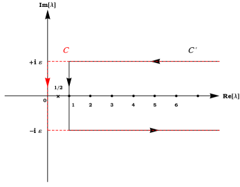
Figure 2: Integration contours in the CAM plane: ${\cal C^{\prime}}$ is associated with the scattering amplitude (32) and ${\cal C}$ with the scattering amplitude (II.3.1).

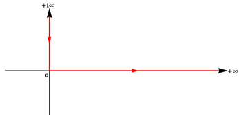
Figure 3: The path of integration in the complex $\lambda$ plane which defines the background integrals (27) and (39).

Moreover, with numerical calculations in mind, it is interesting to remark that the function $Q_{\lambda-1/2}(\cos\theta+i0)$ appearing in the integrand of the background integral can be expressed in the alternative forms Abramowitz and Stegun (1965)

$$Q_{\lambda-1/2}(\cos\theta+i0)=Q_{\lambda-1/2}(\cos\theta)$$ (30a)

$$\qquad\qquad\qquad\qquad\qquad-i\frac{\pi}{2}P_{\lambda-1/2}(\cos\theta)$$

and

$$Q_{\lambda-1/2}(\cos\theta+i0)=\frac{\Gamma(\lambda+1/2)}{\Gamma(\lambda+1)}\sqrt{\frac{\pi}{2\sin\theta}}e^{-i\left[\lambda\theta+\pi/4\right]}$$

$$\qquad\qquad\qquad\times F[1/2,1/2;\lambda+1;ie^{-i\theta}/(2\sin\theta)].$$ (30b)

II.3 CAM representation of the scattering amplitude for electromagnetic waves

II.3.1 Sommerfeld-Watson representation of the scattering amplitude

In order to obtain the CAM representation of the scattering amplitudes (4) and (5), we use the Sommerfeld-Watson transformation in the form

$$\sum_{\ell=1}^{+\infty}(-1)^{\ell}F(\ell)=\frac{i}{2}\int_{\cal C^{\prime}}d\lambda\,\frac{F(\lambda-1/2)}{\cos(\pi\lambda)}.$$ (31)

Here ${\cal C^{\prime}}=]+\infty+i\epsilon,1+i\epsilon]\cup[1+i\epsilon,1-i\epsilon]\cup[1-i\epsilon,+\infty-i\epsilon[$ with $\epsilon\to 0_{+}$ because we must take into account that the sum over $\ell$ defining the scattering amplitude (5) begins at $\ell=1$. We then obtain

$$B(\omega,\theta)=\frac{1}{2\omega}\int_{\cal C^{\prime}}d\lambda\,\frac{\lambda}{(\lambda^{2}-1/4)\cos(\pi\lambda)}$$ (32)

$$\qquad\qquad\times\left[S_{\lambda-1/2}(\omega)-1\right]P_{\lambda-1/2}(-\cos\theta).$$

With the collect of Regge poles in mind, the contour ${\cal C^{\prime}}$ is not as convenient as the contour ${\cal C}$ used in Sec. II.2. However, it is possible to move ${\cal C^{\prime}}$ to the left so that it coincides with ${\cal C}$ but we then introduce a spurious double pole at $\lambda=1/2$ (i.e., at $\ell=0$) corresponding to the term $1/[(\lambda-1/2)\cos(\pi\lambda)]$ (see Fig. 2). It is necessary to remove the associated residue contribution and we obtain

$$B(\omega,\theta)=\frac{1}{2\omega}\left(\int_{\cal C}d\lambda\,\frac{\lambda}{(\lambda^{2}-1/4)\cos(\pi\lambda)}\left[S_{\lambda-1/2}(\omega)-1\right]P_{\lambda-1/2}(-\cos\theta)\right.$$

$$\qquad\left.-2i\pi\lim_{\lambda\to 1/2}\frac{d}{d\lambda}\left[(\lambda-1/2)^{2}\times\frac{\lambda}{(\lambda^{2}-1/4)\cos(\pi\lambda)}\left[S_{\lambda-1/2}(\omega)-1\right]P_{\lambda-1/2}(-\cos\theta)\right]\right).$$ (33)

In this equation, the residue contribution can be explicitly derived by using

$$\left[\frac{d}{d\lambda}P_{\lambda-1/2}(-x)\right]_{\lambda=1/2}=\ln\left(\frac{1-x}{2}\right)$$ (34)

which is a consequence of the definition (13) and by noting that, for the electromagnetic field, we have formally $S_{0}(\omega)=0$ [see Eqs. (7)–(9)]. We can then write

$$B(\omega,\theta)=\frac{1}{2\omega}\int_{\cal C}d\lambda\,\frac{\lambda}{(\lambda^{2}-1/4)\cos(\pi\lambda)}\left[S_{\lambda-1/2}(\omega)-1\right]P_{\lambda-1/2}(-\cos\theta)$$

$$\qquad\qquad-\frac{i}{2\omega}\ln\left[\frac{1}{2}(1-\cos\theta)\right]+\mathrm{terms\,\,independent\,\,of\,\,}\theta.$$ (35)

By now noting that

$$\mathcal{D}_{\theta}\,\left\{\ln\left[\frac{1}{2}(1-\cos\theta)\right]\right\}=0$$ (36)

we finally obtain

$$B(\omega,\theta)=\frac{1}{2\omega}\int_{\cal C}d\lambda\,\frac{\lambda}{(\lambda^{2}-1/4)\cos(\pi\lambda)}$$ (37)

$$\qquad\times\left[S_{\lambda-1/2}(\omega)-1\right]P_{\lambda-1/2}(-\cos\theta).$$

Here we have dropped terms which do not contribute to the scattering amplitude $A(\omega,\theta)$.

II.3.2 CAM representation of the scattering amplitude

We now deform the contour ${\cal C}$ in Eq. (37) in order to collect, by using Cauchy’s residue theorem, the Regge pole contributions. This is achieved by following, mutatis mutandis, the approach of Sec. II.2. We then obtain

$$A(\omega,\theta)=A^{\text{\tiny{B}}}(\omega,\theta)+A^{\text{\tiny{RP}}}(\omega,\theta)$$ (38)

where

$$A^{\text{\tiny{B}}}(\omega,\theta)=A^{\text{\tiny{B},\tiny{Re}}}(\omega,\theta)+A^{\text{\tiny{B},\tiny{Im}}}(\omega,\theta)$$ (39a)

with

$$A^{\text{\tiny{B},\tiny{Re}}}(\omega,\theta)=\mathcal{D}_{\theta}\left\{\frac{1}{\pi\omega}\int_{{\cal C}_{-}}d\lambda\,\frac{\lambda}{\lambda^{2}-1/4}S_{\lambda-1/2}(\omega)\right.$$

$$\qquad\qquad\left.\phantom{\int_{{\cal C}_{-}}}\times Q_{\lambda-1/2}(\cos\theta+i0)\right\}$$ (39b)

and

$$A^{\text{\tiny{B},\tiny{Im}}}(\omega,\theta)=\mathcal{D}_{\theta}\left\{\frac{1}{\pi\omega}\int_{+i\infty}^{0}d\lambda\,\frac{\lambda}{\lambda^{2}-1/4}S_{\lambda-1/2}(\omega)\right.$$

$$\qquad\qquad\left.\phantom{\int_{+i\infty}^{0}}\times Q_{\lambda-1/2}(\cos\theta+i0)\right\}$$ (39c)

is a background integral contribution and where

$$A^{\text{\tiny{RP}}}(\omega,\theta)=\mathcal{D}_{\theta}\left\{-\frac{i\pi}{\omega}\sum_{n=1}^{+\infty}\frac{\lambda_{n}(\omega)r_{n}(\omega)}{[\lambda_{n}(\omega)^{2}-1/4]\cos[\pi\lambda_{n}(\omega)]}\right.$$

$$\qquad\qquad\qquad\left.\phantom{\sum_{n=1}^{+\infty}}\times P_{\lambda_{n}(\omega)-1/2}(-\cos\theta)\right\}$$ (40)

is a sum over the Regge poles of the $S$-matrix lying in the first quadrant of the CAM plane involving the associated residues.

It is worth pointing out that, as for the scalar theory, we can take for the path of integration defining the background integral (39) the path $]+i\infty,0]\,\cup\,[0,+\infty[$ depicted in Fig. 3. Indeed, because the integrand in the right-hand side of (39) is regular [note that the divergence of $1/(\lambda-1/2)$ for $\lambda=1/2$ is compensated by the vanishing of $S_{\lambda-1/2}(\omega)$], the path ${\cal C}_{-}$ can be deformed in order to coincide exactly with the positive real axis.

III Reconstruction of differential scattering cross sections from Regge pole sums

In this section, we compare numerically the partial wave expansions of the differential scattering cross sections with their CAM representations or, more precisely, with their Regge pole approximations in order to highlight the benefits of working with Regge pole sums.

III.1 Computational methods

In order to construct numerically the scattering amplitudes (2) and (4), the background integrals (27b), (27c), (39) and (39) as well as the Regge pole sums (II.2.3) and (II.3.2), it is necessary:

1. To solve the problem (7)-(9) permitting us to obtain the function $\phi_{\omega,\ell}^{\mathrm{in}}(r)$, the coefficients $A^{(-)}_{\ell}(\omega)$ and $A^{(+)}_{\ell}(\omega)$ and the $S$-matrix elements $S_{\ell}(\omega)$. This must be achieved (i) for $\ell\in\mathbb{N}$ and $\omega>0$ as well as (ii) for $\ell=\lambda-1/2\in\mathbb{C}$ and $\omega>0$.

2. To determine for $\omega>0$ the Regge poles $\lambda_{n}(\omega)$, i.e., the solutions of (16) and to obtain the corresponding residues (17).

All these numerical results can be obtained by using, mutatis mutandis, the methods that have permitted us to provide in Ref. Folacci and Ould El Hadj (2018) a description of gravitational radiation from BHs based on CAM techniques (see, in particular, Secs. IIIB and IVA of this previous paper). It is moreover important to note that, due to the long-range nature of the fields propagating on a Schwarzschild BH, the scattering amplitudes (2) and (4) and the background integrals (27b) and (39) suffer a lack of convergence [this is not the case for the background integrals (27c) and (39) because their integrands vanish exponentially as $\lambda\to+i\infty$]. In the Appendix, we explain how to overcome this problem, i.e., how to accelerate their convergence by employing an iterative method, the number of iterations being chosen to obtain stable numerical results. It should be noted that we have performed all the numerical calculations by using Mathematica Inc. .

III.2 Results and comments

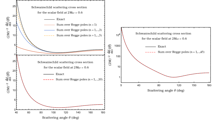
Figure 6: The scalar cross section of a Schwarzschild BH for $2M\omega=0.6$ and its Regge pole approximation.

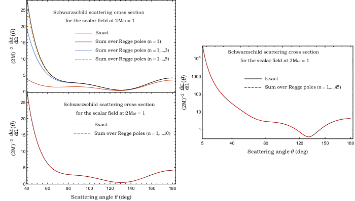
Figure 7: The scalar cross section of a Schwarzschild BH for $2M\omega=1$ and its Regge pole approximation.

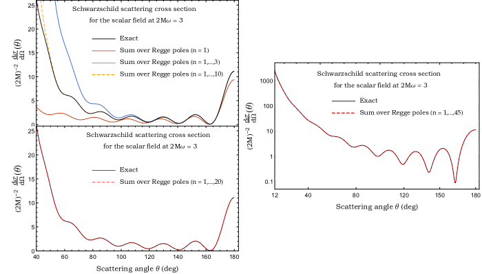
Figure 8: The scalar cross section of a Schwarzschild BH for $2M\omega=3$ and its Regge pole approximation.

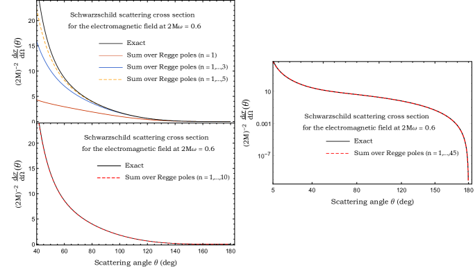
Figure 12: The electromagnetic cross section of a Schwarzschild BH for $2M\omega=0.6$ and its Regge pole approximation.

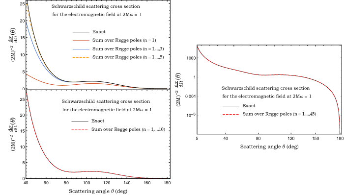
Figure 13: The electromagnetic cross section of a Schwarzschild BH for $2M\omega=1$ and its Regge pole approximation.

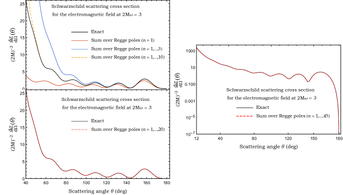
Figure 14: The electromagnetic cross section of a Schwarzschild BH for $2M\omega=3$ and its Regge pole approximation.

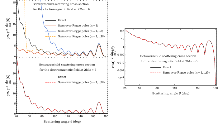
Figure 15: The electromagnetic cross section of a Schwarzschild BH for $2M\omega=6$ and its Regge pole approximation.

In Figs. 4-9, we focus on the scalar field and we compare the differential scattering cross section (1) constructed from the partial wave expansion (2) with its Regge pole approximation obtained from the Regge pole sum (II.2.3). In Figs. 10-15 we focus on the electromagnetic field and we compare the differential scattering cross section (3) constructed from the partial wave expansion (4)-(6) with its Regge pole approximation obtained from the Regge pole sum (II.3.2). The comparisons are achieved for the reduced frequencies $2M\omega=$ 0.1, 0.3, 0.6, 1, 3 and 6 and, for these frequencies, we have displayed the lowest Regge poles and the associated residues in Table 1 (for the scalar field ) and in Table 2 (for the electromagnetic field). The higher Regge poles and their residues that have been necessary to obtain some of the results displayed in Figs. 4-15 are available upon request from the authors.

In Figs. 6-9 and 12-15, we display the results obtained for intermediate and high reduced frequencies (here, we consider the reduced frequencies $2M\omega=$ 0.6, 1, 3 and 6). We can observe that, in the “short”-wavelength regime, the Regge pole approximation involving a small number of Regge poles permits us to describe very well the cross sections for intermediate and large values of the scattering angle and, in particular, the BH glory. Taking into account additional Regge poles improves the Regge pole approximation and we can see that, by summing over a large number of Regge poles, the whole scattering cross section is impressively described, this being valid even for small scattering angles.

It is important to note that, for “high” reduced frequencies, it is not necessary to take into account the background integrals in order to reproduce the differential scattering cross sections. In fact, we can numerically obtain these contributions and observe that they are completely negligible for intermediate and large scattering angles. It seems they begin to play a role only for small angles. In Table 3, we have considered, for the electromagnetic field at $2M\omega=1$, the various contributions to the CAM representation (38). We can see that, for the scattering angles $\theta=15\degree$ and $\theta=20\degree$, the background integrals, although not completely negligible, play a minor role. It would be interesting to check if this remains valid even for scattering angles $\theta\ll 1/(2M\omega)$ but, due to numerical instabilities when $\theta\to 0$, we are not currently able to provide such a result.

In Figs. 4, 5, 10 and 11, we focus on the results obtained for low reduced frequencies (here, we consider the reduced frequencies $2M\omega=$ 0.1 and 0.3). We can observe that, in the long-wavelength regime, the Regge pole approximations (II.2.3) and (II.3.2) alone do not permit us to reconstruct the differential scattering cross sections but that this can be achieved by taking into account the background integral contributions (27) and (39).

Table 1: The lowest Regge poles $\lambda_{n}(\omega)$ for the scalar field and the associated residues $r_{n}(\omega)$. We assume $2M=1$.

$n$	$\omega$	$\lambda_{n}(\omega)$	$r_{n}(\omega)$
$1$	$0.1$	$\phantom{1}0.299705+0.532035i$	$\phantom{-}0.110788-0.088226i$
	$0.3$	$\phantom{1}0.768159+0.531039i$	$\phantom{-}0.229999-0.159051i$
	$0.6$	$\phantom{1}1.543385+0.511888i$	$\phantom{-}0.389142-0.125974i$
	$1$	$\phantom{1}2.586845+0.504736i$	$\phantom{-}0.527572+0.019732i$
	$3$	$\phantom{1}7.790118+0.500553i$	$-0.136670+0.901886i$
	$6$	$15.586384+0.500139i$	$-0.594258-1.144512i$
$2$	$0.1$	$\phantom{1}0.495889+1.176250i$	$\phantom{-}0.099116-0.087234i$
	$0.3$	$\phantom{1}0.976977+1.364123i$	$\phantom{-}0.119559-0.228260i$
	$0.6$	$\phantom{1}1.695146+1.448184i$	$\phantom{-}0.181312-0.487058i$
	$1$	$\phantom{1}2.688355+1.479587i$	$\phantom{-}0.447998-0.888968i$
	$3$	$\phantom{1}7.825611+1.497769i$	$\phantom{-}4.596565+1.422003i$
	$6$	$15.604187+1.499447i$	$-12.419829+5.305460i$
$3$	$0.1$	$\phantom{1}0.650192+1.778513i$	$\phantom{-}0.087664-0.087739i$
	$0.3$	$\phantom{1}1.164769+2.098578i$	$\phantom{-}0.056734-0.236550i$
	$0.6$	$\phantom{1}1.878969+2.288202i$	$-0.078148-0.527337i$
	$1$	$\phantom{1}2.843093+2.391435i$	$-0.357084-1.170498i$
	$3$	$\phantom{1}7.893803+2.484084i$	$\phantom{-}7.751902-10.715411i$
	$6$	$15.639426+2.495896i$	$\phantom{-}16.758993+69.494273i$
$4$	$0.1$	$\phantom{1}0.788665+2.349868i$	$\phantom{-}0.079894-0.087791i$
	$0.3$	$\phantom{1}1.339372+2.783917i$	$\phantom{-}0.016812-0.232342i$
	$0.6$	$\phantom{1}2.065320+3.068702i$	$-0.245770-0.466956i$
	$1$	$\phantom{1}3.018870+3.248630i$	$-0.987253-0.88251i$
	$3$	$\phantom{1}7.990039+3.454396i$	$-11.471634-23.211359i$
	$6$	$15.691407+3.487740i$	$\phantom{-}256.923913+5.083667i$
$5$	$0.1$	$\phantom{1}0.917562+2.899702i$	$\phantom{-}0.074199-0.087641i$
	$0.3$	$\phantom{1}1.504128+3.437384i$	$-0.011069-0.224974i$
	$0.6$	$\phantom{1}2.248056+3.809074i$	$-0.348103-0.384562i$
	$1$	$\phantom{1}3.201835+4.063591i$	$-1.301089-0.421317i$
	$3$	$\phantom{1}8.109029+4.405790i$	$-40.72701-6.755946i$
	$6$	$15.759163+4.473447i$	$\phantom{-}251.611779-664.675235i$
$6$	$0.1$	$\phantom{1}1.039655+3.433425i$	$\phantom{-}0.069763-0.087418i$
	$0.3$	$\phantom{1}1.661166+4.067794i$	$-0.031853-0.216897i$
	$0.6$	$\phantom{1}2.425852+4.520191i$	$-0.410128-0.302558i$
	$1$	$\phantom{1}3.386161+4.845810i$	$-1.384667+0.028934i$
	$3$	$\phantom{1}8.245770+5.337166i$	$-45.341516+35.668449i$
	$6$	$15.841536+5.451746i$	$-1147.818563-1147.131306i$
$7$	$0.1$	$\phantom{1}1.156528+3.954439i$	$\phantom{-}0.066156-0.087170i$
	$0.3$	$\phantom{1}1.811951+4.680400i$	$-0.048060-0.208882i$
	$0.6$	$\phantom{1}2.598670+5.208747i$	$-0.446908-0.227138i$
	$1$	$\phantom{1}3.569316+5.602015i$	$-1.328185+0.409299i$
	$3$	$\phantom{1}8.396000+6.248658i$	$-12.517767+72.751731i$
	$6$	$15.937250+6.421641i$	$-3071.847422+904.87469i$
$8$	$0.1$	$\phantom{1}1.269207+4.465047i$	$\phantom{-}0.063133-0.086918i$
	$0.3$	$\phantom{1}1.957532+5.278644i$	$-0.061116-0.201188i$
	$0.6$	$\phantom{1}2.766835+5.879184i$	$-0.467343-0.159566i$
	$1$	$\phantom{1}3.750196+6.337011i$	$-1.193204+0.709887i$
	$3$	$\phantom{1}8.556293+7.141111i$	$\phantom{-}41.280909+78.754435i$
	$6$	$16.044990+7.382406i$	$-1576.690323+5414.570984i$
$9$	$0.1$	$\phantom{1}1.378403+4.966897i$	$\phantom{-}0.060539-0.086669i$
	$0.3$	$\phantom{1}2.098692+5.864936i$	$-0.071892-0.193894i$
	$0.6$	$\phantom{1}2.930753+6.534615i$	$-0.476862-0.099550i$
	$1$	$\phantom{1}3.928352+7.054311i$	$-1.017928+0.937403i$
	$3$	$\phantom{1}8.723992+8.015714i$	$\phantom{-}89.972545+49.380751i$
	$6$	$16.163453+8.333555i$	$\phantom{-}5509.049968+7209.509940i$

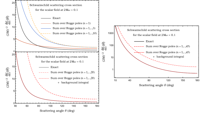
Figure 4: The scalar cross section of a Schwarzschild BH for $2M\omega=0.1$, its Regge pole approximation and the background integral contribution.

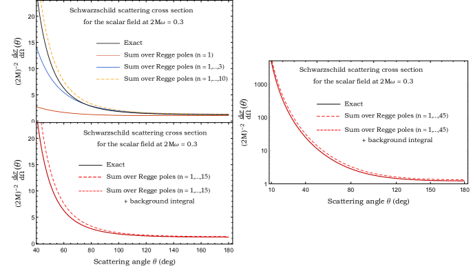
Figure 5: The scalar cross section of a Schwarzschild BH for $2M\omega=0.3$, its Regge pole approximation and the background integral contribution.

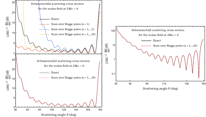
Figure 9: The scalar cross section of a Schwarzschild BH for $2M\omega=6$ and its Regge pole approximation.

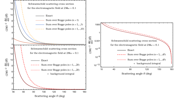
Figure 10: The electromagnetic cross section of a Schwarzschild BH for $2M\omega=0.1$, its Regge pole approximation and the background integral contribution.

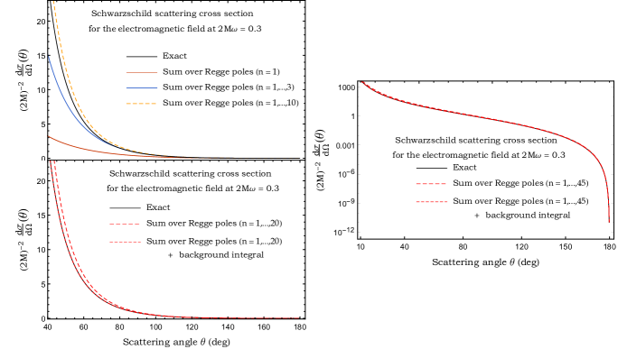
Figure 11: The electromagnetic cross section of a Schwarzschild BH for $2M\omega=0.3$, its Regge pole approximation and the background integral contribution.

Table 2: The lowest Regge poles $\lambda_{n}(\omega)$ for the electromagnetic field and the associated residues $r_{n}(\omega)$. We assume $2M=1$.

$n$	$\omega$	$\lambda_{n}(\omega)$	$r_{n}(\omega)$
$1$	$0.1$	$\phantom{1}0.610235+0.1857157i$	$0.141533+0.042574i$
	$0.3$	$\phantom{1}1.022046+0.3598438i$	$0.261310-0.042212i$
	$0.6$	$\phantom{1}1.719903+0.4428220i$	$0.383610-0.048683i$
	$1$	$\phantom{1}2.705358+0.475454i$	$0.508191+0.067329i$
	$3$	$\phantom{1}7.832474+0.496948i$	$-0.159996+0.894283i$
	$6$	$15.607716+0.499228i$	$-0.578675-1.150971i$
$2$	$0.1$	$\phantom{1}0.525188+1.002194i$	$0.125937-0.097912i$
	$0.3$	$\phantom{1}1.041088+1.218701i$	$0.159661-0.245504i$
	$0.6$	$\phantom{1}1.778902+1.346966i$	$0.242164-0.499689i$
	$1$	$\phantom{1}2.769262+1.419171i$	$0.526456-0.877988i$
	$3$	$\phantom{1}7.865654+1.487542i$	$4.568657+1.545802i$
	$6$	$15.62521+1.496753i$	$-12.494555+5.146258i$
$3$	$0.1$	$\phantom{1}0.662252+1.674293i$	$0.095812-0.093134i$
	$0.3$	$\phantom{1}1.190599+2.002822i$	$0.065892-0.251733i$
	$0.6$	$\phantom{1}1.919344+2.206835i$	$-0.064979-0.560444i$
	$1$	$\phantom{1}2.892291+2.330093i$	$-0.325379-1.231546i$
	$3$	$\phantom{1}7.929898+2.468721i$	$8.065346-10.612212i$
	$6$	$15.65986+2.491532i$	$15.910509+69.844271i$
$4$	$0.1$	$\phantom{1}0.795653+2.274956i$	$\phantom{-}0.083712-0.091011i$
	$0.3$	$\phantom{1}1.353709+2.713393i$	$\phantom{-}0.018874-0.241698i$
	$0.6$	$\phantom{1}2.088487+3.004734i$	$-0.250327-0.488373i$
	$1$	$\phantom{1}3.049989+3.194709i$	$-1.005893-0.931457i$
	$3$	$\phantom{1}8.021481+3.435669i$	$-11.138536-23.703501i$
	$6$	$15.711016+3.481878i$	$257.725106+8.206397i$
$5$	$0.1$	$\phantom{1}0.922279+2.841097i$	$\phantom{-}0.076365-0.089785i$
	$0.3$	$\phantom{1}1.513455+3.381624i$	$-0.011075-0.231005i$
	$0.6$	$\phantom{1}2.263145+3.757064i$	$-0.356562-0.396595i$
	$1$	$\phantom{1}3.22292+4.017259i$	$-1.333866-0.443471i$
	$3$	$\phantom{1}8.135861+4.385262i$	$-41.163827-7.491406i$
	$6$	$15.77777+4.466296i$	$260.251292-664.857185i$
$6$	$0.1$	$\phantom{1}1.043127+3.385241i$	$\phantom{-}0.071135-0.088951i$
	$0.3$	$\phantom{1}1.667826+4.021677i$	$-0.032532-0.221005i$
	$0.6$	$\phantom{1}2.436547+4.476543i$	$-0.418506-0.308999i$
	$1$	$\phantom{1}3.401342+4.805736i$	$-1.41496+0.025197i$
	$3$	$\phantom{1}8.268455+5.315989i$	$-46.408075+35.620183i$
	$6$	$15.859025+5.443533i$	$-1142.290033-1165.297141i$
$7$	$0.1$	$\phantom{1}1.159231+3.913502i$	$\phantom{-}0.067092-0.088324i$
	$0.3$	$\phantom{1}1.817004+4.641067i$	$-0.048946-0.211809i$
	$0.6$	$\phantom{1}2.606707+5.171198i$	$-0.454210-0.230350i$
	$1$	$\phantom{1}3.580784+5.566912i$	$-1.351547+0.415443i$
	$3$	$\phantom{1}8.41515+6.227581i$	$-13.342348+73.643709i$
	$6$	$15.953564+6.412592i$	$-3099.407958+881.950573i$
$8$	$0.1$	$\phantom{1}1.271395+4.429445i$	$\phantom{-}0.063805-0.087819i$
	$0.3$	$\phantom{1}1.961534+5.244345i$	$-0.062033-0.203348i$
	$0.6$	$\phantom{1}2.773137+5.846253i$	$-0.473449-0.160898i$
	$1$	$\phantom{1}3.759191+6.305865i$	$-1.209644+0.720509i$
	$3$	$\phantom{1}8.572514+7.120576i$	$41.311379+80.054461i$
	$6$	$16.060119+7.372728i$	$-1632.012756+5438.076537i$
$9$	$0.1$	$\phantom{1}1.380226+4.935390i$	$\phantom{-}0.061041-0.087394i$
	$0.3$	$\phantom{1}2.101964+5.834520i$	$-0.072774-0.195533i$
	$0.6$	$\phantom{1}2.935855+6.505296i$	$-0.481896-0.099774i$
	$1$	$\phantom{1}3.935619+7.026361i$	$-1.028681+0.949498i$
	$3$	$\phantom{1}8.737816+7.995955i$	$90.843271+50.395101i$
	$6$	$16.177423+8.323434i$	$5495.804514+7300.293176i$

Table 3: We compare, for the electromagnetic field at $\omega=1$ ($2M=1$), the exact value of the scattering amplitude (4) with the sum over Regge poles (II.3.2) and we highlight the minor role of the background integral contributions (39) and (39a).

Electromagnetic field at $\omega=1$ ($2M=1$)	$\theta=15\degree$	$\theta=20\degree$
$|A(\omega,\theta)|^{2}$	$1023.0681$	$335.2717$
$|A^{\text{\tiny{RP}}}(\omega,\theta)|^{2}$ (n=1,…, 60)	$1025.5432$	$335.8305$
$|A^{\text{\tiny{RP}}}(\omega,\theta)|^{2}$ (n=1,…, 90)	$1025.4676$	$335.8343$
$|A^{\text{\tiny{B},\tiny{Re}}}(\omega,\theta)+A^{\text{\tiny{RP}}}(\omega,\theta)|^{2}$ (n=1,…, 90)	$1023.0754$	$335.2743$
$|A^{\text{\tiny{B}}}(\omega,\theta)+A^{\text{\tiny{RP}}}(\omega,\theta)|^{2}$ (n=1,…, 90)	$1023.0762$	$335.2718$

IV BH glory and orbiting oscillations

In this section, we provide an analytical description of both the glory and orbiting cross sections based on the Regge pole sums (II.2.3) and (II.3.2). This is achieved by inserting in these sums analytical approximations for the lowest Regge poles and the associated residues. These approximations are obtained by assuming that, at large reduced frequencies $2M\omega$, the lowest Regge poles are in a one-to-one correspondence with “surface waves” propagating close to the unstable circular photon (graviton) orbit at $r=3M$, i.e., near the Schwarzschild photon sphere Decanini et al. (2003); Decanini and Folacci (2010); Dolan and Ottewill (2009); Decanini et al. .

IV.1 Remarks concerning backward glory scattering and orbiting scattering

It is well known that, for intermediate and high reduced frequencies, two interesting structures which are associated “classically/semiclassically” with backward glory scattering and orbiting scattering can be observed in the plots of BH cross sections (see, e.g., Ref. Futterman et al. (2012) or Chap. 4 of Ref. Frolov and Novikov (1998) and references therein). Roughly speaking, we can consider that glory scattering explains the behavior of the cross section in the backward direction, i.e., for scattering angles $\theta\approx\pi$ and that orbiting scattering permits us to understand the oscillations arising for “intermediate” scattering angles. A pioneering analysis, in the context of BH physics, of these two phenomena, can be found in an article by Handler and Matzner Handler and Matzner (1980). It is based on ideas developed by Ford and Wheeler in their semiclassically study of quantum mechanical scattering Ford and Wheeler (1959). A deeper analysis based on path integration has been carried out by DeWitt-Morette and co-workers Matzner et al. (1985); Anninos et al. (1992) leading to semiclassical analytic formulas.

In Ref. Matzner et al. (1985), the authors have established that, for a Schwarzschild BH, the glory scattering cross section of massless waves of spin $s$ can be approximated by

$$\left.\frac{d\sigma}{d\Omega}\right|_{\mathrm{glory}}=30.752M^{3}\omega\,\left[J_{2s}\left(5.357M\omega\sin\theta\right)\right]^{2},$$ (41)

a formula which is formally valid for $2M\omega\gg 1$ and $|\theta-\pi|\ll 1$. Here, $J_{2s}$ is a Bessel function of the first kind. It should be noted that (41) encodes only the contribution of the first backward glory and that the numerical factors appearing in this approximation are those obtained in Ref. Crispino et al. (2009b). It is moreover interesting to recall that, in Ref. Anninos et al. (1992), the authors have proposed a formula which roughly describes the orbiting oscillations of the scalar cross section. In our opinion, we cannot be satisfied with that formula. Indeed, it involves two free parameters which must be adjusted and, even if this job is done effectively, it does not permit us to reproduce with good agreement the exact result (see Fig. 9 of Ref. Anninos et al. (1992)).

IV.2 Analytical Regge pole approximations of scattering amplitudes

As we shall see, it is possible from Regge pole sums to describe analytically both phenomena, i.e., to establish a unique formula which fits the glory and orbiting cross sections. At first sight, this is rather surprising because, in the geometrical-optics limit (i.e., if we only focus on the concepts of geodesic and bundle of geometrical rays), the two phenomena are very different in that they are associated with very different mathematical behavior of the deflection function Ford and Wheeler (1959); Handler and Matzner (1980); Matzner et al. (1985); Anninos et al. (1992). But, here, we must not be too obsessed by classical results. Indeed, we are working in the framework of wave physics and it is tempting to consider that the glory and orbiting effects are not fundamentally different insofar as they are both generated by the excitation of surface waves propagating close to the BH photon sphere. By using the Regge pole approach of BH physics, we can take into account these diffractive effects due to the Schwarzschild photon sphere Andersson (1994); Decanini et al. (2003); Decanini and Folacci (2010); Dolan and Ottewill (2009); Decanini et al. (2010) and derive asymptotic expansions for the Regge poles and the associated residues.

Analytical expressions for the lowest Regge poles of the Schwarzschild BH have been obtained in Ref. Decanini and Folacci (2010). This has been achieved by using a third-order WKB approximation to solve the Regge-Wheeler equation (7)-(8) or, more precisely, by extending to Regge poles the approach developed in the context of the determination of the QNMs by Schutz and Will Schutz and Will (1985) and by Iyer and Will Iyer and Will (1987); Iyer (1987). It should be noted that it is possible to go beyond the third-order WKB approximation (see Refs. Dolan and Ottewill (2009); Decanini et al. (2011a)) but here we will not need these improved results. In fact, we shall only consider that, at large $2M\omega$, the lowest Regge poles closely adhere to the asymptotic form

$$\lambda_{n}(\omega)\approx 3\sqrt{3}\,M\omega+i\,(n-1/2)+\frac{\sqrt{3}\,a_{n}}{18M\omega}$$ (42)

[here we have neglected the terms of order $1/(2M\omega)^{2}$ derived in Ref. Decanini and Folacci (2010)] where

$$a_{n}=\frac{2}{3}\left[\frac{5}{12}(n-1/2)^{2}+\frac{115}{144}-1+s^{2}\right].$$ (43)

It is moreover possible to obtain an analytical expression for the residues associated with the lowest Regge poles of the Schwarzschild BH. By extending to Regge poles the calculations which have permitted to Dolan and Ottewill to derive an analytical expression for the QNM excitation factors Dolan and Ottewill (2011), we have obtained Decanini et al.

$$r_{n}(\omega)\approx\frac{\left[-i\,216(3\sqrt{3}M\omega)/\xi\right]^{n-1/2}}{\sqrt{2\pi}\,(n-1)!}e^{i2M\omega y}e^{i\pi\lambda_{n}(\omega)}$$

where

$$\xi=7+4\sqrt{3}\quad\mathrm{and}\quad y=3-3\sqrt{3}+4\ln 2-3\ln\xi.$$ (45)

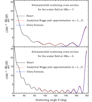
Figure 16: The scalar cross section of a Schwarzschild BH for $2M\omega=3$ and $2M\omega=6$. We compare the exact result with the glory formula and with that obtained from the analytical Regge pole approximation.

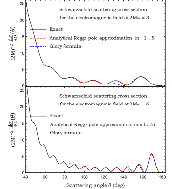
Figure 17: The electromagnetic cross section of a Schwarzschild BH for $2M\omega=3$ and $2M\omega=6$. We compare the exact result with the glory formula and with that obtained from the analytical Regge pole approximation.

By inserting now the approximations (42)-(43) for the Regge poles and (IV.2)-(45) for the residues into the Regge pole sum (II.2.3) for the scalar field and into the Regge pole sum (II.3.2) for the electromagnetic field, we have at our disposal analytical approximations for the scattering cross sections associated with these two fields which are formally valid for $2M\omega\to+\infty$. It should be however noted that the Regge pole sums considered can only involve a small number of terms because the approximations (42) and (IV.2) are accurate only for the lowest Regge poles. As a consequence, from a theoretical point of view, our analytical Regge pole approximations cannot describe the cross sections for small scattering angles.

IV.3 Results and comments

In Figs. 16 and 17, we complete our study of Sec. III.2 by now comparing the exact scattering cross sections with their analytical approximations constructed in Sec. IV.2. The comparisons are achieved for the reduced frequencies $2M\omega=3$ and 6 and the summations are over the first five Regge poles. We can observe that the analytical Regge pole approximations permit us to reproduce with very good agreement both the glory cross section and a large part of the orbiting cross section. It is moreover surprising to note that, by considering analytical Regge pole sums involving a large number of terms, we are able to describe the cross sections in a wide range of scattering angles despite the inaccuracy of the approximations (42) and (IV.2) for the higher Regge poles (see Fig. 18 where we have considered the case of the scalar field at $2M\omega=6$).

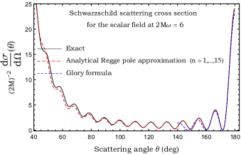
Figure 18: The scalar cross section of a Schwarzschild BH for $2M\omega=6$. We compare the exact result with the glory formula and with that obtained from the analytical Regge pole approximation where we sum over a large number of terms despite the inaccuracy of the approximations (42) and (IV.2) for the higher Regge poles.

V Conclusion

In this article, we have considered the scattering of scalar and electromagnetic waves by a Schwarzschild BH by focusing on the associated differential scattering cross sections and we have shown that, for intermediate and high reduced frequencies, these cross sections can be reconstructed in terms of Regge poles with great precision. This is really surprising and certainly due to the fact that BHs are very particular physical objects. Indeed, in quantum mechanics de Alfaro and Regge (1965); Newton (1982), electromagnetism and optics Watson (1918); Sommerfeld (1949); Newton (1982); Nussenzveig (1992); Grandy (2000) and acoustics Überall (1992), background integral contributions are never negligible (this remains true regardless of the frequency) and, as a consequence, a Regge pole sum alone does not permit us to reproduce a differential scattering cross section. In the context of scattering of scalar and electromagnetic waves by a Schwarzschild BH, we have observed that it is necessary to take into account background integral contributions only for low reduced frequencies.

In the short-wavelength regime, from Regge pole sums we have also been able to describe numerically, with an impressive agreement, the BH glory occurring in the backward direction as well as the orbiting oscillations appearing on the differential scattering cross sections for small and intermediate scattering angles. Moreover, it is important to note that working with Regge pole sums has permitted us to overcome the difficulties linked to the lack of convergence of the partial wave expansions defining the cross sections which are due to the long-range nature of the fields propagating on a Schwarzschild background.

Finally, taking into account the fact that, in the short-wavelength regime, a Regge pole sum encodes the physical information hidden into the partial wave expansion defining a differential scattering cross section, we have derived an analytical approximation fitting both the BH glory and a large part of the orbiting oscillations. This has been achieved by inserting into the Regge pole sum asymptotic approximations for the lowest Regge poles and the associated residues. In our opinion, our analytical approximation is far superior to existing formulas Matzner et al. (1985); Anninos et al. (1992).

We hope in next works to extend our study to scattering of gravitational waves by a Schwarzschild BH as well as to scattering of waves by a Kerr BH (see Refs. Matzner and Ryan (1977, 1978); Handler and Matzner (1980); Glampedakis and Andersson (2001); Dolan (2008b, a) for articles concerning these two topics and which could serve as departure points for such works).

*

Appendix A Iterative method to accelerate the convergence of background integrals

Due to the long-range nature of the fields propagating on a Schwarzschild BH, the background integrals (27b) and (39) suffer a lack of convergence. In this Appendix we explain how to overcome this problem, i.e., how to accelerate their convergence. In fact, the same problem occurs for the partial wave expansions (2), (5) and (4) (see, e.g., Refs. Anninos et al. (1992) where the case of the scalar field is discussed). For these partial wave expansions, the convergence can be obtained by employing an iterative method introduced a long time ago in the context of Coulomb scattering by Yennie, Ravenhall and Wilson Yennie et al. (1954) [see also Refs. Dolan (2008a); Crispino et al. (2009a) where this method is used in the context of scattering by BHs and see, e.g., Ref. Anninos et al. (1992) for another approach based on the truncation of partial wave expansions and on the matching of the Schwarzschild $S$-matrix elements $S_{\ell}(\omega)$ with the Newtonian ones]. In this Appendix, we briefly recall this iterative method because we use it in Sec. III in order to accelerate the convergence of the partial wave expansions (2) and (5) and we generalize it in order to deal with the background integrals (27b) and (39).

A.1 Acceleration of the convergence of partial wave expansions

In order to improve the convergence of the partial wave expansion

$$\alpha(\theta)=\sum_{\ell=0}^{\infty}a_{\ell}\,P_{\ell}(\cos\theta)$$ (46)

[see Eqs. (2) and (5)] we introduce the associated “reduced” series Yennie et al. (1954)

$${\widetilde{\alpha}}^{(n)}(\theta)=\sum_{\ell=0}^{\infty}{\widetilde{a}}^{(n)}_{\ell}\,P_{\ell}(\cos\theta)$$ (47)

defined by

$$\alpha(\theta)=(1-\cos\theta)^{-n}\,{\widetilde{\alpha}}(\theta).$$ (48)

It should be noted that, by reexpressing the series (46) in the form (48), we isolate the pathological behavior of the partial wave expansions (2) and (5) occurring for $\theta\to 0$. By using now the recursion relation Abramowitz and Stegun (1965)

$$(\ell+1)P_{\ell+1}(\cos\theta)-(2\ell+1)\cos\theta P_{\ell}(\cos\theta)$$

$$\qquad\qquad+\ell P_{\ell-1}(\cos\theta)=0$$ (49)

in the form

$$(1-\cos\theta)P_{\ell}(\cos\theta)=P_{\ell}(\cos\theta)$$

$$\quad-\frac{\ell+1}{2\ell+1}P_{\ell+1}(\cos\theta)-\frac{\ell}{2\ell+1}P_{\ell-1}(\cos\theta)$$ (50)

we can show from (46)–(48) that the coefficients ${\widetilde{a}}^{(n)}_{\ell}$ can be expressed in terms of the coefficients ${\widetilde{a}}^{(n-1)}_{\ell}$. We have, for $\ell\in\mathbb{N}$,

$${\widetilde{a}}^{(n)}_{\ell}={\widetilde{a}}^{(n-1)}_{\ell}-\frac{\ell+1}{2\ell+3}{\widetilde{a}}^{(n-1)}_{\ell+1}-\frac{\ell}{2\ell-1}{\widetilde{a}}^{(n-1)}_{\ell-1}$$ (51)

(here we take ${\widetilde{a}}^{(n-1)}_{-1}=0$). As noted in Ref. Yennie et al. (1954), we have for large values of $\ell$,

$${\widetilde{a}}^{(n)}_{\ell}={\cal O}\left({\widetilde{a}}^{(n-1)}_{\ell}/\ell^{2}\right).$$ (52)

This explicitly shows that using the reduced series (47) greatly improves the convergence of the initial partial wave expansion (46).

A.2 Acceleration of the convergence of background integrals

In order to improve the convergence of the background integral

$$\alpha(\theta)=\int_{0}^{+\infty}d\lambda\,a(\lambda)\,Q_{\lambda-1/2}(\cos\theta+i0)$$ (53)

[see Eqs. (27b) and (39)], we first split it in the form

$$\alpha(\theta)=\int_{0}^{\lambda_{0}}d\lambda\,a(\lambda)\,Q_{\lambda-1/2}(\cos\theta+i0)+\alpha_{\lambda_{0}}(\theta)$$ (54)

where

$$\alpha_{\lambda_{0}}(\theta)=\int_{\lambda_{0}}^{+\infty}d\lambda\,a(\lambda)\,Q_{\lambda-1/2}(\cos\theta+i0).$$ (55)

The choice of the truncation parameter ${\lambda_{0}}$ will be discussed later. We then introduce the “reduced” integrals ${\widetilde{\alpha}}_{\lambda_{0}}^{(n)}(\theta)$ defined by

$$\alpha_{\lambda_{0}}(\theta)=(1-\cos\theta)^{-n}\,{\widetilde{\alpha}}_{\lambda_{0}}^{(n)}(\theta).$$ (56)

By using the relation

$$(1-\cos\theta)Q_{\lambda-1/2}(\cos\theta+i0)=Q_{\lambda-1/2}(\cos\theta+i0)$$

$$\qquad-\left(\frac{\lambda+1/2}{2\lambda}\right)Q_{\lambda+1/2}(\cos\theta+i0)$$

$$\qquad-\left(\frac{\lambda-1/2}{2\lambda}\right)Q_{\lambda-3/2}(\cos\theta+i0)$$ (57)

which is a consequence of the definition (II.2.3) and of the relation Abramowitz and Stegun (1965)

$$(\nu+1)P_{\nu+1}(\cos\theta)-(2\nu+1)\cos\theta P_{\nu}(\cos\theta)$$ (58)

$$\qquad\qquad+\nu P_{\nu-1}(\cos\theta)=0,$$

we can show that these reduced integrals can be written in the form

$${\widetilde{\alpha}}_{\lambda_{0}}^{(n)}(\theta)=\int_{\lambda_{0}}^{+\infty}d\lambda\,{\widetilde{a}}^{(n)}(\lambda)\,Q_{\lambda-1/2}(\cos\theta+i0)+{\widetilde{R}}^{(n)}(\theta)$$ (59)

where ${\widetilde{R}}^{(n)}(\theta)$ is an integral over a finite integration domain which can be expressed in terms of the integral ${\widetilde{R}}^{(n-1)}(\theta)$ and where the function ${\widetilde{a}}^{(n)}(\lambda)$ can be expressed in terms of the function ${\widetilde{a}}^{(n-1)}(\lambda)$. We have

$${\widetilde{a}}^{(n)}(\lambda)={\widetilde{a}}^{(n-1)}(\lambda)-\left(\frac{\lambda+1/2}{2(\lambda+1)}\right){\widetilde{a}}^{(n-1)}(\lambda+1)$$

$$\qquad\qquad-\left(\frac{\lambda-1/2}{2(\lambda-1)}\right){\widetilde{a}}^{(n-1)}(\lambda-1)$$ (60)

and

$${\widetilde{R}}^{(n)}(\theta)=(1-\cos\theta){\widetilde{R}}^{(n-1)}(\theta)$$

$$\quad+\int_{\lambda_{0}-1}^{\lambda_{0}}d\lambda\left[\left(\frac{\lambda+1/2}{2\lambda}\right){\widetilde{a}}^{(n-1)}(\lambda)\,Q_{\lambda+1/2}(\cos\theta+i0)\right.$$

$$\qquad\left.-\left(\frac{\lambda+1/2}{2(\lambda+1)}\right){\widetilde{a}}^{(n-1)}(\lambda+1)\,Q_{\lambda-1/2}(\cos\theta+i0)\right].$$

From the relation (A.2) we can see that, for large values of $\lambda$,

$${\widetilde{a}}^{(n)}(\lambda)={\cal O}\left({\widetilde{a}}^{(n-1)}(\lambda)/\lambda^{2}\right).$$ (62)

This explicitly shows that using the reduced integral (59) greatly improves the convergence of the initial background integral (53). As far as the choice of the truncation parameter ${\lambda_{0}}$ is concerned, it should be noted that it depends on the number $n$ of iterations performed. Indeed, due to the shift of the variable $\lambda$ induced by the relation (A.2), we can observe that ${\widetilde{a}}^{(n)}(\lambda)$ is not defined for $\lambda\in[0,n[$ and, in order to have the integrals (A.2) and (59) well defined, it is necessary to take $\lambda_{0}\geq n$.

References

- Futterman et al. (2012) J. A. H. Futterman, F. A. Handler, and R. A. Matzner, Scattering from Black Holes, Cambridge Monographs on Mathematical Physics (Cambridge University Press, 2012).
- Frolov and Novikov (1998) V. P. Frolov and I. D. Novikov, Black Hole Physics: Basic Concepts and New Developments, Fundamental Theories of Physics, Vol. 96 (Kluwer Academic Publishers, 1998).
- de Alfaro and Regge (1965) V. de Alfaro and T. Regge, Potential Scattering (North-Holland Publishing Company, Amsterdam, 1965).
- Newton (1982) R. G. Newton, Scattering Theory of Waves and Particles, 2nd ed. (Springer-Verlag, New York, 1982).
- Watson (1918) G. N. Watson, “The diffraction of electric waves by the Earth,” Proc. R. Soc. A 95, 83 (1918).
- Sommerfeld (1949) A. Sommerfeld, Partial Differential Equations of Physics (Academic Press, New York, 1949).
- Nussenzveig (1992) H. M. Nussenzveig, Diffraction Effects in Semiclassical Scattering (Cambridge University Press, Cambridge, 1992).
- Grandy (2000) W. T. Grandy, Scattering of Waves from Large Spheres (Cambridge University Press, Cambridge, 2000).
- Überall (1992) H. Überall, Acoustic Resonance Scattering (Gordon and Breach, New York, 1992).
- Aki and Richards (2002) K. Aki and P. Richards, Quantitative Seismology, 2nd ed. (University Science Book, Sausalito, 2002).
- Gribov (2003) V. N. Gribov, The Theory of Complex Angular Momenta: Gribov Lectures on Theoretical Physics (Cambridge University Press, Cambridge, 2003).
- Collins (1977) P. D. B. Collins, An Introduction to Regge Theory and High-Energy Physics (Cambridge University Press, Cambridge, 1977).
- Barone and Predazzi (2002) V. Barone and E. Predazzi, High-Energy Particle Diffraction (Springer-Verlag, Berlin, 2002).
- Donnachie et al. (2005) S. Donnachie, G. Dosch, P. V. Landshoff, and O. Nachtmann, Pomeron Physics and QCD (Cambridge University Press, Cambridge, 2005).
- Andersson and Thylwe (1994) N. Andersson and K. E. Thylwe, “Complex angular momentum approach to black hole scattering,” Class. Quant. Grav. 11, 2991 (1994).
- Andersson (1994) N. Andersson, “Complex angular momenta and the black hole glory,” Class. Quant. Grav. 11, 3003 (1994).
- Decanini et al. (2003) Y. Decanini, A. Folacci, and B. Jensen, “Complex angular momentum in black hole physics and the quasinormal modes,” Phys. Rev. D 67, 124017 (2003), arXiv:gr-qc/0212093 .
- Glampedakis and Andersson (2003) K. Glampedakis and N. Andersson, “Quick and dirty methods for studying black hole resonances,” Class. Quant. Grav. 20, 3441 (2003), arXiv:gr-qc/0304030 .
- Decanini and Folacci (2010) Y. Decanini and A. Folacci, “Regge poles of the Schwarzschild black hole: A WKB approach,” Phys. Rev. D 81, 024031 (2010), arXiv:0906.2601 [gr-qc] .
- Decanini and Folacci (2009) Y. Decanini and A. Folacci, “Quasinormal modes of the BTZ black hole are generated by surface waves supported by its boundary at infinity,” Phys. Rev. D 79, 044021 (2009), arXiv:0901.1642 [hep-th] .
- Dolan and Ottewill (2009) S. R. Dolan and A. C. Ottewill, “On an expansion method for black hole quasinormal modes and Regge poles,” Class. Quant. Grav. 26, 225003 (2009), arXiv:0908.0329 [gr-qc] .
- Decanini et al. (2010) Y. Decanini, A. Folacci, and B. Raffaelli, “Unstable circular null geodesics of static spherically symmetric black holes, Regge poles and quasinormal frequencies,” Phys. Rev. D 81, 104039 (2010), arXiv:1002.0121 [gr-qc] .
- Decanini et al. (2011a) Y. Decanini, A. Folacci, and B. Raffaelli, “Resonance and absorption spectra of the Schwarzschild black hole for massive scalar perturbations: A complex angular momentum analysis,” Phys. Rev. D 84, 084035 (2011a), arXiv:1108.5076 [gr-qc] .
- Decanini et al. (2011b) Y. Decanini, G. Esposito-Farese, and A. Folacci, “Universality of high-energy absorption cross sections for black holes,” Phys. Rev. D 83, 044032 (2011b), arXiv:1101.0781 [gr-qc] .
- Decanini et al. (2011c) Y. Decanini, A. Folacci, and B. Raffaelli, “Fine structure of high-energy absorption cross sections for black holes,” Class. Quant. Grav. 28, 175021 (2011c), arXiv:1104.3285 [gr-qc] .
- Dolan et al. (2012) S. R. Dolan, L. A. Oliveira, and L. C. B. Crispino, “Resonances of a rotating black hole analogue,” Phys. Rev. D 85, 044031 (2012), arXiv:1105.1795 [gr-qc] .
- Macedo et al. (2013) C. F. B. Macedo, L. C. S. Leite, E. S. Oliveira, S. R. Dolan, and L. C. B. Crispino, “Absorption of planar massless scalar waves by Kerr black holes,” Phys. Rev. D 88, 064033 (2013), arXiv:1308.0018 [gr-qc] .
- Nambu and Noda (2016) Y. Nambu and S. Noda, “Wave optics in black hole spacetimes: The Schwarzschild case,” Class. Quant. Grav. 33, 075011 (2016), arXiv:1502.05468 [gr-qc] .
- Folacci and Ould El Hadj (2018) A. Folacci and M. Ould El Hadj, “Alternative description of gravitational radiation from black holes based on the Regge poles of the -matrix and the associated residues,” Phys. Rev. D 98, 064052 (2018), arXiv:1807.09056 [gr-qc] .
- Benone et al. (2018) C. L. Benone, L. C. S. Leite, L. C. B. Crispino, and S. R. Dolan, “On-axis scalar absorption cross section of Kerr-Newman black holes: Geodesic analysis, sinc and low-frequency approximations,” Int. J. Mod. Phys. D 27, 1843012 (2018), arXiv:1809.08275 [gr-qc] .
- Matzner (1968) R. A. Matzner, “Scattering of massless scalar waves by a Schwarzschild “singularity”,” J. Math. Phys. 9, 163 (1968).
- Mashhoon (1973) B. Mashhoon, “Scattering of electromagnetic radiation from a black hole,” Phys. Rev. D 7, 2807 (1973).
- Mashhoon (1974) B. Mashhoon, “Electromagnetic scattering from a black hole and the glory effect,” Phys. Rev. D 10, 1059 (1974).
- Fabbri (1975) R. Fabbri, “Scattering and absorption of electromagnetic waves by a Schwarzschild black hole,” Phys. Rev. D 12, 933 (1975).
- Sanchez (1976) N. G. Sanchez, “Scattering of scalar waves from a Schwarzschild black hole,” J. Math. Phys. 17, 688 (1976).
- Sanchez (1978) N. G. Sanchez, “Elastic scattering of waves by a black hole,” Phys. Rev. D 18, 1798 (1978).
- Matzner et al. (1985) R. A. Matzner, C. DeWitt-Morette, B. Nelson, and T.-R. Zhang, “Glory scattering by black holes,” Phys. Rev. D 31, 1869 (1985).
- Anninos et al. (1992) P. Anninos, C. DeWitt-Morette, R. A. Matzner, P. Yioutas, and T. R. Zhang, “Orbiting cross-sections: Application to black hole scattering,” Phys. Rev. D 46, 4477 (1992).
- Andersson (1995) N. Andersson, “Scattering of massless scalar waves by a Schwarzschild black hole: A phase integral study,” Phys. Rev. D 52, 1808 (1995).
- Glampedakis and Andersson (2001) K. Glampedakis and N. Andersson, “Scattering of scalar waves by rotating black holes,” Class. Quant. Grav. 18, 1939 (2001), arXiv:gr-qc/0102100 .
- Dolan (2008a) S. R. Dolan, “Scattering and absorption of gravitational plane waves by rotating black holes,” Class. Quant. Grav. 25, 235002 (2008a), arXiv:0801.3805 [gr-qc] .
- Crispino et al. (2009a) L. C. B. Crispino, S. R. Dolan, and E. S. Oliveira, “Electromagnetic wave scattering by Schwarzschild black holes,” Phys. Rev. Lett. 102, 231103 (2009a), arXiv:0905.3339 [gr-qc] .
- Falcke et al. (2000) H. Falcke, F. Melia, and E. Agol, “Viewing the shadow of the black hole at the galactic center,” Astrophys. J. 528, L13 (2000), arXiv:astro-ph/9912263 .
- Castelvecchi (2017) D. Castelvecchi, “How to hunt for a black hole with a telescope the size of Earth,” Nature 543, 478 (2017).
- Collaboration (2019) The Event Horizon Telescope Collaboration, “First M87 Event Horizon Telescope Results. I. The Shadow of the Supermassive Black Hole,” Astrophys. J. Lett. 875, L1 (2019).
- Goebel (1972) C. J. Goebel, “Comments on the “vibrations” of a black hole,” Astrophys. J. 172, L95 (1972).
- (47) Y. Decanini, A. Folacci, and M. Ould El Hadj, “Regge mode excitation and strong gravitational lensing (work in progress),” .
- Yennie et al. (1954) D. R. Yennie, D. G. Ravenhall, and R. N. Wilson, “Phase-shift calculation of high-energy electron scattering,” Phys. Rev. 95, 500 (1954).
- Abramowitz and Stegun (1965) M. Abramowitz and I. A. Stegun, Handbook of Mathematical Functions (Dover, New York, 1965).
- (50) Wolfram Research, Inc., “Mathematica, Version 10.0,” (Wolfram Research, Inc., Champaign, IL, 2014).
- Handler and Matzner (1980) F. A. Handler and R. A. Matzner, “Gravitational wave scattering,” Phys. Rev. D 22, 2331 (1980).
- Ford and Wheeler (1959) K. W. Ford and J. A. Wheeler, “Semiclassical description of scattering,” Annals of Physics 7, 259 (1959).
- Crispino et al. (2009b) L. C. B. Crispino, S. R. Dolan, and E. S. Oliveira, “Scattering of massless scalar waves by Reissner-Nordström black holes,” Phys. Rev. D 79, 064022 (2009b), arXiv:0904.0999 [gr-qc] .
- Schutz and Will (1985) B. F. Schutz and C. M. Will, “Black-hole normal modes: A semianalytic approach,” Astrophys. J. 291, L33 (1985).
- Iyer and Will (1987) S. Iyer and C. M. Will, “Black-hole normal modes: A WKB approach. I. Foundations and application of a higher-order WKB analysis of potential-barrier scattering,” Phys. Rev. D 35, 3621 (1987).
- Iyer (1987) S. Iyer, “Black-hole normal modes: A WKB approach. II. Schwarzschild black holes,” Phys. Rev. D 35, 3632 (1987).
- Dolan and Ottewill (2011) S. R. Dolan and A. C. Ottewill, “Wave Propagation and Quasinormal Mode Excitation on Schwarzschild Spacetime,” Phys. Rev. D 84, 104002 (2011), arXiv:1106.4318 [gr-qc] .
- Matzner and Ryan (1977) R. A. Matzner and M. P. Ryan, “Low frequency limit of gravitational scattering,” Phys. Rev. D 16, 1636 (1977).
- Matzner and Ryan (1978) R. A. Matzner and M. P. Ryan, “Scattering of gravitational radiation from vacuum black holes,” Astrophys. J. Suppl. 36, 451 (1978).
- Dolan (2008b) S. R. Dolan, “Scattering of long-wavelength gravitational waves,” Phys. Rev. D 77, 044004 (2008b), arXiv:0710.4252 [gr-qc] .