Quantifying the uncertainties on spinodal instability in stellar matter through meta-modeling

Abstract

The influence of the uncertainties of the equation of state empirical parameters on the neutron stars crust-core phase transition is explored within a meta-modeling approach, in which the energy per particle is expanded as a Taylor series in density and asymmetry around the saturation point. The phase transition point is estimated from the intersection of the spinodal instability region for dynamical fluctuations with the chemical equilibrium curve. Special attention is paid to the inclusion of high-order parameters of the Taylor series and their influence on the transition point. An uncorrelated prior distribution is considered for the empirical parameters, with bulk properties constrained through effective field theory predictions, while the surface parameters are controlled from a fit of nuclear masses using the extended Thomas Fermi approximation. The results show that the isovector compressibility $K_{sym}$ and skewness $Q_{sym}$ have the most significant correlations with the transition point, along with the previously observed influence of the $L_{sym}$ parameter. The estimated density and pressure of the crust-core transition are $n_{t}=(0.071\pm 0.011)$ $fm^{-3}$ and $P_{t}=(0.294\pm 0.102)$ $MeVfm^{-3}$.

I Introduction

The study of nuclear matter under different conditions has been an inexhaustible source of both experimental and theoretical research for a long time. The properties of such matter change profoundly with the increase of density $n_{0}$ and/or temperature $T$, and a complex phase diagram is predicted, see for a recent review Ref. Oertel:2016bki .

For the case of $T=0$, most of the nuclear matter features are known through the study of nuclei that span the valley of stability, having densities below and around saturation $n_{sat}\sim 0.16$ $fm^{-3}$. Additionally, the observable neutron stars (NSs) are a very rich source of information over a higher range of nuclear densities. While there is no consensus yet on whether the NS core contains hadron matter only or there are exotic particles coming into play Oertel:2016bki , there is a general agreement that the nuclear matter goes through a continuous phase transition from the homogeneous liquid core phase to the inhomogeneous solid NS crust layer of densities close to $n_{sat}$, at around $1$ $km$ from the NS surface.

The precise density at which this happens changes the NS properties, such as for instance the NS radius, expected to be measured up to $5\%$ precision via the Neutron star Interior Composition Explorer (NICER) RevModPhys.88.021001 ; Gendreau2012 ; Bogdanov2012 , and the crustal fraction of the moment of inertia, which is believed to be linked to the observed pulsar glitches  Haskell2015 ; Link1999 ; Steiner2015 .

The search for the transition point can be described in a simplified way if we assume that nuclear matter is homogeneous and uncharged. In that case, the transition is known to correspond to a first order liquid-gas (LG) phase transition which can be tracked by the thermodynamical spinodal, defined as the density locus at which homogeneous matter becomes unstable with respect to density fluctuations. In reality, the situation is more complicated since the NS crust is composed of clusterized matter where, in addition, both surface and Coulomb energy contribute to the equilibrium energy, as discussed in section II. The additional inclusion of finite-size density fluctuations will define the so called dynamical spinodal and give a better estimation of the transition density and pressure, which define the crust-core (CC) transition point PETHICK1995675 .

Different models, both relativistic Horowitz2001 ; PhysRevC.74.035802 ; Moustakidis:2010zx ; Fattoyev:2010tb ; Cai:2011zn ; Pais:2016nzh and non-relativistic Vidana:2009is ; Li:2015qci ; Ducoin:2011fy ; Routray:2016yvp ; Gonzalez-Boquera:2017uep , give different predictions for the transition point. These differences come from many sources (different approaches, different equations of state (EoS), parameter space etc), and it is not easy to make a direct comparison among them and sort out the dependence on the nuclear properties, that could be better constrained by dedicated nuclear experiments. In this work we will quantify the uncertainties on the spinodal instability by using a meta-modeling (MM) approach developed in Ref. Margueron1 and introduced in section II, which was already successfully applied to describe NSs Margueron2 and finite nuclei Chatterjee2017 . Using this technique, a great number of EoS models can be generated without imposing a-priori correlations among the empirical parameters, which will enable us to extract the parameters that have the strongest influence the transition point. This set of models will be filtered through constraints coming both from ab-initio modelling and empirical information from the nuclear masses. The posterior model set, reduced by the application of these filters, thus represents our model-independent present knowledge of the nuclear EoS, and will be used to extract the physical correlations and uncertainty estimations.

The paper is organized as follows: In the first part of section II, the meta-modeling framework, developed in Ref. Margueron1 to describe nuclear matter and used in this work, is briefly summarized. The second part of the same section discusses the spinodal calculation, necessary to obtain the crust-core phase transition point. Section III elaborates on the importance of a correct spinodal reproduction of reference models within the MM approach and the possible sources of deviation. The sensitivity study of the LG (CC) transition point with the empirical EoS parameters is summarized in section IV. The Bayesian analysis of the large set of MMs and their parameters is presented in section V, where the importance of the higher-order (HO) parameters in the MM approach is emphasized in the search of the phase transition point to the NS crust. The final section VI lists the conclusions of the study.

II Theoretical framework for describing nuclear matter

II.1 Meta-modeling (MM) approach to the EoS

The meta-modeling approach developed in Ref. Margueron1 is a theoretical framework inspired by a Taylor expansion around the saturation density $n_{sat}$ of symmetric nuclear matter, parameterized in terms of the empirical parameters. In this section, we briefly recall the main features of the nuclear EoS meta-modeling method used in this work, for more details see Ref. Margueron1 .

Nuclear matter, composed of protons and neutrons, is characterized by the isoscalar (IS) $n_{0}=n_{n}+n_{p}$ and isovector (IV) $n_{1}=n_{n}-n_{p}$ densities where neutron and proton densities, $n_{n}$ and $n_{p}$, are expressed in terms of the Fermi momentum $k_{F_{n,p}}$ as $n_{n,p}=k^{3}_{F_{n,p}}/(3\pi^{2})$. By introducing the asymmetry parameter $\delta=n_{1}/n_{0}$, the energy per particle of asymmetric matter (ANM) can be separated into the IS and IV channels Dutra2012 ; Ducoin2010 , as

$$e(n_{0},n_{1})=e_{IS}(n_{0})+\delta^{2}e_{IV}(n_{0}),$$ (1)

where both can be expanded as series in parameter $x=(n_{0}-n_{sat})/3n_{sat}$ Piekarewicz2009

$$e_{IS}= E_{sat}+\frac{1}{2}K_{sat}x^{2}+\frac{1}{3!}Q_{sat}x^{3}+\frac{1}{4!}Z_{sat}x^{4}+...,$$ (2)

$$e_{IV}= E_{sym}+L_{sym}x+\frac{1}{2}K_{sym}x^{2}$$

$$\quad+\frac{1}{3!}Q_{sym}x^{3}+\frac{1}{4!}Z_{sym}x^{4}+...$$ (3)

The coefficients of the expansion define the nuclear empirical parameters which are ordered according to their power in the density expansion and characterize the general properties of relativistic and non-relativistic nuclear interactions. In the IS channel, the parameters are the saturation energy $E_{sat}$, the incompressibility modulus $K_{sat}$, the isoscalar skewness $Q_{sat}$, and the isoscalar kurtosis $Z_{sat}$; the IV channel defines the symmetry energy $E_{sym}$, the slope $L_{sym}$, the isovector incompressibility $K_{sym}$, the isovector skewness $Q_{sym}$, and the isovector kurtosis $Z_{sym}$.

The formalism used in this work is the ELFc meta-modeling introduced in Ref. Margueron1 . The idea is to sort out the known non-interacting part from the total functional $e(n_{0},n_{1})$:

$$e(n_{0},n_{1})=e_{FG}(n_{0},n_{1})+e_{int}(n_{0},n_{1}),$$ (4)

with

$$e_{FG}(n_{0},n_{1})= \frac{t^{FG}_{sat}}{2}\Big{(}\frac{n_{0}}{n_{sat}}\Big{)}^{2/3}$$

$$\Bigl{[}\frac{m}{m^{*}_{n}}(1+\delta)^{5/3}+\frac{m}{m^{*}_{p}}(1-\delta)^{5/3}\Bigr{]},$$ (5)

describing the free non-relativistic Fermi gas (FG). In this expression, $t^{FG}_{sat}=(3\hbar^{2}/10m)(3\pi^{2}/2)^{2/3}n_{sat}^{2/3}$ is the kinetic energy per nucleon of non-interacting symmetric matter (SM) at saturation, and $m$ ($m^{*}_{q}(n_{0},n_{1})$) for $(q=n,p)$ is the bare (effective) nucleon mass. Since the functional form of the interaction $e_{int}$ and of the effective masses $m_{q}^{\ast}$ is largely unknown, a Taylor expansion up to order $N$ with a low density correction is introduced, according to:

$$e_{int}^{N}(n_{0},n_{1})=\sum^{N}_{\alpha\geq 0}\frac{1}{\alpha!}(\nu^{IS}_{\alpha}+\nu^{IV}_{\alpha}\delta^{2})x^{\alpha}u^{N}_{ELFc,\alpha}(x),$$ (6)

where the low-density correction function $u^{N}_{\alpha}(n_{0},n_{1})=1-(-3x)^{N+1-\alpha}\exp(-bn_{0}/n_{sat})$ is defined in such a way that the limit $e_{int}^{N}\rightarrow 0$ is satisfied for $n_{0}\rightarrow 0$. The low density correction parameter $b$ is fixed by requiring that the exponential part of the correction function at a given low density value $n_{0}=n_{m}$ satisfies the condition:

$$exp(-b\frac{n_{m}}{n_{sat}})=\frac{1}{2},$$ (7)

and is fixed by the choice of density $n_{m}$, where the Taylor expansion is supposed to break down. This choice will be discussed in subsection III.2.

The momentum dependence of the nuclear interaction introduces the concept of effective mass $m^{\ast}$, a modified internal mass of the nucleon due to the in-medium nuclear interactions. The Landau effective mass is parametrized by the introduction of two additional empirical parameters, $\kappa_{sat}$ and $\kappa_{sym}$,

$$\kappa_{sat} =\frac{m}{m^{\ast}(n_{sat},\delta=0)}$$ (8)

$$\kappa_{sym} =\frac{1}{2}\Big{[}\frac{m}{m^{\ast}_{n}(n_{sat},\delta=1)}-\frac{m}{m^{\ast}_{p}(n_{sat},\delta=1)}\Big{]},$$ (9)

in the following manner:

$$\frac{m}{m^{\ast}_{q}}=1+(\kappa_{sat}+\tau_{3}\kappa_{sym}\delta)\frac{n_{0}}{n_{sat}}.$$ (10)

A one-to-one correspondence can be obtained between the parameters of the ELFc MM $\nu^{is}_{\alpha}$ and $\nu^{iv}_{\alpha}$, $\kappa_{sat}$, $\kappa_{sym}$ and the empirical parameters defined in eq. (2). In the isoscalar sector we have:

$$\nu^{IS}_{\alpha=0} =E_{sat}-t^{FG}_{sat}(1+\kappa_{sat}),$$ (11)

$$\nu^{IS}_{\alpha=1} =-t^{FG}_{sat}(2+5\kappa_{sat}),$$ (12)

$$\nu^{IS}_{\alpha=2} =K_{sat}-2t^{FG}_{sat}(-1+5\kappa_{sat}),$$ (13)

$$\nu^{IS}_{\alpha=3} =Q_{sat}-2t^{FG}_{sat}(4-5\kappa_{sat}),$$ (14)

$$\nu^{IS}_{\alpha=4} =Z_{sat}-8t^{FG}_{sat}(-7+5\kappa_{sat}),$$ (15)

while the isovector parameters are:

$$\nu^{IV}_{\alpha=0} =E_{sym}-\frac{5}{9}t^{FG}_{sat}[1+(\kappa_{sat}+3\kappa_{sym})],$$ (16)

$$\nu^{IV}_{\alpha=1} =L_{sym}-\frac{5}{9}t^{FG}_{sat}[2+5(\kappa_{sat}+3\kappa_{sym})],$$ (17)

$$\nu^{IV}_{\alpha=2} =K_{sym}-\frac{10}{9}t^{FG}_{sat}[-1+5(\kappa_{sat}+3\kappa_{sym})],$$ (18)

$$\nu^{IV}_{\alpha=3} =Q_{sym}-\frac{10}{9}t^{FG}_{sat}[4+5(\kappa_{sat}+3\kappa_{sym})],$$ (19)

$$\nu^{IV}_{\alpha=4} =Z_{sym}-\frac{40}{9}t^{FG}_{sat}[-7+5(\kappa_{sat}+3\kappa_{sym})].$$ (20)

In the previous implementations of MM the high density EOS was explored through the application of MM to NSs Margueron2 , and the region around saturation when describing finite nuclei Chatterjee2017 . In this study, we will concentrate on the sub-saturation density region where we expect the crust-core (CC) phase transition in NS outer layer to occur. For this new application, we have to make sure that the MM method is still sufficiently flexible to successfully reproduce different existing models not only concerning the EoS, but also the spinodals, which are given as the second order derivatives of the energy density. This point will be discussed in Section III.2.

II.2 Thermodynamical and dynamical spinodal

The CC phase transition can be seen as a transition from homogeneous matter (the core) to clusterized one (the crust). Therefore, for a fixed temperature, a region of instability occurs in which homogeneous matter is unstable towards density fluctuations of finite linear size, fluctuations that are spontanously amplified to trigger the phase transition. This so-called spinodal region is determined by the fluctuation free-energy curvature, i.e. by the unstable points for which the variation of the free-energy surface following a fluctuation is convex in at least one direction in the density space. Variation of free energy can be written in a matrix form in three-dimensional space of density fluctuations $\tilde{\Delta}=(\delta n_{n},\delta n_{p},\delta n_{e})$ as $\delta f=\tilde{\Delta}^{\ast}\mathcal{C}^{f}\tilde{\Delta}$, where $f$ is the free energy density and $C^{f}$ is the free energy curvature matrix (see Ducoin2007 for details). With the use of $\mu_{i}=(\partial f/\partial n_{j})|_{T,n_{i\neq j}}$, where $\mu$ is chemical potential, the curvature matrix is given by

$$\mathcal{C}^{f}=\begin{pmatrix}\partial\mu_{n}/\partial\rho_{n}&\partial\mu_{n}/\partial\rho_{p}&0\\ \partial\mu_{p}/\partial\rho_{n}&\partial\mu_{p}/\partial\rho_{p}&0\\ 0&0&\partial\mu_{e}/\partial\rho_{e}\end{pmatrix}+2k^{2}\begin{pmatrix}C_{fin}+D_{fin}&C_{fin}-D_{fin}&0\\ C_{fin}-D_{fin}&C_{fin}+D_{fin}&0\\ 0&0&0\end{pmatrix}+\frac{4\pi^{2}e^{2}}{k^{2}}\begin{pmatrix}0&0&0\\ 0&1&-1\\ 0&-1&1\end{pmatrix}.$$ (21)

The first term of eq. (21) represents the free energy curvature of a homogeneous system of neutrons, protons and electrons with respect to macroscopic (infinite size) fluctuations. Matter must be neutral at a macroscopic scale to avoid a divergence in the Coulomb energy, which sets the electron density equal to the proton density, $n_{e}=n_{p}$. This term alone determines the instability point of neutral nuclear matter with respect to the nuclear liquid-gas (LG) phase transition, that is, the thermodynamical spinodal of the system.

It is however known that the LG point is only a qualitative estimation and that a better description can be achieved by additionally considering the instability of stellar matter against the finite-size density fluctuations, that is, against the clusterization of matter. This effect is taken into account by the additional, $k$-dependent terms in eq. (21), where a decomposition in plane waves is done, and $k$ is the wave number representing the size of the density fluctuations, $k=2\pi/\lambda$.

In the second term of eq. (21), proportional to $k^{2}$, the coefficients $C_{fin}$ and $D_{fin}$ are the isoscalar and isovector surface parameters, respectively. These parameters naturally appear as the lowest order parameters in a gradient expansion of the energy density functional around the expression for homogeneous matter eq.(1):

$$\epsilon[n_{0},n_{1}]= e(n_{0},n_{1})n_{0}$$

$$+C_{fin}\left(\bm{\nabla}n_{0}\right)^{2}+D_{fin}\left(\bm{\nabla}n_{1}\right)^{2}.$$ (22)

For Skyrme interactions, the surface parameters are defined straightforwardly in terms of the non-local Skyrme force parameters $t_{1},t_{2},x_{1}$ and $x_{2}$

$$C_{fin}+D_{fin} = \frac{3}{16}[t_{1}(1-x_{1})-t_{2}(1+x_{2})],$$ (23)

$$C_{fin}-D_{fin} = \frac{1}{16}[3t_{1}(2+x_{1})-t_{2}(2+x_{2})]$$ (24)

as given in, for example, Ref. CHABANAT1998231 .

In case of meta-modeling, $C_{fin}$ and $D_{fin}$ are added as two extra parameters to our empirical EoS parameter set. They are constrained from experimental nuclear masses, as will be explained in Section IV.

The final term in eq. (21), proportional to $1/k^{2}$, comes from the Coulomb interaction induced by the plane-wave charge distribution. In the limit $k\rightarrow 0$ the thermodynamic fluctuations are recovered.

Stable matter correponds to a positive curvature in each point of the $n_{n}-n_{p}$ space. This is equivalent to requiring that the eigenvalues of the curvature matrix, $\lambda_{\pm}$ are positive. It turns out that $\lambda_{+}$ is always positive, reflecting the fact that the order parameter of the transition is a scalar, while $\lambda_{-}\rightarrow 0$ at the spinodal boundary and becomes negative inside the instability region. Finding the spinodal curve is thus equivalent to finding the $\lambda_{-}=0$ solutions for the full $n_{n}-n_{p}$ space. In case of dynamical spinodal, as it is shown in Ref. Ducoin2007 , there is a range of $k$ values with $\lambda_{-}<0$ with lower boundary having $k\sim 20$ $MeV$ and the upper boundary being $k\sim 200$ $MeV$ (depending on the EoS model). By the additional variation of the wave number $k$ between these values for each point of the $n_{n}-n_{p}$ space the $k$-envelope is found, which defines the dynamical spinodal, that is the density region where matter is unstable with respect to density fluctuations of at least one given $k$.

The crossing between the dynamical (thermodynamical) spinodal and the $\beta$-equilibrated EOS defines the CC (LG) phase transition point that we are looking for.

III The spinodal calculation within the MM approach

III.1 The role of $\bf{N>2}$ order parameters in the sub-saturation density region

As we go further from the saturation density, the higher orders in the Taylor expansion of the energy per particle around the saturation density become more relevant. For the finite nuclei study of Ref. Chatterjee2017 , the expansion up to $N=2$ was sufficient for a good reproduction of experimental observables, while for the study of NSs Margueron2 the expansion up to order $N=4$ was shown to be necessary.

The effect of taking higher orders into account in the sub-saturation density region can be explored through the study of spinodals, the instability region at low density that defines the crust-core phase transition point in the NS outer layer. As an example, the spinodal calculation of Sly5 Skyrme interaction model is given in Figure 1. The shape of original thermodynamical Sly5 spinodal, calculated via the Skyrme functional and marked with SKR, is compared to the MM calculations using the same empirical parameters as in Sly5, for the $N=2$ and $N=4$ cases. From Figure 1 it is clear that the higher order parameters (up to $N=4$) play a non negligible role in this density region and will therefore be taken into account.

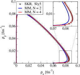
Figure 1: (Main plot) The thermodynamical spinodal for the Skyrme Sly5 model. SKR stands for the original Sly5 model spinodal while MM marks the spinodals calculated in the MM framework, for $N=2$ and $N=4$ cases. (Inserted plot) Enlarged neutron rich part of the spinodal where the CC transition point is to be found.

III.2 Low density correction parameter b

In previous studies using the meta-modeling method Margueron1 ; Margueron2 ; Chatterjee2017 the low density correction was defined fixing the $b$ parameter entering equation (7) as $b=\frac{n_{sat}}{n_{m}}ln(2)$, a quick vanishing of the correction being secured by $n_{m}$ being small but finite. We recall that the physical meaning of $n_{m}$ is the minimum density at which the Taylor expansion around saturation is considered to be valid. Since the correction term plays a role only at low densities, a constant choice for $b$ or equivalently $n_{m}$ will not influence the result when MM is applied to finite nuclei Chatterjee2017 or NSs Margueron2 as long as the value of $n_{m}$ is kept well below the saturation density. Nonetheless, the question is if this is true when we explore the sub-saturation region, in search for the crust-core phase transition point expected in the density range $0.05$ $fm^{-3}<n_{n}<0.09$ $fm^{-3}$ Ducoin:2011fy , and with $n_{p}$ an order of magnitude lower. It is therefore worthwhile to test the effect that a variation of the $b$ parameter will have on the spinodal shape for very asymmetric nuclear matter, where we expect to find the CCPT point. Several different values of $b$ parameter are given in the Table 1, as well as the corresponding density $n_{m}$ at which the low density correction is fixed.

Table 1: Change of the b parameter with $n_{m}$, the density at which the low density correction is fixed (see text).

$n_{m}$		$n_{m}[fm^{-3}]$		$b$
$0.075$ $n_{sat}$		$\sim 0.012$		$\sim 9.24$
$0.1$ $n_{sat}$		$\sim 0.016$		$\sim 6.93$
$0.2$ $n_{sat}$		$\sim 0.032$		$\sim 3.46$
$0.3$ $n_{sat}$		$\sim 0.048$		$\sim 2.31$
$0.4$ $n_{sat}$		$\sim 0.064$		$\sim 1.73$
$0.5$ $n_{sat}$		$\sim 0.08$		$\sim 1.38$
$0.6$ $n_{sat}$		$\sim 0.096$		$\sim 1.15$

The densities above $n_{m}>0.6$ $n_{sat}$ are not worthwhile to look at since we want to fix the low density correction well below saturation. The physically reasonable $n_{m}$ span the $b$ value over the range $1<b<10$. We can explore the effect that the change of the b parameter value has on the spinodal shape, while keeping in mind that the low density correction should be fixed at the density below the expected CC transition point density. This essentially means that the values of $b\leq 2$ can be excluded, since these values correspond to the densities $n>0.05$ $fm^{-3}$. The calculation of thermodynamical spinodal shapes is done within the MM approach for four different models (Sly5 CHABANAT1998231 , RATP RATP , SGII vanGiai:1981zz and LNS5 LNS5 ) and the result are compared with the exact spinodal, as given in Fig.2. The exact spinodal of the different models is marked with SKR while the spinodals calculated in the MM approach are marked with different $b$ values. The black line represents the stellar EOS whose crossing with spinodal gives the CC transition point density $n_{t}=n_{n,t}+n_{p,t}$.

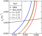
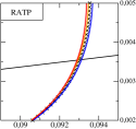
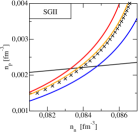
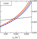
Figure 2: The influence of the low density correction parameter $b$ on the spinodal shape (for $N=4$) within the MM method for four different models (Sly5 CHABANAT1998231 , RATP RATP , SGII vanGiai:1981zz and LNS5 LNS5 ), compared to the original spinodal marked with SKR. See text for further details.

The best reproduction of the original models seems to be obtained for the $b$ value $b\sim 2.31$ in all four cases. While the variation of $b$ changes the spinodal shape by different rate for the four chosen interactions, the maximal change is of the order of $n_{t}\pm 0.001$ $fm^{-3}$ for all studied cases, which is one order of magnitude below the expected uncertainty on the CC point. Therefore, we can conclude that the variation of the $b$ parameter will certainly not give the dominant effect. It is important to point out that this is the consequence of including the higher order parameters ($N=3,4$) in the meta-model framework. When the expansion parameters in eq. (2) are taken only up to $N=2$, the change of the $b$ parameter in the low density region would cause more significant change of the CC density, of order $n_{t}\pm 0.01$ $fm^{-3}$. This is a first indication that higher order parameters, beyond the usually studied slope of the symmetry energy $L_{sym}$, must be considered.

IV Sensitivity study of thermodynamical and dynamical spinodals

The parameters of the MM approach are summarized as:

• empirical EOS parameters $\{P_{\alpha}\}\equiv\{n_{sat}$, $E_{sat}$, $K_{sat}$, $Q_{sat}$ $Z_{sat}$, $E_{sym}$, $L_{sym}$, $K_{sym}$, $Q_{sym}$, $Z_{sym}\}$;

• $\kappa_{sat}$ and $\kappa_{sym}$ that parametrize the isoscalar Landau effective mass $m^{\ast}$ as well as the proton-neutron mass splitting $\Delta m^{\ast}$;

• low density correction parameter $b$;

• for the case of dynamical spinodal, the isoscalar and isovector surface parameters $C_{fin}$ and $D_{fin}$ .

The question is how sensitive are the density and pressure of the phase transition point to the change of each of these parameters. To get an insight on this issue, two different reference parameter sets were used for the parameter sensitivity study of the LG and CC point, listed in table 2. The empirical EOS parameters $\{P_{\alpha}\}$ and the parameters $m^{\ast}$ and $\Delta m^{\ast}$ belonging to Set 1 in table 2 are obtained by averaging the single parameter value and its associated uncertainties over a total of 50 different Skyrme, RMF and RHF models, which all were successfully compared to experimental nuclear data. The low order (LO) parameters up to second order ($N=2$) are taken from table IV of reference Margueron1 . The higher order (HO) parameters ($N=3,4$) are taken from table VI of the same reference where HO parameters are better constrained in the MM approach by fixing the EOS at an additional reference point in density, $n_{0}=4n_{sat}$, besides the saturation density.

A second choice for a reference parameter set (Set 2 in table 2) is taken from table VII of Margueron1 and it contains LO parameters (up to $N=2$) extracted from experimental analysis, while the $Q_{sat,sym}$ and $Z_{sat,sym}$ are estimated from table VI, as for Set 1.

Table 2: The sets of empirical parameters and its associated uncertainties for the two EOS model reference points taken from reference Margueron1 . The additional parameters $b$, $C_{fin}$ and $D_{fin}$ are chosen or calculated (see text for details).

Parameter		$n_{sat}$	$E_{sat}$	$K_{sat}$	$Q_{sat}$	$Z_{sat}$	$E_{sym}$	$L_{sym}$	$K_{sym}$	$Q_{sym}$	$Z_{sym}$	$\frac{m^{\ast}}{m}$	$\frac{\Delta m^{\ast}}{m}$	$b$	$C_{fin}$	$D_{fin}$
set		$[\frac{1}{fm^{3}}]$	$[MeV]$	$[MeV]$	$[MeV]$	$[MeV]$	$[MeV]$	$[MeV]$	$[MeV]$	$[MeV]$	$[MeV]$			$[MeV]$	$[\frac{MeV}{fm^{5}}]$	$[\frac{MeV}{fm^{5}}]$
Set 1		$0.1543$	$-16.03$	$251$	$287$	$-1765$	$33.30$	$76.6$	$-3$	$-124$	$-437$	$0.72$	$0.01$	$2.31$	$52$	$-30$
$\sigma_{1}$		$0.0054$	$0.20$	$29$	$352$	$782$	$2.65$	$29.2$	$132$	$317$	$594$	$0.09$	$0.2$	$2$ and $10$	$52$	$30$
Set 2		$0.155$	$-15.8$	$230$	$300$	$-500$	$32$	$60$	$-100$	$0$	$-500$	$0.75$	$0.1$	$2.31$	$46$	$-70$
$\sigma_{2}$		$0.005$	$0.3$	$20$	$400$	$1000$	$2$	$15$	$100$	$400$	$1000$	$0.1$	$0.1$	$2$ and $10$	$46$	$70$

The average value for the $b$ parameter is taken to be $b=2.31$, the value that reproduces the four chosen model spinodals best. To study its sensitivity, this parameter is varied between the values of $2<b<10$, which matches the fact that the low density correction is fixed at a density between $0.01fm^{-3}<n_{0}<0.05fm^{-3}$.

The additional $C_{fin}$ and $D_{fin}$ parameters governing the surface properties of the energy functional are optimized for each EoS parameter set on experimental nuclear masses taken from the AME2012 mass table AME2012 .

Given a set of empirical parameters, the binding energies of several symmetric spherical nuclei (${}^{40}Ca$, ${}^{48}Ca$, ${}^{48}Ni$, ${}^{58}Ni$, ${}^{88}Sr$, ${}^{90}Zr$, ${}^{114}Sn$, ${}^{132}Sn$, ${}^{208}Pb$) are calculated in the extended Thomas Fermi (ETF) approximation using the parametrized density profiles of Ref. Aymard2014 . $C_{fin}$ and $D_{fin}$ are obtained from the following chi-square minimization:

$$\chi^{2}=\sum^{N}_{i=1}(E_{i,th}-E_{i,exp})^{2}/E_{i,exp}^{2}.$$ (25)

The optimal values, $C^{(opt)}_{fin}$ and $D^{(opt)}_{fin}$, for Set 1 and Set 2 that give minimal $\chi^{2}$ are given in table 2, with the $C_{fin}$ value being close to the previously found result for a study of finite nuclei Chatterjee2017 .

To study the sensitivity of the CC point to the finite size parameters, a physical interval has to be specified reflecting the uncertainty around the optimized value. An estimation for this interval can be obtained if we consider that the dynamical spinodal (corresponding to finite values for $C_{fin}$,$D_{fin}$) is always enveloped by the thermodynamical one (corresponding to $C_{fin}$=$D_{fin}=0$) . Imposing this condition gives the approximate ranges of the parameters $0\lesssim C_{fin}\lesssim 100$ and $0\lesssim D_{fin}\lesssim-150$, as given in table 2.

At this point, once we have the full sets of parameters ($\{P_{\alpha}\},m^{\ast},\Delta m^{\ast},b,C_{fin},D_{fin}$) according to set 1 and set 2, we find the thermodynamical (dynamical) spinodal of the system and, by finding the crossing between the spinodal and the $\beta$-equilibrated EOS, obtain the LG (CC) transition point density $n_{t}$ and pressure $P_{t}$. Further, by changing each of the parameter values individually by associated uncertainty $\pm\sigma$ we get an idea of the transition point sensitivity to each of the parameters individually. This sensitivity study is enveloped in Figure 3 for the thermodynamical spinodal and in Figure 4 for the dynamical one. For both figures, the top panels give the sensitivity of the density $n_{t}$ while the bottom ones represent the sensitivity of pressure $P_{t}$. The two dashed lines represent the transition value (in density or pressure) for the given sets from table 2, Set 1 being marked by circles and Set 2 by squares. Set 2, representing the parameter values constrained by experiment, gives slightly higher values for both transition density and pressure. There are three points depicted for each parameter of the two sets: the average value, which sits on the dashed line, and the two average $\pm\sigma$ values in addition.

In both cases, from the range of values for each of the parameters, we observe that the parameters $L_{sym}$ and $K_{sym}$ have the highest influence on LG and CC points both in transition density and pressure. If the influence of $L_{sym}$ was already reported in previous studies Ducoin:2011fy , the effect of $K_{sym}$ is less known. The reader should keep in mind that the very wide bands, as e.g. for $L_{sym}$ parameter for Set 1, are given by the average and uncertainty of $L_{sym}$ over 50 different models which therefore results in very wide range of values, $47.4<L_{sym}<105.8$. In contrast to that, the values from Set 2, extracted from dedicated experimental studies, are more restrictive, being $L_{sym}=60\pm 15$. The same goes for all the parameters.

It is also interesting to observe the very high sensitivity of the CC point to the low density parameter $b$. Even if the range for this parameter has been fixed in a largely arbitrary way and the functional form for the low density correction is also largely arbitrary, the observed sensitivity reflects the fact that the transition point depends on the properties of the functional in the very low density region, where the Taylor expansion breaks down because higher order correlation beyond the mean field might affect the the functional form beyond the derivatives at the saturation point.

Table 3: The phase transition density and pressure of different reference models (Set 1 and Set 2) for the LGPT and CCPT cases.

		$n_{t}$				$P_{t}$
		LGPT		CCPT		LGPT		CCPT
Set 1		$0.0637$		$0.0570$		$0.2472$		$0.1867$
Set 2		$0.0672$		$0.0587$		$0.3309$		$0.2442$

The transition points obtained for the two cases are given in table 3. As expected, when finite-size density fluctuations are included, the transition point is found at somewhat lower density and pressure.

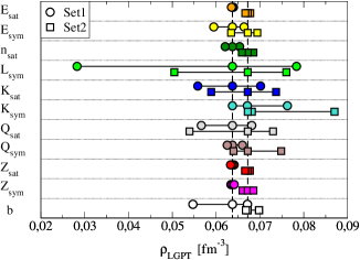
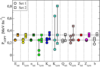
Figure 3: Sensitivity parameter study of the LG phase transition (LGPT) point for two reference points with parameters sets Set 1 and Set 2 (table (2)) taken from Ref. Margueron1 . The plots represent the sensitivity of transition density $n_{t}$ (Top) and pressure $P_{t}$ (Bottom) on the change of parameter values for $av\pm\sigma$.

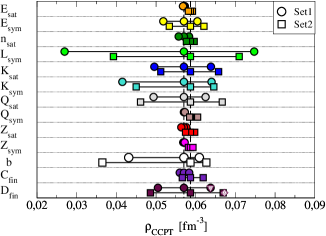
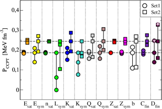
Figure 4: Same as Fig. 3 but for the CC phase transition (CCPT) point. Two additional parameters that come into play, $C_{fin}$ and $D_{fin}$, describe the surface properties of the functionals.

V Bayesian analysis of the dynamical spinodal CCPT point

In the next step, we restrict ourselves to the dynamical spinodal which represents more accurately the real transition point, and fully explore the parameter space of the meta-modeling, up to fourth order in Taylor expansion ($N=4$), within a Bayesian analysis. The prior is defined as a flat distribution of each of the parameters $(\vec{X})=(\{P_{\alpha}\},m^{\ast},\Delta m^{\ast},b)$, with a parameter values interval given in table 4.

The posterior distribution is obtained by applying two different physical filters to the prior distribution,

$$p_{post}(\vec{X})=\mathpzc{N}\,w(\vec{X})\,e^{-\chi^{2}(\vec{X})/2}\,p_{prior}(\vec{X}).$$ (26)

In this expression, both strict ($w$ term) and likelihood (exponential term) filters are applied, and $\mathpzc{N}$ is a normalization. $\chi^{2}(\vec{X})$ represents the $\chi^{2}$ corresponding to the optimal fit of nuclear masses which is done to determine the surface tension parameters $C_{fin}$ and $D_{fin}$ for each $\vec{X}$ parameter set (see section IV). $w$ is a sharp $\delta$-function filter that outputs 1 if the constraint is respected, and 0 otherwise. The constraint consists in requiring that each model lays within the uncertainty band of the N3LO effective field theory calculation of energy and pressure for SM and pure neutron matter (PNM) of Ref. Drischler2016 in the density interval $0.05fm^{-3}<n<0.2fm^{-3}$.

In this global bayesian determination of the uncertainty intervals for the a-priori independent model parameters, the determination procedure of $C_{fin}(\vec{X})$ and $D_{fin}(\vec{X})$ by $\chi^{2}$ minimization can be only justified if the $\chi^{2}$ minimum is sufficiently shallow to consider that any other value for $C_{fin}$, $D_{fin}$ would be filtered out once the likelihood constraint on nuclear masses is applied.

To explore this issue, we consider the distribution of $\chi^{2}$ value around minimum for two representative reference models, shown in Figure 5. The behavior is qualitatively similar for all meta-modeling parameter sets.

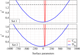
Figure 5: The $\chi^{2}$ minimum for $C_{fin}$ and $D{fin}$ parameters for the two reference point models.

We can see that the $D_{fin}$ minimum is very flat, reflecting the fact that stable nuclei very poorly constrain the isovector gradient terms. For that reason, we enlarge our prior distribution by associating to each parameter set $(\vec{X})$ two extra possible combinations of the surface parameters, which span the uncertainty of the $\chi^{2}$ minimum. Specifically, we impose a condition on $\chi^{2}$ that the ratio of maximal and minimal probabilities is $P_{min}/P_{max}=1/2$ where $P_{max,min}$ $\propto$ $\exp^{-\chi^{2}_{min,max}/2}$. The condition is then

$$\chi^{2}_{max}=2ln(2)+\chi^{2}_{min},$$ (27)

given by the dashed line in the Figure 5. The crossings between the $\chi^{2}_{max}$ and the $C_{fin}$ and $D_{fin}$ lines gives the minimum and maximum values which can be adopted for the surface parameters. This procedure gives a more realistic estimation of the uncertainty associated to the surface parameters, with respect to the rough and extreme condition of Section IV that the dynamical spinodal must be embedded into the thermodynamical one. Still, this $\chi^{2}$ criterium implies that $C_{fin}$ and $D_{fin}$ are independent, which is certainly not the case. The large range in $D_{fin}\pm\sigma$ can be further reduced by looking which $D_{fin}$ values actually represent physical solutions. We have found that the very negative values of $D_{fin}$ are not physical by imposing the condition that the combined effect of surface and Coulomb terms in eq. (21) should quench the thermodynamical instability (i.e. $k\rightarrow 0$), and not amplify it. This condition can be expressed as

$$\lim_{k\rightarrow 0}e_{2}(\mathcal{C}_{k})=0^{+}$$ (28)

where $e_{2}(\mathcal{C}_{k})$ is the lowest eigenvalue of the reduced matrix

$$\mathcal{C}_{k}=k^{2}\mathcal{C}_{surf}+\frac{\alpha}{k^{2}}\mathcal{C}_{Coul}.$$ (29)

Since the electrons play negligible role in the finite size spinodal Ducoin2007 , we can impose this condition to the nuclear matter without electrons, that is

$$\mathcal{C}_{k}=\begin{pmatrix}(C_{fin}+D_{fin})k^{2}&(C_{fin}-D_{fin})k^{2}&0\\ (C_{fin}-D_{fin})k^{2}&(C_{fin}+D_{fin})k^{2}&\frac{\alpha}{k^{2}}.\\ \end{pmatrix}$$ (30)

The eigenvalues $e$ of this matrix are

$$2e=\operatorname{Tr}{(\mathcal{C}_{k})}\pm\sqrt{\operatorname{Tr}^{2}{(\mathcal{C}_{k})}-4\det{(\mathcal{C}_{k}})}$$ (31)

which, after applying the condition (28), restricts the minimal value of $D_{fin}$ parameter to the value

$$D_{fin}^{(min)}=-C^{(opt)}_{fin}.$$ (32)

Summarizing the discussion, each parameter set $(\vec{X})=(\{P_{\alpha}\},m^{\ast},\Delta m^{\ast},b)$ of our prior distribution will be associated to three different parameter sets, namely

• $\vec{X},C_{fin}=C^{(opt)}_{fin},D_{fin}=D1=-C^{(opt)}_{fin}$,

• $\vec{X},C_{fin}=C^{(opt)}_{fin},D_{fin}=D3=D^{opt}_{fin}+\sigma$,

• $\vec{X},C_{fin}=C^{(opt)}_{fin},D_{fin}=D2=(D1+D2)/2$.

The so-defined prior set has been run through the filter given by the low density ab-initio calculation (LD) and the mass reproduction filter eq.(26). Our posterior set is constituted of 5412 models. It is interesting to remark that the low density filter Drischler2016 is much more constraining than the mass filter. Applying this latter after the LD filter does not give any significant changes in the parameter expectation values and variances. Still the mass filter allows determining reliable values of the two gradient couplings, $C_{fin}$ and $D_{fin}$ which enter in the spinodal determination.

Table 4: The prior and posterior average values and variances.

				$n_{sat}$	$E_{sat}$	$K_{sat}$	$Q_{sat}$	$Z_{sat}$	$E_{sym}$	$L_{sym}$	$K_{sym}$	$Q_{sym}$	$Z_{sym}$	$\frac{m^{\ast}}{m}$	$\frac{\Delta m^{\ast}}{m}$	$b$	$C_{fin}$	$D_{fin}$
				$[\frac{1}{fm^{3}}]$	$[MeV]$	$[MeV]$	$[MeV]$	$[MeV]$	$[MeV]$	$[MeV]$	$[MeV]$	$[MeV]$	$[MeV]$			$[MeV]$	$[\frac{MeV}{fm^{5}}]$	$[\frac{MeV}{fm^{5}}]$
Prior		Av		$0.16$	$-16$	$230$	$0$	$0$	$32$	$45$	$-100$	$0$	$0$	$0.7$	$0.1$	$5.5$
		$\sigma$		$0.01$	$1$	$40$	$1000$	$3000$	$6$	$35$	$300$	$2000$	$5000$	$0.1$	$0.1$	$4.5$
LD		Av		$0.164$	$-15.29$	$234$	$-31$	$-146$	$30.7$	$43.7$	$-202$	$-253$	$-114$	$0.70$	$0.10$	$5.2$	$30$	$115$
+ mass filter		$\sigma$		$0.005$	$0.25$	$23$	$362$	$1728$	$0.8$	$3.7$	$42$	$673$	$2868$	$0.06$	$0.06$	$2.6$	$9$	$143$

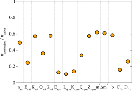
Figure 6: The representation of the parameter restrictions imposed by LD and mass filter and compared to the initially defined prior.

Figure 6 presents the variance reduction after the LD and mass filter in each of the parameters, as given in table 4. It is represented as the ratio of the posterior and prior variances for each of the model parameters. In this representation, the parameters with small value of the ratio are significantly constrained through the LD filtering method compared to the prior range. As seen in Figure 6, the filtering procedure is very constraining for all parameters except the fourth order derivatives ($Z_{sat}$ and $Z_{sym}$), which in any case are not strongly influential in the determination of the CC point (see Section IV). The reduced impact on quantities like $K_{sat}$, $n_{sat}$ and $m^{\ast}$ can be understood from the fact that our prior distribution from table 4 takes into account the actual present knowledge of the different parameters from nuclear physics experiments. The quantities $K_{sat}$, $n_{sat}$ and $m^{\ast}$ are already very well constrained, meaning that their prior dispersion is already very small, which explains the reduced effect of the filter.

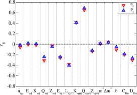
Figure 7: The correlation indices values $r_{ij}$ between the model parameters ($i$) and the CC transition point density $n_{t}$ and pressure $P_{t}$ ($j$).

Finally, the question we want to address is how much the CC point is correlated to the model parameters. The values of correlation indexes $r_{ij}$, where $i=n_{t}$, $P_{t}$ and $j=\{P_{\alpha}\}$, $m^{\ast}/m$, $\Delta m^{\ast}/m$, $b$, $C_{fin}$, $D_{fin}$, are given in Figure 7. The well determined LO parameters have, as usually found, very little influence on the CC point. However, along with the expected strong correlation with the $L_{sym}$ parameter, the $n_{t}$ and $P_{t}$ show also a significant correlation with the isovector curvature $K_{sym}$ as well as with the $N=3$ order parameters, especially with $Q_{sym}$. This is in good qualitative agreement with the findings of the sensitivity analysis in Section IV. We can also see that the important role on the transition point played by the behavior at very low density, as expressed by the influence of the $b$ parameter in Section IV, is strongly reduced in the correlation matrix. This can be understood from the important constraint at very low density given by the EFT calculations (LD filter).

VI Conclusion

The influence of the uncertainties in the EOS parameters on the crust-core phase transition (CCPT) point was explored within a meta-modeling (MM) approach. We have shown that at such low densities, the MM approach has to go beyond the second order expansion of energy per particle and take the higher orders into account in order to accurately reproduce the spinodal shapes of reference models. This underlines the important influence of high order empirical parameters beyond the symmetry energy at saturation $E_{sym}$ and its slope $L_{sym}$, on the properties of the transition. This is evident from the obtained high correlation index between the CC density and pressure values and the $N=2,3$ isovector empirical EOS parameters, as in Figure 7.

A quantitative estimation of the model dependence on the transition point was obtained through a complete Bayesian analysis of the EoS parameters, where the multi-dimensional EoS parameter space has been constrained to reproduce the low density N3LO effective field theory predictions of Ref. Drischler2016 , and the gradient couplings have been constrained to reproduce experimental nuclear masses.

Our final predictions for the CC transition density and pressure are $n_{t}=(0.071\pm 0.011)$ $fm^{-3}$ and $P_{t}=(0.294\pm 0.102)$ $MeVfm^{-3}$, respectively.

It might be disappointing to remark that the obtained uncertainty on the transition point is not much different from the present dispersion coming from compilations of phenomenological relativistic and non-relativistic models (see for instance Ducoin:2011fy ), in spite of the fact that all used MMs satisfy the ab-initio constraints, which are very restrictive at low density. The reason for this is possibly the fact that the reduced interval of $L_{sym}$ implied by the ab-initio filter with respect to the range of popular models, is compensated by wider uncertainty in the isovector high order and surface parameters. Improved predictions thus will require further experimental constraints for very low density asymmetric matter, such as for e.g. measurement of neutron skins Boso2018 .

References

- [1] Francois Aymard, Francesca Gulminelli, and Jérôme Margueron. In-medium nuclear cluster energies within the extended thomas-fermi approach. Phys. Rev. C, 89:065807, Jun 2014.
- [2] Slavko Bogdanov. The Nearest Millisecond Pulsar Revisited with XMM-Newton: Improved Mass-Radius Constraints for PSR J0437-4715. Astrophys. J., 762:96, 2013.
- [3] A. Boso, S. M. Lenzi, F. Recchia, J. Bonnard, A. P. Zuker, S. Aydin, M. A. Bentley, B. Cederwall, E. Clement, G. de France, A. Di Nitto, A. Dijon, M. Doncel, F. Ghazi-Moradi, A. Gadea, A. Gottardo, T. Henry, T. Hüyük, G. Jaworski, P. R. John, K. Juhász, I. Kuti, B. Melon, D. Mengoni, C. Michelagnoli, V. Modamio, D. R. Napoli, B. M. Nyakó, J. Nyberg, M. Palacz, J. Timár, and J. J. Valiente-Dobón. Neutron skin effects in mirror energy differences: The case of . Phys. Rev. Lett., 121:032502, Jul 2018.
- [4] Bao-Jun Cai and Lie-Wen Chen. Nuclear matter fourth-order symmetry energy in the relativistic mean field models. Phys. Rev., C85:024302, 2012.
- [5] L. G. Cao, U. Lombardo, C. W. Shen, and Nguyen Van Giai. From brueckner approach to skyrme-type energy density functional. Phys. Rev. C, 73:014313, Jan 2006.
- [6] E. Chabanat, P. Bonche, P. Haensel, J. Meyer, and R. Schaeffer. A skyrme parametrization from subnuclear to neutron star densities part ii. nuclei far from stabilities. Nuclear Physics A, 635(1):231 – 256, 1998.
- [7] D. Chatterjee, F. Gulminelli, Ad. R. Raduta, and J. Margueron. Constraints on the nuclear equation of state from nuclear masses and radii in a thomas-fermi meta-modeling approach. Phys. Rev. C, 96:065805, Dec 2017.
- [8] C. Drischler, K. Hebeler, and A. Schwenk. Asymmetric nuclear matter based on chiral two- and three-nucleon interactions. Phys. Rev. C, 93:054314, May 2016.
- [9] C. Ducoin, Ph. Chomaz, and F. Gulminelli. Isospin-dependent clusterization of neutron-star matter. Nuclear Physics A, 789(1):403 – 425, 2007.
- [10] C. Ducoin, J. Margueron, and C. Providência. Nuclear symmetry energy and core-crust transition in neutron stars: A critical study. EPL (Europhysics Letters), 91(3):32001, 2010.
- [11] Camille Ducoin, Jerome Margueron, Constanca Providência, and Isaac Vidaña. Core-crust transition in neutron stars: predictivity of density developments. Phys. Rev., C83:045810, 2011.
- [12] M. Dutra, O. Lourenco, J. S. Sa Martins, A. Delfino, J. R. Stone, and P. D. Stevenson. Skyrme interaction and nuclear matter constraints. Phys. Rev. C, 85:035201, Mar 2012.
- [13] F. J. Fattoyev and J. Piekarewicz. Sensitivity of the Moment of Inertia of Neutron Stars to the Equation of State of Neutron-Rich Matter. Phys. Rev., C82:025810, 2010.
- [14] C. Gonzalez-Boquera, M. Centelles, X. Vinas, and A. Rios. Higher-order symmetry energy and neutron star core-crust transition with Gogny forces. Phys. Rev., C96(6):065806, 2017.
- [15] Brynmor Haskell and Andrew Melatos. Models of pulsar glitches. Int. J. Mod. Phys. D, 24:1530008, 2015.
- [16] C. J. Horowitz and J. Piekarewicz. Neutron star structure and the neutron radius of . Phys. Rev. Lett., 86:5647–5650, Jun 2001.
- [17] Takashi Okajima Keith C. Gendreau, Zaven Arzoumanian. The neutron star interior composition explorer (nicer): an explorer mission of opportunity for soft x-ray timing spectroscopy. Proc.SPIE, 8443, 2012.
- [18] T. Klähn, D. Blaschke, S. Typel, E. N. E. van Dalen, A. Faessler, C. Fuchs, T. Gaitanos, H. Grigorian, A. Ho, E. E. Kolomeitsev, M. C. Miller, G. Röpke, J. Trümper, D. N. Voskresensky, F. Weber, and H. H. Wolter. Constraints on the high-density nuclear equation of state from the phenomenology of compact stars and heavy-ion collisions. Phys. Rev. C, 74:035802, Sep 2006.
- [19] A. Li, J. M. Dong, J. B. Wang, and R. X. Xu. Structures of the Vela pulsar and the glitch crisis from the Brueckner theory. Astrophys. J. Suppl., 223(1):16, 2016.
- [20] Bennett Link, Richard I. Epstein, and James M. Lattimer. Pulsar constraints on neutron star structure and equation of state. Phys. Rev. Lett., 83:3362–3365, Oct 1999.
- [21] Jerome Margueron, Rudiney Hoffmann Casali, and Francesca Gulminelli. Equation of state for dense nucleonic matter from metamodeling. i. foundational aspects. Phys. Rev. C, 97:025805, Feb 2018.
- [22] Jerome Margueron, Rudiney Hoffmann Casali, and Francesca Gulminelli. Equation of state for dense nucleonic matter from metamodeling. ii. predictions for neutron star properties. Phys. Rev. C, 97:025806, Feb 2018.
- [23] Ch. C. Moustakidis, T. Niksic, G. A. Lalazissis, D. Vretenar, and P. Ring. Constraints on the inner edge of neutron star crusts from relativistic nuclear energy density functionals. Phys. Rev., C81:065803, 2010.
- [24] M. Oertel, M. Hempel, T. Klahn, and S. Typel. Equations of state for supernovae and compact stars. Rev. Mod. Phys., 89(1):015007, 2017.
- [25] H. Pais, A. Sulaksono, B. K. Agrawal, and C. Providência. Correlation of the neutron star crust-core properties with the slope of the symmetry energy and the lead skin thickness. Phys. Rev., C93(4):045802, 2016.
- [26] C.J. Pethick, D.G. Ravenhall, and C.P. Lorenz. The inner boundary of a neutron-star crust. Nuclear Physics A, 584(4):675 – 703, 1995.
- [27] G. Audi;M. Wang;;A.H. Wapstra;F.G. Kondev;M. MacCormick;X. Xu;B. Pfeiffer. The ame2012 atomic mass evaluation (i). evaluation of input data, adjustment procedures. Chinese physics C, 36(12):1287, 2012.
- [28] J. Piekarewicz and M. Centelles. Incompressibility of neutron-rich matter. Phys. Rev. C, 79:054311, May 2009.
- [29] M. Rayet, M. Arnould, G. Paulus, and F. Tondeur. Nuclear forces and the properties of matter at high temperature and density. Astron.Astrophys., 116:183–187, 1982.
- [30] T. R. Routray, X. Vinas, D. N. Basu, S. P. Pattnaik, M. Centelles, L. Robledo, and B. Behera. Exact versus Taylor-expanded energy density in the study of the neutron star crust–core transition. J. Phys., G43(10):105101, 2016.
- [31] A. W. Steiner, S. Gandolfi, F. J. Fattoyev, and W. G. Newton. Using neutron star observations to determine crust thicknesses, moments of inertia, and tidal deformabilities. Phys. Rev. C, 91:015804, Jan 2015.
- [32] Nguyen van Giai and H. Sagawa. Spin-isospin and pairing properties of modified Skyrme interactions. Phys. Lett., 106B:379–382, 1981.
- [33] Isaac Vidaña, Constanca Providência, Artur Polls, and Arnau Rios. Density dependence of the nuclear symmetry energy: A Microscopic perspective. Phys. Rev., C80:045806, 2009.
- [34] Anna L. Watts, Nils Andersson, Deepto Chakrabarty, Marco Feroci, Kai Hebeler, Gianluca Israel, Frederick K. Lamb, M. Coleman Miller, Sharon Morsink, Feryal Özel, Alessandro Patruno, Juri Poutanen, Dimitrios Psaltis, Achim Schwenk, Andrew W. Steiner, Luigi Stella, Laura Tolos, and Michiel van der Klis. Colloquium: Measuring the neutron star equation of state using x-ray timing. Rev. Mod. Phys., 88:021001, Apr 2016.