Berezinskii-Kosterlitz-Thouless transition on regular and Villain types of -state clock models
Abstract
We study -state clock models of regular and Villain types with using cluster-spin updates and observed double transitions in each model. We calculate the correlation ratio and size-dependent correlation length as quantities for characterizing the existence of Berezinskii-Kosterlitz-Thouless (BKT) phase and its transitions by large-scale Monte Carlo simulations. We discuss the advantage of correlation ratio in comparison to other commonly used quantities in probing BKT transition. Using finite size scaling of BKT type transition, we estimate transition temperatures and corresponding exponents. The comparison between the results from both types revealed that the existing transitions belong to BKT universality.
1 Introduction
The two-dimensional (2D) -state clock models play an important role in the study of phase transitions as they provide links between several seminal works [1, 2, 3, 4, 5]. The underline symmetry is a generalization of Ising model, the most studied and the first model in statistical physics found to exhibit a phase transition [1]. The XY model, their continuous counterpart, is the native host of a unique phase which is the only type of order allowed by the well known Mermin-Wagner theorem [2] for a 2D pure system with continuous symmetry. It is a quasi-long-range order (QLRO) called Berezinskii-Kosterlitz-Thouless (BKT) phase [3, 4, 5]; essentially a topological excitation state in the form of vortex-antivortex pairs. The BKT phase is ubiquitous for many system, observed for example in a planar array of coupled Josephson junctions in transverse magnetic field [6, 7], liquid crystal [8] and the low-dimensional ferroelectrics [9]. Interestingly, this type of phase is inherited by the clock models, depending on the parameter which evenly divides into equal angles.
Based on the Mermin-Wagner theorem above mentioned, a discrete symmetry is important for the existence of a true LRO in 2D systems. It was theoretically predicted [10, 11] and later confirmed numerically by several early studies [12, 13, 14] that the -state clock models experience two transitions for , i.e., the lower () and the higher temperature () transitions, where the BKT phase exists between them. The typical characteristics of this phase is related to the existence of vortex-antivortex formation. Mathematically, this exotic pattern is associated with the power-law behavior of the spin-spin correlation function. Since it is not possible to obtain such a formation out of spins with symmetry for , the corresponding models cannot host a BKT phase. A relatively small excitation is not allowed as any possible change of angular directions is always large. This leads the low-temperature excitation to be occupied by a true LRO, rather than BKT phase. For there is an interplay between the discreteness which tends to create an LRO at low temperature and the inherited symmetry trying to preserve BKT phase. The conformity of both causes the LRO to exist below the BKT phase. Thereby two transition temperatures, , are observed; each corresponds to transition between LRO and QLRO and between QLRO and a disordered phase. The LRO is induced by the discrete symmetry of the clock model.
In recent years, the study of phase transition of -state clock models has regained a lot of interest, in particular to probe whether the existing double transitions are BKT-type or not [15, 16, 17, 18, 20, 21, 19]. Analytical results from a related model called Villain model [22] revealed that both transitions are BKT type and interconnected via duality relation [10] for . Although such relation does not exist in the regular clock models, the renormalization group study [11] as well as standard Monte Carlo studies [12, 23] pointed out two separate transitions belonging to BKT universality. This is in contrast to the report by Lapilli et al. [15] who suggested that the transitions are BKT type only for . A study based on Fisher zero approach claimed that the transitions for are not BKT type [16], which could possibly be an artifact result from small system sizes [17]. While observing double transition for , Baek et al. [18, 19] concluded that transitions are BKT type for , but not for due to the role played by the supposed residual symmetry . However, more recent study by Kumano et al. [20] and Chatelain [21] are in favor of the previous scenario that the two transitions belonging to BKT type. With these conflicting results, the controversy on the type of phase transitions of -state clock models is mainly related to . Further investigation using different approaches is required, primarily to study -state clock models for .
In this paper, we report our study on these particular models, and try to address the controversy. We perform numerical study on regular (cosine) and Villain types of the models. The Villain type is quite interesting due to the existence of exact dual transformation by which the lower and higher temperature transitions are exchangeable. Due to the similarity of the underlining symmetry with the clock models, studying Villain model can bring a clear insight related to the debated issue; in particular if one uses the correlation ratio in characterizing the BKT transition. We argue that this quantity is more straightforward and exceptionally suitable in capturing the pattern of vortex-antivortex binding.
The remaining part of the paper is organized as follows: Section II describes the models and the method. The results are discussed in Section III while Section IV is devoted to the concluding remarks. Supplementary subjects are discussed in Appendices.
2 Models and Simulation Method
A -state clock model of regular (cosine) type is defined by the following Hamiltonian
| (1) |
where spins on lattice sites are planar spins restricted to align in discrete angles ( with ). The sum is over nearest-neighbor sites of square lattice (), with periodic boundary conditions. The interaction is ferromagnetic () by which all spins are aligned in the ground state configuration with -fold degeneracy; the ground state energy is for the square lattice.
By rewriting Eq. (1) as with , we can assign a local Boltzmann factor for the clock model as , where with as the inverse temperature. Villain type of clock model is obtained by introducing a set of auxiliary fields [10, 22]. For the Villain model, the local Boltzmann factor is given by
| (2) |
The result of the summation of Gaussian function in Eq. (2) over yields a similar form to the local Boltzmann factor of the clock model. The energy origin had better be shifted as for comparison. As we consider the regular (cosine) and Villain types of the models for , there are four models altogether.
For a reliable calculation, we use the canonical Monte Carlo method with cluster spin updates proposed by Swendsen and Wang [24] and adopt the embedded scheme of Wolff [25] in constructing a cluster for clock spins. A cluster spin algorithm is crucial for Monte Carlo study in order to avoid drawback of single spin update which is frequently suffering from slowing down near the critical point. This is done by projecting the spins into a randomly selected orientation, out of possibilities, so that the spins are divided into two groups (Ising-like spins). The embedded scheme is essential in carrying out cluster algorithm for such multi-component spins as planar and Heisenberg spins. After the projection, the original step of the cluster algorithm is performed, i.e., by connecting the spin to its nearest neighbors of the same group, with suitable probability depending on the local Boltzmann factor [26]. Spins in the cluster are updated at a time. One Monte Carlo step (MCS) is defined as updating all the spins.
We make measurement for the systems of linear size up to . In the careful discussion on the helicity modulus, which will be given in Appendix A, we treat large enough sizes up to . For the calculation of large systems, we use the GPU-based algorithm for the Swendsen-Wang algorithm [27], which is efficient for high-performance computing. Measurement is performed after enough equilibration steps ( MCS’s). Each data point is obtained from the average over several parallel runs, with MCS’s for each run. Typically, 5 measurements are done for each system size in order to estimate statistical errors. This means, each data point is obtained from the average of samples.
3 Results
3.1 BKT transitions and Correlation ratio
A BKT phase is essentially a topological excitation in the form of vortex-antivortex pairs [4, 5]. In the case of XY model, the unbinding of these pairs at high temperature is assigned as BKT transition which separates the BKT phase and paramagnetic phase. It corresponds to the transition of the clock models which have additional lower-temperature () transition. The disappearance of vortex-antivortex pairs following the unbinding scenario at high temperatures is associated with the vanishing of helicity modulus [28, 29]. We briefly discuss this quantity in Appendix A and present the result for examining the existing BKT phase of the 5-state and the 6-state clock model. Although this quantity is commonly used to probe BKT transition, it is not quite precise in characterizing the transition as the disappearance of vortex-antivortex pairs at low temperature follows different mechanism. In the case of the clock model, the spin-wave excitations are prohibited due to the energy gap of discrete models at low temperatures. Thus, the vortex-antivortex pairs disappear at low temperatures, associated with the transition; although the origin of this transition is due the discrete symmetry of the clock models. The conflicting main conclusions reported by Refs. [18, 19] and Refs. [21] suggest a more accurate way of calculating the helicity modulus when dealing BKT transitions of the clock models [20].
A quantity called correlation ratio [30] is particularly applicable to probing BKT transitions both for the upper and the lower transitions, and has been used in various cases [31, 32, 33]. It is a ratio of correlation functions with different distances. At a critical point or line (BKT phase), the correlation function for an infinite system decays as a power of distance ,
| (3) |
where and are respectively the lattice dimension and decay exponent. The angular bracket denotes the thermal average. It incorporates two length ratios for a finite system of linear system size away from the critical point or line,
| (4) |
with a correlation length for the infinite system. The ratio of correlation functions of different distances,
| (5) |
will have a single scaling variable for finite size scaling (FSS),
| (6) |
if we fix two ratios and . In principle, one can take any pair of distances, but for the convenience of numerical calculation we choose and .
At the critical region, where the correlation length is infinite, the correlation ratio, Eq. (6), does not depend on the system size . Thus, it is natural to expect a presence of a crossing point for the existence of a continuous transition or collapsing curves for that of BKT phase in the plot of temperature dependence of correlation ratio for different system sizes.
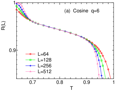
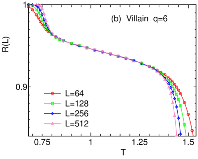
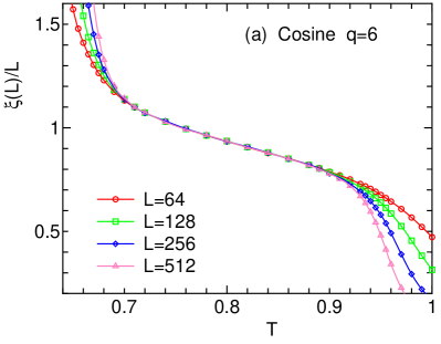
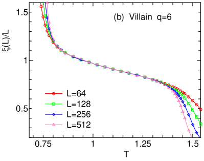
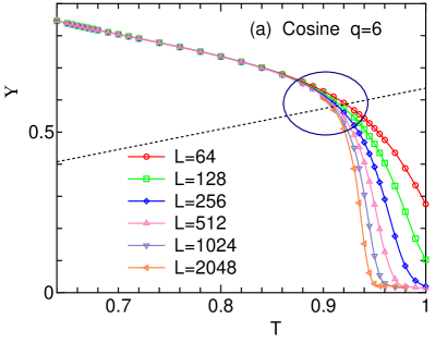
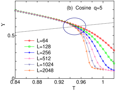
We plot, as shown in Fig. 1, the temperature dependence of the correlation ratio,
| (7) |
for of (a) regular and (b) Villain types, respectively. The plots have three typical temperature regimes, i.e., the lower, the intermediate and the upper regime. Each is associated with LRO, the BKT phase and the paramagnetic phase. The BKT phase is indicated by the collapsing curves of different system sizes. It is a direct consequence of power law behavior of correlation function at BKT phase. The spray out of the curves at lower and higher temperatures signifies two separated transitions.
The overall behavior of the correlation ratio, depicted in Fig. 1, is essentially the same for the model of regular type and that of Villain type. For the Villain model, the upper and the lower transitions are inter-connected via an exact duality relation [10],
| (8) |
and both transitions are BKT type [23]. Although there is not an exact duality relation for the regular clock model, quantitative data shown in Fig. 1 strongly suggest the universality of two transitions for regular and Villain types of clock model.
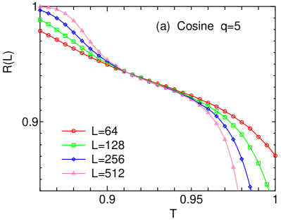
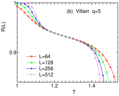
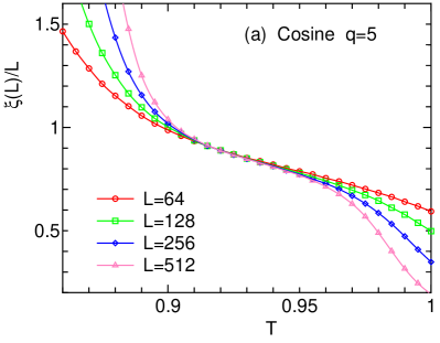
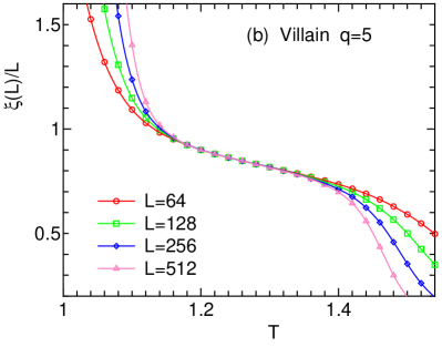
Analogous to Fig. 1, we plot the correlation ratio of (a) regular and (b) Villain types for in Fig. 2. The typical pattern of correlation ratio indicating the existence of BKT phase preserves, except that the collapsing regime becomes narrow, which indicates that the two transitions are getting closer. The discreteness suppresses the lower temperature excitation, but it does not totally rule out the BKT phase. Since the pattern of regular type is similar to that of Villain model, we argue that the transitions of 5-state clock model are also BKT type. The precise estimates of transition temperatures and the corresponding exponents are presented in the next sub-section.
The excellent performance of correlation ratio in characterizing the existence of BKT transition is related to the fact that it directly incorporates the correlation function, whose algebraic decay at BKT phase is a typical characteristic. We note that although the Binder ratio [34], essentially the moment ratio, has the same FSS property as in Eq. (6), the behavior of the collapsing and spraying out is not good due to the large corrections to FSS [30].
We also calculate the size-dependent 2nd-moment correlation length for finite system, , which is defined as[11]
| (9) |
with
| (10) |
The quantity has an FSS property similar to Eq. (6), and has been frequently used in spin glass problems [35]. In this case again, the FSS of the Binder ratio [34] is not good compared to that of .
We plot for the regular and Villain types of in Fig. 3. The collapsing curves at intermediate temperature regime and the spray out at lower and higher temperatures were observed at both types of models. This is another indication that the transitions of Villain and the regular types are of the same universality. For , shown in Fig. 4, the temperature range in which curves are collapsing becomes narrow; it is consistent with what observed for the correlation ratio shown in Fig. 2. All the data and plots presented thus far indicate that the transitions of -state clock models of both types for are universal.
3.2 FSS and the estimate of critical parameters
FSS is a standard technique in the study of phase transition. It is used to extract critical parameters from the finite system sizes. Here, we present FSS analysis based on diverging behavior of correlation length at BKT phase,
| (11) |
with . We choose and a constant such that all the data points in Fig. 4 are collapsed on a single curve for both the lower transition temperature () and the higher transition temperature ().
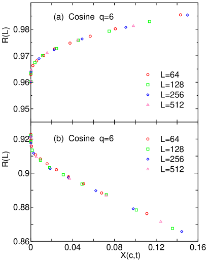
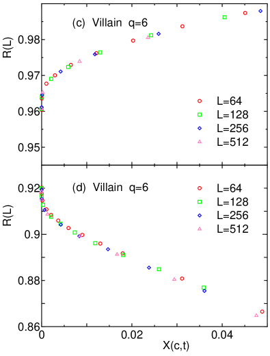
The FSS plot of the correlation ratio, whose original data is given in Fig. 1, is shown in Fig. 5, associated with the data for =6 of regular and Villain models. The plot is obtained by rescaling the horizontal axis, . The scaled variable is defined by
| (12) |
and are and for lower-temperature transition, and they are and for higher-temperature transition, and being the fitting parameters. Choosing several pairs of and as well as and , we obtained the fits for the estimated values. Our estimate for and for the regular model are respectively and ; while for the Villain model = and =. The numbers in parentheses are the uncertainty for the last digits. The transition temperatures for the Villain model are higher.
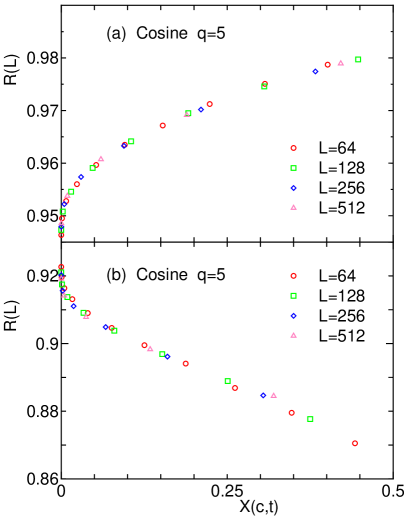
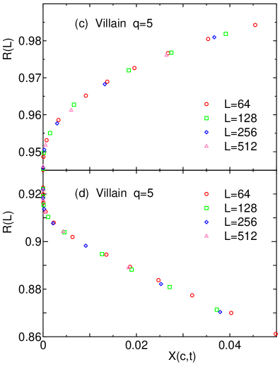
Similar procedure is applied to obtain plot shown in Fig. 6, which is the FSS plot of Fig. 2, associated with the data for regular and Villain model for =5. The estimates of and transition temperatures for regular model are respectively and . The two transitions are very close to each other in comparison to the transitions for of the same model. This is related to the role played by the discreteness which almost rules out the BKT phase. For the Villain model, the estimate for and are respectively and . Here, the temperature range is relatively wider compared to that of regular case.
The obtained set of transition temperatures, ’s and ’s, are tabulated in Table 1, where the duality relation (Eq. (8)) are checked for the Villain type. As indicated, the duality relation is verified, both for and , which indicates the accuracy of the present calculation.
| 6 (regular) | 0.120 | 0.236 | |||
| 5 (regular) | 0.176 | 0.234 | |||
| 6 (Villain) | 0.129 | 0.233 | |||
| 5 (Villain) | 0.176 | 0.235 |
3.3 FSS without estimating
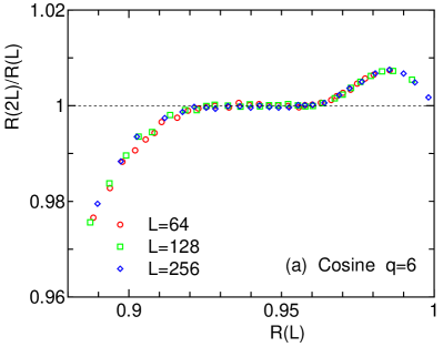
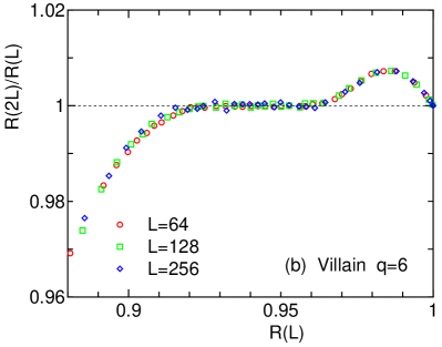
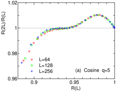
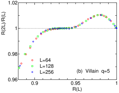
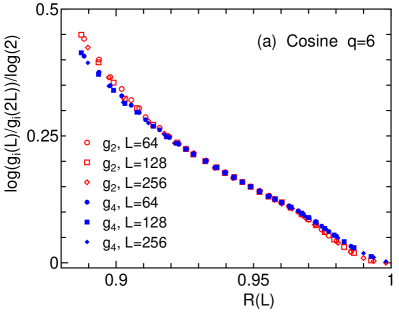
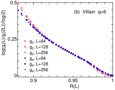
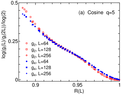
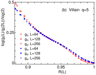
We here perform the FSS analysis without estimating to investigate the universality of the BKT transition. Such approach was recently employed in the study of the generalized XY model [36], where the analysis for the Potts model [37, 38] was applied to the study of the BKT transition. We focus on the FSS property of the ratio of the correlation ratio of different sizes, that is, .
We plot as a function of in Fig. 7 for four models, (a) regular and (b) Villain models for =6 and (c) regular and (d) Villain models for =5. The lattice size pairs - with =64, 128 and 256 are used. All the data for different sizes are collapsed on a single curve for each model. That is, the FSS is very good, although logarithmic corrections might not be small in the BKT transition [5, 39]. The value of remains 1 for the intermediate BKT phase, and becomes smaller than 1 for smaller , which means , as in the XY model [36]. The regime at which the collapsing curves are parallel to the horizontal axis with the value of 1 is equivalent to the collapsing regime of the plot in Fig. 1 and Fig. 2, the regime for the existence of BKT phase. For clock model of , the value of becomes larger than 1 for larger , that is, , and comes back to 1 for , that is, ; this behavior comes from the ordered phase.
We assign the values of at and as and , respectively. The values of and of regular model and Villain model are very close but there is a small difference for . For , the intermediate region becomes narrower, and the difference of regular and Villain models becomes more appreciable. The overall FSS behaviors of regular and Villain models look the same, but quantitatively two are not identical. This difference becomes larger for , because the difference of the local Boltzmann factor becomes larger for high temperatures.
The temperature dependence of decay exponent is extracted from the data of correlation function. This is done based on Eq. (4), , from which we obtain the following scaling form,
| (13) |
with for the system with linear size . By plotting with respect to the correlation ratio , as shown in Fig. 8, we can obtain the value of at lower and higher BKT temperatures. The horizontal axis can effectively act as temperature axis. Using the estimated values of and , we estimate and for regular model of . With this procedure, and are estimated for regular and Villain models with and . The estimated exponents are tabulated in Table 1. We note that the estimated ’s are a little bit smaller than the theoretical value of 1/4. At the same time, the estimated ’s are a little bit larger than the theoretical value of , that is, 1/9=0.1111 for and 4/25=0.16 for . This small systematical deviation is attributed to the logarithmic corrections [5, 39].
4 Summary and Discussions
We have investigated 2D -state clock models of regular (cosine) and Villain type for by using the large-scale Monte Carlo simulations. By calculating the correlation ratio and the size-dependent correlation length for both types for each value of , we observed double transitions at each model. The range of temperature in which BKT phase exists is wider for than for , for both regular and Villain models. This is an indication that for , the discreteness starts to play a major role in creating true LRO at lower temperature, although not yet totally rules out the existence of BKT phase.
Verifying the duality relation for the Villain type, and confirming the universal behavior for regular and Villain types, we conclude that the -state clock models have double transitions of BKT type for . As for the recent controversy, our result coincides with that of Kumano et al. [20] and that of Chatelain [21].
Our conclusion disagrees with those by some references [15, 16, 18]. In Ref. [18], they used helicity modulus defined with respect to an infinitesimal twist, which is inappropriate when characterizing the BKT transition of the clock models. Although the helicity modulus has been successfully used in the study of the BKT transition, it fails to characterize the lower transition. We briefly comment on the helicity modulus in Appendix A.
In the case of =4, the clock model becomes equivalent to two sets of Ising model, and exhibits 2nd-order transition. It is instructive to show the present analysis in the case of the 2nd-order transition. We show the data of for both regular and Villain models in Appendix B.
To summarize, we have shown that -state clock models exhibit double BKT transitions for regular and Villain types for , although the region of BKT phase is narrow for regular clock model, and the corrections to scaling is large for this case. It will be interesting to see the phase diagram of the clock model, that is, the plot of transition temperatures as a function of , which is given in Appendix C.
Acknowledgments
The authors wish to thank Toshihiko Takayama for valuable discussions. This work was supported by a Grant-in-Aid for Scientific Research from the Japan Society for the Promotion of Science. TS is grateful to Japan Student Service Organization (JASSO) for its hospitality and to KLN research grant of Hasanuddin University, FY 2018.
Appendix A Helicity modulus
The helicity modulus can be expressed as
| (14) |
where
| (15) |
| (16) |
and the sum is over all links in one direction.
The helicity modulus is plotted in Fig. 9 as a function of temperature for the regular model with and . The universal jump is expected at the point where . The estimate of by the assumption [40, 41]
| (17) |
gives consistent values with the estimates by FSS analysis tabulated in Table 1. There are no singularities at , which means that the helicity modulus is not a good estimator to probe the lower BKT transition.
The authors of Ref. [18] claimed that the transition for -state clock model is not BKT type as the helicity modulus does not vanish above temperature transition. We argue that this is due to the improper way of calculating helicity modulus for the clock model, and therefore the remnant does not mean that the transition is not KT type. The correct way of calculating helicity modulus for the clock model has to take into account the existing discrete symmetry, which is done by a finite, quantized twist as has been described by Kumano et al. [20], rather than the infinitesimal twist [18]. As well known, in the BKT phase, spin configurations are dominated by the vortex-antivortex pairs. The number of pairs in the BKT phase for the continuous XY model can be very large as spins are allowed to change orientation continuously. The situation is different for the case of -state clock model where the smaller the value of , the smaller the possible number of pairs in BKT phase. In the case of , which is just above the critical value, , the occurrence of vortex-antivortex unbinding can not be precisely detected in relatively small system sizes; as any possible change of spin orientation is always large.
The critical anomaly associated with the higher BKT transition appears near the temperature where ; this region is encircled in Fig. 9. We note that the tiny correction to the critical value of due to winding field for periodic boundary conditions was calculated by Hasenbusch [45], but the difference is less than 0.02%. From Fig. 9(b), we see that the helicity modulus remains around 0.1 even for large enough size above , say at . The size dependence is very small. This comes from the corrections to scaling. We also see a remnant of such behavior for , which is shown in Fig. 9(a); the helicity modulus remains 0.02, say at , for large size . To eliminate this remnant, one needs to modify the form of Helicity modulus when probing the BKT phase of clock models as has been described by Kumano et al. [20].
Appendix B Data for =4
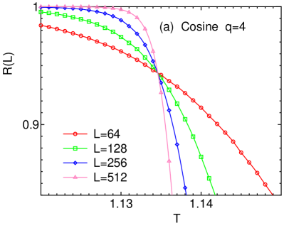
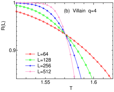
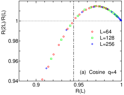
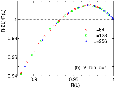
In the case of =4, the clock model becomes equivalent to two sets of Ising model, and exhibits 2nd-order transition. We show the data of =4 for both regular and Villain models for convenience. The correlation ratios of regular and Villain models for are given in Fig. 10. We observe the crossing of the data at the 2nd-order transition points. For the regular model, is exactly given by , and for the Villain model, is given by . The estimates of from the crossing of the data reproduce the exact values well. The expression of the critical value for the regular model can be given in terms of the Jacobi functions [44], and the exact numerical value becomes [30]. It is to be noted that the estimated critical value for the Villain model, 0.933, is different from the value of the regular model.
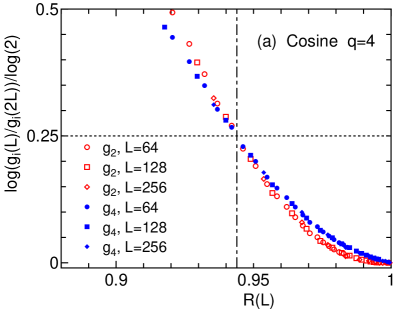
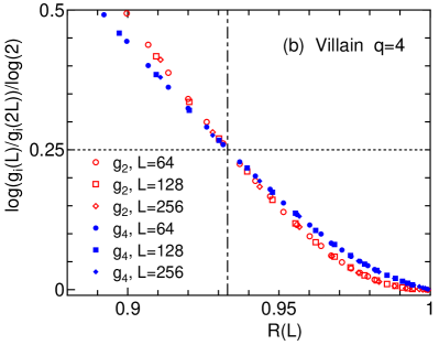
The plot of vs. for =64, 128, and 256 is given in Fig. 11. We observe a very good FSS. The value of becomes 1 at a single point, , which indicates the 2nd-order transition. It differs from the situation of the BKT transition, where the flat region in this plot, the BKT phase, exists. Since the critical value is different for the regular and the Villain models, we can say that the FSS function for vs. is not universal.
We plot with = 2, 4 in Fig. 12. We use the (red) open marks for and the (blue) closed marks for . We find that the estimate of from the value at is consistent with the exact value 1/4 for both regular and Villain models. We also note that the data with =2 and those with =4 cross at the critical value . It means that we can estimate from this plot even if we do not know or .
| regular model | Villain model | |||
|---|---|---|---|---|
| 4 | 1.1346 | 1.1346 | 1.5708 | 1.5708 |
| 5 | a) | a) | a) | a) |
| 6 | a) | a) | a) | a) |
| 6 | 0.7014(11)b) | 0.9008(6)b) | 0.8266(18)c) | 1.3269(12)c) |
| 8 | 0.4259(4)b) | 0.8936(7)b) | 0.4659(6)c) | 1.3266(11)c) |
| 12 | 0.1978(5)b) | 0.8937(6)b) | 0.2072(3)c) | 1.3272(11)c) |
| — | 0.8933(6)b) | — | 1.3306d) | |
Appendix C Phase diagram
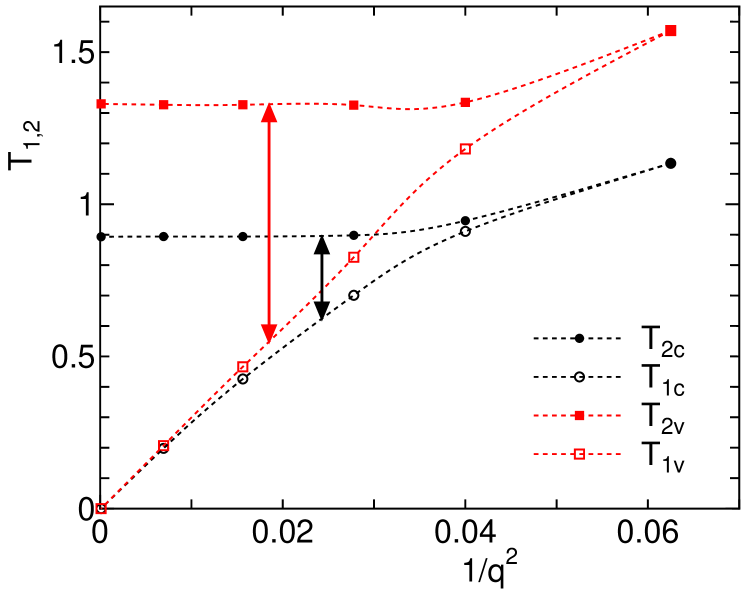
We tabulate the critical temperatures of regular and Villain types of clock model in Table 2. In this table we add some estimates of previous references [23, 42, 43]. We plot the -dependence of and of clock models in Fig. 13. There, the exact results for are also given; for the regular model the Ising singularity occurs at , and for the Villain model that occurs at . The transition temperature becomes smoothly lower with larger ; in the lowest order we find that , which is consistent with the theoretical prediction [11]. Figure 13 is the phase diagram of the clock models. The arrow indicates the BKT phase. We see a narrow BKT phase for the regular model of .
References
- [1] L. Onsager, Phys. Rev. 65, 117 (1944).
- [2] N. D. Mermin and H. Wagner, Phys. Rev. Lett. 17, 1133 (1966); P.C. Hohenberg, Phys. Rev. 158, 383 (1967).
- [3] V. L. Berezinskii, Sov. Phys. JEPT 32, 493 (1970); V. L. Berezinskii, Sov. Phys. JEPT 34, 610 (1972).
- [4] J. M. Kosterlitz and D. Thouless, J. Phys. C: Solid State Phys. 6, 1181 (1973).
- [5] J. M. Kosterlitz, J. Phys. C: Solid State Phys. 7, 1046 (1974).
- [6] D. J. Resnick et al., yd, S. Shoemaker, Phys. Rev. Lett. 47, 1542 (1981).
- [7] V. I. Marconi and D. Dominguez, Phys. Rev. Lett. 87, 017004 (2001).
- [8] Richard L. C. Vink Phys. Rev. E 90, 062132 (2014).
- [9] Y. Nahas, S. Prokhorenko, I. Kornev, and L. Bellaiche Phys. Rev. Lett. 119, 117601 (2017).
- [10] S. Elitzur, R. B. Pearson, and J. Shigemitsu, Phys. Rev. D 19, 3698 (1979).
- [11] J. V. José, L. P. Kadanoff, S. Kirkpatrick, and D. R. Nelson, Phys. Rev. B 16, 1217 (1977).
- [12] J. Tobochnik, Phys. Rev. B 26, 6201 (1982).
- [13] M. S. S. Challa and D. P. Landau, Phys. Rev. B 33, 437 (1986).
- [14] A. Yamagata and I. Ono, J. Phys. A: Math. Gen. 24, 256 (1991).
- [15] C. M. Lapilli, Phys. Rev. Lett. 96, 140603 (2006).
- [16] C.-O. Hwang, Phys. Rev. E 80, 042103 (2009).
- [17] S. K. Baek, P. Minnhagen, and B. J. Kim, Phys. Rev. E 81, 063101 (2010).
- [18] S. K. Baek and P. Minnhagen, Phys. Rev. E 82, 031102 (2010).
- [19] S. K. Baek, H. Mäkelä, P. Minnhagen and B. J. Kim, Phys. Rev. E 88, 012125 (2013).
- [20] Y. Kumano, K. Hukushima, Y. Tomita and M. Oshikawa, Phys. Rev. B 88, 104427 (2013).
- [21] C. Chatelain, J. Stat. Mech. P11022 (2014).
- [22] J. Villain, J. Phys. (Paris) 36, 581 (1975).
- [23] Y. Tomita and Y. Okabe, Phys. Rev. B 65, 184405 (2002).
- [24] R. H. Swendsen and J. S. Wang, Phys. Rev. Lett. 58, 86 (1987).
- [25] U. Wolff, Phys. Rev. Lett. 62, 361 (1989).
- [26] P. W. Kasteleyn and C. M. Fortuin, J. Phys. Soc. Jpn. Suppl. 26, 11 (1969); C. M. Fortuin and P. W. Kasteleyn, Physica (Amsterdam) 57, 536 (1972).
- [27] Y. Komura and Y. Okabe, Comp. Phys. Comm. 183, 1155 (2012); Y. Komura and Y. Okabe, Comp. Phys. Comm. 185, 1038 (2014).
- [28] D. R. Nelson and J. M. Kosterlitz, Phys. Rev. Lett. 39, 1201 (1977).
- [29] P. Minnhagen and G. G. Warren, Phys. Rev. B 24, 2526 (1981).
- [30] Y. Tomita and Y. Okabe, Phys. Rev. B 66, 180401(R) (2002).
- [31] T. Surungan, Y. Okabe, and Y. Tomita, J. Phys. A: Math. Gen. 37, 4219 (2004); T. Surungan and Y. Okabe, Phys. Rev. B 71, 188428 (2005).
- [32] K. Harada, N. Kawashima, and M. Troyer, Phys. Rev. Lett. 90, 117203 (2003).
- [33] N. Kawashima and Y. Tanabe, Phys. Rev. Lett. 98, 057202 (2007).
- [34] K. Binder, Z. Phys. B 43, 119 (1981).
- [35] H. G. Katzgraber, M. Körner, and A. P. Young, Phys. Rev. B 73, 224432 (2006).
- [36] Y. Komura and Y. Okabe, J. Phys. A: Math. Gen. 44, 015002 (2011).
- [37] S. Caraccido, R. G. Edwards, S. J. Ferreira, A. Pelissetto, and A. D. Sokal, Phys. Rev. Lett. 74, 2969 (1995).
- [38] J. Salas and A. D. Sokal, J. Stat. Phys. 88, 567 (1997).
- [39] W. Janke, Phys. Rev. B 55, 3580 (1997).
- [40] H. Weber and P. Minnhagen, Phys. Rev. B 37, 5986 (1988).
- [41] K. Harada and N. Kawashima, Phys. Rev. B 55, 011949(R) (1997).
- [42] T. Takayama, Master Thesis, Tokyo Metropolitan University (2007).
- [43] M. Hasenbusch and K. Pinn, J. Phys. A 30, 63 (1997); M. Hasenbusch, J. Stat. Mech. P12006 (2008).
- [44] P. Di Francesco, H. Saleur, and J.-B. Suber, Nucl. Phys. B 290 [FS20], 527 (1987); Europhys. Lett. 5, 95 (1988).
- [45] M. Hasenbusch: J. Phys. A: Math. Gen. 38, 5869 (2005).
- [46] Kinetik Orderin paper, 2017 J. Phys. A: Math. Gen. 38, 5869 (2005).