Semi-Supervised Regression using Cluster Ensemble and Low-Rank Co-Association Matrix Decomposition under Uncertainties

Abstract

In this paper, we solve a semi-supervised regression problem. Due to the lack of knowledge about the data structure and the presence of random noise, the considered data model is uncertain. We propose a method which combines graph Laplacian regularization and cluster ensemble methodologies. The co-association matrix of the ensemble is calculated on both labeled and unlabeled data; this matrix is used as a similarity matrix in the regularization framework to derive the predicted outputs. We use the low-rank decomposition of the co-association matrix to significantly speedup calculations and reduce memory. Numerical experiments using the Monte Carlo approach demonstrate robustness, efficiency, and scalability of the proposed method.

1 Introduction

Machine learning problems can be classified as supervised, unsupervised and semi-supervised. Let data set $\mathbf{X}=\{x_{1},\dots,x_{n}\}$ be given, where $x_{i}\in\mathbb{R}^{d}$ is feature vector, $d$ is feature space dimensionality. In a supervised learning context, we are given an additional set $Y=\{y_{1},\dots,y_{n}\}$ of target feature values (labels) for all data points, $y_{i}\in D_{Y}$, where $D_{Y}$ is target feature domain. In the case of supervised classification, the domain is an unordered set of categorical values (classes, patterns). In case of supervised regression, the domain $D_{Y}\subseteq\mathbb{R}$. Using this information (which can be thought as provided by a certain “teacher”), it is necessary to find a decision function $y=f(x)$ (classifier, regression model) for predicting target feature values for any new data point $x\in\mathbb{R}^{d}$ from the same statistical population. The function should be optimal in some sense, e.g., give minimal value to the expected losses.

In an unsupervised learning setting, the target feature values are not provided. The problem of cluster analysis, which is an important direction in unsupervised learning, consists in finding a partition $P=\{C_{1},\dots,C_{K}\}$ of $\mathbf{X}$ on a relatively small number of homogeneous clusters describing the structure of data. As a criterion of homogeneity, it is possible to use a functional dependent on the scatter of observations within groups and the distances between clusters. The desired number of clusters is either a predefined parameter or should be found in the best way.

We note that since the final cluster partition is uncertain due to random noise in sample data, lack of knowledge about the feature set and the data structure, parameters, weights, and initialization settings, a set of different cluster partitions is calculated. Then a final cluster partition is formed.

In semi-supervised learning problems, the target feature values are known only for a part of data set $X_{1}\subset\mathbf{X}$. It is possible to assume that $X_{1}=\{x_{1},\dots,x_{n_{1}}\}$, and the unlabeled part is $X_{0}=\{x_{n_{1}+1},\dots,x_{n}\}$. The set of labels for points from $X_{1}$ is denoted by $Y_{1}=\{y_{1},\dots,y_{n_{1}}\}$. It is required to predict target feature values as accurately as possible either for given unlabeled data $X_{0}$ (i.e., perform transductive learning) or for arbitrary new observations from the same statistical population (inductive learning). In dependence of the type of the target feature, one may consider semi-supervised classification or semi-supervised regression problems [29].

The task of semi-supervised learning is important because in many real-life problems only a small part of available data can be labeled due to the large cost of target feature registration. For example, manual annotation of digital images is rather time-consuming. Therefore labels can be attributed to only a small part of pixels. To improve prediction accuracy, it is necessary to use information contained in both labeled and unlabeled data. An important application is hyperspectral image semi-supervised classification [7].

In this paper, we consider a semi-supervised regression problem in the transductive learning setting. In semi-supervised regression, the following types of methods can be found in the literature [17]: co-training [28], semi-supervised kernel regression [24], graph-based and spectral regression methods [25, 11, 26], etc.

We propose a novel semi-supervised regression method using a combination of graph Laplacian regularization technique and cluster ensemble methodology. Graph regularization (sometimes called manifold regularization) is based on the assumption which states that if two data points are on the same manifold, then their corresponding labels are close to each other. A graph Laplacian is used to measure the smoothness of the predictions on the data manifold including both labeled and unlabeled data [27, 1].

Ensemble clustering aims at finding consensus partition of data using some base clustering algorithms. As a rule, application of this methodology allows one to get a robust and effective solution, especially in case of uncertainty in the data model. Properly organized ensemble (even composed of ”weak” learners) significantly improves the overall clustering quality [6].

Different schemes for applying ensemble clustering for semi-supervised classification were proposed in [23, 2]. The suggested methods are based on the hypothesis which states that a preliminary ensemble allows one to restore more accurately metric relations in data in noise conditions. The obtained co-association matrix (CM) depends on the outputs of clustering algorithms and is less noise-addicted than a conventional similarity matrix. This increases the prediction quality of the methods.

The same idea is pivotal in the proposed semi-supervised regression method. We assume a statistical connection between the clustering structure of data and the predicted target feature. Such a connection may exist, for example, when some hidden classes are present in data, and the belonging of objects to the same class influences the proximity of their responses.

To decrease the computational cost and the storage requirement and to increase the scalability of the method, we suggest usage of low-rank (or hierarchical) decomposition of CM. This decomposition will reduce the numerical cost and storage from cubic to (log-)linear [15].

Parametric approximations, given by generalized linear models, as well as nonlinear models, given by neural networks were compared in [5].

In the rest of the paper, we describe the details of the suggested method. Numerical experiments are presented in the correspondent section. Finally, we give concluding remarks.

2 Combined semi-supervised regression and ensemble clustering

2.1 Graph Laplacian regularization

We consider a variant of graph Laplacian regularization in semi-supervise transductive regression which solves the following optimization problem:

find $f^{*}$ such that $f^{*}=\arg\min\limits_{f\in\mathbb{R}^{n}}Q(f)$, where

$$Q(f):=\frac{1}{2}\left(\sum\limits_{x_{i}\in X_{1}}(f_{i}-y_{i})^{2}+\alpha\sum\limits_{x_{i},x_{j}\in\mathbf{X}}w_{ij}(f_{i}-f_{j})^{2}+\beta||f||^{2}\right),$$ (1)

$f=(f_{1},\dots,f_{n})$ is a vector of predicted outputs: $f_{i}=f(x_{i})$; $\alpha,\beta>0$ are regularization parameters, $W=(w_{ij})$ is data similarity matrix. The degree of similarity between points $x_{i}$ and $x_{j}$ can be calculated using appropriate function, for example from the Matérn family [21]. The Matérn function depends only on the distance $h:=\|x_{i}-x_{j}\|$ and is defined as $W(h)=\frac{\sigma^{2}}{2^{\nu-1}\Gamma(\nu)}\left(\frac{h}{\ell}\right)^{\nu}K_{\nu}\left(\frac{h}{\ell}\right)$ with three parameters $\ell$, $\nu$, and $\sigma^{2}$. For instance, $\nu=1/2$ gives the well-known exponential kernel $W(h)=\sigma^{2}\exp(-h/\ell)$, and $\nu=\infty$ gives the Gaussian kernel $W(h)=\sigma^{2}\exp(-h^{2}/2\ell^{2})$.

In this paper we also use RBF kernel with parameter $\ell$: $w_{ij}=\exp(-\frac{\|x_{i}-x_{j}\|^{2}}{2\ell^{2}})$.

The first term in right part of (1) minimizes fitting error on labeled data; the second term aims to obtain ”smooth” predictions on both labeled and unlabeled sample; the third one is Tikhonov’s regularizer.

Let graph Laplacian be denoted by $L=D-W$ where $D$ be a diagonal matrix defined by $D_{ii}=\sum\limits_{j}w_{ij}$. It is easy to show (see, e.g., [1, 27]) that

$$\sum\limits_{x_{i},x_{j}\in\mathbf{X}}w_{ij}(f_{i}-f_{j})^{2}=2f^{T}Lf.$$ (2)

Let us introduce vector $Y_{1,0}=(y_{1},\dots,y_{n_{1}},\underbrace{0,\dots,0}_{n-n_{1}})^{T}$, and let $G$ be a diagonal matrix:

$$G=diag(G_{11}\dots,G_{nn}),\;G_{ii}=\left\{{}^{\beta+1,\;i=1,\dots,n_{1}}_{\beta,\;i=n_{1}+1,\dots,n,}\right..$$ (3)

Differentiating $Q(f)$ with respect to $f$, we get

$$\frac{\partial Q}{\partial f}\mid_{f=f^{*}}=Gf^{*}+\alpha Lf^{*}-Y_{1,0}=0,$$

hence

$$f^{*}=(G+\alpha L)^{-1}\;Y_{1,0}$$ (4)

under the condition that the inverse of matrix sum exists (note that the regularization parameters $\alpha,\beta$ can be selected to guaranty the well-posedness of the problem). Numerical methods such as Tikhonov or Lavrentiev regularization [22] can also be used to obtain the predictions.

2.2 Co-association matrix of cluster ensemble

In the proposed method, we use a co-association matrix of cluster ensemble as similarity matrix in (1). Co-association matrix is calculated as a preliminary step in the process of cluster ensemble design with various clustering algorithms or under variation across a given algorithm’s parameter settings [12].

Let us consider a set of partition variants $\{P_{l}\}_{l=1}^{r}$, where $P_{l}=\{C_{l,1},\dots,C_{l,K_{l}}\}$, $C_{l,k}\subset\mathbf{X}$, $C_{l,k}\bigcap C_{l,k^{\prime}}=\varnothing$, $K_{l}$ is number of clusters in $l$th partition. For each $P_{l}$ we determine matrix $H_{l}=(h_{l}(i,j))_{i,j=1}^{n}$ with elements indicating whether a pair $x_{i}$, $x_{j}$ belong to the same cluster in $l$th variant or not: $h_{l}(i,j)=\mathbb{I}[c_{l}(x_{i})=c_{l}(x_{j})]$, where $\mathbb{I}(\cdot)$ is indicator function ($\mathbb{I}[true]=1$, $\mathbb{I}[false]=0$), $c_{l}(x)$ is cluster label assigned to $x$. The weighted averaged co-association matrix (WACM) is defined as follows:

$$H=(H(i,j))_{i,j=1}^{n},\quad H(i,j)=\sum\limits_{l=1}^{r}w_{l}H_{l}(i,j)$$ (5)

where $w_{1},\dots,w_{r}$ are weights of ensemble elements, $w_{l}\geq 0$, $\sum w_{l}=1$. The weights should reflect the “importance” of base clustering variants in the ensemble [4] and be dependent on some evaluation function $\Gamma$ (cluster validity index, diversity measure) [3]: $w_{l}=\gamma_{l}/\sum\limits_{l^{\prime}}\gamma_{l^{\prime}}$, where $\gamma_{l}=\Gamma(l)$ is an estimate of clustering quality for the $l$th partition (we assume that a larger value of $\Gamma$ manifests better quality).

In the methodology presented in this paper, the elements of WACM are viewed as similarity measures learned by the ensemble. In a sense, the matrix specifies the similarity between objects in a new feature space obtained utilizing some implicit transformation of the initial data. The following property of WACM allows increasing the processing speed.

Proposition 1. Weighted averaged co-association matrix admits low-rank decomposition in the form:

$$H=BB^{T},\;B=[B_{1}B_{2}\dots B_{r}]$$ (6)

where $B$ is a block matrix, $B_{l}=\sqrt{w_{l}}\,A_{l}$, $A_{l}$ is ($n\times K_{l}$) cluster assignment matrix for $l$th partition: $A_{l}(i,k)=\mathbb{I}[c(x_{i})=k]$, $i=1,\dots,n$, $k=1,\dots,K_{l}$.

The proof is fairly straightforward and is omitted here for the sake of brevity. As a rule, $m=\sum_{l}K_{l}\ll n$, thus (6) gives us an opportunity of saving memory by storing $(n\times m)$ sparse matrix instead of full $(n\times n)$ co-association matrix. The complexity of matrix-vector multiplication $H\cdot x$ is decreased from $O(n^{2})$ to $O(nm)$.

2.3 Cluster ensemble and graph Laplacian regularization

Let us consider graph Laplacian in the form: $L^{\prime}=D^{\prime}-H$, where $D^{\prime}=\text{diag}(D^{\prime}_{11},$ $\dots,D^{\prime}_{nn})$, $D^{\prime}_{ii}=\sum\limits_{j}H(i,j)$. We have:

$$\small D^{\prime}_{ii}=\sum\limits_{j=1}^{n}\sum\limits_{l=1}^{r}w_{l}\sum\limits_{k=1}^{K_{l}}A_{l}(i,k)A_{l}(j,k)=\\ \sum\limits_{l=1}^{r}w_{l}\sum\limits_{k=1}^{K_{l}}A_{l}(i,k)\sum\limits_{j=1}^{n}A_{l}(j,k)=\sum\limits_{l=1}^{r}w_{l}N_{l}(i)$$ (7)

where $N_{l}(i)$ is the size of the cluster which includes point $x_{i}$ in $l$th partition variant.

Substituting $L^{\prime}$ in (4), we obtain cluster ensemble based predictions of output feature in semi-supervised regression:

$$f^{**}=(G+\alpha L^{\prime})^{-1}\;Y_{1,0}.$$ (8)

Using a low-rank representation of $H$, this expression can be transformed into the form which involves more efficient matrix operations:

$$f^{**}=(G+\alpha D^{\prime}-\alpha BB^{T})^{-1}\;Y_{1,0}.$$

In linear algebra, the following Woodbury matrix identity is known:

$$(S+UV)^{-1}=S^{-1}-S^{-1}U(I+VS^{-1}U)^{-1}VS^{-1},$$

where $S\in\mathbb{R}^{n\times n}$ is invertible matrix, $U\in\mathbb{R}^{n\times m}$ and $V\in\mathbb{R}^{m\times n}$. We can denote $S=G+\alpha D^{\prime}$ and get

$$S^{-1}=\text{diag}(1/(G_{11}+\alpha D^{\prime}_{11}),\dots,1/(G_{nn}+\alpha D^{\prime}_{nn})),$$ (9)

where $G_{ii},D^{\prime}_{ii}$, $i=1,\dots,n$ are defined in (3) and (7) correspondingly.

Now it is clear that the following statement is valid:

Proposition 2. Cluster ensemble based target feature prediction vector (8) can be calculated using low-rank decomposition as follows:

$$f^{**}=(S^{-1}+\alpha S^{-1}B(I-\alpha B^{T}S^{-1}B)^{-1}BS^{-1})\;Y_{1,0}$$ (10)

where matrix $B$ is defined in (6) and $S^{-1}$ in (9).

Note that in (10) we need to invert significantly smaller ($m\times m$) sized matrix instead of ($n\times n$) in (8). The overall computational complexity of (10) can be estimated as $O(nm+m^{3})$.

The outline of the suggested algorithm of semi-supervised regression based on the low-rank decomposition of the co-association matrix (SSR-LRCM) is as follows.

Algorithm SSR-LRCM

Input:

${{\mathbf{X}}}$: dataset including both labeled and unlabeled sample;

$Y_{1}$: target feature values for labeled instances;

$r$: number of runs for base clustering algorithm $\mu$;

$\mathbf{\Omega}$: set of parameters (working conditions) of clustering algorithm.

Output:

$f^{**}$: predictions of target feature for labeled and unlabeled objects.

Steps:

1. Generate $r$ variants of clustering partition with algorithm $\mu$ for working parameters randomly chosen from $\mathbf{\Omega}$; calculate weights $w_{1},\dots,w_{r}$ of variants.

2. Find graph Laplacian in low-rank representation using matrices $B$ in (6) and $D^{\prime}$ in (7);

3. Calculate predictions of target feature according to (10).

end.

In the implementation of SSR-LRCM, we use K-means as base clustering algorithm which has linear complexity with respect to data dimensions.

3 Hierarchical Approximation

In this section we discuss the case if matrices $W$ and $H$ do not have any low-rank decomposition or this low-rank is expensive (e.g., the rank is comparable with $n$). In that case then one can try to apply, so-called, hierarchical matrices ($\mathcal{H}$-matrices), introduced in [14], [15].

The $\mathcal{H}$-matrix format has a log-linear computational cost and storage. The $\mathcal{H}$-matrix technique allows us to efficiently work with general matrices $W$ and $H$ (and not only with structured ones like Toeplitz, circulant or three diagonal). Another advantage is that all linear algebra operations from Sections 2.1 and 2.2 preserve (or only slightly increase) the rank $k$ inside of each sub-block.

There are many implementations of $\mathcal{H}$-matrices exist, e.g., the HLIB library (http://www.hlib.org/), $\mathcal{H}^{2}$-library (https://github.com/H2Lib), and HLIBpro library (https://www.hlibpro.com/). We used the HLIBpro library, which is actively supported commercial, robust, parallel, very tuned, and well tested library. Applications of the $\mathcal{H}$-matrix technique to the graph Laplacian can be found in the HLIBpro library, and to covariance matrices in [16] and in [19].

The $\mathcal{H}$-matrix technique is defined as a hierarchical partitioning of a given matrix into sub-blocks followed by the further approximation of the majority of these sub-blocks by low-rank matrices. Figure 1 shows an example of the $\mathcal{H}$-matrix approximation $\widetilde{W}$ of an $n\times n$ matrix $W$, $n=16000$ and its Cholesky factor $\widetilde{U}$, where $\widetilde{W}=\widetilde{U}\widetilde{U}^{\top}$. The dark (or red) blocks indicate the dense matrices and the grey (green) blocks indicate the rank-$k$ matrices; the number inside each block is its rank. The steps inside the blocks show the decay of the singular values in $\log$ scale. The Cholesky factorization is needed for computing the inverse, $\widetilde{W}^{-1}=(\widetilde{U}\widetilde{U}^{\top})^{-1}=\widetilde{U}^{-\top}\widetilde{U}^{-1}$. This way is cheaper as computing the inverse directly.

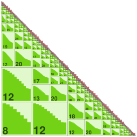
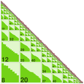
Figure 1: (left) An example of the $\mathcal{H}$-matrix approximation $\widetilde{W}$ of an $n\times n$ matrix $W$, $n=16000$. (right) The corresponding Cholesky factor $\widetilde{U}$, where $\widetilde{W}=\widetilde{U}\widetilde{U}^{\top}$.

To define which sub-blocks can be approximated well by low-rank matrices and which cannot, a so-called admissibility condition is used (see more details in [19]). There are different admissibility conditions possible: weak, strong, domain decomposition based. Each one results in a new subblock partitioning. Blocks that satisfy the admissibility condition can be approximated by low-rank matrices; see [14].

On the first step, the matrix is divided into four sub-blocks. Then each (or some) sub-block(s) is (are) divided again and again hierarchically until sub-blocks are sufficiently small. The procedure stops when either one of the sub-block sizes is $n_{\mbox{min}}$ or smaller (typically $n_{\mbox{min}}\leq 128$), or when this sub-block can be approximated by a low-rank matrix.

Another important question is how to compute these low-rank approximations. One (heuristic) possibility is the Adaptive Cross Approximation (ACA) algorithm [15], which performs the approximations with a linear complexity $\mathcal{O}(kn)$ in contrast to $\mathcal{O}(n^{3})$ by the standard singular value decomposition (SVD).

The storage requirement of $\widetilde{W}$ and the matrix vector multiplication cost $\mathcal{O}(kn\log n)$, the matrix-matrix addition costs $\mathcal{O}(k^{2}n\log n)$, and the matrix-matrix product and the matrix inverse cost $\mathcal{O}(k^{2}n\log^{2}n)$; see [14]. In Table 1 we show dependence of the two matrix errors on the $\mathcal{H}$-matrix rank $k$ for the Matérn function with parameters $\ell=\{0.25,0.75\}$, $\nu=1.5$, and $x_{i},x_{j}\in[0,1]^{2}$. We can bound the relative error $\|W^{-1}-\widetilde{W}^{-1}\|/\|W^{-1}\|$ for the approximation of the inverse as

$$\frac{\|W^{-1}-\widetilde{W}^{-1}\|}{\|W^{-1}\|}=\frac{\|({I}-\widetilde{W}^{-1}W)W^{-1}\|}{\|W^{-1}\|}\leq\|({I}-\widetilde{W}^{-1}W)\|.$$

$\|({I}-\widetilde{W}^{-1}W)\|_{2}$ can be estimated by few steps of the power iteration method. The rank $k\leq 20$ is not sufficient to approximate the inverse.The spectral norms of $\tilde{W}$ are $\|\widetilde{W}_{(\ell=0.25)}\|_{2}=720$ and $\|\widetilde{W}_{(\ell=0.75)}\|_{2}=1068$.

Table 1: Convergence of the $\mathcal{H}$-matrix approximation error vs. the $\mathcal{H}$-matrix rank $k$ of a Matérn function with parameters $\ell=\{0.25,0.75\}$, $\nu=1.5$, $x_{i},x_{j}\in[0,1]^{2}$, $n=16{,}641$, see more in [18]

$k$	$\|W-\widetilde{W}\|_{2}$		$\|{I}-\widetilde{W}^{-1}{W}\|_{2}$
	$\ell=0.25$	$\ell=0.75$	$\ell=0.25$	$\ell=0.75$
20	5.3e-7	2e-7	4.5	72
30	1.3e-9	5e-10	4.8e-3	20
40	1.5e-11	8e-12	7.4e-6	0.5
50	2.0e-13	1.5e-13	1.5e-7	0.1

Table 2 shows the computational time and storage for the $\mathcal{H}$-matrix approximations [18, 19]. These computations are done with the parallel $\mathcal{H}$-matrix toolbox, HLIBpro. The number of computing cores is 40, the RAM memory 128GB. It is important to note that the computing time (columns 2 and 5) and the storage cost (columns 3 and 6) are growing nearly linearly with $n$. Additionally, we provide the accuracy of the $\mathcal{H}$-Cholesky inverse.

Table 2: Computing times and storage costs of $\widetilde{W}\in\mathbb{R}^{n\times n}$. Accuracy in each sub-block is $\varepsilon=10^{-7}$.

$n$	$\widetilde{W}$			$\widetilde{{U}}\widetilde{{U}}^{\top}$
	time	size	kB/$n$	time	size	$\|{I}-(\widetilde{{U}}\widetilde{{U}}^{\top})^{-1}{W}\|_{2}$
	sec	MB		sec	MB
128,000	7.7	1160	9.5	36.7	1310	$3.8\cdot 10^{-5}$
256,000	13	2550	10.5	64.0	2960	$7.1\cdot 10^{-5}$
512,000	23	4740	9.7	128	5800	$7.1\cdot 10^{-4}$
1,000,000	53	11260	11	361	13910	$3.0\cdot 10^{-4}$
2,000,000	124	23650	12.4	1001	29610	$5.2\cdot 10^{-4}$

3.1 $\mathcal{H}$-matrix approximation of regularized graph Laplacian

We rewrite formulas from Sections 2.1 - 2.3 in the $\mathcal{H}$-matrix format. Let $\tilde{W}$ be an $\mathcal{H}$-matrix approximation of $W$. The new optimization problem will be:

find $\tilde{f}^{*}$ such that $\tilde{f}^{*}=\arg\min\limits_{f\in\mathbb{R}^{n}}\tilde{Q}(f)$, where

$$\tilde{Q}(f):=\frac{1}{2}\left(\sum\limits_{x_{i}\in X_{1}}(f_{i}-y_{i})^{2}+\alpha\sum\limits_{x_{i},x_{j}\in\mathbf{X}}\tilde{w}_{ij}(f_{i}-f_{j})^{2}+\beta\|f\|^{2}\right).$$ (11)

Using (2) and assuming that the $\mathcal{H}$-matrix approximation error $\|\tilde{L}-L\|\leq\varepsilon$, obtain

$$\|\tilde{Q}(f)-Q(f)\|\leq\alpha\left(f^{\top}\tilde{L}f-f^{\top}{L}f\right)\leq\alpha\|f\|^{2}\|\tilde{L}-L\|=\|f\|^{2}\varepsilon.$$ (12)

Let the approximate graph Laplacian be denoted by $\tilde{L}=\tilde{D}-\tilde{W}$ where $\tilde{D}$ be a diagonal matrix defined by $\tilde{{D}}_{ii}=\sum\limits_{j}\tilde{w}_{ij}$. Differentiating $\tilde{Q}(f)$ with respect to $f$, we get

$$\frac{\partial\tilde{Q}}{\partial f}\mid_{f=\tilde{f}^{*}}={G}\tilde{f}^{*}+\alpha\tilde{L}\tilde{f}^{*}-Y_{1,0}=0,$$

hence

$$\tilde{f}^{*}=({G}+\alpha\tilde{L})^{-1}\;Y_{1,0}$$ (13)

The impact of the $\mathcal{H}$-matrix approximation error could be measured as follows

$$\|\tilde{f}^{*}-f^{*}\|\leq\|({G}+\alpha\tilde{L})^{-1}-({G}+\alpha{L})^{-1}\|\cdot\|Y_{1,0}\|$$ (14)

or

$$\|\tilde{f}^{*}-f^{*}\|\leq\|(I+\alpha G^{-1}\tilde{L})^{-1}-({I}+\alpha G^{-1}{L})^{-1}\|\|G\|\cdot\|Y_{1,0}\|$$ (15)

Now, if matrix norm (e.g., spectral norm) of $\alpha G^{-1}\tilde{L}$ is smaller than 1, we can write

$$(I+\alpha G^{-1}\tilde{L})^{-1}=I-\alpha G^{-1}\tilde{L}+\alpha^{2}G^{-2}\tilde{L}^{2}-\alpha^{3}G^{-3}\tilde{L}^{3}+\ldots$$ (16)

and

$$\|(I+\alpha G^{-1}\tilde{L})^{-1}-(I+\alpha G^{-1}{L})^{-1}\|$$

$$\leq\alpha\|G^{-1}(\tilde{L}-L)\|+\alpha\|G^{-2}(\tilde{L}^{2}-L^{2})\|+\alpha^{2}\|G^{-3}(\tilde{L}^{3}-L^{3})\|+\ldots$$

In general, the assumption $\|W-\tilde{W}\|\leq\varepsilon$ is not sufficient to say something about the error $\|({W}^{-1}-\tilde{W}^{-1}\|$ because the later is proportional to the condition number of $\tilde{W}$, which could be very large. The reason for a large condition number is that the smallest eigenvalue could lie very close to zero. In this case some regularization may help (e.g., adding a positive number to all diagonal elements, similar to Tikhonov regularization). In this sense, the diagonal matrix $G$ helps to bound the error $\|({G}+\alpha\tilde{L})^{-1}-({G}+\alpha{L})^{-1}\|$. We remind that by one of the properties of the graph Laplacian states $\det(L)=0$ and $L$ is not invertible. Assume now that instead of Eq. 5 we have an $\mathcal{H}$-matrix approximation $\tilde{H}$ of $H$. Then the $\mathcal{H}$-matrix approximation of the graph Laplacian will be $\tilde{L}^{\prime}=\tilde{D}^{\prime}-\tilde{H}$, where $\tilde{D}^{\prime}=\text{diag}(\tilde{D}^{\prime}_{11},$ $\dots,\tilde{D}^{\prime}_{nn})$, $\tilde{D}^{\prime}_{ii}=\sum\limits_{j}\tilde{H}(i,j)$. It is important to notice that the computational cost of computing $\tilde{D}$ is $\mathcal{O}(kn\log n)$, $k\ll n$.

Substituting $\tilde{L}^{\prime}$ in (13), we obtain cluster ensemble based predictions of output feature in semi-supervised regression:

$$\tilde{f}^{**}=({G}+\alpha\tilde{L}^{\prime})^{-1}\;Y_{1,0}.$$ (17)

Here we cannot apply the Woodbury formula, but we also do not need it since the computational cost of computing $({G}+\alpha\tilde{L}^{\prime})^{-1}$ in the $\mathcal{H}$-matrix format is just $\mathcal{O}(k^{2}n\log^{2}n)$.

The SSR-LRCM Algorithm requires only minor changes, namely, in the second step we compute an $\mathcal{H}$-matrix representation of the graph Laplacian and on the third step calculate predictions of target feature according to (17). The total computational complexity is log-linear.

4 Numerical experiments

In this section we describe numerical experiments with the proposed SSR-LRCM algorithm. The aim of experiments is to confirm the usefulness of involving cluster ensemble for similarity matrix estimation in semi-supervised regression. We experimentally evaluate the regression quality on a synthetic and a real-life example.

4.1 First example with two clusters and artificial noisy data

In the first example we consider datasets generated from a mixture of two multidimensional normal distributions $\mathcal{N}(a_{1},\sigma_{X}I)$, $\mathcal{N}(a_{2},\sigma_{X}I)$ under equal weights; $a_{1}$, $a_{2}$ $\in\mathbb{R}^{d}$, $d=8$, $\sigma_{X}$ is a parameter. Usually such type of data is applied for a classifier evaluation; however it is possible to introduce a real valued attribute $Y$ as a predicted feature and use it in regression analysis. Let $Y$ equal $1+\varepsilon$ for points generated from the first distribution component, otherwise $Y=2+\varepsilon$, where $\varepsilon$ is a Gaussian random value with zero mean and variance $\sigma^{2}_{\varepsilon}$. To study the robustness of the algorithm, we also generate two independent random variables following uniform distribution $\mathcal{U}(0,\sigma_{X})$ and use them as additional “noisy” features.

In Monte Carlo modeling, we repeatedly generate samples of size $n$ according to the given distribution mixture. In the experiment, 10% of the points selected at random from each component compose the labeled sample; the remaining ones are included in the unlabeled part. To study the behavior of the algorithm in the presence of noise, we also vary parameter $\sigma_{\varepsilon}$ for the target feature.

In SSR-LRCM, we use $K$-means as a base clustering algorithm. The ensemble variants are designed by random initialization of centroids (number of clusters equals two). The ensemble size is $r=10$. The wights of ensemble elements are the same: $w_{l}\equiv 1/r$. The regularization parameters $\alpha,\beta$ have been estimated using grid search and cross-validation technique. In our experiments, the best results have been obtained for $\alpha=1$, $\beta=0.001$, and $\sigma_{X}=5$.

For the comparison purposes, we consider the method (denoted as SSR-RBF) which uses the standard similarity matrix evaluated with RBF kernel. Different values of parameter $\ell$ were considered and the quasi-optimal $\ell=4.47$ was taken. The output predictions are calculated according to formula (4).

The quality of prediction is estimated as Root Mean Squared Error: $\text{RMSE}=\sqrt{\frac{1}{n}\sum(y_{i}^{\text{true}}-f_{i})^{2}}$, where $y_{i}^{\text{true}}$ is a true value of response feature specified by the correspondent component. To make the results more statistically sound, we have averaged error estimates over 40 Monte Carlo repetitions and compare the results by paired two sample Student’s t-test.

Table 3 presents the results of experiments. In addition to averaged errors, the table shows averaged execution times for the algorithms (working on dual-core Intel Core i5 processor with a clock frequency of 2.8 GHz and 4 GB RAM). For SSR-LRCM, we separately indicate ensemble generation time $t_{\text{ens}}$ and low-rank matrix operation time $t_{\text{matr}}$ (in seconds). The obtained $p$-values for Student’s $t$-test are also taken into account. A $p$-value less than the given significance level (e.g., $0.05$) indicates a statistically significant difference between the performance estimates.

Table 3: Results of experiments with a mixture of two distributions. Significantly different RMSE values ($p$-value $<10^{-5}$) are in bold. For $n=10^{5}$ and $n=10^{6}$, SSR-RBF failed due to unacceptable memory demands.

$n$	$\;\;\sigma_{\varepsilon}$	SSR-LRCM			SSR-RBF
		RMSE	$\;t_{\text{ens }}$ (sec)	$t_{\text{matr }}$ (sec)	RMSE	time (sec)
1000	0.01	0.052	0.06	0.02	0.085	0.10
	0.1	0.054	0.04	0.04	0.085	0.07
	0.25	0.060	0.04	0.04	0.102	0.07
3000	0.01	0.049	0.06	0.02	0.145	0.74
	0.1	0.051	0.06	0.02	0.143	0.75
	0.25	0.053	0.07	0.02	0.150	0.79
7000	0.01	0.050	0.16	0.08	0.228	5.70
	0.1	0.050	0.16	0.08	0.229	5.63
	0.25	0.051	0.14	0.07	0.227	5.66
$10^{5}$	0.01	0.051	1.51	0.50	-	-
$10^{6}$	0.01	0.051	17.7	6.68	-	-

The results show that the proposed SSR-LRCM algorithm has significantly smaller prediction error than SSR-RBF. At the same time, SSR-LRCM has run much faster, especially for medium sample size. For a large volume of data ($n=10^{5}$, $n=10^{6}$) only SSR-LRCM has been able to find a solution, whereas SSR-RBF has refused to work due to unacceptable memory demands (74.5GB and 7450.6GB correspondingly).

4.2 Second example with 10-dimensional real Forest Fires dataset

In the second example, we consider Forest Fires dataset [9]. It is necessary to predict the burned area of forest fires, in the northeast region of Portugal, by using meteorological and other information. Fire Weather Index (FWI) System is applied to get feature values. FWI System is based on consecutive daily observations of temperature, relative humidity, wind speed, and 24-hour rainfall. We use the following numerical features:

• X-axis spatial coordinate within the Montesinho park map;

• Y-axis spatial coordinate within the Montesinho park map;

• Fine Fuel Moisture Code;

• Duff Moisture Code;

• Initial Spread Index;

• Drought Code;

• temperature in Celsius degrees;

• relative humidity;

• wind speed in km/h;

• outside rain in mm/m2;

• the burned area of the forest in ha (predicted feature).

This problem is known as a difficult regression task [10], in which the best RMSE was attained by the naive mean predictor. We use quantile regression approach: the transformed quartile value of response feature should be predicted.

The following experiment’s settings are used. The volume of labeled sample is 10% of overall data; the cluster ensemble architecture is the same as in the previous example. $K$-means base algorithm with 10 clusters with ensemble size $r=10$ is used. Other parameters are $\alpha=1$, $\beta=0.001$, the SSR-RBF parameter is $\ell=0.1$. The number of generations of the labeled samples is 40.

As a result of modeling, the averaged error rate for SSR-LRCM has been evaluated as RMSE$=1.65$. For SSR-RBF, the averaged RMSE is equal to $1.68$. The $p$-value which equals $0.001$ can be interpreted as indicating the statistically significant difference between the quality estimates.

Conclusion

In this work, we solved the regression problem to forecast the unknown value $Y$. For this we have introduced a semi-supervised regression method SSR-LRCM based on cluster ensemble and low-rank co-association matrix decomposition. We used a scheme of a single clustering algorithm which obtains base partitions with random initialization.

The proposed method combines graph Laplacian regularization and cluster ensemble methodologies. Low-rank or hierarchical decomposition of the co-association matrix gives us a possibility to speedup calculations and save memory from cubic to (log-)linear.

There are a number of arguments for the usefulness of ensemble clustering methodology. The preliminary ensemble clustering allows one to restore more accurately metric relations between objects under noise distortions and the existence of complex data structures. The obtained similarity matrix depends on the outputs of clustering algorithms and is less noise-addicted than the conventional similarity matrices (eg., based on Euclidean distance). Clustering with a sufficiently large number of clusters can be viewed as Learning Vector Quantization known for lowering the average distortion in data.

The efficiency of the suggested SSR-LRCM algorithm was confirmed experimentally. Monte Carlo experiments have demonstrated statistically significant improvement of regression quality and decreasing in running time for SSR-LRCM in comparison with analogous SSR-RBF algorithm based on standard similarity matrix.

In future works, we plan to continue studying theoretical properties and performance characteristics of the proposed method. Development of iterative methods for graph Laplacian regularization is another interesting direction, especially in large-scale machine learning problems. We will further research theoretical and numerical properties of the $\mathcal{H}$-matrix approximation of $W$ and $H$. Applications of the method in various fields are also planned, especially for spacial data processing and analysis of genetic sequences.

References

- [1] Belkin M., Niyogi P., Sindhwani V. Manifold Regularization: A Geometric Framework for Learning from Labeled and Unlabeled Examples. J. Mach. Learn. Res. Vol. 7, no. Nov. 2399-2434 (2006)
- [2] Berikov V., Karaev N., Tewari A. Semi-supervised classification with cluster ensemble. In Engineering, Computer and Information Sciences (SIBIRCON), 2017 International Multi-Conference. 245–250. IEEE. (2017)
- [3] Berikov V.B. Construction of an optimal collective decision in cluster analysis on the basis of an averaged co-association matrix and cluster validity indices. Pattern Recognition and Image Analysis. 27(2), 153–165 (2017)
- [4] Berikov V.B., Litvinenko A., The influence of prior knowledge on the expected performance of a classifier. Pattern recognition letters 24 (15), 2537-2548, (2003)
- [5] Bernholdt, D.E., Ciancosa, M.R., Green, D.L., Law, K.J.H., Litvinenko, A. and Park, J.M., Comparing theory based and higher-order reduced models for fusion simulation data, J. Big Data and Information Analytics, 2(3), 41-53, (2018)
- [6] Boongoen T., Iam-On N. Cluster ensembles: A survey of approaches with recent extensions and applications. Computer Science Review. 28, 1-25 (2018)
- [7] Camps-Valls G., Marsheva T., Zhou D. Semi-supervised graph-based hyperspectral image classification. IEEE Transactions on Geoscience and Remote Sensing. 45(10), 3044–3054 (2007)
- [8] https://www.mathworks.com/matlabcentral/fileexchange/41459-6-functions-for-generating-artificial-datasets classification
- [9] https://archive.ics.uci.edu/ml/datasets/forest+fires
- [10] Cortez P., Morais A. A Data Mining Approach to Predict Forest Fires using Meteorological Data. In J. Neves, M. F. Santos and J. Machado Eds., New Trends in Artificial Intelligence, Proceedings of the 13th EPIA 2007 - Portuguese Conference on Artificial Intelligence, December, Guimaraes, Portugal, 512–523 (2007)
- [11] Doquire G., Verleysen M. A graph Laplacian based approach to semi-supervised feature selection for regression problems. Neurocomputing. Vol. 121, 5-13 (2013)
- [12] Fred A., Jain A. Combining multiple clusterings using evidence accumulation. IEEE Transaction on Pattern Analysis and Machine Intelligence. 27, 835–850 (2005)
- [13] Grasedyck L. and W. Hackbusch W. Construction and arithmetics of -matrices. Computing, 70(4):295–334, (2003)
- [14] Hackbusch W. A sparse matrix arithmetic based on -matrices. I. Introduction to -matrices. Computing, 62(2):89–108, (1999)
- [15] Hackbusch W. Hierarchical matrices: Algorithms and Analysis, volume 49 of Springer Series in Comp. Math. Springer, (2015)
- [16] Khoromskij B.N., Litvinenko A., and Matthies H.G. Application of hierarchical matrices for computing the Karhunen–Loève expansion. Computing, 84(1-2):49–67, (2009)
- [17] Kostopoulos, Georgios, et al. Semi-supervised regression: A recent review. Journal of Intelligent & Fuzzy Systems. Preprint, 1–18 (2018)
- [18] Litvinenko A., Sun Y., Genton M. G., and Keyes D. Likelihood Approximation With Hierarchical Matrices For Large Spatial Datasets. ArXiv preprint, http://arxiv.org/abs/1709.04419, (2017)
- [19] Litvinenko A. HLIBCov: Parallel Hierarchical Matrix Approximation of Large Covariance Matrices and Likelihoods with Applications in Parameter Identification. ArXiv preprint, http://arxiv.org/abs/1709.08625, (2017)
- [20] Litvinenko A., Keyes D., Khoromskaia V., Khoromskij B.N., and Matthies H. G. Tucker Tensor analysis of Matern functions in spatial statistics. Computational Methods in Applied Mathematics, (2018) \doihttps://doi.org/10.1515/cmam-2018-0022.
- [21] Matérn B. Spatial Variation, volume 36 of Lecture Notes in Statistics. Springer-Verlag, Berlin; New York, second edition edition, (1986)
- [22] Tikhonov A.N., Goncharsky A., Stepanov V.V., Yagola A.G. Numerical methods for the solution of ill-posed problems (Vol. 328). Springer Science & Business Media (2013)
- [23] Yu G. X., Feng L., Yao G. J., Wang, J. Semi-supervised classification using multiple clusterings. Pattern Recognition and Image Analysis. 26(4), 681–68 (2016)
- [24] Wang M., Hua X., Song Y., Dai L., Zhang H. Semi-Supervised Kernel Regression. In Sixth International Conference on Data Mining (ICDM06) 1130 -1135 (2006)
- [25] Wu M., Scholkopf B. Transductive Classification via Local Learning Regularization. Artificial Intelligence and Statistics. 628-635. (2007)
- [26] Zhao M., Chow T. W., Wu Z., Zhang Z., Li B. Learning from normalized local and global discriminative information for semi-supervised regression and dimensionality reduction. Information Sciences. 324, 286-309 (2015)
- [27] Zhou D., Bousquet O., Lal T., Weston J., Scholkopf B. Learning with local and global consistency. In Advances in Neural Information Processing Systems. 16, 321-328 (2003)
- [28] Zhou Z.-H., Li M. Semi-supervised regression with co-training. Proceedings of the 19th international joint conference on Artificial intelligence. Morgan Kaufmann Publishers Inc. 908-913 (2005)
- [29] Zhu X. Semi-supervised learning literature survey. Tech. Rep. Department of Computer Science, Univ. of Wisconsin, Madison. N. 1530 (2008)
- [30]