Importance sampling for thermally induced switching and non-switching probabilities in spin-torque magnetic nanodevices

Abstract

Spin-transfer torque magnetoresistive random access memory is a potentially transformative technology in the non-volatile memory market. Its viability depends, in part, on one’s ability to predictably induce or prevent switching; however, thermal fluctuations cause small but important errors in both the writing and reading processes. Computing these very small probabilities for magnetic nanodevices using naive Monte Carlo simulations is essentially impossible due to their slow statistical convergence, but variance reduction techniques can offer an effective way to improve their efficiency. Here, we provide an illustration of how importance sampling can be efficiently used to estimate low read and write soft error rates of macrospin and coupled-spin systems.

I Introduction

Spin-transfer torque magnetoresistive random access memory (STT-MRAM) has been proposed as a non-volatile replacement for random access memory that offers high speed, low power consumption, non-volatility and unlimited endurance [1, 2, 3, 4, 5]. One of the primary obstacles to its widespread deployment is physical scaling, due to an increased error rate that accompanies smaller volumes of storage cells. A memory device should switch quickly and reliably when switching is intended and otherwise maintain its current state. However, thermal fluctuations in the magnetization orientation can sometimes induce unwanted switching during either storage or an attempted read event, or failure to switch during an attempted write event. These contribute to the write soft error rate (WSER), read soft error rate (RSER), and retention failure rate [6]. The expected values of WSER and RSER in STT-MRAM should not exceed the order of $10^{-18}$ without error correction [2]. Due to the importance of these extremely small rates in quantifying the viability of experimental STT-MRAM configurations, analytical and computational techniques that facilitate their calculation are critically important.

One approach makes use of the Fokker-Planck equation (FPE) describing the time evolution of the switching probability [7, 8, 9]. In the macrospin approximation, treating each STT-MRAM bit as a single magnetic domain, the FPE can be solved directly or can be further approximated by the Brown-Kramers formula, which overestimates the RSER for short read times [6]. However, both the effects of spatial variations in the magnetization across a single memory cell and interactions between adjacent cells obviously cannot be captured in the macrospin approximation. These effects increase in importance as the size of each cell exceeds the scale of above $50$ nm in lateral size and must therefore be taken into account to support development of magnetic nanodevices at this scale [10]. Direct numerical simulations of the FPE increase exponentially in computational cost as the dimension of the coupled system of macrospins is increased, and this high cost is exacerbated by the presence of boundary layers associated with the small size of thermal fluctuations. Efficient computational methods are therefore needed to provide a means of determining these small switching probabilities and rates.

The most common approach to computing switching probabilities uses sampling to provide an empirical estimate of the quantity of interest. However, the extremely low switching probabilities and rates relevant to micromagnetic devices make naive Monte Carlo studies essentially impossible. A common approach to recover the tails of the probability distribution from Monte Carlo simulations is via extrapolation (see, e.g., [11, 12, 13]). However, this may introduce large uncontrolled inaccuracies due to failure of the fitting form to capture the asymptotic behavior of the probability distribution in the small noise limit [14, 15]. Alternatively, variance reduction techniques such as importance splitting attempt to concentrate the samples generated on those with a higher likelihood of registering a rare event of interest [16, 17, 18, 19, 20].

Here, we demonstrate that accurate switching probabilities and error rates of STT-MRAM devices can be computed efficiently using another variance reduction technique known as importance sampling (IS) in an ensemble of biased Monte Carlo simulations. We intentionally choose a particularly simple micromagnetic setting to clearly illustrate the IS methodology in the context of STT-MRAM modeling. The main point of this paper is to demonstrate that with the help of IS the events with extremely low probability of occurrence can be accessed via direct Monte Carlo sampling with an additional post-processing step. This, together with the simplicity of its implementation could make the IS based approach a powerful tool in assisting the design of the next generation of spintronic nanodevices.

Our paper is organized as follows. In Section II, we review IS and the strategies for optimal choices of bias. In Section III we formulate the stochastic micromagnetic model for a single macrospin or a system of exchange coupled macrospins, and then show how to apply IS to sample switching probabilities in the macrospin approximation. In Section IV, we carry out IS simulations for a single macrospin and a coupled system of two indentical macrospins with different choices of biases to demonstrate the power and efficiency of IS in the context of STT-MRAM applications. Finally, in Section V we briefly summarize our findings.

II Importance sampling

Suppose we wish to estimate the probability $P={\mathbb{E}_{0}}[I(\omega)]$ of a system driven by random variable $\omega$ producing an event with indicator function $I(\omega)$. Here, ${\mathbb{E}}_{0}[\cdot]$ denotes the expected value with respect to the density $\rho_{0}(\omega)$, such that

$$P={\mathbb{E}}_{0}[I(\omega)]=\int I(\omega)\rho_{0}(\omega)\,d\omega.$$ (1)

A naive Monte Carlo method uses $M$ independent draws $\omega_{i}$ from $\rho_{0}$ to approximate $P$ according to

$$P_{MC}=\frac{1}{M}\sum_{i=1}^{M}I(\omega_{i}).$$ (2)

The coefficient of variation (CV), which measures the statistical error of the sample, is given by

$$CV(P_{MC})=\frac{\sqrt{Var(P_{MC})}}{\mathbb{E}_{0}[P_{MC}]}=\frac{1}{\sqrt{M}}\sqrt{\frac{1}{P_{MC}}-1}.$$ (3)

For $P_{MC}\ll 1$, smallness of $CV(P_{MC})$ requires $M\gg 1/P_{MC}\gg 1$. In the present case, this necessitates an impractically large number of simulations to produce a reasonable estimate of the probability. The idea behind IS to sample $\omega$ from an alternative probability density $\rho_{u}(\omega)$ that depends on a bias $u$ chosen to increase the likelihood of the event of interest. An unbiased estimator is then recovered by weighting each result according to

$$P_{IS}=\frac{1}{M}\sum_{i=1}^{M}I(\omega_{i})L(\omega_{i}),$$ (4)

where $L(\omega)={\rho_{0}(\omega)}/{\rho_{u}(\omega)}$ is called the likelihood ratio, and assumes that $\rho_{u}(\omega)>0$ whenever $\rho_{0}(\omega)>0.$ The resulting CV is then given by

$$CV(P_{IS})=\frac{\sqrt{Var(P_{IS})}}{\mathbb{E}_{u}[P_{IS}]}=\frac{1}{\sqrt{M}}\sqrt{\frac{\mathbb{E}_{u}[I(\omega)L^{2}(\omega)]}{\mathbb{E}_{u}[P_{IS}]^{2}}-1},$$ (5)

where $\mathbb{E}_{u}$ denotes the expectation with respect to $\rho_{u}$ and $1/P\geq{\mathbb{E}_{u}[I(\omega)L^{2}(\omega)]}/P^{2}\geq 1$. Expression (5) suggests that a “good” bias to use in IS keeps ${\mathbb{E}_{u}[I(\omega)L^{2}(\omega)]}/P^{2}$ close to 1.

In many cases of interest, including the one discussed here, the underlying physical model is described by a stochastic differential equation (SDE)

$$dX(t)=b(X(t))dt+\epsilon\sigma(X(t))dW(t),\quad X(0)=X_{0},$$ (6)

where $X(t)\in\mathbb{R}^{N}$, for some $N\geq 1$, is a randomly evolving state variable, $b(x)$ is its deterministic drift, $\sigma(x)$ is the noise strength matrix, $dW$ is an infinitesimal increment of an $N$-dimensional Brownian motion, and $\epsilon>0$ is the noise strength. In many situations of interest the noise is weak: $\epsilon\ll 1$. If we wished to observe the state $X(t)$ exhibiting a behavior that is very rare for typical realizations of the Brownian motion $W(t)$, we would have to simulate this equation a very large number of times, even more so to produce an accurate probability estimate from these empirical observations. In the case of SDEs, the IS technique makes rare events happen more often by introducing a bias $\epsilon^{-1}u(X(t),t)dt$ to the mean of the noise increment $dW$, such that the coefficient of variation of the estimate $P_{IS}$ is reduced at the same time [21, 22]. This provides new paths $\tilde{X}(t)$ that evolve according to

$$d\tilde{X}=\left(b(\tilde{X})+\sigma(\tilde{X})u(\tilde{X},t)\right)dt+\epsilon\sigma(\tilde{X})dW.$$ (7)

By Girsanov’s theorem [23, 24], for a time horizon $T>0$ the likelihood ratio is given by

$$L=\exp\left(-\frac{1}{2\epsilon^{2}}\int_{0}^{T}|u(\tilde{X},t)|^{2}dt-\frac{1}{\epsilon}\int_{0}^{T}\langle u(\tilde{X},t),dW(t)\rangle\right),$$ (8)

where $\langle\cdot,\cdot\rangle$ stands for the Euclidean inner product in $\mathbb{R}^{N}$, $W(t)$ is the realization of the noise that produced $\tilde{X}(t)$, and the last integral is understood in the Itô sense. This expression may then be incorporated into the IS estimator (4) to recover an unbiased probability estimate. We emphasize that in the limit $M\to\infty$ one recovers from (4) the exact value of $P$ for the original, unbiased process. The effect of good biasing is simply to concentrate the runs sampled in (4) on those with highest likelihood of activating the indicator function, thereby producing an accurate estimate of $P$ with vastly fewer biased Monte Carlo runs.

Over finite-time horizons, an effective bias $u=u^{*}$ can be obtained by minimizing the Freidlin-Wentzell large deviation action. Namely, for a given time horizon $T>0$, current time $t<T$, current state $x$ and the set of targeted outcomes $\mathcal{A}$ one looks for the minimizer $\phi_{t,x}^{T}(s)$ of the functional

$$S_{T}[\phi]=\int_{t}^{T}\frac{1}{2}|\sigma^{-1}(\phi(s))(\dot{\phi}(s)-b(\phi(s)))|^{2}ds,$$ (9)

where $\dot{\phi}(s)=d\phi(s)/ds$, over absolutely continuous paths $\phi:[t,T]\to\mathbb{R}^{N}$ satisfying $\phi(t)=x$ and $\phi(T)\in\mathcal{A}$ [25]. The finite-time bias function $u^{*}=u^{*}_{T}$ is then given by [21, 24, 26]

$$u^{*}_{T}(x,t)=\sigma^{-1}(x)(\dot{\phi}_{t,x}^{T}(t)-b(x)).$$ (10)

Over infinite-time horizons, i.e., when $T\to\infty$, a convenient reparametrization allows the action in (9) to be minimized with respect to arclength rather than time. In this case, one can choose $u^{*}=u^{*}_{\infty}$, where $u^{*}_{\infty}(x)$ is obtained from the minimizer $\phi_{x}(\alpha)$ of the functional [25],[27]

$$S_{\infty}[\phi]=\int_{0}^{1}\big{(}|\sigma^{-1}(\phi(\alpha))\phi^{\prime}(\alpha)|\,|\sigma^{-1}(\phi(\alpha))b(\phi(\alpha))|$$

$$-\langle\sigma^{-1}(\phi(\alpha))\phi^{\prime}(\alpha),\sigma^{-1}(\phi(\alpha))b(\phi(\alpha))\rangle\big{)}d\alpha,$$ (11)

among all absolutely continuous paths $\phi:[0,1]\to\mathbb{R}^{N}$ satisfying $\phi(0)=x$ and $\phi(1)\in\mathcal{A}$. Here $\phi^{\prime}(\alpha)=d\phi(\alpha)/d\alpha$. The infinite-time bias is then given by [21]

$$u^{*}_{\infty}(x)=\sigma^{-1}(x)\left({|\sigma^{-1}(x)b(x)|\over|\sigma^{-1}(x)\phi^{\prime}_{x}(0)|}\phi^{\prime}_{x}(0)-b(x)\right).$$ (12)

One of the strategies discussed below is the use of IS with infinite-time bias functions to obtain switching probabilities over finite time horizons. This strategy is based on the observation that, when the characteristic speed obtained by dividing the domain radius by the time horizon is small relative to the maximum speed of the infinite-time minimizing path, the finite-time and infinite-time minimizing paths are nearly identical outside of small neighborhoods around the dynamic fixed points. As will be seen in Sec. IV, this strategy is effective for intermediate times but does not correctly promote the long periods spent near the stable fixed point in the true dynamics. This manifests in reduced efficiency of the IS strategy in these cases. To address this phenomenon, we turn off the biasing for values of $x$ within a diffusion length of the stable fixed point, which leads to a significant improvement of sampling efficiency.

III Micromagnetic framework and thermally induced switching

We consider a region $\Omega\subset\mathbb{R}^{3}$ occupied by a ferromagnetic film with in-plane shape $D\subset\mathbb{R}^{2}$ and thickness $d$, i.e., $\Omega=D\times(0,d)$, characterized by saturation magnetization $M_{s}$, exchange stiffness $A$ and an in-plane uniaxial anisotropy constant $K_{u}$, at temperature $k_{B}T$ in energy units. To model the free layer of an in-plane STT-MRAM cell, we use the stochastic Landau-Lifshitz-Gilbert equation [28, 29] for the unit magnetization vector $\mathbf{m}=(m_{x},m_{y},m_{z})$, written in the Landau-Lifshitz form:

$$\frac{\partial{\bf{m}}}{\partial t}=-{\bf{m}}\times{\bf{h}}-\alpha{\bf{m}}\times{\bf{m}}\times{\bf{h}}+\alpha{\bf{m}}\times\bm{\tau}_{\mathrm{STT}}+\bm{\tau}_{\mathrm{STT}},$$ (13)

where time and lengths are measured in the units of $\tau_{0}=(1+\alpha^{2})/(\gamma\mu_{0}M_{s})$ and $l_{ex}=\sqrt{2A/(\mu_{0}M_{s}^{2})}$, respectively, $\alpha$ is Gilbert damping, $\gamma$ is the gyromagnetic ratio and $\bm{\tau}_{STT}$ is the spin-transfer torque. The effective field is given by

$${\bf{h}}=-\frac{\delta E}{\delta{\bf{m}}}+\sqrt{\sigma}\bm{\eta},$$ (14)

where

$$E[\mathbf{m}]=\frac{1}{2}\int_{D}\left(|\nabla{\bf{m}}|^{2}+Qm_{y}^{2}+m_{z}^{2}\right)\,d^{2}r$$ (15)

is the leading order thin film micromagnetic energy measured in the units of $2Ad$, and $Q=2K_{u}/(\mu_{0}M_{s}^{2})$ is the quality factor [30]. The thermal fluctuation term $\bm{\eta}({\bf{r}},t)$ is a delta-correlated, suitably regularized three-dimensional spatiotemporal Gaussian white noise [31], with noise strength

$$\sigma=\frac{\alpha k_{B}T}{Ad(1+\alpha^{2})}.$$ (16)

by the fluctuation-dissipation theorem [32, 33]. Equation (13) is to be interpreted in the Stratonovich sense, so that it preserves the norm constraint $|\mathbf{m}|=1$ [33, 28].

The spin-transfer torque $\bm{\tau}_{\mathrm{STT}}$ is given by

$$\bm{\tau}_{\mathrm{STT}}=a_{J}{\bf{m}}\times{\bf{m}}\times{\bf{m}}_{p}+b_{J}{\bf{m}}\times{\bf{m}}_{p}.$$ (17)

where $a_{J}=-{\eta j\hbar}/({2de\mu_{0}M_{s}^{2}})$ and $b_{J}=\beta a_{J}$ are dimensionless Slonczewski and field-like torque strengths [29]. Here $j$ is the density of electric current passing perpendicularly through the film, $e$ is the elementary charge, $\eta\in(0,1]$ is the spin polarization efficiency, $\beta$ is the relative strength of the field-like spin torque, and ${\bf{m}}_{p}$ is the spin-polarization direction. In this paper, we consider ${\bf{m}}_{p}=(1,0,0)^{T}$, i.e., when the spin current is polarized along the easy axis in the film plane, as is the case in the basic in-plane spin valve [2, 34, 35].

The macrospin approximation assumes spatial uniformity across the ferromagnet, such that the first term in (15) is zero and (13) is an ordinary differential equation. In this case $E(\mathbf{m})=\frac{1}{2}(Qm_{y}^{2}+m_{z}^{2})S$, where $S$ is the area of $D$ in the units of $l_{ex}^{2}$, and the effective field is given by

$${\bf{h}}=-S^{-1}\nabla_{\mathbf{m}}E+\sqrt{\frac{2\alpha\epsilon}{1+\alpha^{2}}}\,\bm{\dot{W}}(t),$$ (18)

where $\epsilon=k_{B}T/(2AdS)$, and $\bm{W}(t)$ is a three-dimensional Brownian motion. The noise coefficient $\sqrt{{2\alpha\epsilon}/(1+\alpha^{2})}$ is consistent with the Gibbs distribution, in which $\epsilon$ plays the role of the dimensionless temperature.

When the dimensionless parameters satisfy

$$\alpha\sim 1\ \text{and}\ a_{J}\sim b_{J}\sim Q\ll 1,$$ (19)

i.e., in soft materials with relatively high damping and low spin torques, the magnetization is always constrained to lie almost entirely in the film plane [36, 37, 38]. In this case the system (13) may be simplified to an equation for the angle $\theta$ such that $\mathbf{m}\simeq(\cos\theta,\sin\theta,0)$ (see Appendix):

$$\dot{\theta}=b(\theta)+{\frac{1}{\sqrt{\Delta}}}\dot{W},$$ (20)

where

$$b(\theta)=(I_{J}-\cos(\theta))\sin(\theta),$$ (21)

$I_{J}=b_{J}/Q$, $1/\Delta=2\epsilon/Q$, and the unit of time is now $\tau_{Q}=\alpha/(\gamma\mu_{0}M_{s}Q)$. We point out that even though (20) was obtained for an in-plane STT-MRAM cell, exactly the same equation arises in the modeling of perpendicular cells [6]. Therefore, a direct comparison with the results obtained by Butler et al. [6], who used the analysis of the Fokker-Planck equation is also possible.

Equation (20) with $0\leq I_{J}<1$ will be used as the simplest example of a stochastic micromagnetic model with bistability, for which several IS biasing strategies will be illustrated. A more realistic model of an STT-MRAM cell would need to incorporate spatial heterogeneity within the cell, which may be captured by considering a system of $N$ exchange-coupled macrospins associated with the magnetization in each of the polycrystalline grains. If each grain has a dimensionless area $S_{i}$, $1/\Delta_{i}=k_{B}T/(AdS_{i}Q)$, and $\theta_{i}$ are such that the magnetization in each grain is $\mathbf{m}_{i}\simeq(\cos\theta_{i},\sin\theta_{i},0)$, then (20) may be generalized to [39, 40, 41]

$$\dot{\theta}_{i}=b(\theta_{i})+\sum_{j=1}^{N}a_{ij}S_{i}^{-1}\sin(\theta_{j}-\theta_{i})+{\frac{1}{\sqrt{\Delta_{i}}}}\,\dot{W}_{i},$$ (22)

using Heisenberg exchange with dimensionless strengths $a_{ij}=a_{ji}\geq 0$ for the interactions between the grains, with $W_{i}$ being $N$ uncorrelated Brownian motions. Note that this equation is a stochastic version of a gradient system governed by an effective potential

$$V_{N}(\theta_{1},\ldots,\theta_{N})=\sum_{i=1}^{N}S_{i}\left(I_{J}\cos\theta_{i}+\tfrac{1}{2}\sin^{2}\theta_{i}\right)\\ -\sum_{i=1}^{N-1}\sum_{j=i+1}^{N}a_{ij}\cos(\theta_{i}-\theta_{j}),$$ (23)

and obeying detailed balance. The coupling coefficients $a_{ij}$ are non-zero only for the nearest neighbors and may in principle be determined from the geometric characteristics of the individual grains. For simplicity, in this paper we will limit ourselves to the consideration of the case of two identical macrospins only, which may correspond, e.g., to exchange-coupled synthetic bilayers [42].

The single macrospin drift term defined in (21) has stable fixed points $\theta=0$ and $\theta=\pm\pi$, separated by unstable fixed points $\theta=\pm\theta_{J}$, where $\theta_{J}=\arccos(I_{J})\leq\pi/2$. Therefore, for a trajectory starting close to $\theta=0$ at $t=0$ a switching event for the time horizon $T>0$ would be defined as one in which $|\theta|$ is close to $\pi$ at $t=T$. For the purposes of this paper, we consider a switching event to have occurred if $|\theta(T_{sw})|=\pi/2$ for some $0<T_{sw}\leq T$, starting with $\theta(0)=0$, i.e., the macrospin changes its direction along the easy axis. Similarly, for the system of two coupled macrospins governed by (22) and starting with $\theta_{1}(0)=\theta_{2}(0)=0$, we define a switching event to have occurred if $\max(|\theta_{1}(T_{sw})|,|\theta_{2}(T_{sw})|)=\pi/2$ for some $0<T_{sw}\leq T$, i.e., at least one macrospin changes its direction along the easy axis.

The exact finite time switching probability for a single macrospin exhibited by (20) can be computed by solving the backward Fokker-Planck equation for the probability $P_{\mathrm{sw}}(\theta,t)$ that a trajectory starting at a given value of $\theta\in(-\pi/2,\pi/2)$ reached the value of $\theta=\pm\pi/2$ by time $t$ [43]. This probability satisfies

$$\frac{\partial P_{\mathrm{sw}}}{\partial t}=b(\theta)\frac{\partial P_{\mathrm{sw}}}{\partial\theta}+\frac{1}{2\Delta}\frac{\partial^{2}P_{\mathrm{sw}}}{\partial\theta^{2}},$$ (24)

for $(\theta,t)\in(-\pi/2,\pi/2)\times(0,T)$, with initial and boundary conditions

$$P_{\mathrm{sw}}(\theta,0)=0,\qquad P_{\mathrm{sw}}(\pm\pi/2,t)=1,$$ (25)

respectively. In particular, the probability of having switched by time $T$, given the initial state $\theta(0)=0$ is equal to $P_{\mathrm{sw}}(0,T)$.

As an alternative to solving (24), we incorporate IS in the estimation of $P_{\mathrm{sw}}$ by sampling controlled dynamics

$$\dot{\tilde{\theta}}=b(\tilde{\theta})+u^{*}+\frac{1}{\sqrt{\Delta}}\dot{W},\qquad\tilde{\theta}(0)=0,$$ (26)

for $t\in(0,T)$. For finite-time bias we have $u^{*}=u^{*}_{T}$, where $u_{T}^{*}(\tilde{\theta},t)=\dot{\theta}^{T}_{\tilde{\theta},t}(t)-b(\tilde{\theta})$ is the bias function obtained through (10) by interpreting (26) as an instance of (7) with $\epsilon=1/\sqrt{\Delta}$, using the minimizer $\theta^{T}_{\tilde{\theta},t}(s)$ of the finite-time action

$$S_{T}[\theta]=\int_{t}^{T}\frac{1}{2}|\dot{\theta}(s)-b(\theta(s))|^{2}ds,$$ (27)

among all $\theta(s)$ with $\theta(t)=\tilde{\theta}$ and $|\theta(T)|=\pi/2$. For sufficiently large time horizons, we set instead $u^{*}=u^{*}_{\infty}$, where the ininfite-time bias $u^{*}_{\infty}$ is obtained from the minimizer of the infinite-time action $S_{\infty}$. In the single macrospin case the latter is simply given by a straight line segment, resulting in a particularly simple explicit form of the bias:

$$u_{\infty}^{*}(\tilde{\theta})=\begin{cases}-2b(\tilde{\theta}),&-\theta_{J}\leqslant\tilde{\theta}\leqslant\theta_{J},\\ 0,&\text{otherwise}.\end{cases}$$ (28)

To account for switching events, we stop the trajectory at time $t=T_{sw}$ as soon as the switching criterion $|\tilde{\theta}(t)|=\pi/2$ is satisfied, or otherwise set $T_{sw}=T$. The likelihood ratio is recovered from (8), which in this case is

$$L=\exp\Biggl{(} -{\frac{\Delta}{2}}\int_{0}^{T_{sw}}|u^{*}(t)|^{2}dt$$

$$-\sqrt{\Delta}\int_{0}^{T_{sw}}u^{*}(t)\,dW(t)\Biggr{)},$$ (29)

where either $u^{*}(t)=u^{*}_{T}(\tilde{\theta}(t),t)$ or $u^{*}(t)=u^{*}_{\infty}(\tilde{\theta}(t))$, depending on whether we use the finite- or infinite-time bias function, respectively, and $\tilde{\theta}(t)$ is the solution of (26) with a particular realization $W(t)$ of the noise.

IV Simulations

The following sections describe results obtained from IS simulations of macrospin and coupled-spin systems using physical parameters drawn from Ref. [6] for the purpose of comparison. All simulations use the Euler-Maruyama method with a fixed time step $\tau=0.1$.

The IS results presented below are obtained using bias functions based on either finite- or infinite-time minimizers of the action given by (9). Infinite-time bias functions are based on (28) in the macrospin case, and therefore do not require additional computation. Infinite-time bias functions for the coupled-spin system are obtained by minimizing the action in (9) through the geometric minimum action method (GMAM) with 50 gridpoints [27]. Finite-time bias functions are obtained by minimizing the action in (9) through a combination of Newton’s method for the associated Euler-Lagrange equation and the improved adaptive minimum action method [44], with $500$ gridpoints in the macrospin case and $100$ in the coupled-spin case.

Figure 1: IS estimate for switching probability (RSER) and CV of the RSER with sample size $M=10^{3}$. (a) RSER vs. reading pulse duration $T$ and reading current $I_{J}$ with thermal stability factor $\Delta=60.$ Solid lines denote numerical solutions of FPE (24). Open circles and open diamonds denote estimates generated by IS with finite-time bias functions and infinite-time bias functions, respectively, color coded by current amplitude. For $T\geq 5$ infinite-time bias functions are used, while for IS and for $T\leq 6$ finite-time bias functions are used. IS results at $T=5$ and $T=6$ obtained using infinite- and finite-time bias functions are indistinguishable. (b) CV of the RSER.

Figure 2: Similar to Fig. 1, but with $\Delta=30$. For $T\geq 4$ infinite-time bias functions are used, and for $T\leq 5$ finite-time bias functions are used. IS estimates at $T=4$ and $T=5$ obtained using infinite- and finite-time bias functions are indistinguishable.

IV-A Single macrospin

The discretized version of (26) reads explicitly

$$\tilde{\theta}^{k+1}=\tilde{\theta}^{k}+(b(\tilde{\theta}^{k})+u^{*}(\tilde{\theta}^{k},t_{k}))\tau+\frac{\sqrt{\tau}}{\sqrt{\Delta}}\xi_{k},\quad\tilde{\theta}^{0}=0,$$ (30)

where $\tilde{\theta}^{k}=\tilde{\theta}(t_{k})$, $t_{k}=k\tau$ for $k=0,1,\ldots,K$, and $\xi_{k}$ are independent and drawn from the standard normal distribution. The value of $K$ is chosen so that either $|\tilde{\theta}_{k}|<\pi/2$ for all $k<K<\lfloor T/\tau\rfloor$ and $|\tilde{\theta}^{K}|\geq\pi/2$, or $K=\lfloor T/\tau\rfloor$, i.e., we stop the simulation if a switching event occurs at time $t_{k}<T$. The likelihood ratio corresponding to (III) is then given explicitly by

$$L=\exp\Biggl{(}-{\tau\Delta\over 2}\sum_{k=0}^{K}|u^{*}(\tilde{\theta}^{k},t_{k})|^{2}\\ -\sqrt{\tau\Delta}\sum_{k=0}^{K}u^{*}(\tilde{\theta}^{k},t_{k})\,\xi_{k}\Biggr{)}.$$ (31)

The figures below are generated using switching probabilities and their coefficients of variation computed by applying formulas (4) and (5), respectively, to ensembles of $M$ runs, where $I(\omega_{i})=1$ for runs that generate a switching event and $I(\omega_{i})=0$ otherwise.

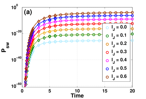
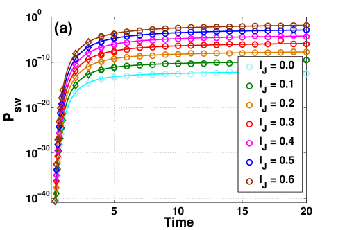
Figures 1 and 2 show the RSER as a function of time for seven values of $I_{J}$ between $0$ and $0.6$ with thermal stability factors $\Delta=60$ and $\Delta=30$, respectively. Runs at both temperatures are included here to facilitate comparison with the results presented in Ref. [6]. Both show a comparison between numerical solutions of backward FPE (24) and IS simulations for the macrospin model. For $T\geq 5$ in Fig. 1 and $T\geq 4$ in Fig. 2, infinite-time bias functions are used for IS while for $T\leq 6$ in Fig. 1 and $T\leq 5$ in Fig. 2, finite-time bias functions are used. Agreement between the FPE and IS results is excellent throughout the range of times and currents, and the IS results are internally consistent between the finite- and infinite-time bias functions used at $T=5$ and $T=6$ in Fig. 1, and used at $T=4$ in Fig. 2.

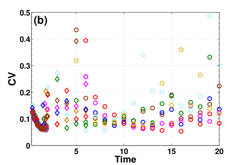
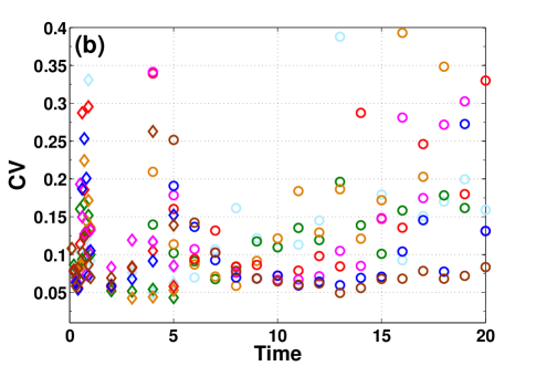
Fig. 1 (b) shows the CV for the IS estimates in Fig. 1 (a), and Fig. 2 (b) shows those for the estimates shown in Fig. 2 (a). The CV values for the IS estimates range from approximately $0.05$ to $0.5$. We note that with an inappropriate choice of bias the CV can be an imperfect measure of accuracy for Monte Carlo estimates using variance reduction [45]. However, this is precluded by our choice of an asymptotically optimal bias function that is based on large deviation theory [46, 24], as can also be seen from the excellent agreement with the solutions to FPE (24). The low CV values obtained for such extremely small probabilities with moderate sample size of $M=10^{3}$ are therefore a clear demonstration of the efficiency of the bias functions used here.

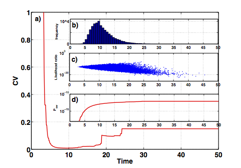
In both figures the CVs are observed to increase when $T$ is decreased from $T=10$ to $T=5$, indicating that the infinite-time bias function used for these runs becomes progressively less efficient at capturing the switching events as the time horizon shrinks. The application of finite-time bias functions for smaller times lowers the CVs as expected. Furthermore, Figs. 1 (b) and 2 (b) show a similar pattern in the CVs generated by IS with infinite-time bias functions, where the CVs also increase for large times $T$. Fig. 3 illustrates this sudden increase in CV in the context of longer times, as well as a histogram of switching times, and the time evolution of the spread in values of likelihood ratio.

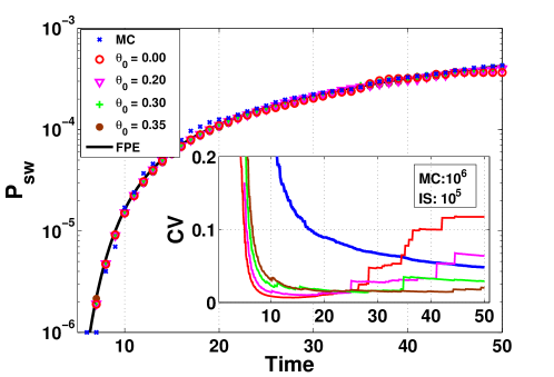
This decrease in efficiency of the infinite-time bias function for large but finite time horizons is due to the fact that exits have a natural finite time scale dictated by diffusion near the fixed points with the action minimizer bridging the gap between them. When the time horizon of the simulation is large relative to this time scale, it allows for exit events that hover near the stable fixed point before exiting just prior to the horizon time. These events occur with considerably higher likelihood under the unbiased dynamics than under the biased dynamics, leading to a very large likelihood ratio that causes them to dominate the CV computation. Since the diffusion time grows as the noise strength decreases, this phenomenon can be regarded as a finite-noise effect, and it indeed vanishes as $\Delta\to\infty$. We address this issue for finite noise by turning off the biasing near the stable fixed point, i.e., for $|\theta|<\theta_{0}$, with the results plotted for different values of $\theta_{0}$ in Fig. 4. It is clearly seen that as $\theta_{0}$ increases, the anomalous behavior for large horizon time is mitigated, at the expense of sampling efficiency for small horizon times.

Figure 3: CVs of IS estimators for $I_{J}=0.3$ with infinite-time bias functions and sample size $10^{5}$. Inset (a) is a histogram of exit times for the biased system. Inset (b) is the estimated likelihood ratio vs. time. Inset (c) is the probability of switching before time $T$. The sample size here is $M=10^{5}$.

IV-B Two coupled identical macrospins: model

To demonstrate that the IS method can also be effective in coupled systems, we simulate two spins with identical volume and dynamics given by (22), which in this case is explicitly

$$\dot{\theta}_{1} =c\sin(\theta_{2}-\theta_{1})+b(\theta_{1})+\sqrt{\frac{2}{{\Delta}}}\dot{W_{1}},$$ (32)

$$\dot{\theta}_{2} =c\sin(\theta_{1}-\theta_{2})+b(\theta_{2})+\sqrt{\frac{2}{{\Delta}}}\dot{W_{2}},$$ (33)

where $c>0$ is the ferromagnetic exchange coupling strength favoring parallel alignment of the two spins. The initial conditions are $\theta_{1}(0)=\theta_{2}(0)=0$. Recall that as a switching criterion we adopt that at least one of the angles reaches $\pi/2$ in absolute value.

Figure 4: Switching probabilities and CVs of IS estimators for $I_{J}=0.6$ with infinite-time bias functions active outside of a region containing the stable fixed point, defined by $\theta_{0}<|\theta|<\theta_{J}$, for different values of $\theta_{0}$. The sample size is $10^{5}$.

At finite temperature, the rare events of switching for the coupled spin system occur along the maximum likelihood paths, which are also the minimum energy paths of the system. When the system undergoes a transition, it switches by coherent rotation for strongly coupled spins, asymmetric coherent rotation for weakly coupled spins, or single particle reversal for extremely weakly coupled spin [47]. More precisely, in the limit of infinite coupling strength $c$, the coupled spin system collapses to the macrospin model with $\theta_{1}=\theta_{2}$, and the most probable path terminating at $\max(|\theta_{1}|,|\theta_{2}|)=\pi/2$ is identical to that of a single macrospin. As the coupling strength decreases, the dynamics of the coupled spin system changes significantly, ultimately leading to spins that evolve independently. Note that in $N$-dimensional coupled spin systems, the sequence of bifurcations from single macrospin dynamics to $N$-fold macrospin dynamics as $c$ decreases from infinity [48] further exacerbates the challenge in finding appropriate bias functions.

IV-C Two coupled identical macrospins: biased dynamics

The biased dynamics associated with (32) and (33) reads

$$\dot{\tilde{\theta}}_{1} =c\sin(\tilde{\theta}_{2}-\tilde{\theta}_{1})+b(\tilde{\theta}_{1})+\sqrt{2}\,u^{*}_{1}+\sqrt{\frac{2}{{\Delta}}}\dot{W_{1}},$$ (34)

$$\dot{\tilde{\theta}}_{2} =c\sin(\tilde{\theta}_{1}-\tilde{\theta}_{2})+b(\tilde{\theta}_{2})+\sqrt{2}\,u^{*}_{2}+\sqrt{\frac{2}{{\Delta}}}\dot{W_{2}}.$$ (35)

In contrast to the single macrospin case, for two coupled macrospins an exact analytical bias function is no longer available even for infinite-time biasing. Therefore, it is necessary to obtain numerical bias functions by minimizing the Freidlin-Wentzell action (9) with terminal condition $\max(|\theta_{1}(T_{sw})|,|\theta_{2}(T_{sw})|)=\pi/2$ for some $0<T_{sw}\leq T\leq\infty$.

For finite-time bias the action functional $S_{T}$ is given explicitly by

$$S_{T}[\theta_{1},\theta_{2}]=\frac{1}{4}\int_{t}^{T}\left(\dot{\theta}_{1}-c\sin(\theta_{2}-\theta_{1})-b(\theta_{1})\right)^{2}ds\\ +\frac{1}{4}\int_{t}^{T}\left(\dot{\theta}_{2}-c\sin(\theta_{1}-\theta_{2})-b(\theta_{2})\right)^{2}ds,$$ (36)

and the corresponding finite-time bias $(u^{*}_{1},u^{*}_{2})=(u^{*}_{T,1},u^{*}_{T,2})$ is

$$u^{*}_{T,1}(\tilde{\theta}_{1},\tilde{\theta}_{2},t)=\frac{1}{\sqrt{2}}(\dot{\theta}^{T}_{\tilde{\theta}_{1},\tilde{\theta}_{2},t,1}(t)-c\sin(\tilde{\theta}_{1}-\tilde{\theta}_{2})-b(\tilde{\theta}_{1})),$$ (37)

$$u^{*}_{T,2}(\tilde{\theta}_{1},\tilde{\theta}_{2},t)=\frac{1}{\sqrt{2}}(\dot{\theta}^{T}_{\tilde{\theta}_{1},\tilde{\theta}_{2},t,2}(t)-c\sin(\tilde{\theta}_{2}-\tilde{\theta}_{1})-b(\tilde{\theta}_{2})),$$ (38)

where $\theta^{T}_{\tilde{\theta}_{1},\tilde{\theta}_{2},t}(s)=(\theta^{T}_{\tilde{\theta}_{1},\tilde{\theta}_{2},t,1}(s),\theta^{T}_{\tilde{\theta}_{1},\tilde{\theta}_{2},t,2}(s))$ is the minimizer of $S_{T}$ satisfying $\theta^{T}_{\tilde{\theta}_{1},\tilde{\theta}_{2},t}(t)=(\tilde{\theta}_{1},\tilde{\theta}_{2})$ and $\max(|\theta^{T}_{\tilde{\theta}_{1},\tilde{\theta}_{2},t,1}(T)|,|\theta^{T}_{\tilde{\theta}_{1},\tilde{\theta}_{2},t,2}(T))|=\pi/2$.

For infinite-time bias, we minimize

$$S_{\infty}[\theta_{1},\theta_{2}]=\frac{1}{2}\int_{0}^{1}\biggl{(}\lambda(\theta_{1},\theta_{2})\sqrt{|\theta^{\prime}_{1}|^{2}+|\theta^{\prime}_{2}|^{2}}\\ -(c\sin(\theta_{2}-\theta_{1})+b(\theta_{1}))\theta_{1}^{\prime}-(c\sin(\theta_{1}-\theta_{2})+b(\theta_{2}))\theta_{2}^{\prime}\biggr{)}ds,$$ (39)

where

$$\lambda(\theta_{1},\theta_{2})=\Big{[}(c\sin(\theta_{2}-\theta_{1})\\ +b(\theta_{1}))^{2}+(c\sin(\theta_{1}-\theta_{2})+b(\theta_{2}))^{2}\Big{]}^{1/2},$$ (40)

and express the bias as

$$u^{*}_{\infty,1} (\tilde{\theta}_{1},\tilde{\theta}_{2})=\frac{1}{\sqrt{2}}$$

$$\times\left({\lambda(\tilde{\theta}_{1},\tilde{\theta}_{2})\theta^{\prime}_{\tilde{\theta}_{1},\tilde{\theta}_{2},1}(0)\over\sqrt{|\theta^{\prime}_{\tilde{\theta}_{1},\tilde{\theta}_{2},1}|^{2}+|\theta^{\prime}_{\tilde{\theta}_{1},\tilde{\theta}_{2},2}|^{2}}}-c\sin(\tilde{\theta}_{2}-\tilde{\theta}_{1})-b(\tilde{\theta}_{1})\right),$$ (41)

$$u^{*}_{\infty,2} (\tilde{\theta}_{1},\tilde{\theta}_{2})=\frac{1}{\sqrt{2}}$$

$$\times\left({\lambda(\tilde{\theta}_{1},\tilde{\theta}_{2})\theta^{\prime}_{\tilde{\theta}_{1},\tilde{\theta}_{2},2}(0)\over\sqrt{|\theta^{\prime}_{\tilde{\theta}_{1},\tilde{\theta}_{2},1}|^{2}+|\theta^{\prime}_{\tilde{\theta}_{1},\tilde{\theta}_{2},2}|^{2}}}-c\sin(\tilde{\theta}_{1}-\tilde{\theta}_{2})-b(\tilde{\theta}_{2})\right),$$ (42)

where $\theta_{\tilde{\theta}_{1},\tilde{\theta}_{2}}=(\theta_{\tilde{\theta}_{1},\tilde{\theta}_{2},1},\theta_{\tilde{\theta}_{1},\tilde{\theta}_{2},2})$ is the minimizer of $S_{\infty}$ with $\theta_{\tilde{\theta}_{1},\tilde{\theta}_{2},t}(0)=(\tilde{\theta}_{1},\tilde{\theta}_{2})$ and $\max(|\theta_{\tilde{\theta}_{1},\tilde{\theta}_{2},t,1}(1)|,|\theta_{\tilde{\theta}_{1},\tilde{\theta}_{2},t,2}(1))|=\pi/2$. Finally, the discretized version of the biased equations and the likelihood ratio are straightforward generalizations of (30) and (31).

Figure 5: IS estimate for switching probability (RSER) and CV of the RSER with sample size $M=10^{3}$ for a strongly coupled two-spin system. (a) RSER with applied currents ranging from $0$ to $0.6$ versus time $T$ with thermal stability factor $\Delta=60$ and coupling strength $c=0.8$. (b) CVs of IS estimates in (a). In both panels, open circles and open diamonds denote estimates generated by IS using infinite-time and finite-time bias functions, respectively. The colors correspond to different current amplitudes indicated in (a).

Figure 6: IS estimate for switching probability (RSER) and CV of the RSER with sample size $M=10^{3}$ for a weakly coupled two-spin system. (a) RSER with applied currents ranging from $0$ to $0.6$ versus time $T$ with thermal stability factor $\Delta=60$ and coupling strength $c=0.2$. (b) CVs of IS estimates in (a). In both panels, open circles and open diamonds denote estimates generated by IS using infinite-time and finite-time bias functions, respectively, and black dots denote estimates generated by naive MC simulations for $I_{J}=0.6$ with sample size $M=10^{5}$. The colors correspond to different current amplitudes indicated in (a).

Figure 7: Sample paths from IS for two-spin systems with current $I_{J}=0.1$ and thermal stability factor $\Delta=60$: strongly coupled spins with $c=0.8$ (a), weakly coupled spins with $c=0.2$ (b). False color corresponds to the effective potential in (23)

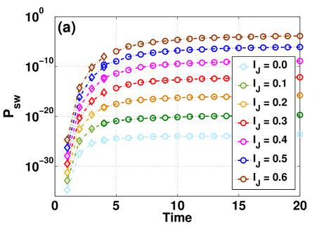
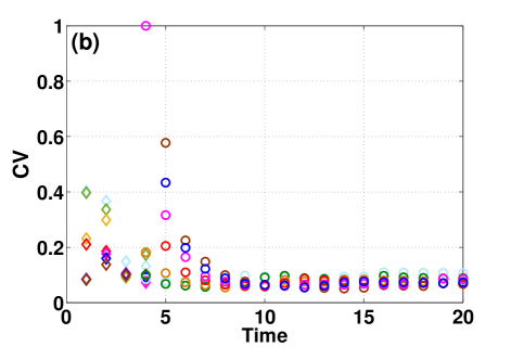
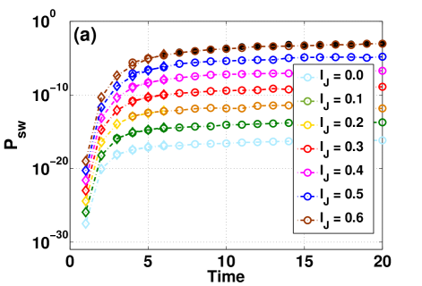
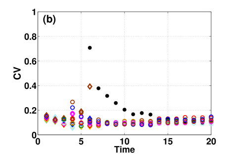
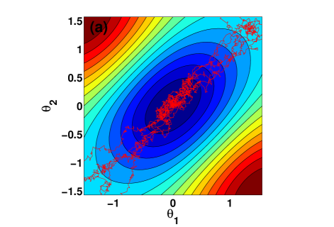
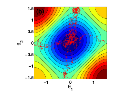
Fig. 5 (a) shows IS estimates of switching probabilities obtained using finite-time bias functions and infinite-time bias functions with a suitable cutoff near the origin applied to the coupled system with non-dimensional temperature $\Delta=60$ and coupling strength $c=0.8$. The coupling strength $c=0.8$ is an example of strong coupling, for which the spins rotate coherently along optimal switching paths. The open circles and open diamonds denote estimates generated by IS using infinite-time and finite-time bias functions, respectively. With sampling size of $M=10^{3}$, the infinite-time bias functions allow us to sample switching probabilities for $T\geq 5$ with $I_{J}$ ranging from $0$ to $0.6$. For $T\leq 4$, finite-time bias functions are used with IS. For infinite-time biasing the bias is switched off, i.e., $u^{*}_{\infty}$ is set to zero, when the effective potential from (23) of a configuration $(\tilde{\theta}_{1},\tilde{\theta}_{2})$ falls below that of $(\theta_{0},\theta_{0})$ with $\theta_{0}\in[0,0.3]$ chosen to minimize the CV.

Fig. 5 (b) shows the CVs becoming larger as time $T$ decreases, indicating that the infinite-time bias functions become less efficient. The effectiveness of using finite-time bias functions is evident in the CV values in Fig. 5 (b), where the CV values with open diamonds at time $T=4$ are much smaller than the CV values with open circles at times $T=4$ and $T=5$. This improved effectiveness comes with a cost of computing updated finite-time bias functions at each time step.

Similar results for a weakly coupled system are shown in Fig. 6. Fig. 6 (a) shows the switching probabilities as a function of time for different read currents with non-dimensional temperature $\Delta=60$ and coupling strength $c=0.2$. The coupling strength $c=0.2$ is an example of weak coupling, for which the spins rotate incoherently along optimal switching paths. With a sampling size of $M=10^{3}$, IS using infinite-time bias functions allows us to sample switching probabilities for $T\geq 4$ with $I_{J}$ ranging from $0$ to $0.6$. As in Fig. 5, Fig. 6 (b) shows a decrease in efficiency of IS using infinite-time bias functions as $T$ decreases.

Fig. 6 (a) also shows switching probabilities generated using naive MC simulations with a sample size of $M=10^{5}$ for read current $I_{J}=0.6$ at various pulse durations. Naive MC simulations at this sample size fail to accurately capture probabilities less than $10^{-5}$ while IS is able to estimate probabilities as low as $10^{-28}$. This is reflected in Fig. 6 (b) where the CV is seen to diverge as the probability estimate decreases. Finally, a few representative switching trajectories corresponding to the results in Figs. 5 and 6 are shown in Fig. 7.

Figure 8: CVs of estimates generated by IS (brown open circles) and naive MC (black dots) in Fig. 6.

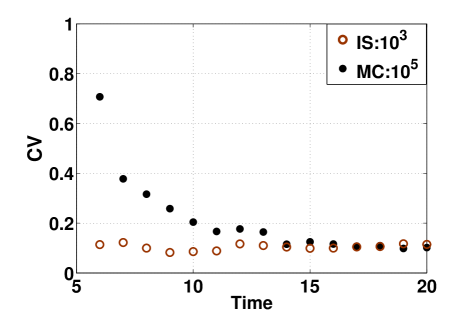
Fig. 8 shows a comparison between the CV for IS with sample size of $10^{3}$ and the CV for naive MC with sample size of $10^{5}$ for $I_{J}=0.6$. For time $6\leq T\leq 15$ the CVs for naive MC exceed the CVs for IS, by a factor ranging from 1 to 6 as the value of $T$ is decreased. This means that the number of IS samples required to achieve an estimate with the same or better accuracy than an estimate generated by naive MC is smaller by several orders of magnitude. For example, for switching probability by time $T=6$, where the CV ratio is about $6.2$, al least $3.8\times 10^{6}$ naive MC samples are required to achieve the same accuracy of an IS estimate generated using only $M=10^{3}$. This contrast is even more stark for smaller applied currents with much lower associated switching probabilities, where the computational effort required by naive MC simulations is prohibitive. Sampling-based probability estimates are only available using IS at these parameter values.

IV-D Failure to switch (WSER)

In this section, we estimate the WSER using MC and IS for both the macrospin model and two coupled-spin system, where the current is set sufficiently high as to drive the origin unstable, such that a switching event is expected to occur in the majority of random realizations. The two-spin state is considered to have switched when $\max(|\theta_{1}(T_{sw})|,|\theta_{2}(T_{sw})|)=\pi/2$ for some $0<T_{sw}\leq T.$

Figure 9: Non-switching probability as a function of time horizon for several values of the writing current, using thermal stability factor $\Delta=60$. The current $I_{J}$ is identified by color and ranges from 3 to 6. Solid lines denote numerical solutions of the backward Fokker-Planck equation for single macrospin, while dashed lines are simply visual guides. Filled circles denote IS estimates of the non-switching probabilities for a single macrospin. Open circles denote IS estimates of non-switching probabilities for two coupled spins with $c=0.2$.

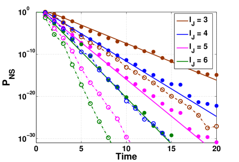
Fig. 9 shows a comparison between the numerical solution of the FPE and simulation results using IS for a single macrospin. Independent realizations of the macrospin evolution were computed with the same initial conditions, currents $I_{J}=3,4,5$, and $6$, and independent thermal noise with $\Delta=60$. The estimates obtained using $M=10^{4}$ IS samples show good agreement with the numerical solution of the backward FPE for moderate and long times. For the two-spin system, $10^{3}$ IS samples are used to estimate non-switching probabilities.

V Summary

In conclusion, we have applied IS to estimate error rates in reading and writing spin-torque memory devices in the macrospin limit and for the case of two coupled spins, using a variety of applied currents and thermal stability factors. We have demonstrated how IS is able to compute probabilities well below those computable using naive MC simulations, while producing accurate estimates with improved efficiency in cases where the probability is computable using naive MC but still very small. Depending on the time horizon of the read or write event relative to the drift dynamics of the spin system, IS simulations using infinite- or finite-time bias functions are appropriate. Infinite-time bias functions require only moderate computational cost; however, the increased cost can be significant in computing finite-time bias functions. Further improvement of the infinite-time biasing can be achieved by introducing a threshold turn the bias on only some distance away from the metastable equilibrium whose thermal stability is investigated.

In this appendix we derive a reduced model for the macrospin dynamics of the in-plane magnetization component in the regime of (19), which is done in the spirit of [36, 37, 38]. Our starting point is (13) for a macrospin $\mathbf{m}$, in which $\mathbf{h}$ satisfies (18). Introducing cylindrical coordinates, we can write

$$\mathbf{m}=\left(\sqrt{1-z^{2}}\,\cos\theta,\sqrt{1-z^{2}}\,\sin\theta,z\right).$$ (43)

Then, changing the unit of time to $\tau_{Q}$ we arrive, after some algebra and a change from Stratonovich to Itô formulation, to the following Itô SDEs for $\theta(t)$ and $z(t)$:

$${Q(1+\alpha^{2})\over\alpha}\dot{\theta} =-\frac{\partial E}{\partial z}-\frac{\alpha}{1-z^{2}}\frac{\partial E}{\partial\theta}+(a_{J}+\alpha b_{J})\frac{\sin\theta}{\sqrt{1-z^{2}}}$$

$$+(b_{J}-\alpha a_{J})\frac{z\cos\theta}{\sqrt{1-z^{2}}}+Q\sqrt{\frac{1+\alpha^{2}}{\Delta(1-z^{2})}}\,\dot{W_{1}},$$ (44)

$${Q(1+\alpha^{2})\over\alpha}\dot{z} =\frac{\partial E}{\partial\theta}-\alpha(1-z^{2})\frac{\partial E}{\partial z}-{Q\alpha z\over\Delta}$$

$$+(a_{J}+\alpha b_{J})z{\sqrt{1-z^{2}}}\,\cos\theta$$

$$-(b_{J}-\alpha a_{J})\sqrt{1-z^{2}}\,\sin\theta$$

$$+Q\sqrt{\Delta^{-1}(1+\alpha^{2})(1-z^{2})}\,\dot{W_{2}},$$ (45)

where $W_{1}$ and $W_{2}$ are two uncorrelated Brownian motions and

$$\frac{\partial E}{\partial z}=z-Qz\sin^{2}\theta,\quad\frac{\partial E}{\partial\theta}=Q(1-z^{2})\,\sin\theta\cos\theta.$$ (46)

We now assume that $Q\ll 1$, while $a_{J}=\beta^{-1}I_{J}Q$, $b_{J}=I_{J}Q$ and $\epsilon=Q/(2\Delta)$, with $I_{J}$, $\beta$ and $\Delta$ of order unity. In this case any deviations of $z$ from zero are strongly suppressed. Therefore, linearizing the above equations in $z$ and introducing $\zeta=Q^{-1}z$, we obtain

$${Q(1+\alpha^{2})\over\alpha}\dot{\theta} =-\frac{\partial E}{\partial z}-\alpha\frac{\partial E}{\partial\theta}+QI_{J}(\beta^{-1}+\alpha)\sin\theta$$

$$+Q^{2}I_{J}(1-\alpha\beta^{-1})\zeta\cos\theta$$

$$+Q\sqrt{\Delta^{-1}(1+\alpha^{2})}\,\dot{W_{1}},$$ (47)

$${Q^{2}(1+\alpha^{2})\over\alpha}\dot{\zeta} =\frac{\partial E}{\partial\theta}-\alpha\frac{\partial E}{\partial z}-{Q^{2}\alpha\zeta\over\Delta}$$

$$+Q^{2}I_{J}(\beta^{-1}+\alpha)\zeta\cos\theta$$

$$-QI_{J}(1-\alpha\beta^{-1})\sin\theta$$

$$+Q\sqrt{\Delta^{-1}(1+\alpha^{2})}\,\dot{W_{2}},$$ (48)

where

$$\frac{\partial E}{\partial z}=Q\zeta,\qquad\frac{\partial E}{\partial\theta}=Q\sin\theta\cos\theta.$$ (49)

Substituting (49) into (V) and (48), to the leading order in $Q\ll 1$ we then arrive at

$${(1+\alpha^{2})\over\alpha}\dot{\theta} =-\zeta-\alpha\sin\theta\cos\theta+I_{J}(\beta^{-1}+\alpha)\sin\theta$$

$$+\sqrt{\Delta^{-1}(1+\alpha^{2})}\,\dot{W_{1}},$$ (50)

$$0 =\sin\theta\cos\theta-\alpha\zeta-I_{J}(1-\alpha\beta^{-1})\sin\theta$$

$$+\sqrt{\Delta^{-1}(1+\alpha^{2})}\,\dot{W_{2}},$$ (51)

Finally, solving for $\zeta$ in (51) and substituting it back into (50), with the help of the fact that $\alpha W_{1}-W_{2}=\sqrt{1+\alpha^{2}}\,W$, where $W$ is another Brownian motion, we obtain (20). It is interesting to note that only the contribution of the field-like spin torque appears in the reduced equation, while the contribution of the Slonczewski torque cancels out to the leading order.

References

- [1] J.-G. Zhu, “Magnetoresistive random access memory: The path to competitiveness and scalability,” Proc. IEEE, vol. 96, pp. 1786 –1798, 2008.
- [2] A. V. Khvalkovskiy et al., “Basic principles of STT-MRAM cell operation in memory arrays,” J. Phys. D, vol. 46, p. 074001, 2013.
- [3] A. D. Kent and D. C. Worledge, “A new spin on magnetic memories,” Nature Nanotechnol., vol. 10, pp. 187–191, 2015.
- [4] D. Apalkov, B. Dieny, and J. M. Slaughter, “Magnetoresistive random access memory,” Proc. IEEE, vol. 104, pp. 1796–1830, 2016.
- [5] S. Bhatti, R. Sbiaa, A. Hirohata, H. Ohno, S. Fukami, and S. N. Piramanayagam, “Spintronics based random access memory: a review,” Materials Today, vol. 20, pp. 530–548, 2017.
- [6] W. H. Butler et al., “Switching distributions for perpendicular spin-torque devices within the macrospin approximation,” IEEE Trans. Magn., vol. 48, no. 12, pp. 4684–4700, Dec 2012.
- [7] Y. Xie, B. Behin-Aein, and A. W. Ghosh, “Fokker-Planck study of parameter dependence on write error slope in spin-torque switching,” IEEE Trans. Electron Devices, vol. 64, no. 1, pp. 319–324, Jan 2017.
- [8] M. Tzoufras, “Switching probability of all-perpendicular spin valve nanopillars,” AIP Advances, vol. 8, no. 5, p. 056002, 2018.
- [9] Y. Xie, J. Ma, S. Ganguly, and A. W. Ghosh, “From materials to systems: a multiscale analysis of nanomagnetic switching,” J Comput. Electron, vol. 16, pp. 1201–1226, 2017.
- [10] J. Z. Sun, R. P. Robertazzi, J. Nowak, P. L. Trouilloud, G. Hu, D. W. Abraham, M. C. Gaidis, S. L. Brown, E. J. O’Sullivan, W. J. Gallagher, and D. C. Worledge, “Effect of subvolume excitation and spin-torque efficiency on magnetic switching,” Phys. Rev. B, vol. 84, p. 064413, 2011.
- [11] R. Heindl, W. H. Rippard, S. E. Russek, M. R. Pufall, and A. B. Kos, “Validity of the thermal activation model for spin-transfer torque switching in magnetic tunnel junctions,” J. Appl. Phys., vol. 109, p. 073910, 2011.
- [12] H. Zhao et al., “Spin-torque driven switching probability density function asymmetry,” IEEE Trans. Magn., vol. 48, no. 11, pp. 3818–3820, Nov 2012.
- [13] Y. Shiota, T. Nozaki, S. Tamaru, K. Yakushiji, H. Kubota, A. Fukushima, S. Yuasa, and Y. Suzuki, “Evaluation of write error rate for voltage-driven dynamic magnetization switching in magnetic tunnel junctions with perpendicular magnetization,” Appl. Phys. Express, vol. 9, p. 013001, 2016.
- [14] D. Marcuse, “Derivation of analytical expressions for the bit-error probability in lightwave systems with optical amplifiers,” Journal of Lightwave Technology, vol. 8, pp. 1816–1823, 1990.
- [15] R. O. Moore, G. Biondini, and W. L. Kath, “A method to compute statistics of large, noise-induced perturbations of nonlinear Schrödinger solitons,” SIAM Review, vol. 50, p. 523, 2008.
- [16] D. P. Landau and K. Binder, A guide to Monte Carlo simulations in statistical physics. Cambridge ; New York: Cambridge University Press, 2000.
- [17] T. Dean and P. Dupuis, “Splitting for rare event simulation: A large deviation approach to design and analysis,” Stoch. Proc. Appl., vol. 119, no. 2, pp. 562 – 587, 2009.
- [18] R. Y. Rubinstein and D. P. Kroese, Simulation and the Monte Carlo method: Reuven Y. Rubinstein, Technion, Dirk P. Kroese, University of Queensland, 3rd ed., ser. Wiley series in probability and statistics. Hoboken, New Jersey: Wiley, 2017.
- [19] U. Roy, T. Pramanik, L. F. Register, and S. K. Banerjee, “Write error rate of spin-transfer-torque random access memory including micromagnetic effects using rare event enhancement,” IEEE Trans. Magn., vol. 52, no. 10, pp. 1–6, Oct 2016.
- [20] T. Pramanik, U. Roy, P. Jadaun, L. F. Register, and S. K. Banerjee, “Write error rates of in-plane spin-transfer-torque random access memory calculated from rare-event enhanced micromagnetic simulations,” J. Magn. Magn. Mater., vol. 467, pp. 96 – 107, 2018.
- [21] P. Dupuis and H. Kushner, “Stochastic systems with small noise, analysis and simulation; a phase locked loop example,” SIAM J. Appl. Math., vol. 47, no. 3, pp. 643–661, 1987.
- [22] G. Rubino and B. Tuffin, Rare Event Simulation Using Monte Carlo Methods. Wiley Publishing, 2009.
- [23] M. Cottrell, J.-C. Fort, and G. Malgouyres, “Large deviations and rare events in the study of stochastic algorithms,” Automatic Control, IEEE Transactions on, vol. 28, no. 9, pp. 907–920, 1983.
- [24] E. Vanden-Eijnden and J. Weare, “Rare event simulation of small noise diffusions,” Commun. Pure Appl. Math., vol. 65, no. 12, pp. 1770–1803, 12 2012.
- [25] M. I. Freidlin and A. D. Wentzell, Random Perturbations of Dynamical Systems. Berlin, Heidelberg: Springer Berlin Heidelberg, 2012.
- [26] P. Dupuis, K. Spiliopoulos, and H. Wang, “Importance Sampling for Multiscale Diffusions,” Multiscale Modeling & Simulation, vol. 10, no. 1, pp. 1–27, Jan. 2012. [Online]. Available: http://epubs.siam.org.libdb.njit.edu:8888/doi/abs/10.1137/110842545
- [27] M. Heymann and E. Vanden-Eijnden, “The geometric minimum action method: A least action principle on the space of curves,” Commun. Pure Appl. Math., vol. 61, no. 8, pp. 1052–1117, 2008.
- [28] C. J. García-Cervera, “Numerical micromagnetics: A review,” Bol. Soc. Esp. Mat. Apl., vol. 39, pp. 103—135, 2007.
- [29] A. Brataas, A. D. Kent, and H. Ohno, “Current-induced torques in magnetic materials,” Nature Mat., vol. 11, pp. 372–381, 2012.
- [30] G. Gioia and R. D. James, “Micromagnetics of very thin films,” Proc. R. Soc. Lond. Ser. A, vol. 453, pp. 213–223, 1997.
- [31] M. Hairer, “An introduction to stochastic PDEs,” arXiv:0907.4178, 2009.
- [32] W. F. Brown, “Thermal fluctuations of a single-domain particle,” Phys. Rev., vol. 130, pp. 1677–1686, 1963.
- [33] J. L. García-Palacios and F. J. Lázaro, “Langevin-dynamics study of the dynamical properties of small magnetic particles,” Phys. Rev. B, vol. 58, pp. 14 937–14 958, 1998.
- [34] D. Pinna, A. D. Kent, and D. L. Stein, “Spin-transfer torque magnetization reversal in uniaxial nanomagnets with thermal noise,” J. Appl. Phys., vol. 114, p. 033901, 2013.
- [35] K. A. Newhall and E. Vanden-Eijnden, “Averaged equation for energy diffusion on a graph reveals bifurcation diagram and thermally assisted reversal times in spin-torque driven nanomagnets,” J. Appl. Phys., vol. 113, no. 18, pp. 184 105–184 105–12, May 2013.
- [36] R. V. Kohn and V. Slastikov, “Effective dynamics for ferromagnetic thin films: a rigorous justification,” Proc. R. Soc. Lond. Ser. A, vol. 461, pp. 143–154, 2005.
- [37] C. J. Garcia-Cervera and W. E, “Effective dynamics for ferromagnetic thin films,” J. Appl. Phys., vol. 90, pp. 370–374, 2001.
- [38] R. G. Lund, G. D. Chaves-O’Flynn, A. D. Kent, and C. B. Muratov, “Reduced model for precessional switching of thin-film nanomagnets under the influence of spin torque,” Phys. Rev. B, vol. 94, p. 144425, Oct 2016.
- [39] J. Miles and B. Middleton, “A hierarchical micromagnetic model of longitudinal thin film recording media,” J. Magn. Magn. Mater., vol. 95, pp. 99–108, 1991.
- [40] J. J. Miles, M. Wdowin, J. Oakley, and B. K. Middleton, “The effect of cluster size on thin film media noise,” IEEE Trans. Magn., vol. 31, pp. 1013–1024, 1995.
- [41] J. Fidler and T. Schrefl, “Micromagnetic modelling—the current state of the art,” J. Phys. D: Appl. Phys., vol. 33, pp. R135–R156, 2000.
- [42] T. Taniguchi and H. Imamura, “Thermally assisted spin transfer torque switching in synthetic free layers,” Phys. Rev. B, vol. 83, p. 054432, 2011.
- [43] C. W. Gardiner, Handbook of stochastic methods for physics, chemistry and the natural sciences. Springer Series in Synergetics Springer-Verlag, 2004.
- [44] Y. Sun and X. Zhou, “An improved adaptive minimum action method for the calculation of transition path in non-gradient systems,” Commun. Comput. Phys., vol. 24, pp. 44–68, 2018.
- [45] P. Glasserman and Y. Wang, “Counterexamples in importance sampling for large deviations probabilities,” The Annals of Applied Probability, vol. 7, no. 3, pp. 731–746, Aug. 1997. [Online]. Available: https://projecteuclid.org/euclid.aoap/1034801251
- [46] P. Dupuis and H. Wang, “Subsolutions of an Isaacs equation and efficient schemes for importance sampling,” Mathematics of Operations Research, vol. 32, no. 3, p. 723, 2007.
- [47] W. Chen, S. Zhang, and N. H. Bertram, “Energy barriers for thermal reversal of interacting single domain particles,” J. Appl. Phys., vol. 71, no. 11, pp. 5579–5584, 1992.
- [48] N. Berglund, B. Fernandez, and B. Gentz, “Metastability in interacting nonlinear stochastic differential equations: I. From weak coupling to synchronization,” Nonlinearity, vol. 20, no. 11, p. 2551, 2007.