Semileptonic and nonleptonic decays of $D$ into tensor mesons with light-cone sum rule

S. Momeni e-mail: samira.momeni@phy.iut.ac.ir ā€ƒā€ƒ R. Khosravi e-mail: rezakhosravi @ cc.iut.ac.ir ā€ƒā€ƒ S. Ghaziasgar e-mail: sepide.ghaziasgar@ph.iut.ac.ir Department of Physics, Isfahan University of Technology, Isfahan 84156-83111, Iran
Abstract

Form factors of $D$ decays into $J^{PC}=2^{++}$ tensor mesons are calculated in the light-cone sum rules approach up to twist-4 distribution amplitudes of the tensor meson. The masses of the tensor mesons are comparable to that of the charm quark mass $m_{c}$; therefore all terms including powers of $m_{T}/m_{c}$ are kept out in the expansion of the two-particle distribution amplitude $\langle T|\bar{q}_{1\alpha}(x)\,q_{2\delta}(0)|0\rangle$. Branching ratios of the semileptonic $D\to T\,\mu\,\bar{\nu}_{\mu}$ decays and nonleptonic $D\to T~{}P~{}(P=K,\pi)$ decays are taken into consideration. A comparison is also made between our results and predictions of other methods and the existing experimental values for the nonleptonic case. The semileptonic branching ratios are typically of the order of $10^{-5}$, and the nonleptonic ones show better agreement with the experimental data in comparison to the Isgur-Scora-Grinstein-Wise predictions.

I Introduction

Analysis of heavy meson decays to the light ones, is a useful tool to explore the CKM matrix and $CP$ violations. The $D$- meson decays occurring by $c$ quark decay (in quark level) are placed in the above-mentioned processes.

In the semileptonic decays, the form factors determine the nonperturbative effects. The form factors of the semileptonic decays of charmed meson D(s)subscriptš·š‘ D_{(s)} to scalar, pseudoscalar or vector mesons have been estimated by various approaches. In Refs. Khodjamirian ; BallD , the light-cone sum rule (LCSR) approach has been used to study the $D\to\pi(K)\,\ell\,\nu$ decays. The form factors of the nonleptonic $D\to\pi(K,K^{*})\ell\,\nu$ transitions have been evaluated by the lattice QCD method in Ref. Abada ; Aubin ; Bernard , while the semileptonic processes $D\to\pi,\rho,K$ and $K^{*}$ have been investigated by the heavy quark effective theory in Ref. WangD . The semileptonic decays D(s)→f0​(K0āˆ—)​ℓ​ν→subscriptš·š‘ subscriptš‘“0superscriptsubscriptš¾0ā„“šœˆD_{(s)}\to f_{0}(K_{0}^{*})\,\ell\,\nu, D(s)→π​(K)​ℓ​ν→subscriptš·š‘ šœ‹š¾ā„“šœˆD_{(s)}\to\pi(K)\,\ell\,\nu, and D(s)→Kāˆ—ā€‹(ρ,Ļ•)​ℓ​ν→subscriptš·š‘ superscriptš¾šœŒitalic-Ļ•ā„“šœˆD_{(s)}\to K^{*}(\rho,\phi)\,\ell\,\nu have been studied in the framework of the three-point QCD sum rules (3PSR) Ignacio ; Aliev ; Ball2 ; Ball3 ; Ovchinnikov ; Baier90 ; Dong ; Mao . The $D$ meson decays into the axial vector meson, the Dq→K1​ℓ​ν​(q=u,d,s)→subscriptš·š‘žsubscriptš¾1ā„“šœˆš‘žš‘¢š‘‘š‘ D_{q}\to K_{1}\,\ell\,\nu\,(q=u,d,s) and $D\to\,a_{1},f_{1}(1285),f_{1}(1420)$ transitions are analyzed by the 3PSR approach Khosravi ; Zuo .

For the tensor meson, as the final state, the form factors have been calculated in the Isgur-Scora-Grinstein-Wise (ISGW) quark model and its improved version, the ISGW2 model in Refs. Isgur1989 ; Scora1995 . The observed $J^{PC}=2^{++}$ tensor mesons are: isovector meson $a_{2}(1320)$, isodoublet state $K_{2}^{*}(1430)$, and isosinglet mesons $f_{2}(1270)$ and $f_{2}^{\prime}(1525)$. $a_{2}(1320)$ is a $(d\bar{u})$ state, and $K_{2}(1430)$ is a (s​uĀÆ)š‘ ĀÆš‘¢(s\bar{u}) state, while the wave functions of $f_{2}$ and $f_{2}^{\prime}$ are defined as their mixing angle:

f2​(1270)=12​(u​uĀÆ+d​dĀÆ)​cos⁔θf2+s​s¯​sin⁔θf2,subscriptš‘“2127012š‘¢ĀÆš‘¢š‘‘ĀÆš‘‘subscriptšœƒsubscriptš‘“2š‘ ĀÆš‘ subscriptšœƒsubscriptš‘“2\displaystyle f_{2}(1270)=\frac{1}{\sqrt{2}}(u\bar{u}+d\bar{d})\cos\theta_{f_{2}}+s\bar{s}\sin\theta_{f_{2}},
f2′​(1525)=12​(u​uĀÆ+d​dĀÆ)​sin⁔θf2āˆ’s​s¯​cos⁔θf2.superscriptsubscriptš‘“2′152512š‘¢ĀÆš‘¢š‘‘ĀÆš‘‘subscriptšœƒsubscriptš‘“2š‘ ĀÆš‘ subscriptšœƒsubscriptš‘“2\displaystyle f_{2}^{\prime}(1525)=\frac{1}{\sqrt{2}}(u\bar{u}+d\bar{d})\sin\theta_{f_{2}}-s\bar{s}\cos\theta_{f_{2}}. (1)

Since $\pi\pi(KK)$ is the dominate decay of $f_{2}(f_{2}^{\prime})$ (for more information, see Hagiwara2002 ), the mixing angle should be small and it has been reported $\theta_{f_{2}}=7.8^{\circ}$ Li2001 and $\theta_{f_{2}}=(9\pm 1)^{\circ}$ Hagiwara2002 . Therefore, $f_{2}(1270)$ is primarily a $(u\bar{u}+d\bar{d})/\sqrt{2}$ state, while $f_{2}^{\prime}(1525)$ is dominantly (s​sĀÆ)š‘ ĀÆš‘ (s\bar{s}) Cheng2010 .

In this paper the form factors for the $D$ decays into light tensor mesons ($T$) in the LCSR approach are calculated. In this method, the operator product is expanded near the light cone, while the nonperturbative hadronic matrix elements are parametrized by the light-cone distribution amplitudes (LCDAs) of the tensor meson.

The paper is organized as follows: In Sec. II, by using the LCSR, the form factors of $D\to T\ell\bar{\nu}_{\ell}$ decays are derived. In Sec. III, the numerical analysis of the LCSR for the form factors is presented and the branching ratio values of the semileptonic and nonleptonic decays are evaluated. A comparison is also made between our results and the predictions of other methods and experimental data in this section.

II $D\to T$ form factors in the LCSR

In the LCSR method, to calculate the $D\to T$ transition form factors, first, the correlation function

Πμ​(p′,q)subscriptĪ šœ‡superscriptš‘ā€²š‘ž\displaystyle\Pi_{\mu}(p^{\prime},q) $\displaystyle=$ iā€‹āˆ«d4​x​ei​q​xā€‹āŸØT​(p′,Ī»)|š’Æā€‹{jμi​n​t​(x)​jD†​(0)}|0⟩,š‘–superscriptš‘‘4š‘„superscriptš‘’š‘–š‘žš‘„quantum-operator-productš‘‡superscriptš‘ā€²šœ†š’Æsuperscriptsubscriptš‘—šœ‡š‘–š‘›š‘”š‘„superscriptsubscriptš‘—š·ā€ 00\displaystyle i\int d^{4}xe^{iqx}\langle T(p^{\prime},\lambda)|{\cal{T}}\{j_{\mu}^{int}(x)\,j_{D}^{{\dagger}}(0)\}|0\rangle, (2)

where $j_{D}=i\bar{q}\gamma_{5}c$ is the interpolating current for the ${D}$ meson and q=u,sš‘žš‘¢š‘ q=u,s and $d$ for D=D0,Ds+š·superscriptš·0subscriptsuperscriptš·š‘ D=D^{0},D^{+}_{s} and $D^{+}$, respectively, is considered. Moreover, in Eq. (2), $j_{\mu}^{int}=\bar{q}^{\prime}\gamma_{\mu}(1-\gamma_{5})c$ is the interaction current in which $q^{\prime}=d$ for the $D^{0}\to a_{2}$ transition and q′=ssuperscriptš‘žā€²š‘ q^{\prime}=s for D0​(Ds+)→K2āˆ—ā€‹(f2′)→superscriptš·0superscriptsubscriptš·š‘ superscriptsubscriptš¾2superscriptsubscriptš‘“2′D^{0}(D_{s}^{+})\to K_{2}^{*}(f_{2}^{\prime}) decay. In addition, $\sqrt{2}\,j_{\mu}^{int}(D^{+}\to f_{2})=j_{\mu}^{int}(D^{0}\to a_{2}^{*})$.

According to the general philosophy of the LCSR, the correlation functions of Eq. (2) can be obtained in two ways: the physical or phenomenological side and the QCD or theoretical ones. The form factors can be obtained by using the dispersion relation to link these two parts.

Let us first consider the physical part of Eq. (2). By inserting a complete set of hadrons with the same quantum numbers of the $D$ meson between the currents and isolating the pole term of the lowest $D$ meson, correlation function is obtained as

Πμ​(p′,p)subscriptĪ šœ‡superscriptš‘ā€²š‘\displaystyle\Pi_{\mu}(p^{\prime},p) $\displaystyle=$ ⟨T​(p′,Ī»)|jμi​n​t​(x)|D​(p)āŸ©ā€‹āŸØD​(p)|jD†​(0)|0⟩mD2āˆ’p2+1Ļ€ā€‹āˆ«0āˆžĻĪ¼h​(s)sāˆ’p2ā€‹š‘‘s,quantum-operator-productš‘‡superscriptš‘ā€²šœ†superscriptsubscriptš‘—šœ‡š‘–š‘›š‘”š‘„š·š‘quantum-operator-productš·š‘superscriptsubscriptš‘—š·ā€ 00subscriptsuperscriptš‘š2š·superscriptš‘21šœ‹superscriptsubscript0superscriptsubscriptšœŒšœ‡ā„Žš‘ š‘ superscriptš‘2differential-dš‘ \displaystyle\frac{\langle T(p^{\prime},\lambda)|j_{\mu}^{int}(x)|D(p)\rangle\langle D(p)|j_{D}^{{\dagger}}(0)|0\rangle}{m^{2}_{D}-p^{2}}+\frac{1}{\pi}\int_{0}^{\infty}\frac{\rho_{\mu}^{h}(s)}{s-p^{2}}\,ds, (3)

where, the first term in Eq. (3) represents the ground-state $D$-meson contribution and the second term describes the contributions of the higher states and continuum, while $\rho_{\mu}^{h}$ is the spectral density for these states. These spectral densities are approximated by evoking the quark-hadron duality ansatz as

ρμh​(s)=ρμQ​C​D​(s)​θ​(sāˆ’s0),superscriptsubscriptšœŒšœ‡ā„Žš‘ superscriptsubscriptšœŒšœ‡š‘„š¶š·š‘ šœƒš‘ subscriptš‘ 0\displaystyle\rho_{\mu}^{h}(s)=\rho_{\mu}^{QCD}(s)\theta(s-s_{0}), (4)

where s0subscriptš‘ 0s_{0} is the continuum threshold chosen near the squared mass of the lowest $D$-meson state. It follows from Eq. (3) that to calculate the form factors of the $B\to T$ transition the matrix elements $\langle T(p^{\prime},\lambda)|j_{\mu}^{int}(x)|D(p)\rangle$ and ⟨D​(p)|jD†​(0)|0⟩quantum-operator-productš·š‘superscriptsubscriptš‘—š·ā€ 00\langle D(p)|j_{D}^{{\dagger}}(0)|0\rangle are needed. The first matrix element is defined in terms of the form factors as Hatanaka2009 ; Hatanaka2010 ; Wang2011

$\displaystyle\langle T(p^{\prime},\lambda)|j_{\mu}^{int}(x)|D(p)\rangle$ $\displaystyle=$ $\displaystyle-i{2V(q^{2})\over m_{D}+m_{T}}\epsilon_{\mu\nu\alpha\beta}\,e^{*\nu}_{\lambda}p^{\alpha}p^{\prime\beta}-A_{1}(q^{2})e_{\mu}^{*\lambda}(m_{D}+m_{T})+\frac{A_{2}(q^{2})}{m_{D}+m_{T}}(e^{*\lambda}.q)(p+p^{\prime})_{\mu}$ (5)
$\displaystyle+$ $\displaystyle 2m_{T}\frac{(e^{*\lambda}.q)}{q^{2}}q_{\mu}[A_{3}(q^{2})-A_{0}(q^{2})],$

with

$\displaystyle A_{3}(q^{2})=\frac{m_{D}+m_{T}}{2m_{T}}A_{1}(q^{2})-\frac{m_{D}-m_{T}}{2m_{T}}A_{2}(q^{2})~{}~{}~{}\rm{and}~{}~{}~{}~{}~{}~{}A_{3}(0)=A_{0}(0),$ (6)

where $q=p-p^{\prime}$, $e_{\mu}^{\lambda}=\varepsilon_{\mu\nu}^{\lambda}p^{\nu}/m_{D}$. Moreover, In Eq. (5), $V,A_{i}(i=0,..,3)$ are the form factors of $D\to T$ transition.

For simplicity, the following definitions are used:

$\displaystyle\mathcal{V}(q^{2})$ $\displaystyle=$ $\displaystyle-{2V(q^{2})\over m_{D}+m_{T}},~{}~{}~{}~{}~{}~{}~{}\mathcal{A}_{1}(q^{2})=-A_{1}(q^{2})(m_{D}+m_{T}),$
$\displaystyle\mathcal{A}_{2}(q^{2})$ $\displaystyle=$ $\displaystyle\frac{A_{2}(q^{2})}{m_{D}+m_{T}},~{}~{}~{}~{}~{}~{}~{}~{}~{}\mathcal{A}_{3}(q^{2})=\frac{2m_{T}}{q^{2}}[A_{3}(q^{2})-A_{0}(q^{2})].$ (7)

On the other hand, the second matrix element in Eq. (3) is defined in terms of the $D$-meson leptonic decay constant and mass as

⟨D​(p)|jD†​(0)|0⟩=fD​mD2mc+mq.quantum-operator-productš·š‘superscriptsubscriptš‘—š·ā€ 00subscriptš‘“š·superscriptsubscriptš‘šš·2subscriptš‘šš‘subscriptš‘šš‘ž\displaystyle\langle D(p)|j_{D}^{{\dagger}}(0)|0\rangle=\frac{f_{D}m_{D}^{2}}{m_{c}+m_{q}}. (8)

Using Eqs. (4), (5), (II) and (8), these hadronic representation can be obtained for Πμ​(p,p′)subscriptĪ šœ‡š‘superscriptš‘ā€²\Pi_{\mu}(p,p^{\prime}):

Πμ​(p′,p)subscriptĪ šœ‡superscriptš‘ā€²š‘\displaystyle\Pi_{\mu}(p^{\prime},p) $\displaystyle=$ $\displaystyle\frac{f_{D}m_{D}}{m_{c}+m_{q}}\frac{1}{m^{2}_{D}-p^{2}}\Bigg{\{}i\,\mathcal{V}(q^{2})\epsilon_{\mu\nu\alpha\beta}\,\varepsilon^{*\nu\rho}_{\lambda}p^{\alpha}p^{\prime\beta}p_{\rho}+\mathcal{A}_{1}(q^{2})\varepsilon_{\mu\sigma}^{*\lambda}p^{\sigma}+\mathcal{A}_{2}(q^{2})\varepsilon^{*\lambda}_{\alpha\beta}q^{\alpha}p^{\beta}(p+p^{\prime})_{\mu}$ (9)
$\displaystyle+$ $\displaystyle\mathcal{A}_{3}(q^{2})\varepsilon^{*\lambda}_{\alpha\beta}q^{\alpha}p^{\beta}q_{\mu}\Bigg{\}}+\frac{1}{\pi}\int_{s_{0}}^{\infty}\frac{\rho_{\mu}^{QCD}(s)}{s-p^{2}}\,ds.$

To obtain the theoretical part of Eq. (2) in the LCSR approach, the $\mathcal{T}$ product of currents should be expanded near the light cone $x^{2}\simeq 0$. After contracting the $c$ quark field,

Πμ​(p′,q)subscriptĪ šœ‡superscriptš‘ā€²š‘ž\displaystyle\Pi_{\mu}(p^{\prime},q) $\displaystyle=$ $\displaystyle-\int d^{4}xe^{iqx}\langle T(p^{\prime},\lambda)|\bar{q}^{\prime}(x)\gamma_{\mu}(1-\gamma_{5})\,S^{c}(x,0)\,\gamma_{5}\,\bar{q}(0)|0\rangle,$ (10)

where $S^{c}(x,0)$ is the full propagator of the $c$ quark, is obtained. In this paper, just the free propagator is considered as

$\displaystyle S^{c}(x,0)=\int\frac{d^{4}k}{(2\pi)^{4}}e^{-ikx}\frac{\not\!k+m_{c}}{k^{2}-m_{c}^{2}}.$ (11)

Using the Fierz rearrangement formula in Eq. (10), it follows that in order to calculate the theoretical part, the matrix elements of the nonlocal operators between $T$-meson and vacuum states are needed. Two-particle distribution amplitudes for the tensor meson $T$ are given in Yangt2011 ; Chengt2010 ,

$\displaystyle\langle T(p^{\prime},\lambda)|\bar{q}_{1\alpha}(x)\,q_{2\delta}(0)|0\rangle=-\frac{i}{4}\,\int_{0}^{1}du\,e^{iup^{\prime}x}\Bigg{\{}f_{T}m_{T}^{2}\Bigg{[}\not\!p^{\prime}\,\frac{\varepsilon^{*\lambda}_{\mu\nu}x^{\mu}x^{\nu}}{(p^{\prime}x)^{2}}\,\Phi^{T}_{\parallel}(u)-\not\!x{\varepsilon^{*\lambda}_{\mu\nu}x^{\mu}x^{\nu}\over 2(p^{\prime}x)^{3}}m_{T}^{2}\bar{g}_{3}^{T}(u)$
$\displaystyle\qquad+\left({\epsilon^{*\lambda}_{\mu\nu}x^{\nu}\over p^{\prime}x}-p^{\prime}_{\mu}{\varepsilon^{*\lambda}_{\nu\beta}x^{\nu}x^{\beta}\over(p^{\prime}x)^{2}}\right)\gamma^{\mu}\,g_{v}^{T}(u)+\frac{1}{2}\epsilon_{\mu\nu\rho\sigma}\gamma^{\mu}\varepsilon^{*\nu\beta}_{\lambda}x_{\beta}p^{\prime\rho}x^{\sigma}\gamma_{5}{1\over p^{\prime}x}\,g_{a}^{T}(u)\Bigg{]}$
$\displaystyle\qquad-\,{i\over 2}f^{\perp}_{T}m_{T}\Bigg{[}\frac{\sigma^{\mu\nu}\left(\varepsilon^{*\lambda}_{\mu\beta}x^{\beta}p^{\prime}_{\nu}-\varepsilon^{*\lambda}_{\nu\beta}x^{\beta}p^{\prime}_{\mu}\right)}{p^{\prime}x}\Phi^{T}_{\perp}(u)+\frac{\sigma^{\mu\nu}(p^{\prime}_{\mu}x_{\nu}-p^{\prime}_{\nu}x_{\mu})m_{T}^{2}\varepsilon^{*\lambda}_{\rho\beta}x^{\rho}x^{\beta}}{(p^{\prime}x)^{3}}\,\bar{h}_{t}^{T}(u)$
$\displaystyle\qquad+\sigma^{\mu\nu}\left(\varepsilon^{*\lambda}_{\mu\beta}x^{\beta}x_{\nu}-\varepsilon^{*\lambda}_{\nu\beta}x^{\beta}x_{\mu}\right)\frac{m_{T}^{2}}{2(p^{\prime}x)^{2}}\,\bar{h}_{3}^{T}(u)+\varepsilon^{*\lambda}_{\mu\nu}x^{\mu}x^{\nu}{m_{T}^{2}\over p^{\prime}x}\,h_{s}^{T}(u)\Bigg{]}+{\cal O}(x^{2})\Bigg{\}}_{\delta\alpha}\,,$ (12)

where $x^{2}\neq 0$ and

$\displaystyle\bar{g}_{3}(u)$ $\displaystyle=$ $\displaystyle{g}_{3}(u)+\Phi_{\parallel}(u)-2g_{v}(u),~{}~{}~{}~{}~{}\bar{h}_{t}(u)=h_{t}(u)-\frac{1}{2}\Phi_{\perp}(u),~{}~{}~{}~{}~{}\bar{h}_{3}(u)={h}_{3}(u)-\Phi_{\perp}(u).~{}~{}~{}~{}~{}$ (13)

In Eq. (II), $\Phi_{\parallel}$ and $\Phi_{\perp}$ are the twist-2 functions; $g_{v},g_{a},h_{t}$ and hssubscriptā„Žš‘ h_{s} are the twist-3 functions; ${g}_{3}$ and ${h}_{3}$ are of twist 4. The leading-twist $\Phi_{\parallel,\perp}$ can be expanded as Chengt2010

$\displaystyle\Phi_{(\parallel,\perp)}(u,\mu)=6u(1-u)\sum_{\ell=1}^{\infty}\,a^{\ell}_{(\parallel,\perp)}(\mu)C_{\ell}^{3/2}(\xi),$ (14)

and twist-3 LCDAs are related to twist-2 ones through the Wandzura-Wilczek relations:

$\displaystyle g_{v}(u)$ $\displaystyle=$ $\displaystyle\int_{0}^{u}dv\,\frac{\Phi_{\parallel}(v)}{\bar{v}}+\int_{u}^{1}dv\,\frac{\Phi_{\parallel}(v)}{v}\,,$
$\displaystyle g_{a}(u)$ $\displaystyle=$ $\displaystyle 2\bar{u}\int_{0}^{u}dv\,\frac{\Phi_{\parallel}(v)}{\bar{v}}+2u\int_{u}^{1}dv\,\frac{\Phi_{\parallel}(v)}{v}\,,$
$\displaystyle h_{t}(u)$ $\displaystyle=$ $\displaystyle\frac{3}{2}(2u-1)\left(\int_{0}^{u}dv\,\frac{\Phi_{\perp}(v)}{\bar{v}}-\int_{u}^{1}dv\,\frac{\Phi_{\perp}(v)}{v}\right)\,,$
hs​(u)subscriptā„Žš‘ š‘¢\displaystyle h_{s}(u) $\displaystyle=$ $\displaystyle 3\left(\bar{u}\int_{0}^{u}dv\,\frac{\Phi_{\perp}(v)}{\bar{v}}+u\int_{u}^{1}dv\,\frac{\Phi_{\perp}(v)}{v}\right)\,,$ (15)

where $\mu$ is the normalization scale, $\bar{u}=1-u$ and $\xi=2u-1$. Also, using the equation of motion given in Ref. Ball99 , we can express the twist-4 DAs.

Two-parton chiral-even light-cone distribution amplitudes of a tensor meson are given by

$\displaystyle\langle T(p^{\prime},\lambda)|\bar{q}_{1}(x)\gamma_{\mu}{q_{2}}(0)|0\rangle$ $\displaystyle=$ $\displaystyle f_{T}m^{2}_{T}\int\limits_{0}^{1}\!du\,e^{iup^{\prime}x}\Bigg{\{}p^{\prime}_{\mu}\frac{\varepsilon^{*\lambda}_{\alpha\beta}x^{\alpha}x^{\beta}}{(p^{\prime}x)^{2}}\,\Phi_{\parallel}^{T}(u)+\frac{\varepsilon^{*\lambda}_{\mu\alpha}x^{\alpha}}{p^{\prime}x}\,g_{v}^{T}(u)-\frac{m_{T}^{2}}{2}x_{\mu}\frac{\varepsilon^{*\lambda}_{\alpha\beta}x^{\alpha}x^{\beta}}{(p^{\prime}x)^{3}}\,g_{3}^{T}(u)\Bigg{\}}\,,$
$\displaystyle\langle T(p^{\prime},\lambda)|\bar{q}_{1}(x)\gamma_{\mu}\gamma_{5}q_{2}(0)|0\rangle$ $\displaystyle=$ $\displaystyle f_{T}m_{T}^{2}\int\limits_{0}^{1}\!du\,e^{iup^{\prime}x}\epsilon_{\mu\nu\alpha\beta}{x^{\nu}p^{\prime\alpha}}\varepsilon_{\lambda}^{*\beta\delta}x_{\delta}\,{g_{a}^{T}(u)\over p^{\prime}x}\,,$ (16)

and the chiral-odd LCDA is

$\displaystyle\langle T(p^{\prime},\lambda)|\bar{q}_{1}(x)\sigma_{\mu\nu}q_{2}(0)|0\rangle$ $\displaystyle=$ $\displaystyle-if_{T}^{\perp}m_{T}\int\limits_{0}^{1}\!du\,e^{iup^{\prime}x}\Bigg{\{}\left[\varepsilon^{*\lambda}_{\mu\alpha}x^{\alpha}p^{\prime}_{\nu}-\varepsilon^{*\lambda}_{\nu\alpha}x^{\alpha}p^{\prime}_{\mu}\right]\frac{1}{p^{\prime}x}\Phi_{\perp}^{T}(u)+(p^{\prime}_{\mu}x_{\nu}-p^{\prime}_{\nu}x_{\mu})$ (17)
$\displaystyle\times\frac{m_{T}^{2}\varepsilon^{*\lambda}_{\alpha\beta}x^{\alpha}x^{\beta}}{(p^{\prime}x)^{3}}h_{t}^{T}(u)+\frac{m_{T}^{2}}{2}\left[\varepsilon^{*\lambda}_{\mu\alpha}x^{\alpha}x_{\nu}-\varepsilon^{*\lambda}_{\nu\alpha}x^{\alpha}x_{\mu}\right]\frac{h_{3}^{T}(u)}{(p^{\prime}x)^{2}}\Bigg{\}}\,,$

where $f_{T}$ is scale independent, and $f_{T}^{\perp}$ is a scale-dependent decay constant of the tensor meson $T$, as defined in Ref. Chengt2010 .

Now, two-parton distribution amplitudes should be inserted in Eq. (10), and traces and integrals should be calculated. Finally, the same structures are equated both phenomenological and theoretical sides of the correlation functions, and the Borel transform is performed with respect to the variable $p^{2}$ as

$\displaystyle B_{p^{2}}(M^{2})\frac{1}{\left(p^{2}-m_{D}^{2}\right)^{n}}$ $\displaystyle=$ $\displaystyle\frac{(-1)^{n}}{\Gamma(n)}\frac{e^{-\frac{m_{D}^{2}}{M^{2}}}}{(M^{2})^{n}},$ (18)

the sum rules are obtained for the form factors describing $D\to T$ decay. For instance, the form factor $A_{1}(q^{2})$ is obtain as

$\displaystyle A_{1}(q^{2})$ $\displaystyle=$ $\displaystyle-\frac{\alpha_{1}}{m_{T}+m_{D}}\,\Bigg{\{}\frac{f_{T}^{\perp}}{m_{T}}\int_{u_{0}}^{1}du\,\frac{\Phi_{\perp}^{(i)T}}{8u^{2}}\Bigg{[}-31u+33\,(1+\frac{\delta_{1}(u)}{M^{2}})\Bigg{]}e^{-s(u)}-f_{T}^{\perp}m_{T}\int_{u_{0}}^{1}du\,\frac{\bar{h}_{3}^{(ii)T}}{u^{2}M^{2}}\Bigg{[}\frac{\delta_{2}(u)}{M^{2}}-\frac{1}{2}\Bigg{]}e^{-s(u)}$ (19)
$\displaystyle+$ 8​fTāŸ‚ā€‹mTā€‹āˆ«u01š‘‘u​ht(i​i​i)​Tu3​M2​[uāˆ’4+2​Γ1​(u)M2]​eāˆ’s​(u)+fT​mcā€‹āˆ«u01š‘‘u​[āˆ’gv(i)​T​(u)+12​ga(i)​T​(u)+8​mT2u​M2​gĀÆ3(i​i​i)​T]u2​M2​eāˆ’s​(u)8superscriptsubscriptš‘“š‘‡perpendicular-tosubscriptš‘šš‘‡superscriptsubscriptsubscriptš‘¢01differential-dš‘¢superscriptsubscriptā„Žš‘”š‘–š‘–š‘–š‘‡superscriptš‘¢3superscriptš‘€2delimited-[]š‘¢42subscriptš›æ1š‘¢superscriptš‘€2superscriptš‘’š‘ š‘¢subscriptš‘“š‘‡subscriptš‘šš‘superscriptsubscriptsubscriptš‘¢01differential-dš‘¢delimited-[]superscriptsubscriptš‘”š‘£š‘–š‘‡š‘¢12superscriptsubscriptš‘”š‘Žš‘–š‘‡š‘¢8superscriptsubscriptš‘šš‘‡2š‘¢superscriptš‘€2superscriptsubscriptĀÆš‘”3š‘–š‘–š‘–š‘‡superscriptš‘¢2superscriptš‘€2superscriptš‘’š‘ š‘¢\displaystyle 8\,f_{T}^{\perp}m_{T}\int_{u_{0}}^{1}du\frac{h_{t}^{(iii)T}}{u^{3}M^{2}}\Bigg{[}u-4+\frac{2\delta_{1}(u)}{M^{2}}\Bigg{]}e^{-s(u)}+f_{T}m_{c}\int_{u_{0}}^{1}du\frac{\left[-g_{v}^{(i)T}(u)+\frac{1}{2}g_{a}^{(i)T}(u)+8\frac{m_{T}^{2}}{uM^{2}}\bar{g}_{3}^{(iii)T}\right]}{u^{2}M^{2}}e^{-s(u)}
$\displaystyle+$ $\displaystyle f_{T}^{\perp}m_{T}\int_{u_{0}}^{1}du\,\frac{h_{s}^{(i)T}}{u^{2}M^{2}}e^{-s(u)}-f_{T}^{\perp}m_{T}\int_{u_{0}}^{1}du\,\frac{h_{3}^{(ii)T}}{u^{2}M^{2}}\Bigg{[}5+\frac{m_{c}^{2}}{u\,M^{2}}\Bigg{]}e^{-s(u)}\Bigg{\}},$

where

u0=12​mT2​[(s0āˆ’mT2āˆ’q2)2+4​mT2​(mc2āˆ’q2)āˆ’(s0āˆ’mT2āˆ’q2)],α1=mT2​(mc+mq)fD​mD​emD2M2,s​(u)=1u​M2​[mc2+u​u¯​mT2āˆ’u¯​q2],Ī“1​(u)=mc2u+mT2​u+q2​(uāˆ’2),Ī“2​(u)=mc2u+q2​uĀÆ2u,f(i)​(u)ā‰”āˆ«0uf​(v)ā€‹š‘‘v,f(i​i)​(u)ā‰”āˆ«0uš‘‘vā€‹āˆ«0vš‘‘Ļ‰ā€‹f​(ω),f(i​i​i)​(u)ā‰”āˆ«0uš‘‘vā€‹āˆ«0vš‘‘Ļ‰ā€‹āˆ«0Ļ‰š‘‘Ļ„ā€‹f​(Ļ„).subscriptš‘¢012superscriptsubscriptš‘šš‘‡2delimited-[]superscriptsubscriptš‘ 0superscriptsubscriptš‘šš‘‡2superscriptš‘ž224superscriptsubscriptš‘šš‘‡2superscriptsubscriptš‘šš‘2superscriptš‘ž2subscriptš‘ 0superscriptsubscriptš‘šš‘‡2superscriptš‘ž2missing-subexpressionsubscriptš›¼1superscriptsubscriptš‘šš‘‡2subscriptš‘šš‘subscriptš‘šš‘žsubscriptš‘“š·subscriptš‘šš·superscriptš‘’superscriptsubscriptš‘šš·2superscriptš‘€2š‘ š‘¢1š‘¢superscriptš‘€2delimited-[]superscriptsubscriptš‘šš‘2š‘¢ĀÆš‘¢superscriptsubscriptš‘šš‘‡2ĀÆš‘¢superscriptš‘ž2subscriptš›æ1š‘¢superscriptsubscriptš‘šš‘2š‘¢superscriptsubscriptš‘šš‘‡2š‘¢superscriptš‘ž2š‘¢2subscriptš›æ2š‘¢superscriptsubscriptš‘šš‘2š‘¢superscriptš‘ž2superscriptĀÆš‘¢2š‘¢superscriptš‘“š‘–š‘¢superscriptsubscript0š‘¢š‘“š‘£differential-dš‘£superscriptš‘“š‘–š‘–š‘¢superscriptsubscript0š‘¢differential-dš‘£superscriptsubscript0š‘£differential-dšœ”š‘“šœ”superscriptš‘“š‘–š‘–š‘–š‘¢superscriptsubscript0š‘¢differential-dš‘£superscriptsubscript0š‘£differential-dšœ”superscriptsubscript0šœ”differential-dšœš‘“šœmissing-subexpression\displaystyle\begin{array}[]{ll}u_{0}=\frac{1}{2\,m_{T}^{2}}\left[\sqrt{(s_{0}-m_{T}^{2}-q^{2})^{2}+4m_{T}^{2}(m_{c}^{2}-q^{2})}-\left(s_{0}-m_{T}^{2}-q^{2}\right)\right],&\\ \alpha_{1}=\frac{m_{T}^{2}~{}(m_{c}+m_{q})}{f_{D}\,m_{D}}\,e^{\frac{m_{D}^{2}}{M^{2}}},&s(u)=\frac{1}{u\,M^{2}}\left[m_{c}^{2}+u\,\bar{u}\,m_{T}^{2}-\bar{u}\,q^{2}\right],\\ \delta_{1}(u)=\frac{m_{c}^{2}}{u}+m_{T}^{2}\,u+q^{2}(u-2),&\delta_{2}(u)=\frac{m_{c}^{2}}{u}+q^{2}\frac{\bar{u}^{2}}{u},\\ {f}^{(i)}(u)\equiv\int_{0}^{u}f(v)dv,&{f}^{(ii)}(u)\equiv\int_{0}^{u}dv\int_{0}^{v}d\omega~{}f(\omega),\\ {f}^{(iii)}(u)\equiv\int_{0}^{u}dv\int_{0}^{v}d\omega~{}\int_{0}^{\omega}d\tau~{}f(\tau).\end{array}

The explicit expressions for the other form factors are presented in Appendix A.

III Numerical analysis

In this section, our numerical analysis of the sum rules for the form factors and branching ratios is presented. In the calculation of the form factors $V$ and $A_{i}(i=0,1,2)$, masses are taken in $\rm{GeV}$ as $m_{c}=1.28\pm 0.03$, $m_{{D}^{0}}=1.86$, $m_{{D}^{+}}=1.86$, mDs+=1.96subscriptš‘šsubscriptsuperscriptš·š‘ 1.96m_{{D}^{+}_{s}}=1.96 pdg . For the sš‘ s and $d$ quark at $\mu=1~{}\rm{GeV}$, we take $m_{d}=(3.5-6)~{}\rm{MeV}$ and $m_{d}=(104^{+26}_{-34})~{}\rm{MeV}$ Huang2004 . For $D^{0}$, $D^{+}$, and Dssubscriptš·š‘ D_{s}-meson decay constants, the results of the QCD sum rule as $f_{D^{0}}=f_{{D}^{+}}=(210.25\pm{11.60})~{}\mbox{MeV}$ and fDs=(245.70±7.46)​MeVsubscriptš‘“subscriptš·š‘ plus-or-minus245.707.46MeVf_{D_{s}}=(245.70\pm 7.46)~{}\mbox{MeV} Mutuk are used.

For the tensor mesons, the relevant parameters are presented in Table 1. All of the masses presented in Table 1 are chosen from Ref. pdg , while the decay constants $f_{T}(f_{T}^{\perp})$ and the Gegenbauer moments $a^{1}_{(\parallel,\perp)}$ are taken from Ref. Cheng2010 .

Table 1: Masses, decay constants and Gegenbauer moments for tensor mesons. The decay constants and Gegenbauer moments are given at the scale $\mu=1~{}\rm{GeV}$.
$T$ $a_{2}$ $K_{2}^{*}$ $f_{2}$ $f_{2}^{\prime}$
Mass (GeV) $1.32$ $1.42$ $1.27$ $1.52$
$f_{T}$ (MeV) $107\pm 6$ $118\pm 5$ $102\pm 6$ $126\pm 4$
$f_{T}^{\perp}$ (MeV) $105\pm 21$ $77\pm 14$ $117\pm 25$ $65\pm 12$
$a^{1}_{(\parallel,\perp)}$ $5/3$ $5/3$ $5/3$ $5/3$

III.1 Analysis of the form factors

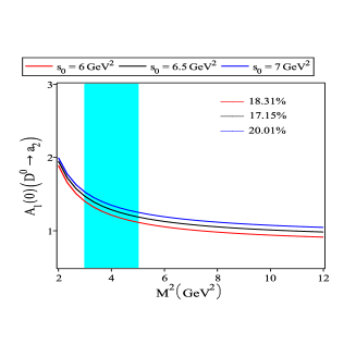
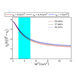
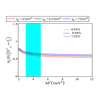
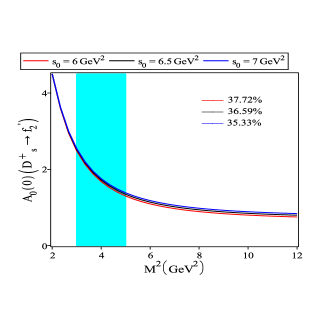
In this subsection, our numerical analysis of the form factors is presented. The sum rules for the form factors contain two parameters: namely, Borel mass squares $M^{2}$ and continuum thresholds s0subscriptš‘ 0s_{0}. Our results should be independent of these parameters since $M^{2}$ and s0subscriptš‘ 0s_{0} are not physical quantities. In this paper the value of continuum threshold is used as s0∈[6,8]​GeV2subscriptš‘ 068superscriptGeV2s_{0}\in[6,8]~{}\mbox{GeV}^{2} Khosravi . To carry out numerical calculations, a region of $M^{2}$ must be obtained and the suitable region has two conditions. First, the nonperturbative terms must remain subdominant by the lower bound of $M^{2}$; and second, the higher bound must decrease the contributions of the higher states and continuum. In Fig. 1, the $M^{2}$ dependence of the form factors $A_{1}(q^{2}=0)$ and $A_{0}(q^{2}=0)$ is presented for D0​(Ds+)→a2​(f2′)→superscriptš·0superscriptsubscriptš·š‘ subscriptš‘Ž2superscriptsubscriptš‘“2′D^{0}(D_{s}^{+})\to a_{2}(f_{2}^{\prime}) transition, at three different values of the threshold s0=6​GeV2subscriptš‘ 06superscriptGeV2s_{0}=6~{}\rm{GeV^{2}}, s0=6.5​GeV2subscriptš‘ 06.5superscriptGeV2s_{0}=6.5~{}\rm{GeV^{2}} and s0=7​GeV2subscriptš‘ 07superscriptGeV2s_{0}=7~{}\rm{GeV^{2}}, with red, black, and blue lines, respectively. In this figure, the relative change in the value of the form factors at $q^{2}=0$ is also displaced at the shaded interval of the Borel parameter. Our numerical analysis reveals that for $3~{}\rm{GeV^{2}}\leq M^{2}\leq 5~{}\rm{GeV^{2}}$ all of the form factors show good stability.

Refer to caption
Refer to caption
Refer to caption
Refer to caption
Figure 1: The form factors $A_{1}(0)$ and $A_{0}(0)$ for the D0​(Ds+)→a2​(f2′)→superscriptš·0superscriptsubscriptš·š‘ subscriptš‘Ž2superscriptsubscriptš‘“2′D^{0}(D_{s}^{+})\to a_{2}(f_{2}^{\prime}) transition on $M^{2}$ at three values of the threshold s0subscriptš‘ 0s_{{}_{0}}. The the relative change in the value of the form factors at the shaded interval of the Borel parameter is displaced in every plot.

Now, the $q^{2}$ dependency of the form factors can be carried out. First, the values of the form factors at $q^{2}=0$ are estimated. In Fig. 2, our results for ${V},{A}_{i}(i=0,1,2)$ of $D\to T\ell\bar{\nu}_{\ell}$ decays in $q^{2}=0$ are presented. Moreover, this table contains the predictions of the covariant light-front model (LFQM) and improved version ISGW quark model approaches Chengb ; Scora1995 . The results of the other approaches are rescaled according to Eq. (5). The errors in Fig. 2 are estimated by the variation of the Borel parameter $M^{2}$ and the decay constants $f_{T}$ and $f_{T}^{\perp}$.

Refer to caption
Refer to caption
Refer to caption
Refer to caption
Figure 2: The values of the ${V}(0),{A}_{i}(0)$ in comparison with the predictions of the other approaches, such as LFQM and ISGW.

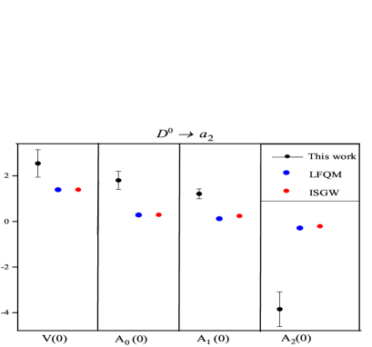
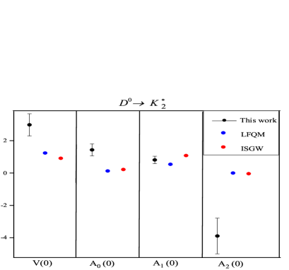
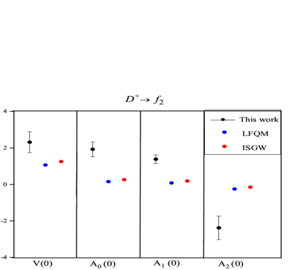
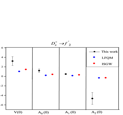
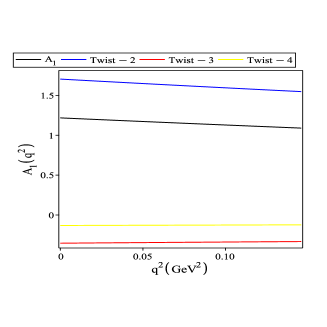
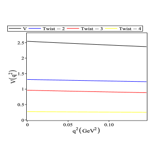
Figure 3 depicts the twist-2,3 and twist-4 contributions in the form factor formula $A_{1}(q^{2})$ and $V({q^{2}})$ for $D^{0}\to a_{2}$ decay. Similarity, as shown in this figure, for all of the form factors the most contribution is related to the twist-2 DAs, while the twist-4 DAs have the least contribution.

Refer to caption
Refer to caption
Figure 3: $A_{1}$ and $V$ form factor of $D^{0}\to a_{2}$ transition on $q^{2}$. The contributions of twist-2, 3 and twist-4 functions in these form factors are displaced with blue, red, and yellow lines, respectively.

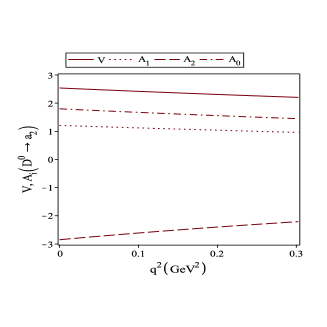
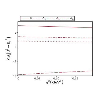
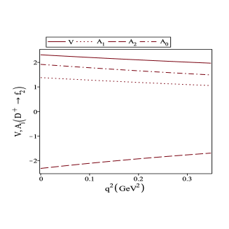
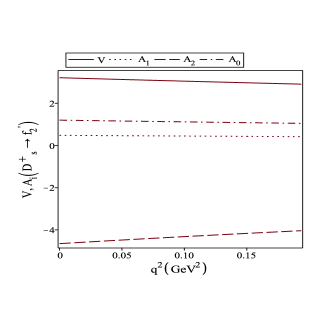
To extend the present result to the whole physical region, $m_{\ell}^{2}\leq q^{2}\leq(m_{D}-m_{T})^{2}$, we use the parametrization of the form factors with respect to $q^{2}$ as

$\displaystyle F(q^{2})=\frac{F(0)}{1+\alpha\,q^{2}/m_{D}^{2}+\beta\,q^{4}/m_{D}^{4}},$ (21)

where $F({0})$ denotes the value of the form factor at $q^{2}=0$. In addition, $\alpha$ and $\beta$ are the corresponding fitting coefficients listed in Table 2 for different form factors.

Table 2: The values of the parameter $F(0)$, $\alpha$, and $\beta$ for each form factor.
Form factor ${F(0)}$ $\alpha$ $\beta$ Form factor ${F(0)}$ $\alpha$ $\beta$
$V^{D^{0}\to a_{2}}$ ${2.54}$ $1.71$ $0.46$ $V^{D^{0}\to K^{*}_{2}}$ ${2.98}$ $1.80$ $0.58$
$A_{1}^{D^{0}\to a_{2}}$ ${1.21}$ $2.61$ $4.22$ $A_{1}^{D^{0}\to K^{*}_{2}}$ ${0.81}$ $2.60$ $4.43$
$A_{2}^{D^{0}\to a_{2}}$ ${-2.85}$ $3.12$ $2.75$ $A_{2}^{D^{0}\to K^{*}_{2}}$ ${-3.89}$ $2.77$ $1.81$
$A_{0}^{D^{0}\to a_{2}}$ ${1.80}$ $2.56$ $2.75$ $A_{0}^{D^{0}\to K^{*}_{2}}$ ${2.98}$ $1.80$ $0.58$
VDs+→f2′superscriptš‘‰ā†’subscriptsuperscriptš·š‘ superscriptsubscriptš‘“2′V^{D^{+}_{s}\to f_{2}^{\prime}} ${3.21}$ $2.04$ $0.81$ $V^{D^{+}\to f_{2}}$ ${2.31}$ $1.68$ $0.42$
A1Ds+→f2′superscriptsubscriptš“1→subscriptsuperscriptš·š‘ superscriptsubscriptš‘“2′A_{1}^{D^{+}_{s}\to f_{2}^{\prime}} ${0.48}$ $2.86$ $6.54$ $A_{1}^{D^{+}\to f_{2}}$ ${1.38}$ $2.62$ $4.14$
A2Ds+→f2′superscriptsubscriptš“2→subscriptsuperscriptš·š‘ superscriptsubscriptš‘“2′A_{2}^{D^{+}_{s}\to f_{2}^{\prime}} ${-4.65}$ $2.91$ $1.94$ $A_{2}^{D^{+}\to f_{2}}$ ${-2.32}$ $3.32$ $3.35$
A0Ds+→f2′superscriptsubscriptš“0→subscriptsuperscriptš·š‘ superscriptsubscriptš‘“2′A_{0}^{D^{+}_{s}\to f_{2}^{\prime}} ${1.20}$ $2.73$ $2.83$ $A_{0}^{D^{+}\to f_{2}}$ ${1.92}$ $2.58$ $2.85$

The dependence of the fitted form factors $V,A_{i}(i=0,1,2)$ on $q^{2}$ for $D\to T$ transitions is shown in Fig. 4.

Refer to caption
Refer to caption
Refer to caption
Refer to caption
Figure 4: The form factors $V,A_{i}$ on $q^{2}$ for $D\to T$ decay.

III.2 Differential branching ratio for the semileptonic decays

Now, we would like to evaluate the branching ratio values for the $D\to T\ell\bar{\nu}_{\ell}$ decays. The expressions of the differential decay width are given as

$\displaystyle\frac{d\Gamma_{L}(D\to T\ell\nu)}{dq^{2}}$ $\displaystyle=$ $\displaystyle\sigma\,\upsilon^{2}\,\left[\frac{1}{9}(2q^{2}+m_{\ell}^{2})h_{0}^{2}(q^{2})+\frac{1}{3}\lambda m_{\ell}^{2}A_{0}^{2}(q^{2})\right],$
$\displaystyle\frac{d\Gamma_{\pm}(D\to T\ell\nu)}{dq^{2}}$ $\displaystyle=$ $\displaystyle\sigma\,\upsilon^{2}\,\frac{(2q^{2}+m_{\ell}^{2})}{12}\Bigg{[}|(m_{D}+m_{T})A_{1}(q^{2})\mp\frac{\sqrt{\lambda}}{m_{D}+m_{T}}V(q^{2})|^{2}\Bigg{]},$ (22)

where $m_{\ell}$ represents the mass of the charged lepton and $L,\pm$ denotes the helicities of the tensor mesons. The other parameters are defined as

$\displaystyle\sigma$ $\displaystyle=$ $\displaystyle\frac{G_{F}^{2}\,|V_{q^{\prime}c}|^{2}\sqrt{\lambda^{3}(m_{D}^{2},m_{T}^{2},q^{2})}}{256~{}m_{D}^{5}~{}\,m_{T}^{2}~{}\pi^{3}q^{2}},~{}~{}~{}~{}~{}\upsilon=\left(1-\frac{m_{\ell}^{2}}{q^{2}}\right),$
$\displaystyle h_{0}(q^{2})$ $\displaystyle=$ $\displaystyle\frac{1}{2m_{T}}\left[(m_{D}^{2}-m_{T}^{2}-q^{2})(m_{D}+m_{T})A_{1}(q^{2})-\frac{\lambda}{m_{D}+m_{T}}A_{2}(q^{2})\right].$ (23)

The differential branching ratios of the $D\to T\,\mu\,\bar{\nu}_{\mu}$ decays are plotted on $q^{2}$ in Fig. 5, in which take $|V_{cd}|=(0.22\pm 0.00)$, |Vc​s|=(0.98±0.01)subscriptš‘‰š‘š‘ plus-or-minus0.980.01|V_{cs}|=(0.98\pm 0.01) and $m_{\mu}=105.65~{}\rm{MeV}$ pdg .

Refer to caption
Refer to caption
Refer to caption
Refer to caption
Figure 5: Differential branching ratios of the $D\to T\,\mu\,\bar{\nu}_{\mu}$ as functions of $q^{2}$.

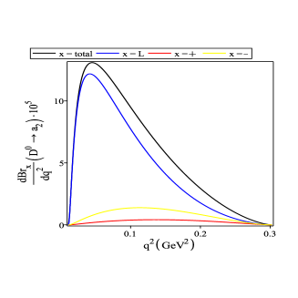
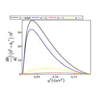
In this figure, the black, blue, red, and yellow lines show $dBr_{total}/dq^{2}$, $dBr_{L}/dq^{2}$, $dBr_{+}/dq^{2}$, and $dBr_{-}/dq^{2}$, respectively. Integrating Eq. (III.2) over $q^{2}$ in the whole physical region and using the total mean lifetime $\tau_{D^{0}}=0.41$, $\tau_{D^{+}}=1.04$ and, Ļ„Ds+=0.50subscriptšœsubscriptsuperscriptš·š‘ 0.50\tau_{D^{+}_{s}}=0.50 ps pdg , the branching ratio values of these decays are obtained as presented in Table 3.

Table 3: Branching ratios of $D\to T\,\mu\,\bar{\nu}_{\mu}$ obtained in this work. $\rm{Br}_{L}$, $\rm{Br}_{+}$, and $\rm{Br}_{-}$ stand for the portion of the rate with a longitudinal polarization, positive helicity, and negative helicity of the $T$-meson, respectively. The error comes from the variation of form factors.
Decay $[\rm{Br}_{L}$ $\rm{Br}_{+}$ $\rm{Br}_{-}$ $\rm{Br}_{total}]\times 10^{5}$
$D^{0}\to a_{2}\,\mu\,\bar{\nu}_{\mu}$ $1.23\pm 0.44$ $0.06\pm 0.01$ $0.21\pm 0.06$ $1.50\pm 0.51$
$D^{0}\to K_{2}^{*}\,\mu\,\bar{\nu}_{\mu}$ $2.35\pm 0.83$ $0.09\pm 0.03$ $0.41\pm 0.15$ $2.85\pm 1.01$
Ds+→f2′​μ​ν¯μ→subscriptsuperscriptš·š‘ superscriptsubscriptš‘“2ā€²šœ‡subscriptĀÆšœˆšœ‡D^{+}_{s}\to f_{2}^{\prime}\,\mu\,\bar{\nu}_{\mu} $1.52\pm 0.73$ $0.02\pm 0.01$ $0.22\pm 0.07$ $1.76\pm 0.81$
$D^{+}\to f_{2}\,\mu\,\bar{\nu}_{\mu}$ $6.37\pm 2.55$ $0.40\pm 0.19$ $1.08\pm 0.39$ $7.85\pm 3.13$

III.3 Nonleptonic decays

Finally, we want to evaluate the branching ratios for the nonleptonic $D\to T~{}P(P=K,\pi)$ decays. For these decays, the factorizable amplitude has the expression HCheng2003

$\displaystyle\mathcal{X}(D\to T~{}P)$ $\displaystyle=$ $\displaystyle i\frac{G_{F}}{\sqrt{2}}\,V_{cq^{\prime}}\,V_{uq_{{}_{2}}}^{*}\,f_{P}\,\varepsilon^{*}_{\mu\nu}\,p^{\mu}\,p^{\nu}\Bigg{[}\mathcal{A}_{1}(m^{2}_{P})+(m^{2}_{D}-m^{2}_{P})\,\mathcal{A}_{2}(m^{2}_{P})+m^{2}_{P}\,\mathcal{A}_{3}(m^{2}_{P})\Bigg{]}$ (24)
$\displaystyle=$ $\displaystyle\varepsilon^{*}_{\mu\nu}\,p^{\mu}\,p^{\nu}\,\mathcal{M}(D\to T~{}P),$

where q2=s​(d)subscriptš‘ž2š‘ š‘‘q_{2}=s~{}(d) for $P=K~{}(\pi)$. Also, $f_{P}$ is the $P$ meson decay constant, and $\mathcal{A}_{i}~{}~{}(i=1,2,3)$ is defined in Eq. (II). The decay rate is given by

$\displaystyle\Gamma(D\to T~{}P)=\frac{p_{c}^{5}}{12~{}\pi\,m_{T}^{2}}\left(\frac{m_{D}}{m_{T}}\right)^{2}\,|\mathcal{M}(D\to T~{}P)|^{2},$ (25)

where $p_{c}$ is the c.m. momentum of the tensor meson in the rest frame of the $D$ meson. For estimating the branching ratios of the nonleptonic $D\to T~{}P$ decays, the values of $\mathcal{A}_{i}~{}(i=1,2,3)$ at $q^{2}=m_{P}^{2}$ are needed. For $\pi$ and the $K$ meson, the masses are chosen in giga-electron-volts as $m_{\pi^{+}}=0.139$ and $m_{K^{+}}=0.493$ pdg . The results are presented in Table 4.

Table 4: The values of $\mathcal{A}_{i}(i=1,2,3)$ for $D\to T~{}P(P=K,\pi)$ transition at $q^{2}=m^{2}_{P}$.
$(D,T,P)$ $\mathcal{A}_{1}(m^{2}_{P})$ $\mathcal{A}_{2}(m^{2}_{P})$ $\mathcal{A}_{3}(m^{2}_{P})$
$(D^{0},a_{2},K^{+})$ $-3.85\pm 0.09$ $-0.88\pm 0.24$ $35.32\pm 39.07$
$(D^{0},K_{2}^{*},\pi^{+})$ $-2.61\pm 0.75$ $-1.16\pm 0.30$ $1.51\pm 23.05$
(Ds+,f2′,Ļ€+)subscriptsuperscriptš·š‘ superscriptsubscriptš‘“2′superscriptšœ‹(D^{+}_{s},f_{2}^{\prime},\pi^{+}) $-1.64\pm 0.31$ $-1.31\pm 0.34$ $3.41\pm 66.80$
(Ds+,f2′,K+)subscriptsuperscriptš·š‘ superscriptsubscriptš‘“2′superscriptš¾(D^{+}_{s},f_{2}^{\prime},K^{+}) $-1.39\pm 0.25$ $-1.21\pm 0.29$ $0.13\pm 4.54$
$(D^{+},f_{2},\pi^{+})$ $-4.25\pm 0.62$ $-0.72\pm 0.18$ $41.05\pm 37.29$

Inserting these values in Eq. (25) and using $|V_{ud}|=(0.97\pm 0.00)$, |Vu​s|=(0.22±0.00)subscriptš‘‰š‘¢š‘ plus-or-minus0.220.00|V_{us}|=(0.22\pm 0.00), $f_{\pi^{+}}=(130\pm 0.26)~{}\rm{MeV}$, and $f_{K^{+}}=(156\pm 0.49)~{}\rm{MeV}$, the values for the branching ratio of nonleptonic decays are obtained as presented in Table 5. In comparison, the experimental values and IGSW results are also included in this table. This table shows that for the $D^{0}\to a_{2}\,K^{+}$, $D^{0}\to K_{2}^{*}\,\pi^{+}$, and $D^{+}\to f_{2}\,\pi^{+}$ cases our results for the branching ratios are in good agrement with the experimental results.

Table 5: Branching ratios for various $D\to T~{}P(P=K,\pi)$ decays.
Decay IGSWHCheng2003 This work Exp E791 ; BaBar020 ; CLEO2002
Br$(D^{0}\to a_{2}\,K^{+})\times 10^{4}$ $0.05$ $7.06\pm 1.44$ $7.0\pm 4.3$
Br$(D^{0}\to K_{2}^{*}\,\pi^{+})\times 10^{3}$ $0.10$ $3.94\pm 0.54$ $2.0^{+1.3}_{-0.7}$
Br(Ds+→f2′​π+)Ɨ103→subscriptsuperscriptš·š‘ superscriptsubscriptš‘“2′superscriptšœ‹superscript103(D^{+}_{s}\to f_{2}^{\prime}\,\pi^{+})\times 10^{3} $1.6$ $4.58\pm 0.42$
Br(Ds+→f2′​K+)Ɨ106→subscriptsuperscriptš·š‘ superscriptsubscriptš‘“2′superscriptš¾superscript106(D^{+}_{s}\to f_{2}^{\prime}\,K^{+})\times 10^{6} $4.9$ $6.92\pm 2.94$
Br$(D^{+}\to f_{2}\,\pi^{+})\times 10^{3}$ $0.02$ $2.86\pm 0.68$ $0.9\pm 0.1$

In summary, the $D\to T\ell\bar{\nu}_{\ell}$ decays in the LCSR approach up to the twist-4 LCDAs of the $T$ tensor meson were considered. Using the transition form factors of the $D\to T$, the semileptonic branching ratios for $\ell=\mu$ and the nonleptonic ones for $D\to T~{}P(P=K,\pi)$ decay were analyzed. For the nonleptonic case, a comparison of the results for the branching ratios with the IGSW approach and existing experimental results was also made.

Appendix A Form Factor Expressions

In this Appendix, the explicit expressions for the form factors of $D\to T$ decays are given:

$\displaystyle V(q^{2})$ $\displaystyle=$ $\displaystyle\frac{\alpha_{1}}{2}{(m_{T}+m_{D})}\,\Bigg{\{}-f_{T}m_{c}\int_{u_{0}}^{1}du\,\frac{g_{a}^{(i)T}}{2u^{3}M^{4}}(2u+3)~{}e^{-s(u)}+\frac{1}{4}f_{T}\int_{u_{0}}^{1}du\,\frac{\Phi_{\perp}^{(i)T}}{u^{2}M^{2}}(2u-7)~{}e^{-s(u)}-8f_{T}^{\perp}m_{T}$
$\displaystyle\times\int_{u_{0}}^{1}du\,\frac{h_{t}^{(iii)T}}{u^{2}M^{4}}~{}e^{-s(u)}-\frac{1}{8}f_{T}^{\perp}m_{T}\int_{u_{0}}^{1}du\,\frac{\bar{h}_{t}^{(iii)T}}{u^{3}M^{4}}~{}(2u+1)~{}e^{-s(u)}-\frac{1}{2}f_{T}^{\perp}m_{T}\int_{u_{0}}^{1}du\,\frac{\bar{h}_{3}^{(ii)T}}{u^{2}M^{4}}~{}(u-1)~{}e^{-s(u)}$
$\displaystyle-$ $\displaystyle\frac{16}{3}\,f_{T}^{\perp}m_{T}\int_{u_{0}}^{1}du\,\frac{{h}_{3}^{(ii)T}}{u^{3}M^{4}}~{}(u-1)~{}e^{-s(u)}\Bigg{\}},$
$\displaystyle A_{2}(q^{2})$ $\displaystyle=$ $\displaystyle\alpha_{1}\,{(m_{T}+m_{D})}\,\Bigg{\{}f_{T}m_{c}\int_{u_{0}}^{1}du\frac{\left[9\,\Phi_{\|}^{(ii)T}-g_{v}^{(ii)T}+2\frac{m_{T}^{2}}{M^{2}}\bar{g}_{3}^{(iii)T}(u)\right]}{u^{3}\,M^{4}}\,~{}e^{-s(u)}-\frac{17f_{T}^{\perp}}{8m_{T}}\int_{u_{0}}^{1}du\frac{\Phi_{\perp}^{(i)T}}{u^{2}\,M^{2}}~{}e^{-s(u)}$
$\displaystyle+$ 2​fTāŸ‚ā€‹mTā€‹āˆ«u01š‘‘u​ht(i​i​i)​Tu3​M4​[39+4​uāˆ’24​Γ2​(u)M2+48​(1āˆ’Ī“1​(u)3​M2)]​eāˆ’s​(u)+12​fTāŸ‚ā€‹mTā€‹āˆ«u01š‘‘u​hs(i)​Tu2​M2​eāˆ’s​(u)2superscriptsubscriptš‘“š‘‡perpendicular-tosubscriptš‘šš‘‡superscriptsubscriptsubscriptš‘¢01differential-dš‘¢superscriptsubscriptā„Žš‘”š‘–š‘–š‘–š‘‡superscriptš‘¢3superscriptš‘€4delimited-[]394š‘¢24subscriptš›æ2š‘¢superscriptš‘€2481subscriptš›æ1š‘¢3superscriptš‘€2superscriptš‘’š‘ š‘¢12superscriptsubscriptš‘“š‘‡perpendicular-tosubscriptš‘šš‘‡superscriptsubscriptsubscriptš‘¢01differential-dš‘¢superscriptsubscriptā„Žš‘ š‘–š‘‡superscriptš‘¢2superscriptš‘€2superscriptš‘’š‘ š‘¢\displaystyle 2~{}f_{T}^{\perp}\,m_{T}\int_{u_{0}}^{1}du\frac{h_{t}^{(iii)T}}{u^{3}M^{4}}\Bigg{[}39+4u-24\,\frac{\delta_{2}(u)}{M^{2}}+48~{}(1-\frac{\delta_{1}(u)}{3M^{2}})\Bigg{]}~{}e^{-s(u)}+\frac{1}{2}f_{T}^{\perp}m_{T}\int_{u_{0}}^{1}du\,\frac{h_{s}^{(i)T}}{u^{2}M^{2}}~{}e^{-s(u)}
$\displaystyle-$ $\displaystyle\frac{1}{3}\,f_{T}\,m_{T}^{2}\,m_{c}\int_{u_{0}}^{1}du\,\frac{g_{3}^{(iii)T}}{u^{3}M^{6}}~{}e^{-s(u)}+2\,f_{T}^{\perp}m_{T}\int_{u_{0}}^{1}du\,\frac{h_{3}^{(ii)T}\,(2-u)}{u^{2}M^{4}}~{}e^{-s(u)}\Bigg{\}},$
$\displaystyle A_{0}(q^{2})$ $\displaystyle=$ $\displaystyle A_{3}(q^{2})-\frac{\alpha_{1}\,q^{2}}{2\,m_{T}}\Bigg{\{}f_{T}\,m_{c}\int_{u_{0}}^{1}du\frac{\left[-9\,\Phi_{\|}^{(ii)T}+g_{v}^{(ii)T}++(4-2u)\frac{m_{T}^{2}}{M^{2}}\,\bar{g}_{3}^{(iii)T}(u)\right]}{u^{3}\,M^{4}}\,~{}e^{-s(u)}+\frac{17f_{T}^{\perp}}{8m_{T}}$ (26)
$\displaystyle\times\int_{u_{0}}^{1}du\frac{\Phi_{\perp}^{(i)T}}{u^{2}\,M^{2}}~{}e^{-s(u)}+2~{}f_{T}^{\perp}\,m_{T}\int_{u_{0}}^{1}du\frac{h_{t}^{(iii)T}}{u^{3}M^{4}}\Bigg{[}-31-4u+24\,\frac{\delta_{2}(u)}{M^{2}}+48~{}(4-2u)\Bigg{]}~{}e^{-s(u)}$
$\displaystyle+$ 14​fTāŸ‚ā€‹mTā€‹āˆ«u01š‘‘u​hs(i)​Tu3​M4​(2āˆ’u)​[1āˆ’Ī“1​(u)3​M2]​eāˆ’s​(u)āˆ’16​fT​mT2​mcā€‹āˆ«u01š‘‘u​g3(i​i​i)​T​(2āˆ’u)u4​M6​eāˆ’s​(u)14superscriptsubscriptš‘“š‘‡perpendicular-tosubscriptš‘šš‘‡superscriptsubscriptsubscriptš‘¢01differential-dš‘¢superscriptsubscriptā„Žš‘ š‘–š‘‡superscriptš‘¢3superscriptš‘€42š‘¢delimited-[]1subscriptš›æ1š‘¢3superscriptš‘€2superscriptš‘’š‘ š‘¢16subscriptš‘“š‘‡superscriptsubscriptš‘šš‘‡2subscriptš‘šš‘superscriptsubscriptsubscriptš‘¢01differential-dš‘¢superscriptsubscriptš‘”3š‘–š‘–š‘–š‘‡2š‘¢superscriptš‘¢4superscriptš‘€6superscriptš‘’š‘ š‘¢\displaystyle\frac{1}{4}f_{T}^{\perp}m_{T}\int_{u_{0}}^{1}du\,\frac{h_{s}^{(i)T}}{u^{3}M^{4}}(2-u)\Bigg{[}1-\frac{\delta_{1}(u)}{3M^{2}}\Bigg{]}~{}e^{-s(u)}-\frac{1}{6}\,f_{T}\,m_{T}^{2}\,m_{c}\int_{u_{0}}^{1}du\,\frac{g_{3}^{(iii)T}\,(2-u)}{u^{4}M^{6}}~{}e^{-s(u)}
$\displaystyle+$ $\displaystyle 2\,f_{T}^{\perp}m_{T}\int_{u_{0}}^{1}du\,\frac{h_{3}^{(ii)T}\,(2-u)^{2}}{u^{3}M^{4}}~{}e^{-s(u)}\Bigg{\}}.$

References

  • (1) A. Khodjamirian, R. Ruckl, S. Weinzierl, C. Winhart, and O. I. Yakovlev, Phys.Rev. D 62, 114002 (2000).
  • (2) P. Ball, Phys. Lett. B 641, 50 (2006).
  • (3) A. Abada $et~{}al$. (SPQcdR Collaboration), Nucl. Phys. B, Proc. Suppl. 119, 625 (2003).
  • (4) C. Aubin $et~{}al$. (Fermilab Lattice Collaboration), Phys. Rev. Lett. 94, 011601 (2005).
  • (5) C. Bernard $et~{}al$., Phys. Rev. D 80, 034026 (2009).
  • (6) W. Y. Wang, Y. L. Wu, and M. Zhong, Phys. Rev. D 67, 014024 (2003).
  • (7) I. Bediaga and M. Nielsen, Phys. Rev. D 68, 036001 (2003).
  • (8) T. M. Aliev, V. L. Eletsky, and Ya. I. Kogan, Sov. J. Nucl. Phys. 40, 527 (1984).
  • (9) P. Ball, V. M. Braun, and H. G. Dosch, Phys. Rev. D 44, 3567 (1991).
  • (10) P. Ball, Phys. Rev. D 48, 3190 (1993).
  • (11) A. A. Ovchinnikov and V. A. Slobodenyuk, Z. Phys. C 44, 433 (1989).
  • (12) V. N. Baier and A. Grozin, Z. Phys. C 47, 669 (1990).
  • (13) D. S. Du, J. W. Li, and M. Z. Yang, Eur. Phys. J. C 37, 137 (2004).
  • (14) M. Z. Yang, Phys. Rev. D 73, 034027 (2006).
  • (15) R. Khosravi, K. Azizi, and N. Ghahramany, Phys. Rev. D 79, 036004 (2009).
  • (16) Y. Zuo $et~{}al$, Int. J. Mod. Phys. A 31, 1650116 (2016).
  • (17) N. Isgur, D. Scora, B. Grinstein, and M.B. Wise, Phys. Rev. D 39, 799 (1989).
  • (18) D. Scora and N. Isgur, Phys. Rev. D 52, 2783 (1995).
  • (19) K. Hagiwara $et~{}al$. (Particle Data Group) Phys. Rev. D 66, 010001 (2002).
  • (20) D. M. Li, H. Yu, and Q. X. Shen, J. Phys. G 27, 807 (2001).
  • (21) H. Y. Cheng, Y. Koike, and K. C. Yang, Phys. Rev. D 82, 054019 (2010).
  • (22) H. Hatanaka and K. C. Yang, Phys. Rev. D 79, 114008 (2009).
  • (23) H. Hatanaka and K. C. Yang, Eur. Phys. J. C 67, 149 (2010).
  • (24) W. Wang, Phys. Rev. D 83, 014008 (2011).
  • (25) K. Yang, Phys. Lett. B 695, 444 (2011).
  • (26) H. Cheng, Y. Koike, and K. Yang, Phys. Rev. D 82, 054019 (2010).
  • (27) P. Ball and V. M. Braun, Nucl. Phys. B 543, 201 (1999).
  • (28) K. A. Olive $et~{}al$. (Particle Data Group), Chin. Phys. C 38, 090001 (2014) and (2015) update.
  • (29) M. Q. Huang, Phys. Rev. C 69, 114015 (2004).
  • (30) H. Mutuk, Adv. High Energy Phys. 2018, 8095653 (2018).
  • (31) H.Y. Cheng, C.K. Chua, and C.W. Hwang, Phys. Rev. D 69, 074025 (2004).
  • (32) H. Y. Cheng, Phy. Rev. D 68, 014015 (2003).
  • (33) E. M. Aitala $et~{}al$. (E791 Collaboration), Phys. Rev. Lett. 89, 121801 (2002).
  • (34) B. Aubert $et~{}al$. (BABAr Collaboration), arxiv: hep-ex /0207089.
  • (35) H. Muramatsu $et~{}al$. (CLEO Collaboration), Phys. Rev. Lett. 89, 251802 (2002).