SUMMARIZATION AND VISUALIZATION OF LARGE VOLUMES OF BROADCAST VIDEO DATA

A report submitted in partial fulfillment of

the requirements for the degree of

Bachelor of Technology

by

Kumar Abhishek
and
Yogi Ashok Sunil

Under the guidance of
Dr. Prithwijit Guha

DEPARTMENT OF ELECTRONICS

& ELECTRICAL ENGINEERING

INDIAN INSTITUTE OF TECHNOLOGY GUWAHATI

April 2015

This is to certify that the work contained in this project report entitled “Summarization and Visualization of Large Volumes of Broadcast Video Data" submitted by Kumar Abhishek and Yogi Ashok Sunil to Department of Electronics and Electrical Engineering, Indian Institute of Technology Guwahati under my supervision and that it has not been submitted elsewhere for a degree.

Guwahati - 781 039 Dr. Prithwijit Guha
$22^{\text{nd}}$ April, 2015 (Assistant Professor, EEE Dept.)

ACKNOWLEDGEMENT

We would like to express our deepest appreciation to our thesis supervisor, Dr. Prithwijit Guha who constantly motivated us to work in this direction and valued our ideas. We would like to thank him for the freedom he gave us to carry out research in the field of our interest. We are indebted to Mr. Raghvendra Kannao for the constant support and technical help. We would also like to thank Mr. Rajul Gupta and Mr. Rajesh Ratnakaram for their valuable suggestions. Finally, we would like to thank our parents and friends for their immense love and support during our entire student life.

ABSTRACT

Over the past few years there has been an astounding growth in the number of news channels as well as the amount of broadcast news video data. As a result, it is imperative that automated methods need to be developed in order to effectively summarize and store this voluminous data. Format detection of news videos plays an important role in news video analysis. Our problem involves building a robust and versatile news format detector, which identifies the different band elements in a news frame. Probabilistic progressive Hough transform has been used for the detection of band edges. The detected bands are classified as natural images, computer generated graphics (non-text) and text bands. A contrast based text detector has been used to identify the text regions from news frames. Two classifers have been trained and evaluated for the labeling of the detected bands as natural or artificial - Support Vector Machine (SVM) Classifer with RBF kernel, and Extreme Learning Machine (ELM) classifier. The classifiers have been trained on a dataset of $6000$ images ($3000$ images of each class). The ELM classifier reports a balanced accuracy of $77.38$%, while the SVM classifier outperforms it with a balanced accuracy of $96.5$% using $10$-fold cross-validation. The detected bands which have been fragmented due to the presence of gradients in the image have been merged using a three-tier hierarchical reasoning model. The bands were detected with a Jaccard Index of $0.8138$, when compared to manually marked ground truth data. We have also presented an extensive literature review of previous work done towards news videos format detection, element band classification, and associative reasoning.

Chapter 1 Introduction

Classification of broadcast news videos is the first step towards news content analytics and understanding. The exponentially increasing amount of digital news broadcast videos makes it practically impossible to manually classify the news videos. This demands for an automatic and efficient method of classifying news videos. Various techniques of classifying and analyzing the news videos had been proposed in the past [1][2]. Most of these methods use prior knowledge about the news format and hence fails to classify the videos whose format is unknown.
Format detection is the detection of relevant element bands from a video frame viz. anchor shot, field shot, news ticker, channel logo, news headline etc. and create a format profile using these bands. Arguably, format detection is a precursor for any video content analysis and hence the result of format detection directly affects the efficiency of further video analysis and classification.

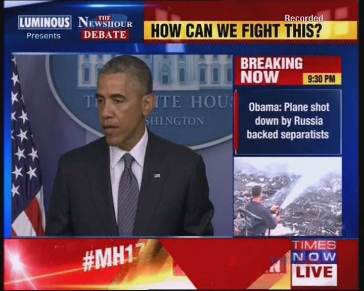
((a))

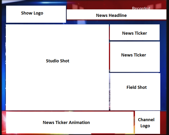
((b))

Figure 1.1: Example of news format detection for “The Newshour Debate" show (a) Original news video frame (b) Expected output format of the news video frame.

1.1 Motivation

Multimedia streaming requires a large bandwidth, especially if the content being transmitted is of very high quality. One page of text can require 500 to 1000 bytes [3] while a single full screen image may require 3,00,000 to 10,00,000 bytes [4]. These figures indicate that text can be transferred very effectively compared to the images. Hence, transmitting machine-encoded news ticker text instead of the text image can remarkably reduce the bandwidth requirement. Most of the news video frame comprises of individual element bands. Dynamic bands are the ones which gets changed in each frame while static bands are the ones which are constant for a specific time interval Fig. 1.2. Transmission of only the dynamic bands in the news video can help in further lowering the bandwidth requirement.

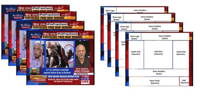
Figure 1.2: Video frame shots illustrating Dynamic and Static bands.

Storage requirement is another constraint which could be reduced by storing only the relevant bands from the video. Detection of irrelevant bands like advertisement ticker and images could be done after detecting the profile format and these bands can then be eliminated while storing the news videos for future reference. Finally, format detection can also play an important role in automatic censoring of the videos.

1.2 Proposed Approach

In this project we aim to build a robust news format detector which can accurately split a news video frame into different element bands and create a format profile using these bands.

Fig. 1.3 summarizes the format detection scheme. Firstly, Hough Transform has been used to detect lines from the video frame. The Hough lines are then extended to the frame boundaries and all the intersection point of the lines are used to generate low-level rectangles. A contrast based text detector [5] is used to detect the text bands and a SVM classifier is used to classify the natural and artificial bands. The similar low-level rectangular bands are further merged using the classifier’s output to generate the final high-level bands. Finally, these bands are combined together using three-tier associative reasoning to form a format profile.

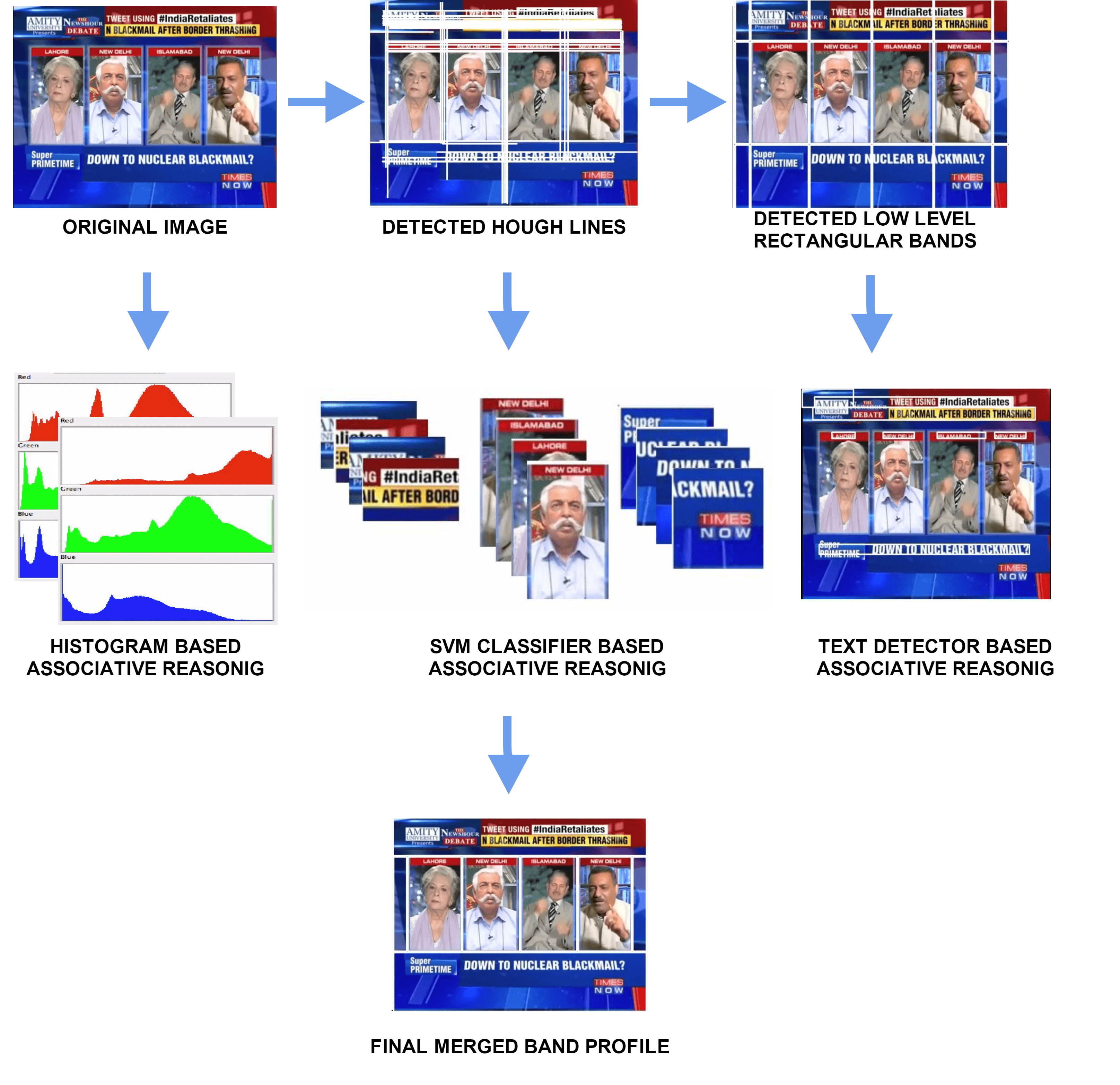
Figure 1.3: Illustrating the proposed approach for news video format detection.

1.3 Outline

The next chapter throws light on the extensive literature review on the methods of news format detection and band classification. In Chapter $3$, we describe the generation of lines using Hough transform and the formation of rectangular bands. Chapter $4$ describes the text-detector for detecting the text regions in the image. In Chapter $5$, we discuss the features used for designing the band classifier. Chapter $6$ elaborates the efficiency of the two classifiers used. In Chapter $7$, we propose a change detection based approach to detect the band type. Chapter $8$ discusses the three-tier reasoning model used for merging the low-level bands. In Chapter $9$ we have mentioned the accuracy of various sub-models and the overall approach. Chapter $10$ concludes the report. Chapter $11$ presents the future work. An Appendix at the end briefly describes the data marking tools created for generating the ground truth data and the training data.

Chapter 2 Literature Review

This chapter discusses the literature that provides with the work that has been done related with this project. Literature review is divided into two parts, namely, Element Band Detection and Element Band Classification.

2.1 Element Band Detection

Most of the work in the field of news video analytics and summarization is based on prior knowledge of the video format [6][7]. In some of the news video analysis method [8][9], video frames as a whole are directly used for analyzing the videos without dividing it into different format bands. Zhang et al. [10] proposed a method for frame detection to be used in automatic parsing of news video. However, the approach required comparing the video frames with pre-defined news format models and classifying it based on the nearest match. As this method is based on the prior knowledge of the format of news show and news channel, it fails to detect the format in cases where the apriori information is unavailable.
Hence, to the best of our knowledge, no previous work has been done in detecting the format of unknown news video and without considering any prior knowledge.

2.2 Element Band Classification

Previous work done to classify images has been primarily with an aim to index the images on the web for search engine optimization (SEO) of web image search.

Vassilis Athitsos, Michael J. Swain, and Charles Frankel worked on the classification of images into photographs and graphics on the World Wide Web [11]. The designed classifier was used by WebSeer [12], an image search engine. The features incorporated were total number of different colors, the fraction of pixels having the prevalent color, farthest neighbor metric, the fraction of pixels with a saturation greater than a certain threshold, color histogram metric, farthest neighbor histogram metric, dimension ratio metric and smallest dimension metric. Multiple binary decision trees [13] were used for classification and the reported accuracy was 91.4% on a dataset comprising of 9833 graphics and 1733 photographs.

Jing Huang et al. introduced a new feature known as “color correlogram” for the purposes of image indexing and comparison [14]. Ever since, color correlograms have been used widely used for the image classification, amongst other purposes. The correlogram is a robust feature and is used to utilize the information from the spatial correlation of colors in an image.

Rainer Lienhart and Alexander Hartmann worked on heirarchical classification of images [15] on the web into 2 broad categories, and then each category was divided into two sub- categories. Images were classified as photographs and graphical images. The photographs were then categorized into actual photographs and artificial, but photo-like images. The graphical images were categorized into presentation slides/scientific posters and comics/cartoons. The features considered for classification were total number of different colors after representing each color channel by only 5 bits (32768 colors), the prevalent color, fraction of pixels ($f_{1}$) from the farthest neighbor metric having a distance greater than zero, fraction of pixels ($f_{2}$) with a distance greater than some chosen higher threshold, and the ratio $\dfrac{f_{2}}{f_{1}}$. These features were trained on 7516 images using Adaboost algorithm, and the algorithm achieved an accuracy of 97.69%.

Yuanhao Chen et al. worked on the classification of images into photographs and graphics for the purpose of web image search as well as personal photograph management [16]. The features used were ranked histogram, color moments (mean, standard deviation and skewness) in the HSV color space [17], color correlogram [14], farthest neighbor histogram [11] and the relative size of the largest region and/or the number of regions of color constancy (or within a certain tolerance threshold) with a relative size bigger than a certain threshold. Adaboost learning algorithm was used as the classifier, and it was trained over a dataset of 36000 graphics and 35000 natural images. Five-fold cross validation [18] was used to validate the algorithm and an accuracy of 94.5% was reported.

Tian-Tsong Ng et al. also worked on the same problem as Leinhart and Hartmann [15], i.e. distinguishing photographic images and graphics, but instead of using low-level image features, they looked at the fundamental differences between the two classes arising due to their generation process [19]. They proposed a geometry-based image model to classify images into photographic images (PIM) and photorealistic computer graphics (PRCG). The overall accuracy reported was 83.5%.

Fei Wang and Min-Yen Kan worked on NPIC [20], an image classification system that uses both metadata-based textual features as well as content based image retrieval (CBIR) features to classify images into two categories - natural and synthetic. The metadata-based textual features include the filename, file extension, comments (in the image metadata header), image URL and the page (where the image is located) URL. The visual features include the image specifications, such as the image height, width and the X and Y resolutions (number of pixels per inch, i.e. ‘dpi’ along the X and Y dimensions) as well as information extracted from the image such as the most common color, the fraction of pixels with the most common color, fraction of pixels ($f_{1}$) from the farthest neighbor metric having a distance greater than zero, fraction of pixels ($f_{2}$) with a distance greater than some chosen higher threshold, the ratio $\dfrac{f_{2}}{f_{1}}$, the L1, L2 and L-$\infty$ distances [21] of the image histogram from the average histogram of each category. The training dataset consisted of 16900 images (graphics and photographs). A boosted decision list learner, BoosTexter [22] was used as the classifier, and 300 rounds of boosting were performed. The final reported testing accuracy was 94.5%.

2.3 Qualitative Spatial Reasoning

Qualitative spatial reasoning [23] is used to represent the relative arrangements of multiple interacting objects. For describing the basic spatial relationship of overlapping objects, the RCC - 5 [24] relation proves effective. The RCC - 5 relations shows the extent of overlap between two spatial figures. These five relations, Fig. 2.1 are:

1. Disconnected (DC): If $X\cap Y=\varnothing$

2. Partial Overlap (PO): If $\exists a,b,c:a\in X,a\notin Y,b\in X,b\in Y,c\notin X,c\in Y$

3. Proper Part (PP): If $X\subset Y$

4. Proper Part Inverse (PPi): If $X\supset Y=\varnothing$

5. Equal (EQ): If $X=Y$

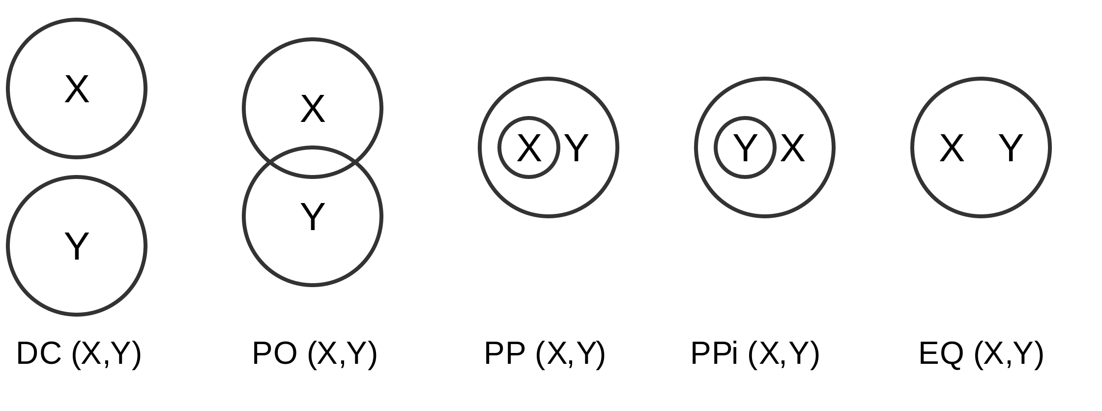
Figure 2.1: Pictorial representation of the RCC-5 relations.

Since the RCC - 5 reasoning model is used when the spatial regions are merged together, which is unlikely in our case, a three tier spatial reasoning model is proposed for further reasoning of the detected bands.

Chapter 3 Hough Lines and Low-Level Bands Generation

Most of the bands on the news video frame are made up of basic shapes like square, rectangle or in some cases, trapezium. Hence, to precisely detect these bands, detection of straight lines from the frame is one of the most important steps.
Hough transform [25] is a method used to isolate defined shapes from an image. The method works by considering the duality between points on the defined curve and its parameters. Hough transform implements a voting scheme for all potential curves in the image. Each detected edge point votes for the parameter pairs of all the curves to which it belongs. Finally, the curves that have high voting score are the ones which exists in the image. The Progressive Probabilistic Hough Transform [26] is the variation of the standard Hough transform which uses the difference in the fraction of votes to precisely detect lines. As a result, progressive probabilistic Hough transform is computationally less expensive compared to the standard Hough transform.
The progressive probabilistic Hough transform algorithm suggested by Matas et al. [26] for detecting lines can be summarized as:

1. Check the input image; if it is empty then finish.

2. Update the accumulator with a single pixel randomly selected from the input image.

3. Remove the selected pixel from input image.

4. Check if the highest peak in the accumulator that was modified by the new pixel is higher than threshold thr(N). If not, goto 1.

5. Look along a corridor specified by the peak in the accumulator, and find the longest segment that either is continuous or exhibits a gap not exceeding a given threshold.

6. Remove the pixels in the segment from input image

7. “Unvote” from the accumulator all the pixels from the line that have previously voted.

8. If the line segment is longer than the minimum length add it into the output list.

9. Goto 1.

((a)) Original Image

((b)) Detected Hough Lines

((c)) Generated Rectangular Bands

Figure 3.1: Output of Progressive Probabilistic Hough Transform

The lines detected using PPHT are then extended to image boundaries. This is done to account for the lines which could not be detected due to poor gradient.

The intersection points obtained from the extended Hough lines are then used to form the rectangular bands. These low level rectangular bands divides the entire image into different segmented profiles. In the post-processing step, the smaller profiles from the same class gets merged together to form the final image profile. The final image profile consists of non-overlapping rectangular bands, which defines the profile format which is created by merging the bands using associative reasoning.

Chapter 4 Text Detector

Raghvendra et. al. [5] proposed a two-stage contrast enhancement based pre-processing scheme for the performance improvement of gradient based text detectors, followed by the text band detection using first and second order derivatives of the gradient projection profiles.

The threshold for gradient magnitude image to generate edge map is a very important precursor for the basic text detection approaches [27][28][29]. As stated by Raghvendra [5], it is practically impossible to define a threshold which precisely separates all the text gradient values from those of non text. Due to this, generally a lower threshold is chosen to eliminate definitely non text regions followed by refinement of edge map using text specific features to obtain the text edges from edge map.
Scharr operator [30] is used to compute the normalized gradient magnitude image I_m due to its isotropic nature. The suppression of small non-zero gradient magnitude is done using the linear contrast enhancement given by:

$$I_{mc}(x,y)=\begin{cases}\dfrac{1}{\lambda}[\beta];&\beta>0\\ 0;&Otherwise\end{cases}$$ (4.1)

where $\beta$ = $\alpha($ I_mm(x,y) - 0.5) + 0.5, $\alpha$ decides the extent of enhancement and $\lambda$ is the normalization constant
The image I_mc obtained is further processed with the histogram equilization to obtain $\Omega_{ce}$, which is the contrast enhanced edge map. Horizontal Projection Profile P_hp is computed using the contrast enhanced edge map by P_hp(y) = $\sum_{x=-1}^{width}\Omega(x,y)$ . The horizontal line $y=y*$ is considered to be the member of horizontal text band H_band, if P_hp(y*) exceeds a threshold.
Vertical Projection Profile P_vp is computed within each horizontal band. For the horizontal test band H_band(y1,y2), P_vp is calculated by P_vp(x) = $\sum_{y=y1}^{y2}\Omega(x,y)$. Once again, the vertical line $x=x*$ is considered to be the member of vertical text band V_band, if P_vp(y*) exceeds a threshold.
The localization of H_band(y1,y2) and V_band(x1,x2) leads to the formation of the bounding text rectangle.

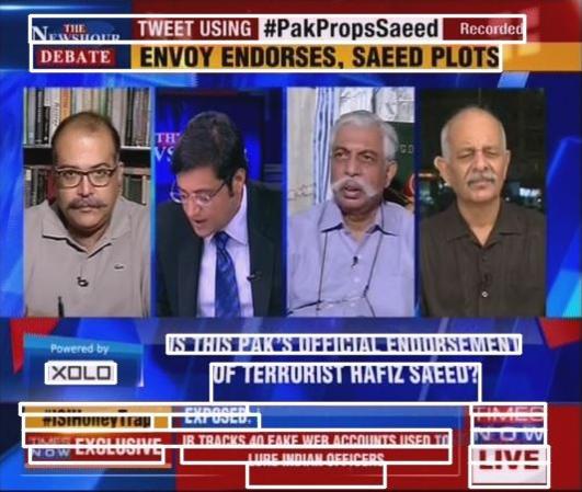
Figure 4.1: Detected text bands in different news frames

Chapter 5 The Feature Space

After the elements of a frame from a video have been extracted, it is impertive that they be classified, so as to help in a better understanding of the video format discovery. For this purpose, the images have been classified into two categories: natural images and graphics. Natural images, as the name quite clearly suggests, include images captured by cameras, such as news reporters, field shots, etc. Graphics comprise mainly of logo animations, text boxes, ticker texts and the news channel logo.

5.1 Feature Analysis for Classifier Design

This section details the features that have been used for the classification and also highlights the intuition behind each feature. The chapter has been divided into two subsections, corresponding to the color features and the spatial features.

5.1.1 Color Features

The color features are based on the color information stored in the image pixels. Although this may seem quite trivial, the color intensities of the image pixels contain a lot of information and the features extracted from them can be effectively used for the purpose of classification.

Number of different colors

In general, graphics have large areas of constant color, whereas natural photographs don’t. As a result, the number of distinct colors in a graphic image is more than that in a natural photograph. However, the number of different colors in an image is not an effective metric to consider as it depends on the size of the image. A more accurate metric is the ratio of the number of the different colors to the total number of pixels in an image. This score is generally low for graphics as compared to natural images.

$distinctColorScore=\dfrac{\text{Number of different pixels}}{\text{Total number of pixels}}$

Prevalent Color Metric

Since graphics tend to have a small number of colors and large regions of color constancy, the number of pixels having the most prevalent color is higher in graphics than natural images. Again, we cannot use the exact number of pixels for this metric, therefore, we use the ratio of the number of pixels having the most prevalent color to the total number of pixels in an image as a classification metric. This score is generally higher for graphics as compared to natural images.

$prevalentColorScore=\dfrac{\text{Number of pixels having the most prevalent color}}{\text{Total number of pixels}}$

Saturation Average

Photographs depict objects of the real world and highly saturated objects are not very common. Certain colors are much more likely to appear in graphics than in photographs. For example, animations, maps, charts and logos often have large regions covered with highly saturated colors. Those colors are much less frequent in photographs. The saturation average of graphics is expected to be greater than that of natural images.

Given RGB values, the saturation level of a pixel is defined as the greatest absolute difference of values between red, green and blue channel intensities. The saturation average is then calculted as the average of the saturation levels of all the pixels in the image.

$saturationAverage=\dfrac{\sum{max\big{(}abs(red-blue),abs(blue-green),abs(green-red)\big{)}}}{\text{Total number of pixels}}$

Saturation Metric

This metric is also based on the assumption that highly saturated colors are more common in graphics than in photographs. The saturation metric is calculated as the ratio of the number of pixels with a saturation level greater then a threshold to the total numer of pixels. The saturation metric is expected to be more for the graphics than the natural images.

$saturationScore=\dfrac{\text{Number of pixels having saturation}\geq\text{THRESHOLD}}{\text{Total number of pixels}}$

Color Histogram Metric

This metric is based on the assumption that certain colors occur more frequently in graphics than in photographs. In contrast to the saturation metric, here we do not assume anything about the nature of those colors. We simply collect statistics from a large number of graphics and photographs and construct histograms which show how often each color occurs in images of each type. The score of an image depends om the correlation of its color histogram to the graphics histogram and the photographs histogram.

A set of 500 images of each class was taken to compute the average color histogram of each class. The color histogram metric is calculated as the correlation of the image histogram with the average graphics histogram divided by the sum of the correlations of the image histogram with the average graphics histogram and the average natural image histogram.

$colorHistMetric=\dfrac{Graphics\_correlation}{Graphics\_correlation+NaturalImage\_correlation}$

Ranked Histogram

This metric is based on the same assumption as the prevalent color metric: graphics tend to have fewer colors than photographs, and the percentage of the pixels of the prevalent colors for graphics is higher. However, it is quite possible that an image can contain more than one prevalent color. In such cases, the prevalent color metric is not very efficient, and the ranked histogram feature prevails.

To begin with, each color image (which initially consists of 256 bins for each of the three R, G and B channels) is quantized into 32 bins for each channel. A 32³ (=32768) bin histogram is then created, which gives the count of each quantized color presented in the image. The histogram is normalized to unit length in L1 norm. The histogram is sorted in descending order by the value of the elements. Finally, the m largest elements are used as the ranked histogram feature.

HSV Histogram

The choice of HSV(Hue Saturation Value) color space instead of RGB can be attributed to the fact that RGB information is usually much more noisy than the HSV information. This is because unlike RGB, HSV separates luma, or the image intensity, from chroma, or the color information.

Previous work done by Yuanhao Chen et al. [16] used the moments (mean, standard deviation and skewness) of the histogram data from each of the three channels (H, S and V). However, it is not possible to encompass all the data using only these three moments. Therefore, it is proposed to use the entire 768 bin (256 bins per channel * 3 channels) histogram as a feature for classification purpose.

5.1.2 Spatial Features

The color analysis gives some pretty good features that can be used for the classification of images. However, it does not take in account the spatial correlation of pixels. For example, graphics tend to have sharp color gradients, which is not quite the case with natural images. Also, because of the way the natural images are acquired, they tend to have some inherent noise, which is hardly present in graphics.
Different spatial features have been implemented and discussed below.

Farthest Neighbor Metric

This metric is based on the assumption about how color transitions are different in graphics and natural images. Graphics have comparatively sharp color transitions and large regions of constant colors as compared to natural images, which have smoother color transitions.

For any pixel $p_{1}$ and its neighbor $p_{2}$ with their color vectors in the RGB color space given as $(r,g,b)$ and $(r^{\prime},g^{\prime},b^{\prime})$ respectively, their color distance d is defined as:

$d=\big{(}abs(r-r^{\prime})+abs(g-g^{\prime})+abs(b-b^{\prime})\big{)}$

Since the pixel intensity values go from 0 to 255, the value of d can go from 0 to 765. A threshold between 0 and 765 is specified, and the farthest neighbor score of an image is the fraction of pixels having a color distance d greater than or equal to the threshold. This score is generally higher for graphics as compared to natural images.

$farthestNeighbourScore=\dfrac{\text{Number of pixels for which {d}}\geq\text{THRESHOLD}}{\text{Total number of pixels}}$

Farthest Neighbor Histogram Metric

This metric is based on similar assumptions as the farthest neighbor metric. However, this is a different metric as it utilizes the correlation between the farthest neighbor histogram of the test image with the average farthest neighbor histograms of the graphics and the natural images.

The farthest neighbor histogram of an image is a one-dimensional histogram with 766 bins. The i^th bin contains the fraction of pixels with transition value equal to i. The possible of transition values are 0 + 255*3 (for each of the three channels) = 766 total transition values.

Using the same dataset of 500 images for each class that was used to generate the average color histogram for the computation of the color histogram metric, we find the average farthest neighbor histogram for each class, and denote them by $FNH_{natural}$ (for natural images) and $FNH_{graphics}$ (for graphics). We define the correlation between two histograms X and Y as

$$C(X,Y)=\displaystyle\sum_{i=0}^{765}X_{i}Y_{i}\\$$

where $X_{i}$ and $Y_{i}$ are the i^th bins of X and Y respectively.
Let $FNH_{image}$ be the farthest neighbor histogram of a test image. The farthest neighbor histogram score of the image is calculated as

$farthestNeighbourHistMetricScore=\dfrac{nat}{nat+graph}$

where $nat=C(FNH_{image},FNH_{natural})$ and $graph=C(FNH_{image},FNH_{graphics})$. Similar to the farthest neighbor metric, the farthest neighbor histogram metric is expected to be higher for the natural images than for the graphics.

Gray Histogram Smoothness

As mentioned in the earlier subsubsections, graphics generally tend to have sharper color transitions than natural images. This is also reflected in the gray histogram data. The graphics histogram shows some narrow and sharp peaks because of the selective use of some dominant colors, while this trend is not quite visible on a natural image histogram.

The gray histogram smoothness of an image is calculated as: The gray level histogram of the image is first calculated. The histogram is then normalized by dividing the value of all bins by the number of pixels. The smoothness is the absolute sum of the bin value transitions for all bins in the gray histogram.

$$smoothness=\displaystyle\sum_{i=1}^{255}\big{(}grayHist[i]-grayHist[i-1]\big{)}\\$$

Edge Magnitude Histogram

The underlying principle as to why this feature has been incorporated in the classifier is that the graphics tend to have strong (prominent) edges, and they are less in number. On the other hand, the natural images generally have weaker edges, and they are comparatively more in number.

For a given image, its edge magnitude histogram is calculated, and the result is stored in 32 bins. This 32-bin histogram is then used as a feature for the classifier.

Chapter 6 Classification Scheme

6.1 Support Vector Machine

A Support Vector Machine (SVM) with a radial basis function (RBF) kernel has been chosen as the classifier, and the SVM parameter estimation was optimised using grid-search with 10-fold cross validation [18].

6.2 Extreme Learning Machine

While using feedforward ANNs (Artificial Neural Networks), all the parameters need to be tuned and thus a dependency exists between the parameters (the weights and the biases) of the different layers. Gradient descent based learning methods have been used for learning these parameters, but they are very slow and may give inaccurate results because of convergence to local minima.

Proposed by Guang-Bing Huang et al. in 2006, extreme learning machine (ELM) [31][32][33] is a learning algorithm for SLFNs (Single Layer Feedforward Networks) having order of magnitudes times faster learning speed and better generalization performance than the classical feedforward network learning algorithms like the Back Propagation Algorithm.

6.2.1 Theory

For a generalized SLFN, the hidden layer mapping can be described as:

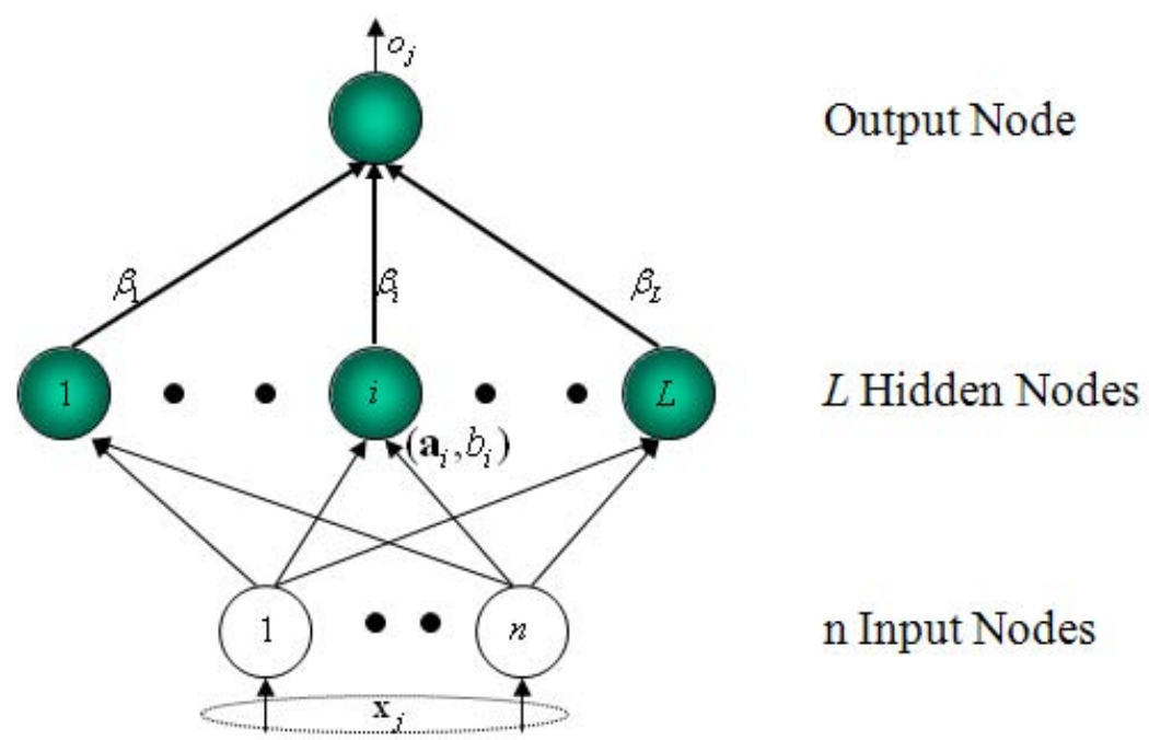
Figure 6.1: Generalized Single Layer Feedforward Network

• Output function of SLFNs:
  $f_{L}(\textbf{x})=\sum_{i=1}^{L}\beta_{i}G(\textbf{a}_{i},b_{i},\textbf{x})$

• The hidden layer output function:
  $h(\textbf{x})=[G(\textbf{a}_{1},b_{1},\textbf{x}),\ldots,G(\textbf{a}_{L},b_{L},\textbf{x})]$

• The output functions of the hidden nodes can be but are not limited to:
  Sigmoid: $G(\textbf{a}_{i},b_{i},\textbf{x})=g(\textbf{a}_{i}\cdot\textbf{x}+b_{i})$
  Radial Basis Function: $G(\textbf{a}_{i},b_{i},\textbf{x})=g(b_{i}\left\|\textbf{x}-\textbf{a}_{i}\right\|)$

where,
$\beta_{i}$ is the weight vector connecting the $i^{th}$ hidden node and the output nodes, $i=1,\ldots,L$
$\textbf{a}_{i}$ is the weight vector connecting the input nodes and the $i^{th}$ hidden node, $i=1,\ldots,L$
$b_{i}$ is the bias vector connecting the $i^{th}$ hidden node and the input nodes, $i=1,\ldots,L$

Given: Training set $\aleph=\{(\textbf{x}_{i},\textbf{t}_{i})|\textbf{x}_{i}\in\mathbf{R}^{n},\textbf{t}_{i}\in\mathbf{R}^{m},i=1,\ldots,N\}$, hidden node output function $G(\textbf{a},b,\textbf{x})$, mumber of hidden nodes $L$ 

Assign: Randomly generated values to the hidden node parameters $(\textbf{a}_{i},b_{i}),i=1,\ldots,L$. 

Calculate: The hidden layer output matrix H, the $i^{th}$ column of which is the output of the $i^{th}$ hidden node with respect to the inputs $\textbf{x}_{i},\ldots,\textbf{x}_{N}$. 

Calculate: The output weight matrix $\beta$ is calculated as $\beta=\textbf{H}^{\dagger}\textbf{T}$, where $\textbf{H}^{\dagger}$ is the pseudoinverse of H, and $\textbf{T}=[\textbf{t}_{1}^{T},\ldots,\textbf{t}_{N}^{T}]^{T}$, $\textbf{t}_{j}=\sum_{i=1}^{L}\beta_{i}G(\textbf{a}_{i},b_{i},\textbf{x})$. 

Algorithm 1 Extreme Learning Machine Training

The salient features and advantages of ELMs are as listed below:

• The learning speed of ELM is extremely fast.

• The hidden node parameters $\textbf{a}_{i}$s and $b_{i}$s are independent of the data and also of each other.

• ELM does not encounter traditional gradient-based learning issues, such as, local minima, improper learning rate, overfitting etc.

Chapter 7 Band Identification Through Change Detection

One of the main factors that distinguish artificial bands from the natural bands is that the content of the artificial bands tends to be static over certain range of frames. This is because of the fact that natural bands contain images captures from cameras, such as news reporters, field shots etc., which is updated in each frame while the artificial bands contain computer generated graphics like logo animations, text boxes and ticker texts which remain static over a certain range of frames. This information is used to differentiate between the two bands. Two types of change detection methods were used.

1. Pixels based change detection.

2. Histogram based change detection.

7.1 Pixels Based Change Detection

For pixels based change detection, a difference image is created for each frame which is the pixel-wise difference between the current frame grey image and the previous frame grey image.

$$d^{k}(x,y)=I^{k}(x,y)-I^{k-1}(x,y)$$ (7.1)

where, $d_{k}$ is the difference image for the $k$th frame while $I^{k}$ and $I^{k-1}$ are the $k$th and $k-1$th frame respectively. Next, the difference image is binarized using a threshold. If the absolute value of difference pixel is greater than the threshold, it is labeled as $1$, otherwise $0$. This binarized image is further divided into $N$x$N$ sub-images and the sub-image is labeled according to the majority of the pixels in that sub-image. The natural sub-image is the one with its label as $1$, and the artificial sub-image is one with its label as $0$.

7.2 Histogram Based Change Detection

For histogram based change detection, first of all, the image is converted into a monochrome image according to the equation 8.1. For the change detection on the $k^{th}$ frame, the $k^{th}$ and the $(k-1)^{th}$ frame are each divided into $N$x$N$ sub-images. Then the histogram is calculated for these sub-images. Corresponding to each sub-image, Bhattacharya distance (Equation 8.2) is calculated between the histogram of current frame’s sub-image and the histogram of the previous frame’s sub-image. If the distance is greater than a given threshold then the sub-image is labeled as natural image, otherwise it is labeled as artificial.

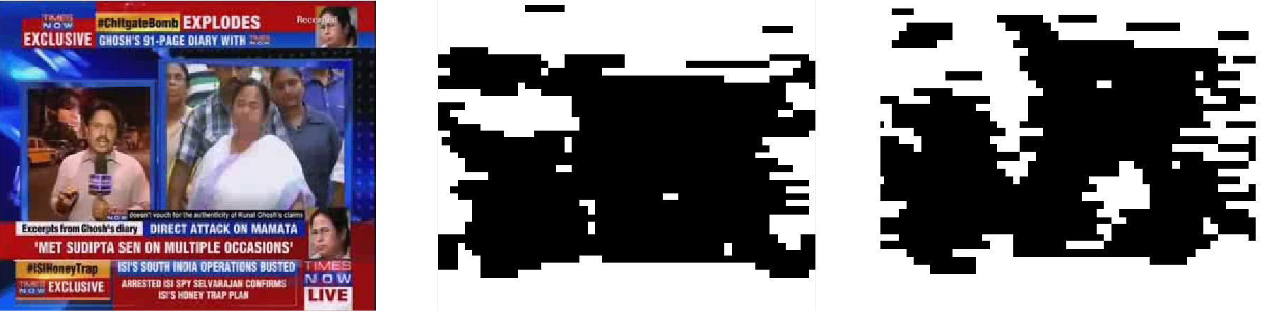
Figure 7.1: Output of the change detection (a) Rectanglular bands detected from Hough Lines, (b) Output of the pixels based change detection with N = 50, (c) Output of the histogram based change detection with N = 50.

In addition to the classifier output, the change based band identification is used to improve the accuracy and provide better result after associative reasoning.

Chapter 8 Associative Reasoning

The low level rectangular bands after the Hough transformation are obtained by using Hough lines extended till the image boundaries. These bands can be broadly categorized into three categories:

1. Synthetic Bands: Synthetic bands are the bands generated artificially using computer graphics. They usually includes logo animations, text boxes, ticker texts and the news channel logo.

2. Natural Bands: Natural bands, as the name quite clearly suggests, include bands captured by cameras, such as news reporters, field shots, etc.

3. Text Bands: Text bands are the bands containing texts.

Because of the Hough lines extended till the image boundaries, the entire text band gets split into various smaller bands. To compensate for this, the small rectangular bands need to be merged together using associative reasoning. The entire reasoning model can be hierarchically divided into three sub-reasoning models. They are,

1. Merging of the bands with similar histograms, used for the merging of synthetic bands.

2. Merging of the bands labeled as natural bands using the SVM classifier.

3. Merging of the bands labeled as text bands using the text detector.

For the fast and easy implementation of the associative reasoning, an adjacency matrix is created for each frame. An adjacency matrix $A$, is a $NXN$ square matrix, where $N$ is the total number of bands detected from the frame.

$a_{ij}$ = $\alpha$ where $\alpha$ $\in$ $\{$ $0,1,2,3,4$ $\}$. Here, $a_{ij}$ is the element of $i$th row of A and $j$th column of A.

$a_{ij}$ = $1$ ,if the $j$th band share a boundary with the $i$th band and is above the $i$th band.

$a_{ij}$ = $2$ ,if the $j$th band share a boundary with the $i$th band and is to the right of the $i$th band.

$a_{ij}$ = $3$ ,if the $j$th band share a boundary with the $i$th band and is below the $i$th band.

$a_{ij}$ = $4$ ,if the $j$th band share a boundary with the $i$th band and is to the left of the $i$th band.

$a_{ij}$ = $0$ ,if $a_{ij}$ $\notin$ $\{$ $1,2,3,4$ $\}$ , that is, the $i$th and the $j$th band does not share a boundary with each other.

8.1 Merging Rules

If two text bands $\textit{H${}_{band_{i}}$}(x_{i},y_{i},h_{i},w_{i})$ with its left corner at $(x_{i},y_{i})$, width $w_{i}$ and height $h_{i}$; and $\textit{H${}_{band_{j}}$}(x_{j},y_{j},h_{j},w_{j})$ are merged together to form $\textit{H${}_{band_{k}}$}(x_{k},y_{k},h_{k},w_{k})$. And if,

1. $a_{ij}$ = $1$, then

   $$x_{k} =x_{j} y_{k} =y_{j}$$

   $$h_{k} =h_{i}+h_{j} w_{k} =w_{j}$$

2. $a_{ij}$ = $2$, then

   $$x_{k} =x_{i} y_{k} =y_{i}$$

   $$h_{k} =h_{i} w_{k} =w_{i}+w_{j}$$

3. $a_{ij}$ = $3$, then

   $$x_{k} =x_{i} y_{k} =y_{i}$$

   $$h_{k} =h_{i}+h_{j} w_{k} =w_{i}$$

4. $a_{ij}$ = $4$, then

   $$x_{k} =x_{j} y_{k} =y_{j}$$

   $$h_{k} =h_{j} w_{k} =w_{i}+w_{j}$$

8.2 Merging of the bands with similar histograms

In the first step of associative reasoning, the synthetic bands need to be merged together. This is done by comparing the histograms of two bands. As the synthetic band is uniformally colored or generally does not have much color gradient, its sub-divided bands can be identified using a histogram comparison approach. Adjacent bands having similar histograms are the sub-bands of the same parent synthetic band and hence are merged together.

For computing the histogram, firstly, the RGB band image is linearly mapped to have pixel values from $0$ to $32$. Then this RGB image is converted to a monochrome image using the function

$$I_{mc}(x,y)=32^{2}*I_{r}(x,y)+32*I_{g}(x,y)+I_{b}(x,y)$$ (8.1)

where, $I_{mc}$ is the monochrome image and $I_{r}$, $I_{g}$ and $I_{b}$ are the red, green and blue channels of the RGB image respectively.

Next, normalized histograms are calculated for both the monochrome images. The similarity between both the histograms is measured using the Bhattacharya distance. The Bhattacharya distance between two histograms $H_{1}$ and $H_{2}$ can be calculated as

$$d(H_{1},H_{2})=\sqrt{1-\dfrac{1}{\sqrt{\bar{H_{1}}\bar{H_{2}}N^{2}}}\sum_{I}\sqrt{H_{1}(I).H_{2}(I)}}$$ (8.2)

where,

$$\bar{H_{k}}=\dfrac{1}{N}\sum_{J}H_{k}(J)$$ (8.3)

Similar histograms have a Bhattacharya distance close to $0$, while two dissimilar histograms have a Bhattacharya distance closer to $1$. Hence, if the two bands share a boundary and have a Bhattacharya distance less than a threshold, then they are merged together according to the merging rules mentioned above.

8.3 Merging of the natural bands

A SVM classifier, which is described in Chapter 6 is used to classify the bands into artificial and natural bands. As mentioned before, natural bands are the bands captured by cameras, such as news reporters, field shots, etc and hence sub-divided natural bands needs to be merged to form a complete natural shot frame. Two bands labeled as natural are merged together only if they both share a common boundary but there is no edge present along that common boundary. The bands are merged together according to the merging rules mentioned above.

8.4 Merging of the Text bands

The text detector mentioned in Chapter 4 is used to detect the regions of text in the frame. A low level rectangular band is labeled as text band using the overlap criterion

$$J(R,T)=\dfrac{A(R\cap T)}{A(R)}$$ (8.4)

where, $J(R,T)$ is the text overlap measure of the rectangular band $R$ and text region $T$, $A(R\cap T)$ is the area of intersection of band $R$ and text region $T$, while $A(R)$ is the area of band $R$.

Two bands with the text overlap measure greater than a given threshold are merged together only if they both share a common boundary and are horizontally adjacent to each other. The bands are merged together according to the merging rules mentioned above.

((a))

((b))

Figure 8.1: Output after merging of the bands containig text (a) Rectanglular bands detected from Hough Lines, (b) Output after the application of associative reasoning.

Chapter 9 Results

9.1 Element Band Detection

The format detection approach was tested on 100 images generated from various news channels and different shows to measure its robustness on different types of format profile.
Jaccard Index [34] is used as a measure of similarity between the obtained result and the ground truth. For two rectangular bands $R_{1}$ and $R_{2}$, Jaccard Index J($R_{1},R_{2}$) is defined as

$$J(R_{1},R_{2})=\dfrac{A(R_{1}\cap R_{2})}{A(R_{1}\cup R_{2})}\\$$

where, $A(R_{1}\cap R_{2})$ is the area of intersection of $R_{1}$ and $R_{2}$ and $A(R_{1}\cup R_{2})$ is the area of union of $R_{1}$ and $R_{2}$. A Jaccard Index of 1 signifies 100% overlap of the two bands. For the entire image frame $\textit{I}_{frame}$, the net Jaccard Index is calculated as

$$J(\textit{I}_{res},\textit{I}_{gt})=\dfrac{\sum_{i=1}^{n_{1}}\max_{1\leq j\leq n_{2}}(J(R_{i},R_{j}))}{n_{2}}\\$$

where, $\textit{I}_{res}$ is the output of the format detector containing bands $R_{i}$ for $i=1,2,3....n_{1}$ and $\textit{I}_{gt}$ is the ground truth containing bands $R_{j}$ for $j=1,2,3....n_{2}$
The average Jaccard Index of the entire dataset of 100 images was calculated to be $0.8138$.

9.2 Element Band Classification

The Support Vector Machine (SVM) with a Radial Basis Function (RBF) kernel was trained using LibSVM tool over a dataset of 6000 images, with equal number of images from both the classes. A total of eleven features (color features and spatial features) were used for classifier training. The feature vectors were 1320-dimensional each. The entire process of feature extraction, SVM training and performance analysis (10-fold cross validation and testing) took 530 minutes on an average on an Intel Core i7 Ivy Bridge machine running 64-bit Ubuntu OS with 8 GB of RAM, when utilizing all the 8 cores in parallel using GNU Parallel [35].

The Extreme Learning Machine (ELM) was also trained on the same dataset of 6000 images, each feature vector being 1320-dimensional. The training and performance analysis was comparatively faster than that of SVM.

9.3 Performance Measures

9.3.1 Precision

Precision is a measure of the accuracy provided that a specific class has been predicted. It is defined as:

Precision = $\dfrac{\text{TP}}{\text{TP + FP}}$

where TP and FP are the numbers of true positive and false positive predictions for the considered class.

9.3.2 Recall

Recall is a measure of the ability of a prediction model to select instances of a certain class from a data set. Since we are dealing with binary classification here, the recall is also called as sensitivity. The recall (or sensitivity) corresponds to the true positive rate, and is defined as:

Recall = Sensitivity = $\dfrac{\text{TP}}{\text{TP + FN}}$

where TP and FN are the numbers of true positive and false negative predictions for the considered class. Thus, (TP + FN) corresponds to the total number of test examples of the considered class.

9.3.3 F-measure

The F-measure (also known as $F_{1}$-score), is a more accurate metric of classifier performance than either precision or recall alone. In binary classification, the F-measure is the harmonic mean of the precision and the recall, as is calculated as:

F-measure = 2 $\dfrac{\text{Precision . Recall}}{\text{Precision + Recall}}$

9.3.4 Balanced Accuracy

Evaluating the performance of a classification by averaging the accuracies obtained on individual cross-validation folds is not a very good approach [36] due to two main reasons. Firstly, it does not allow for the derivation of meaningful confidence intervals. Secondly, it leads to an optimistic estimate when a biased classifier is tested on an imbalanced dataset. Balanced accuracy, which is defined as the arithmetic mean of the sensitivity and the specificity of the classifier, does away with inflated performance estimates on imbalanced datasets.

Balanced Accuracy = $\dfrac{\text{Sensitivity + Specificity}}{2}$ = $\dfrac{\text{0.5*TP}}{\text{TP + FN}}+\dfrac{\text{0.5*TN}}{\text{TN + FP}}$

where TP, TN, FP and FN are the numbers of true positive, true negative, false positive and false negative predictions.

9.4 Performance Analysis

9.4.1 SVM Performance Analysis

A graphical representation of the classifier performance for each of the 11 features has been attached in the next page. A more detailed analysis follows.

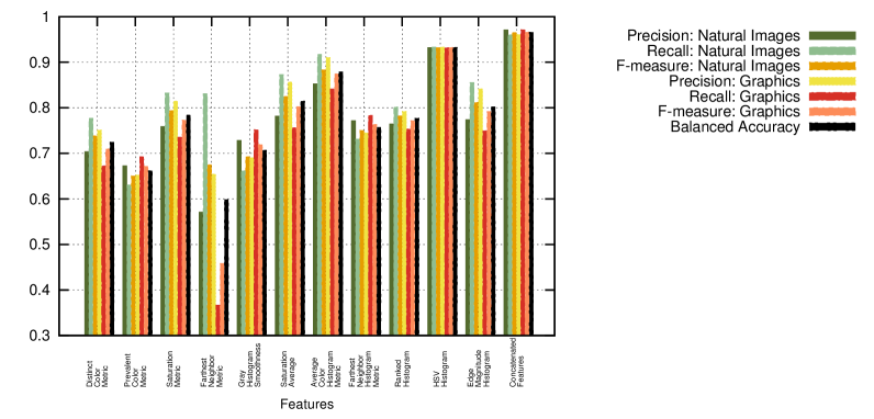
Figure 9.1: Performance analysis of the designed SVM classifier on individual features and their combination. The comparison of precisions, recalls and f-measures for both natural images and graphics categories are shown. Note that the HSV Histogram dominates as a feature.

10-fold cross-validation and testing was performed on the dataset to analyse the performance of individual features as well as the concatenated features. The results have been plotted for all of them and are as shown below:

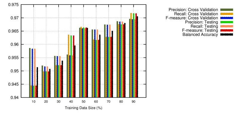
Figure 9.2: Performance analysis of concatenated features with varying data size

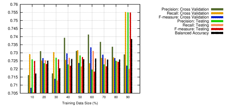
Figure 9.3: Performance analysis of Distinct Color Metric with varying data size

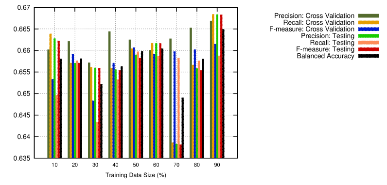
Figure 9.4: Performance analysis of Prevalent Color Metric with varying data size

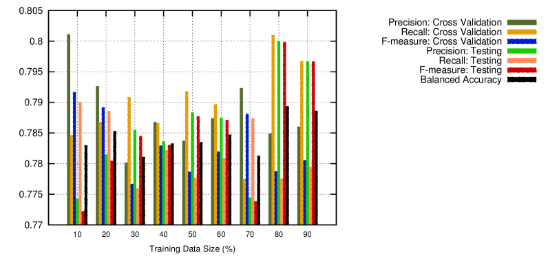
Figure 9.5: Performance analysis of Saturation Metric with varying data size

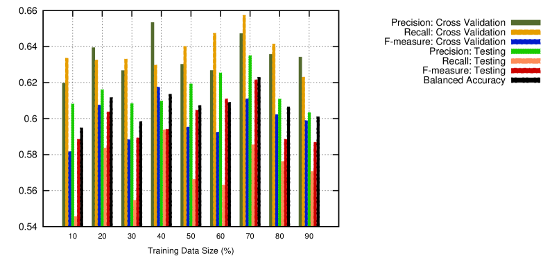
Figure 9.6: Performance analysis of Farthest Neighbor Metric with varying data size

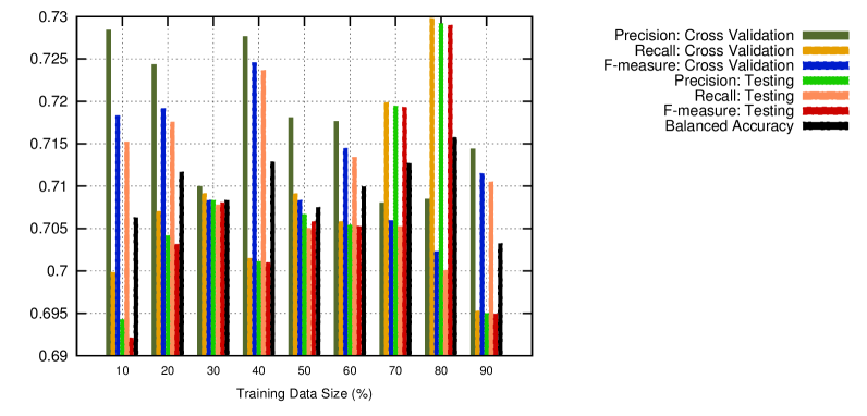
Figure 9.7: Performance analysis of Gray Histogram Smoothness with varying data size

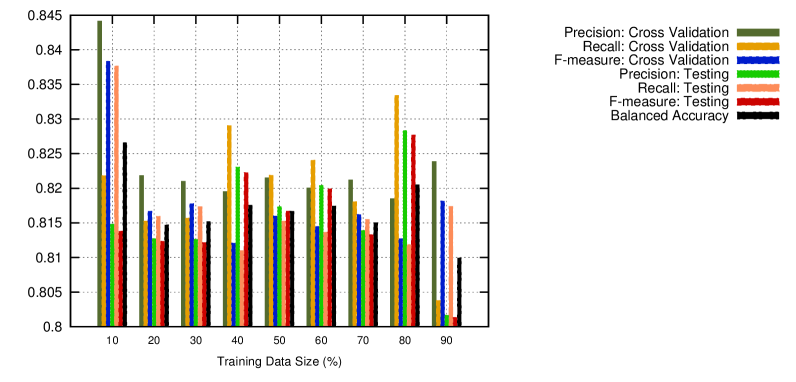
Figure 9.8: Performance analysis of Saturation Average with varying data size

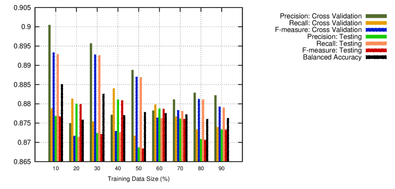
Figure 9.9: Performance analysis of Average Color Histogram Metric with varying data size

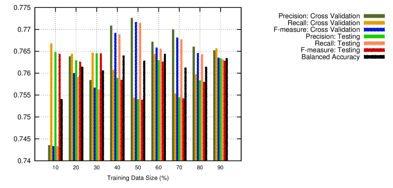
Figure 9.10: Performance analysis of Farthest Neighbor Histogram Metric with varying data size

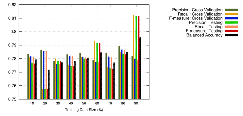
Figure 9.11: Performance analysis of Ranked Histogram with varying data size

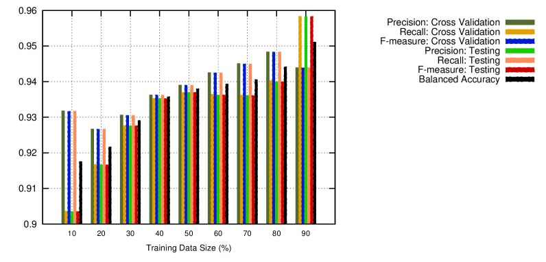
Figure 9.12: Performance analysis of HSV Histogram with varying data size

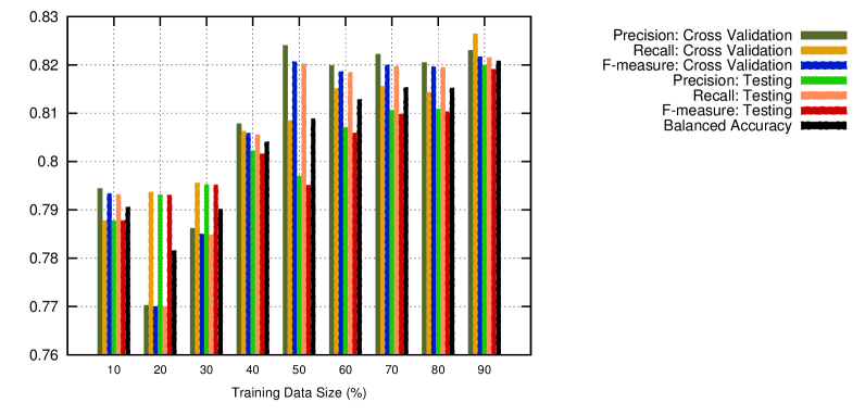
Figure 9.13: Performance analysis of concatenated features with varying data size

The concatenated features have a balanced accuracy of 96.57%. The HSV histogram and the farthest neighbor metric fared the best and worst in individual performance with balanced accuracies of 93.23% and 59.86% respectively.

9.4.2 ELM Performance Analysis

As mentioned previously, the ELM was trained on 3000 feature vectors of each class, 1320-dimensional each. The input weight matrix and the bias matrix were composed of values chosen randomly between -3 and 3. The following figure plots the F-measure for both the classes and the overall balanced accuracy of the ELM classifier.

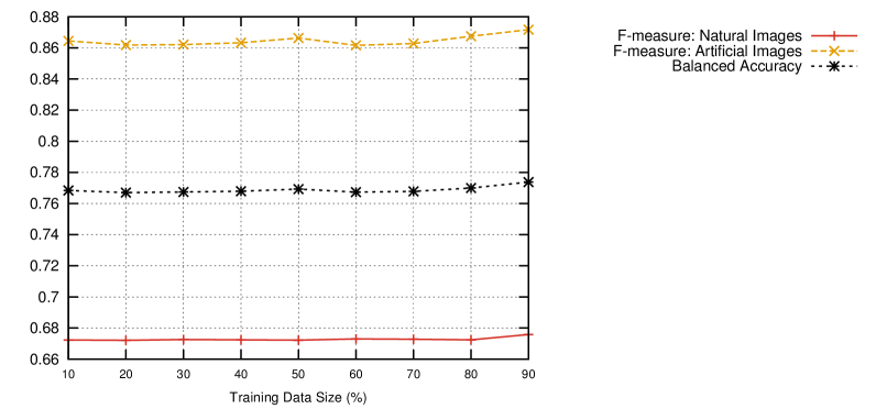
Figure 9.14: Performance analysis of the designed ELM classifier trained on varying dataset of varying size. The variation of F-measure of both the classes and the balanced accuracy according to the training dataset size is plotted.

From the figure, it is clear that the ELM classifier is inferior to the SVM classifier for our application. Therefore, no detailed performance analysis was done for the ELM classifier and the SVM classifer was used for classification of the extracted bands.

Chapter 10 Conclusion

In our project, we have successfully come up with a robust approach to detect the format of broadcast news videos. Unlike previous work done in this field, our approach assumes no prior information about the news video format. This ensures that our approach works efficiently for unknown news formats as well.

A $1320$-dimensional feature vector is proposed which is used to classify the natural and the artificial bands. A text detector is used to detect the text regions. Finally, all the bands are merged together using a three-tier hierarchical reasoning to form the final format profile.

The entire broadcast format is represented in the form of rectangular bands containing either text, natural shots or computer generated graphics. As the entire news information is represented only through the text bands and natural shots, by removing the redundant information from computer generated graphics and converting the text images to machine encoded text, a significant reduction in the storage space can be achieved.

Chapter 11 Future Work

Our current approach accurately detects the profile bands from the video frames. This approach can be extended so as to track the moving bands in the video with an aim to detect the band animation format. This could play a very important role in detecting news shows and also in other news video analysis tasks. Further work in this could be to detect non-rectangular and overlapping bands as well. This work, when applied to a news video in conjunction with the output of the semantic story segmentation and video shot linking, could be used as an effective way to generate the entire news summary. As of now we are dealing with video data recorded from 4 English news channels namely, CNN IBN, Times Now, NDTV 24x7 and BBC WORLD. To measure the robustness of the final proposed approach, it could also be tested on vernacular as well as other international news channels.

11.1 Improving the Classification Accuracy

The present classifier has classification accuracy of around $95\%$ (precision, recall, F-measure and balanced accuracy) for both the classes. However, there are a few more features that can be incorporated to further improve the classifier performance.

11.1.1 Color Correlogram

A color correlogram is an effective description of the global distribution of the local spatial correlation of colors. As mentioned before, because of the way natural images are acquired using a camera, they tend to have some inherent noise, therefore making them more noisy than graphics. This property can be exploited using a color correlogram.

A color correlogram of an image is a two-dimensional matrix where. Each entry (x, y) in the matrix stores the probabilty that the given pixel (x, y) has the same color (or within a certain threshold) as its neighbors. This kind of feature is not possible to obtain using a simple color histogram since it only gives only information about the color distribution in an image, but no information about spatial correlation of the colors.

11.1.2 Spatial Gray Level Dependence

A Spatial Gray Level Dependence (SGLD henceforth) Histogram (also known as Co-occurence Matrix) is an effective representation of the image texture and in particular, the image sharpness. A SGLD histogram is a two-dimensional histogram. It denotes the joint probabilty of the occurence of two gray levels ‘i’ and ‘j’ with a defined spatial relation in terms of distance ‘d’ and angle ‘$\theta$’. For each image, a gray level transformation is obtained, and it obtained by averaging the intensity values of the three R, G and B channels.

$$brightness=\dfrac{red+green+blue}{3}\\$$

For each pixel in the image, if the pair (the pixel under consideration) and its neighbor belong to an area of color constancy (i.e. having the same brightness), an entry on the SGLD matrix diagonal is incremented by one. However, if the pair being considered lies on an edge (i.e. the two pixels belong to two different regions), the brightness levels might be similar, but not the same (in case of a weak edge) or they can be quite significantly different (in case of a strong/sharp edge). In the latter case, an entry far from the diagnonal of the SGLD matrix is incremented, while in the former case, an entry not so far from the diagnonal is incremented.

11.1.3 Local Binary Patterns

Ever since their first use in 1994, Local Binary Patterns (LBPs henceforth) have remained a efficient feature for texture description and classification. Since there is a good amount of textural information that can be levaraged in the binary classification being dealt with here, LBPs can prove to be a powerful feature.

The LBP feature vector for an image is created by comparing the pixel intensity values of all the neighbors of a particular pixel. A value of ‘0’ is assigned to the neighbor if it has an intensity greater than that of the centre pixel, else a value of ‘1’ is assigned. The assigned values are then read clockwise starting from the top left, and the binary number thus obtained is converted to decimal representation. This number is then assigned to the centre pixel. This process is repeated for the entire image, and has been illustrated below:

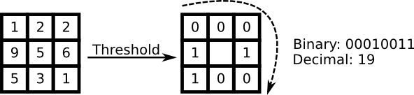
Figure 11.1: LBP computation considering an 8-neighborhood

The algorithm for the same has been detailed below:

11.2 Better algorithm for labeling the bands

One of the shortcomings encountered while labeling the extracted bands is that because of the bands breaking up into multiple fragments, one or more of the natural band fragments tend to be labeled as artificial. This poses a problem because since adjacent bands are assigned different labels, it is not possible to merge them. Note that the converse of this is not true, i.e. no artificial bands are ever classified as natural.

((a)) Original Image

((b)) Most of the face in one image

((c)) Partial face image, which gets labeled as artificial

Figure 11.2: Single band split into multiple fragments because of the extension of Hough lines.

A better labelling algorithm that can be tried in the future is as described below:
Step 1: Extract all the fragmented bands from a frame.
Step 2: Compute the HSV histogram of all the fragmented bands, and perform incremental clustering using the HSV histogram data as the feature vectors. This clustering of the fragmented bands based on their similarity ensures that fragments which are part of the same band get assigned to the same cluster.
Step 3: Assign labels to the bands using the classifier as usual.
Step 4: For each cluster, if any band in the cluster has been classified as natural, assign the natural label to all the bands in the cluster.

Chapter 12 Appendix

12.1 Ground Truth Marking Tool

As the data used for training and testing of our approach is self-generated from various recorded news channels, a ground truth marking tool is developed in OpenCV, to efficiently generate the ground truth results of all the dataset images.

The tool loads an image and displays it on the screen. The user has to mark rectangular regions of interest with the mouse by selecting top left and bottom right corner of the rectangular bands. A text file is created for each image and after marking all the bands (both artificial and natural), the bands’ positions are dumped in the respective text file. For calculating the accuracy, the result is compared with the ground truth, which is obtained by reading the text file of the respective testing image.

12.2 Dataset Generating Tool

The classifier has been trained on 3000 images of artificial and natural categories each. Since the images to be classified are the components of the news frames, the training data is also generated from the news frames. In order to achieve this, a simple tool is developed.

Given an image, the Hough rectangles are detected in the image as mentioned earlier. Then, a window is shown with the image and the Hough rectangles are shown on the image one by one starting from the bottom left of the image. The user provides input from the keyboard, indicating whether the rectangle currently being shown belongs to the artificial category or the natural category. We have assigned two keys, one for each class. Upon the user input, the rectangle gets dumped into the corresponding folder.

After the dataset has been generated, the feature vectors are generated for the images and are then used for classifier training.

Bibliography

- [1] S. Eickeler and S. Muller. Content-based video indexing of tv broadcast news using hidden markov models. In Acoustics, Speech, and Signal Processing, 1999. Proceedings., 1999 IEEE International Conference on, volume 6, pages 2997–3000 vol.6, Mar 1999.
- [2] Lie Lu and Hong-Jiang Zhang. Speaker change detection and tracking in real-time news broadcasting analysis. In Proceedings of the Tenth ACM International Conference on Multimedia, MULTIMEDIA ’02, pages 602–610, New York, NY, USA, 2002. ACM.
- [3] David Hillman. Multimedia technology and applications. In Golgotia Publications Pvt. Ltd., page 9.
- [4] K. K. Thyagharajan and V. Ramachandran. Performance analysis of media transmission through low bandwidth networks. In National Conference on Signal Processing, Intelligent Systems and Networking, 2003.
- [5] Raghvendra Kannao and Prithwijit Guha. A novel preprocessing scheme for text detection in broadcast news videos (under review).
- [6] Andrew Merlino, Daryl Morey, and Mark Maybury. Broadcast news navigation using story segmentation. In Proceedings of the Fifth ACM International Conference on Multimedia, MULTIMEDIA ’97, pages 381–391, New York, NY, USA, 1997. ACM.
- [7] Dong Xu and Shih-Fu Chang. Visual event recognition in news video using kernel methods with multi-level temporal alignment. In Computer Vision and Pattern Recognition, 2007. CVPR ’07. IEEE Conference on, pages 1–8, June 2007.
- [8] Hangzai Luo, Jianping Fan, Jing Yang, W. Ribarsky, and S. Satoh. Analyzing large-scale news video databases to support knowledge visualization and intuitive retrieval. In Visual Analytics Science and Technology, 2007. VAST 2007. IEEE Symposium on, pages 107–114, Oct 2007.
- [9] Hangzai Luo, Jianping Fan, Jing Yang, W. Ribarsky, and S. Satoh. Exploring large-scale video news via interactive visualization. In Visual Analytics Science And Technology, 2006 IEEE Symposium On, pages 75–82, Oct 2006.
- [10] Hongjiang Zhang, Yihong Gong, S.W. Smoliar, and Shuang Yeo Tan. Automatic parsing of news video. In Multimedia Computing and Systems, 1994., Proceedings of the International Conference on, pages 45–54, May 1994.
- [11] Vassilis Athitsos, Michael J Swain, and Charles Frankel. Distinguishing photographs and graphics on the world wide web. In Content-Based Access of Image and Video Libraries, 1997. Proceedings. IEEE Workshop on, pages 10–17. IEEE, 1997.
- [12] Charles Frankel, Michael J Swain, and Vassilis Athitsos. Webseer: An image search engine for the world wide web. 1996.
- [13] J. Ross Quinlan. Induction of decision trees. Machine learning, 1(1):81–106, 1986.
- [14] Jing Huang, S Ravi Kumar, Mandar Mitra, Wei-Jing Zhu, and Ramin Zabih. Image indexing using color correlograms. In Computer Vision and Pattern Recognition, 1997. Proceedings., 1997 IEEE Computer Society Conference on, pages 762–768. IEEE, 1997.
- [15] Rainer Lienhart and Alexander Hartmann. Classifying images on the web automatically. Journal of Electronic Imaging, 11(4):445–454, 2002.
- [16] Yuanhao Chen, Zhiwei Li, Mingjing Li, and Wei-Ying Ma. Automatic classification of photographs and graphics, February 2 2010. US Patent 7,657,089.
- [17] Markus A Stricker and Markus Orengo. Similarity of color images. In IS&T/SPIE’s Symposium on Electronic Imaging: Science & Technology, pages 381–392. International Society for Optics and Photonics, 1995.
- [18] Yoshua Bengio and Yves Grandvalet. No unbiased estimator of the variance of k-fold cross-validation. The Journal of Machine Learning Research, 5:1089–1105, 2004.
- [19] Tian-Tsong Ng, Shih-Fu Chang, Jessie Hsu, Lexing Xie, and Mao-Pei Tsui. Physics-motivated features for distinguishing photographic images and computer graphics. In Proceedings of the 13th annual ACM international conference on Multimedia, pages 239–248. ACM, 2005.
- [20] Fei Wang and Min-Yen Kan. Npic: Hierarchical synthetic image classification using image search and generic features. In Image and Video Retrieval, pages 473–482. Springer, 2006.
- [21] Yossi Rubner, Carlo Tomasi, and Leonidas J Guibas. The earth mover’s distance as a metric for image retrieval. International Journal of Computer Vision, 40(2):99–121, 2000.
- [22] Robert E Schapire and Yoram Singer. Boostexter: A boosting-based system for text categorization. Machine learning, 39(2-3):135–168, 2000.
- [23] A.G. Cohn. Qualitative spatial representation and reasoning techniques. In Gerhard Brewka, Christopher Habel, and Bernhard Nebel, editors, KI-97: Advances in Artificial Intelligence, volume 1303 of Lecture Notes in Computer Science, pages 1–30. Springer Berlin Heidelberg, 1997.
- [24] Peter Jonsson and Thomas Drakengren. A complete classification of tractability in rcc-5. Journal of Artificial Intelligence Research, 6, 1997.
- [25] Richard O. Duda and Peter E. Hart. Use of the hough transformation to detect lines and curves in pictures. Commun. ACM, 15(1):11–15, January 1972.
- [26] C. Galamhos, J. Matas, and J. Kittler. Progressive probabilistic hough transform for line detection. In Computer Vision and Pattern Recognition, 1999. IEEE Computer Society Conference on., volume 1, pages –560 Vol. 1, 1999.
- [27] Wonjun Kim and Changick Kim. A new approach for overlay text detection and extraction from complex video scene. Image Processing, IEEE Transactions on, 18(2):401–411, Feb 2009.
- [28] Xiaoqing Liu and J. Samarabandu. Multiscale edge-based text extraction from complex images. In Multimedia and Expo, 2006 IEEE International Conference on, pages 1721–1724, July 2006.
- [29] M.R. Lyu, Jiqiang Song, and Min Cai. A comprehensive method for multilingual video text detection, localization, and extraction. Circuits and Systems for Video Technology, IEEE Transactions on, 15(2):243–255, Feb 2005.
- [30] P. Geissler B. Jahne and H. Haussecker. Handbook of computer vision and applications. Morgan Kauffman publishers inc., 1999.
- [31] Guang-Bin Huang, Qin-Yu Zhu, and Chee-Kheong Siew. Extreme learning machine: a new learning scheme of feedforward neural networks. In Neural Networks, 2004. Proceedings. 2004 IEEE International Joint Conference on, volume 2, pages 985–990. IEEE, 2004.
- [32] Guang-Bin Huang, DianHui Wang, and Yuan Lan. Extreme learning machines: a survey. International Journal of Machine Learning and Cybernetics, 2(2):107–122, 2011.
- [33] Guang-Bin Huang, Qin-Yu Zhu, and Chee-Kheong Siew. Extreme learning machine: Theory and applications. Neurocomputing, 70(1-3):489 – 501, 2006. Neural Networks Selected Papers from the 7th Brazilian Symposium on Neural Networks (SBRN ’04) 7th Brazilian Symposium on Neural Networks.
- [34] Paul Jaccard. The distribution of the flora in the alpine zone.1. New Phytologist, 11(2):37–50, 1912.
- [35] O. Tange. Gnu parallel - the command-line power tool. The USENIX Magazine, 36(1):42–47, Feb 2011.
- [36] Kay Henning Brodersen, Cheng Soon Ong, Klaas Enno Stephan, and Joachim M Buhmann. The balanced accuracy and its posterior distribution. In Pattern Recognition (ICPR), 2010 20th International Conference on, pages 3121–3124. IEEE, 2010.