Boundary-Aware Network for Fast and High-Accuracy Portrait Segmentation

Abstract

Compared with other semantic segmentation tasks, portrait segmentation requires both higher precision and faster inference speed. However, this problem has not been well studied in previous works. In this paper, we propose a light-weight network architecture, called Boundary-Aware Network (BANet) which selectively extracts detail information in boundary area to make high-quality segmentation output with real-time( $\geq$ 25FPS) speed. In addition, we design a new loss function called refine loss which supervises the network with image level gradient information. Our model is able to produce finer segmentation results which has richer details than annotations.

1 Introduction

Portrait segmentation has been widely applied in many practical scenes such as mobile phone photography, video surveillance and image preprocess of face identification. Compared with other semantic segmentation tasks, portrait segmentation has higher requirement for both accuracy and speed. However, this task has not been well studied in previous works. PFCN+ [19] uses prior information to enhance segmentation performance, BSN [8] designs a boundary kernel to emphasize the importance of boundary area. These methods get high mean IoU on PFCN+ [19] dataset, but they are extremely time consuming because they use large backbones. What’s more, their segmentation results lack detail information such as threads of hairs and clothe boundary details. Although automatic image matting models such as [20] [29] are able to obtain fine details, but preparing high-quality alpha matte is much more complicated and time-consuming than annotate segmentation targets. In this paper, we propose an novel method that can generate high-accuracy portrait segmentation result with real-time speed.

In recent years, many deep learning based semantic segmentation models like[3][28][26][25] have reached state-of-the-art performance. However, when it comes to portrait segmentation, none of these works produces fine boundary. The problem of losing fine boundary details is mainly caused by two reasons.

Firstly, performance of deep learning based method is quite dependent on the quality of training data. While segmentation targets are usually annotated manually by polygons or produced by KNN-matting [5]. Therefore, it is almost impossible to annotate fine details such as hairs. Supervise.ly dataset is currently the largest and finest human segmentation dataset, some examples are presented as Fig. 1. It shows that although Supervise.ly is the finest dataset, annotations are still coarse on boundary areas. Coarse annotation causes inaccurate supervision, which makes it hard for neural network to learn a accurate feature representation.

Secondly, Although previous portrait segmentation methods[19][8] have proposed some useful pre-process methods or loss functions, they still use traditional semantic segmentation models like FCN[15], Deeplab[3] and PSPnet[28] as their baseline. The problem is that the output size of those models is usually 1/4 or 1/8 of input image size, thus it is impossible to preserve as much detail information as input image. U-Net[18] fuses more low-level information but it is oriented for small sized medical images, it is hard to train on high-resolution portrait images on account of its huge parameter number. Although traditional semantic segmentation models achieves state-of-the-art performance on Pascal VOC[9], COCO Stuff[1] and CitySpace[7] datasets, they are not suitable for portrait segmentation. Traditional segmentation task aims at handling issues of intra-class consistency and the inter-class distinction among various object classes in complicated scenes. While portrait segmentation is a two-class task which requires fine details and fast speed. Hence, portrait segmentation should be considered as an independent task and some novel strategies should be proposed.

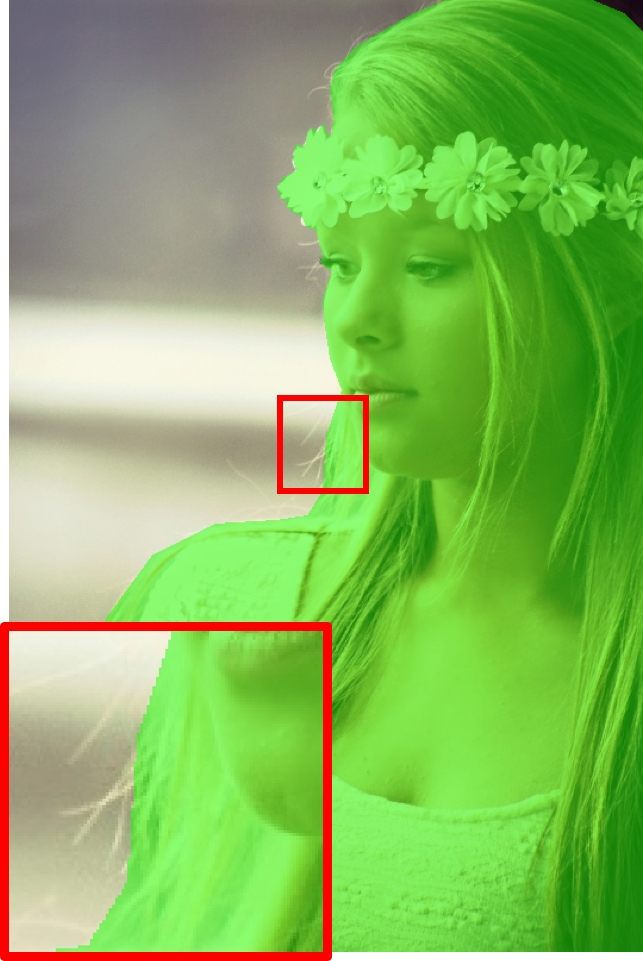
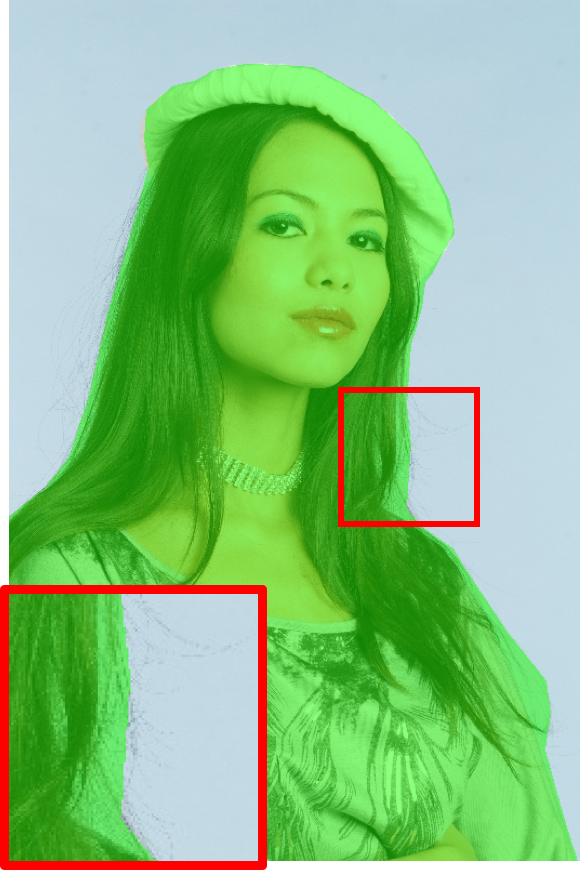
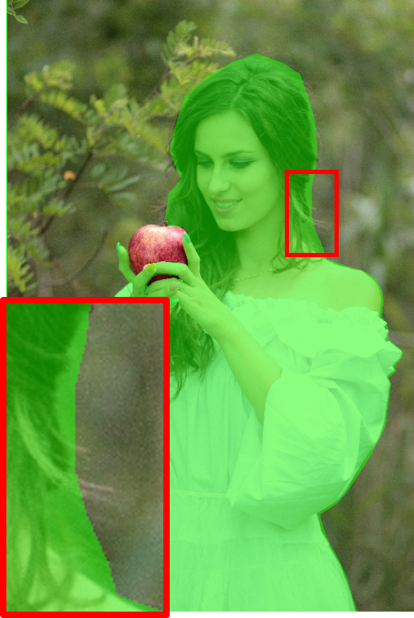
Figure 1: Polygon Annotations of Supervise.ly

(a) Image

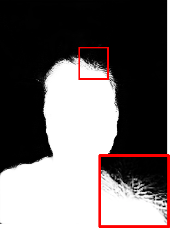
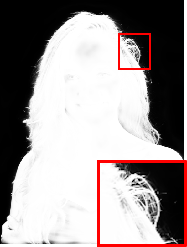
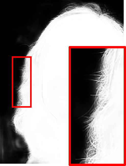
(b) Our Result

(c) Annotation(KNN)

Figure 2: Details of our outputs

In this paper, we propose a specialized portrait segmentation solution by designing BANet. BANet is an efficient network with only 0.62MB parameters, it achieves 43 fps on $512\times 512$ images with high-quality results which are finer than annotations. Some examples are presented in Fig2 . Our experiments show that BANet generates better results than previous portrait segmentation models and real-time segmentation models on PFCN+ dataset.

2 Related Work

Portrait Segmentation Networks: PFCN+[19] provides a benchmark for the task of portrait segmentation. It calculates firstly an average mask from training dataset, then aligns the average mask to each input images to provide prior information. However, the process of alignment requires facial feature points. So, this method needs an additional landmark detection model, which makes the whole process slow and redundant. BSN[8] proposes a boundary-sensitive kernel to take semantic boundary as a third class and it applies many training tricks such as multi-scale training and multi-task learning. However, it still lacks fine details and the inference speed is very slow.

Image Matting Networks: Image matting has been applied for portrait image process for a long time. Traditional matting algorithms [6] [12] [5] [22] require a user defined trimap which limits their applications in automatic image process. Some works [20] [4] have proposed to generate trimap by using deep leaning models, but they still take trimap generation and detail refinement as two separated stages. In matting tasks, trimap helps to locate regions of interest for alpha-matte. Inspired by the function of trimap in matting tasks, we propose a boundary attention mechanism to help our BANet focus on boundary areas. Different from previous matting models, we use a two-branch architecture. Our attention map is generated by high-level semantic branch, and it is used to guide mining low-level features. DIM[23] designs a compositional loss which has been proved to be effective in many matting tasks, but it is time-consuming to prepare large amount of fore-ground, back-ground images and high-quality alpha matte. [13] presents a gradient-coinstency loss which is able to correct gradient direction on prediction edges, but it is not able to extract richer details. Motivated by that, we propose refine loss to obtain richer detail features on boundary area by using image gradient.

High Speed Segmentation Networks: ENet [16] is the first semantic segmentation network that achieves real-time performance. It adopts ResNet [10] bottleneck structure and reduces channel number in order of acceleration, but ENet loses too much accuracy as a tradeoff. ICNet[27] proposes a multi-stream architecture. Three streams extract features from images of different resolution, and then those features are fused by a cascade feature fusion unit. BiSeNet [24] uses a two-stream framework to extract context information and spatial information independently. Then it uses a feature fusion module to combine features of two streams. Inspired by their ideas of separate semantic branch and spatial branch, we design a two-stream architecture. Different from previous works, our two branches are not completely separated. In our framework, low-level branch is guided by high-level branch via a boundary attention map.

Attention Mechanism: Attention mechanism makes high-level information to guide low-level feature extraction. SEnet [11] applies channel attention on image recognition tasks and achieves the state-of-the-art. ExFuse [26] proposes a Semantic Embedding mechanism to use high-level feature to guide low-level feature. DFN [25] learns a global feature as attention to revise the process of feature extraction. In PFCN+ [19], shape channel can be viewed as a kind of spatial-wise attention, aligned mean mask forces model to focus on portrait area.

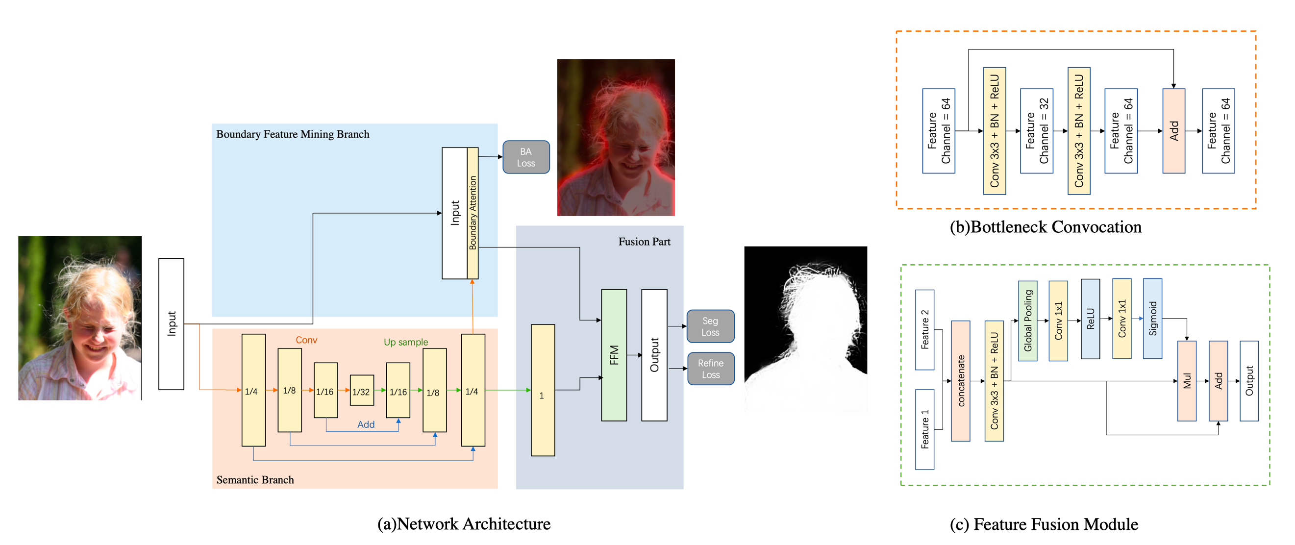
Figure 3: Pipeline of Boundary-Aware Network has three parts. Semantic branch extracts high-level semantic features and produces boundary attention map. Boundary feature mining branch extracts low-level details. Fusion Part fuses high level features and low-level features by a Feature Fusion Module(c). In semantic branch, ResNet bottleneck structure(b) is used as basic convolutional block.

3 Our Method

In the task of portrait segmentation, no-boundary area needs a large receptive field to make prediction with global context information, while boundary area needs small receptive field to focus on local feature contrast. Hence these two areas need to be treated independently. In this paper, we propose a boundary attention mechanism and a weighted loss function to deal with boundary area and no-boundary area separately.

Pipeline of our method is demonstrated as Fig.3. Firstly, color image passes through semantic branch to get 1/4 size high-level semantic features. Secondly, the output of semantic branch is projected into a one-channel feature map and upsampled to full size as boundary attention map. This boundary attention map is supervised by boundary attention loss (BA loss). Then, in boundary feature mining branch, we concatenate input image with the boundary attention map in order to mining low-level features more goal-directed. Lastly, the fusion part fuses high-level semantic features and low-level details to produce fine segmentation results. The final output is supervised by two losses, segmentation loss controls the whole process of portrait segmentation and refine loss refines boundary details.

3.1 Network Architecture

Semantic Branch: The objective of semantic branch is getting a reliable feature representation. This feature representation is dominated by high-level semantic information. At same time, we hope it can contain some spatial information. In the task of portrait segmentation, portrait often occupies a large part of image. Hence, large receptive field is required. Semantic branch is a symmetrical fully convolutional structure that follows FCN-4s structure, we utilize multiple downsampling layers to enlarge the receptive field step by step. As is shown in Fig.3, input image passes through a sequence of convolution layers to get a high-level 1/32 feature map. Then, bilinear interpolation is applied to upsample small scale feature maps. We combine features of 1/16,1/8 and 1/4 scale step by step by elementwise addition. In order to save computation, we use ResNet bottleneck structure as our basic convolutional block, and we fix the max number of channel as 64. The output of semantic branch is a 1/4 size feature map. This feature map has a robust semantic representation because it has large receptive field and it involves 4s level spatial information. More detail information is restorated in Boundary Feature Mining Branch.

Boundary Feature Mining Branch: The output of semantic branch is projected to one channel by $1\times 1$ conv filter, then it is interpolated to full size as boundary attention map. BA loss guides this attention map to locate boundary area. Target of boundary area can be generated without manual annotation. As given in Fig.4. Firstly, we use canny edge detector [2] to extract semantic edges on portrait annotation. Considering portrait area varies a lot in different images, it is not reasonable to dilate each edge to the same width. So, we dilate the edge of different image with different kernel size as follows:

$$K_{dilation}=\frac{S_{portrait}}{S_{portrait}+S_{background}}*W$$ (1)

where W is an empirical value representing the canonical width boundary. In our experiment, we set W = 50.

BA loss is a binary cross-entropy loss, but we don’t want our boundary attention map to be binarized because spatial-wise unsmoothness may cause numerical unstability. Hence, we soften the output of boundary attention map with a Sigmoid function:

$$S(x)=\frac{1}{1+e^{-\frac{x}{T}}}$$ (2)

where T is a temperature which produces a softer probability distribution.

Lastly, input image and attention map are concatenated together as a 4-channel image. This 4-channel image passes through a convolution layer to extract detail information. Different from other multi-stream network architecture that handles each stream independently, our low-level features are guided by high-level features.

Fusion Part: Features of semantic branch and boundary feature mining branch are different in level of feature representation. Therefore, we can’t simplely combine them by element-wise addition nor channel-wise concatenation. In Fusion Part, we follow BiSeNet[24]. Given two features of different levels, we first concatenate them together then we pass them into a sequence of $3\times 3$ convolution, batch normalization and ReLU function. Next, we ulitize global pooling to calculate a weight vector. This vetor helps feature re-weight and feature selection. Fig.3 (b) shows details of Feature Fusion Module.

(a) Portrait Annotation

(b) Boundary Target

(c) Boundary Attention

Figure 4: Boundary Attention

3.2 Loss Function

Our loss function contains three parts as given in Equation 8. Where $L_{seg}$ guides our segmentation results, $L_{bound}$ supervises boundary attention map, and $L_{refine}$ refines boundary details.

Segmentation Loss: Considering the output of portrait segmentation is a one-channel confidence map, binary cross entropy loss is applied as Equation 3. where $y_{p}^{s}$ represents prediction result of segmentation and $y_{t}^{s}$ stands for segmentation target.

$$L_{seg}=-[y_{t}^{s}\cdot log(y_{p}^{s})+(1-y_{t}^{s})\cdot log(1-y_{p}^{s}))]$$ (3)

Boundary Attention Loss: Loss function is the same for the boundary attention map, where $y_{p}^{b}$ means prediction of boundary area. Boundary loss helps our network locate boundary area. At same time, it can be viewed as an intermediate supervision. Extraction of semantic boundary forces the network to learn a feature with strong inter-class distinction ability.

$$L_{bound}=-[y_{t}^{b}\cdot log(y_{p}^{b})+(1-y_{t}^{b})\cdot log(1-y_{p}^{b}))]$$ (4)

Refine Loss : Refine loss is composed by two parts: $L_{cos}$ and $L_{mag}$. The first part $L_{cos}$ uses cosine distance to supervise the gradient direction of segmentation confidence map, $L_{mag}$ brings a constrain on gradient magnitude to inforce the network produce clear and sharp results.

Let $m_{img}$ be the magnitude of gradient of an image, normalized vector $\overrightarrow{\nu}_{img}=(g_{img}^{x},g_{img}^{y})$ denotes the direction of gradient of this image. The output of BAnet is a one-channel confidence map of portrait/background dense classification. Accordingly, we use $m_{pred}$ and $\overrightarrow{\nu}_{pred}$ to represent magnitude and direction of gradient for the output confidence map.

Inspired by [13], a loss measuring the consistency between image gradient and network output is introduced. Our $L_{cos}$ can be formulated as Equation 5.

$$L_{cos} =(1-|\overrightarrow{\nu}_{img}\cdot\overrightarrow{\nu}_{pred}|)\cdot m_{pred}$$ (5)

$$=(1-|g_{img}^{x}\cdot g_{pred}^{x}+g_{img}^{y}\cdot g_{pred}^{y}|)\cdot m_{pred}$$

While $L_{cos}$ can only deal with cases with simple background. When background is confusing, $L_{cos}$ tends to cause blurry prediction boundaries. Different from [13], we add a constrain for gradient magnitude as Equation 6 to force our network to make clear and sharp decision in boundary area. where $\lambda$ is a factor that balances distributional differences between image and output confidence map. In our experiment, $\lambda=1.5$. $L_{mag}$ enables BANet to amplify local contrast when the color of foreground is very similar to background.

$${}L_{mag}=max(\lambda m_{img}-m_{pred},0)$$ (6)

While boundary areas need rich low-level features to obtain detail information, areas far from boundaries are mainly guided by high-level semantic features, too much low-level features will disturb the segmentation result. Therefore, we should combine low-level features selectively. Matting models [23] [4] treat boundary areas and no-boundary areas separately in different stages and then compose two prediction results. Instead of that, BANet has an end-to-end architecture, we use a weighted loss function to distinct boundary area and no-boundary area. As shown in Equation 7 refine loss is only applied in boundary area, where $\mathbb{M}_{bound}$ is a mask which equals 1 only in boundary area. We set $\gamma_{1}=\gamma_{2}=0.5$ in our experiment.

$$L_{refine}=\left(\gamma_{1}L_{cos}+\gamma_{2}L_{mag}\right)\cdot\mathbb{M}_{bound}$$ (7)

Total Loss : Total loss is formulated as a weighted sum of segmentation loss, boundary attention loss and refine loss. Experiments shows $\alpha=0.6,\beta=0.3,\gamma=0.1$ makes good performance.

$$L=\alpha L_{seg}+\beta L_{bound}+\gamma L_{refine}$$ (8)

3.3 Gradient Calculation

$L_{refine}$ needs to calculate image gradient, we design a Gradient Calculation Layer(GCL) to compute image gradient on GPU. Sobel operator [21] is used as convolutional filter in GCL.

$$G_{x}=\left[\begin{array}[]{ccc}+1&0&-1\\ +2&0&-2\\ +1&0&-1\end{array}\right]*I,G_{y}=\left[\begin{array}[]{ccc}+1&+2&+1\\ 0&0&0\\ -1&-2&-1\end{array}\right]*I$$ (9)

where * denotes convolution operation. Gradient magnitude M and gradient vector $\overrightarrow{\nu}$ are computed as follows:

$$M=\sqrt{G_{x}^{2}+G_{y}^{2}}$$ (10)

$$\overrightarrow{\nu}=\left(\frac{G_{x}}{M}\frac{G_{y}}{M}\right)$$ (11)

Considering original image and prediction result have different distribution, before passed through GCL, input is normalized as:

$$I_{norm}=\frac{I-I_{min}}{I_{max}-I_{min}}$$ (12)

Gradient of original image and output confidence map is presented in Fig.5.

(a) Image

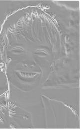
(b) $M_{img}$

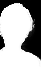
(c) Prediction

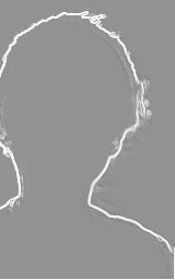
(d) $M_{pred}$

Figure 5: Gradient Calculation

4 Experiment Details

Dataset: PFCN+ [19] dataset contains 1700 KNN annotated portrait images. 1400 images for training and 300 images for test. Supervise.ly contains more than 4000 polygon annotated human segmentation images, but those images are blended by portrait, full-body-shot and multi-person photo. We utilize Supervise.ly dataset to pretrain our model in order to get a better initialization, and then we fine-tune our model on PFCN+ training set, we use PFCN+ test set for evaluation.

Data Augmentation: Online augmentation is implemented during the process of loading data, so that every training sample is unique. Random rotation in range of [-45^∘,45^∘], random flip, random lightness of range [0.7,1.3] are used in order to improve our network’s ability of generalization.

Training Strategy: Considering that $L_{refine}$ is only applied on boundary area, it needs a proper boundary attention map to help locating boundary. Therefore, we firstly pretrain BANet without $L_{refine}$ on Supervise.ly dataset for 40000 iterations to get a good boundary initialization. Then we fine-tune BANet on PFCN+ dataset with $L_{refine}$ for another 40000 iterations.

Supervise.ly dataset and PFCN+ dataset have different data distribution. What’s more, we add $L_{refine}$ during the process of fine-tuning. Hence, it is not appropriate to give a big learning rate at the beginning of fine-tuning. We utilize warming-up learning rate which gives the network a suitable weight initialization before applying big learning rate, thus the network can converge to a better point. Curves of warming-up learning rate can be viewed in Fig.6

Stochastic gradient descent (SGD) optimizer is used to train our model. L2-regularization is applied to all learnable parameters in order to prevent overfitting. Other hyper parameters for training follows Table.1.

Hyper Parameter	Value
Batch Size	16
Weight Decay	$10^{-4}$
Momentum	0.9
Max Learning Rate	0.1
Training Iteration	4 000

Table 1: Hyper Parameter

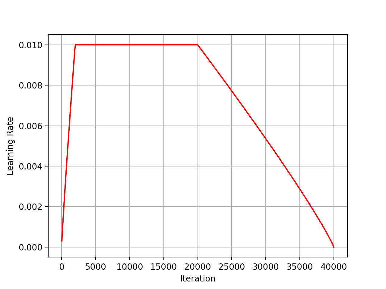
Figure 6: Warming up learning rate

Comparison Experiments: Series of comparison experiments are implemented on some real-time segmentation networks and portrait segmentation networks. For control variates, the same training strategy and hyper parameters are used for all the models. Firstly, these models are pretrained on Supervise.ly dataset, then they get fine-tuned on PFCN+ dataset. Experiment result is demonstrated in Table.2. Mean IoU is measured as criterion of segmentation accuracy. Inference speed is measured on a single GTX 1080 Ti with input size $512\times 512$. Parameter number evaluates the feasibility of implementing these models on edge devices such as mobile phone.

In order to prove our BANet performs better than other portrait segmentation networks with the same order of parameter number, we have also implemented a larger version of BANet with 512 channels, called BANet-512. BANet-64 means the version of BANet with 64 channels.

Result Analysis: As shown in Fig.7. Confidence maps of BiSeNet and EDAnet have vague boundaries, they lack low-level information because they are upsampled directly by bilinear interpolation. PFCN+ has a better semantic representation with the help of prior information provided by shape channel. U-Net get a better boundary because it combines much low-level information. However, U-Net and PFCN+ are still not able to extract fine details like hairs. With the help of boundary attention map and refine loss, BANet-64 is able to produce high-quality results with fine details. In some cases, BANet produces segmentation results which are finer than KNN-annotations. Considering mean IoU measures the similarity between output and annotation, even though PFCN+ and U-Net get a higher mean IoU than BANet-64, we can’t conclude BANet-64 is less accurate than them. While with same order of parameter number, BANet-512 surpasses the other models.

What’s more, PFCN+ has more than 130 MB parameters while our BANet-64 has only 0.62 MB parameters, which makes it possible to be implemented on mobile phone. As for inference speed, BANet-64 achieves 43 FPS on $512\times 512$ images and 115 FPS on $256\times 256$ images, so it can be applied in real-time image processing.

model	mIoU (%)	speed(fps)	parameter(MB)
ENet[16]	88.24	46	0.35
BiSeNet [24]	93.91	59	27.01
EDAnet[14]	94.90	71	0.68
U-Net[18]	95.88	37	13.40
PFCN+[19]	95.92	8	134.27
BANet-64	95.80	43	0.62
BANet-512	96.13	29	12.75

Table 2: Comparison results: All experiments are implemented on Pytorch[17] framework with input images of size $512\times 512$ . Inference speed is measured on a single GTX 1080 Ti.

(a) Image

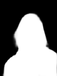
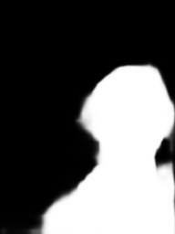
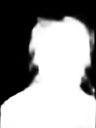
(b) BiSeNet [24]

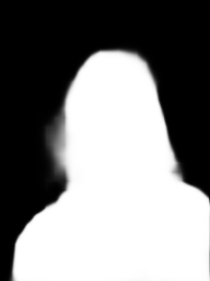
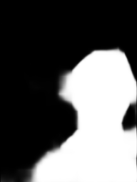
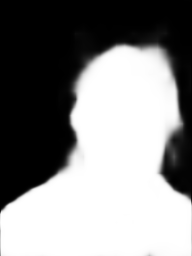
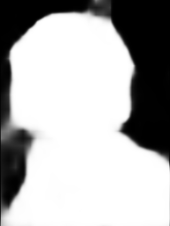
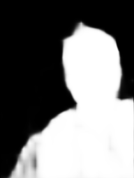
(c) EDAnet [14]

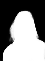
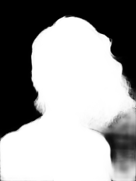
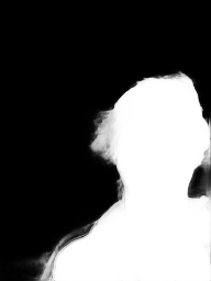
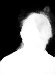
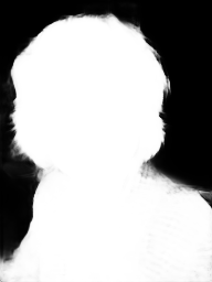
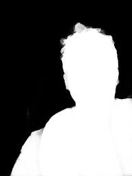
(d) PFCN+ [19]

(e) U-Net [18]

(f) BANet-64

(g) Annotation(KNN)

Figure 7: Comparison results. Traditional Real-time segmentation models like BiSeNet and EDAnet have a huge gap to our work in the task of portrait segmentation. PFCN+ and U-Net have a higher mean IoU than our result but they have obviously coarser boundaries. Mean IoU of our result is limited by target quality.

(a) Image

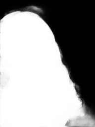
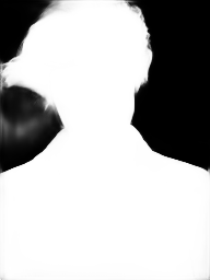
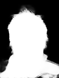
(b) $Ours^{1}$

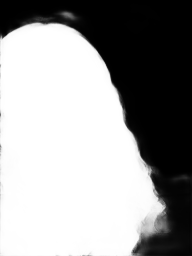
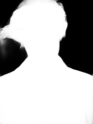
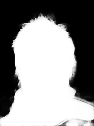
(c) $Ours^{2}$

(d) $Ours^{3}$

Figure 8: Ablation Study shows boundary attention map brings a better semantic prepresentation and refine loss brings finer boundaies.

model	Boundary Attention	Refine Loss	mIoU
Ours1			94.90
Ours2	✓		95.20
Ours3	✓	✓	95.80

• : BANet-64 base model

• : BANet-64 base model + boundary attention

• : BANet-64 base model + boundary attention + refine loss
  

Table 3: Ablation Study

5 Ablation Study

We have also verified the effectiveness of each part in BANet by implementing three versions. $Ours^{1}$ represents BANet base model. In this version, we remove BA loss, refine loss and the little branch of boundary attention map. In boundary feature mining branch, instead of concatenating input image and boundary attention map, we extract low-level features directly on original images. $Ours^{2}$ means BANet with boundary attention map. $Ours^{3}$ stands for BANet with boundary attention map and refine loss. Table 3 shows that boundary attention map and refine loss brings 0.3% and 0.6% improvements respectively. Fig.8 illustrates that boundary attention map brings a better semantic representation and refine loss makes striking enhancement on boundary quality. BANet base model involves low-level feature maps, so it has strong expression ability for details. However, too much low-level feature in no-boundary area may disturb high-level feature representation. Boundary attention map helps BANet focus on boundary area and extract low-level feature selectively. Refine loss enables BANet breaks the limitation of annotation quality to get finer segmentation result.

6 Applications

Our model can be used in mobile applications for real-time selfie processing. We could directly use the output confidence map of BANet as a soft mask for background changing and image beautification. Compared with other algorithm, our model is able to extract finer features with faster speed and less parameters. Some examples are given in Fig.9.

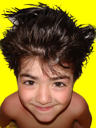
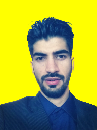
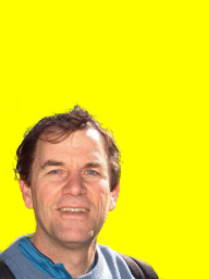
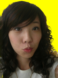
Figure 9: Application on background changing

7 Conclusion and Limitations

In this paper, we propose a Boundary-Aware Network for fast and high-accuracy portrait segmentation. BANet is the first segmentation network that learns to produce results with high-quality boundaries which are finer than annotations. What’s more, light network architecture and high inference speed make it feasible to utilize this model in many practical applications.

As for limitations, in order to make BANet lighter and faster, we have removed too much channels in semantic branch. As a tradeoff, our model’s ability of feature representation is limited. So, BANet has difficulty in learning more complicated cases such as multi-person shot and single person portrait with occlusion.

At present, BANet is trained on only 1400 portrait images, it is far from enough if we want to utilize this model on practical applications. In future works, we will annotate more segmentation targets and we will change backgrounds of existing images to get more training data. With the support of a large training dataset, we will try to apply BANet on mobile phone.

References

- [1] H. Caesar, J. Uijlings, and V. Ferrari. Coco-stuff: Thing and stuff classes in context. CoRR, abs/1612.03716, 5:8, 2016.
- [2] J. Canny. A computational approach to edge detection. IEEE Transactions on pattern analysis and machine intelligence, (6):679--698, 1986.
- [3] L.-C. Chen, G. Papandreou, I. Kokkinos, K. Murphy, and A. L. Yuille. Deeplab: Semantic image segmentation with deep convolutional nets, atrous convolution, and fully connected crfs. IEEE transactions on pattern analysis and machine intelligence, 40(4):834--848, 2018.
- [4] Q. Chen, T. Ge, Y. Xu, Z. Zhang, X. Yang, and K. Gai. Semantic human matting. In 2018 ACM Multimedia Conference on Multimedia Conference, pages 618--626. ACM, 2018.
- [5] Q. Chen, D. Li, and C.-K. Tang. Knn matting. IEEE transactions on pattern analysis and machine intelligence, 35(9):2175--2188, 2013.
- [6] Y.-Y. Chuang, B. Curless, D. H. Salesin, and R. Szeliski. A bayesian approach to digital matting. In null, page 264. IEEE, 2001.
- [7] M. Cordts, M. Omran, S. Ramos, T. Rehfeld, M. Enzweiler, R. Benenson, U. Franke, S. Roth, and B. Schiele. The cityscapes dataset for semantic urban scene understanding. In Proceedings of the IEEE conference on computer vision and pattern recognition, pages 3213--3223, 2016.
- [8] X. Du, X. Wang, D. Li, J. Zhu, S. Tasci, C. Upright, S. Walsh, and L. Davis. Boundary-sensitive network for portrait segmentation. arXiv preprint arXiv:1712.08675, 2017.
- [9] M. Everingham, L. Van Gool, C. K. Williams, J. Winn, and A. Zisserman. The pascal visual object classes (voc) challenge. International journal of computer vision, 88(2):303--338, 2010.
- [10] K. He, X. Zhang, S. Ren, and J. Sun. Deep residual learning for image recognition. In Proceedings of the IEEE conference on computer vision and pattern recognition, pages 770--778, 2016.
- [11] J. Hu, L. Shen, and G. Sun. Squeeze-and-excitation networks. arXiv preprint arXiv:1709.01507, 7, 2017.
- [12] A. Levin, D. Lischinski, and Y. Weiss. A closed-form solution to natural image matting. IEEE transactions on pattern analysis and machine intelligence, 30(2):228--242, 2008.
- [13] A. Levinshtein, C. Chang, E. Phung, I. Kezele, W. Guo, and P. Aarabi. Real-time deep hair matting on mobile devices. CoRR, abs/1712.07168, 2017.
- [14] S.-Y. Lo, H.-M. Hang, S.-W. Chan, and J.-J. Lin. Efficient dense modules of asymmetric convolution for real-time semantic segmentation. arXiv preprint arXiv:1809.06323, 2018.
- [15] J. Long, E. Shelhamer, and T. Darrell. Fully convolutional networks for semantic segmentation. In Proceedings of the IEEE conference on computer vision and pattern recognition, pages 3431--3440, 2015.
- [16] A. Paszke, A. Chaurasia, S. Kim, and E. Culurciello. Enet: A deep neural network architecture for real-time semantic segmentation. arXiv preprint arXiv:1606.02147, 2016.
- [17] A. Paszke, S. Gross, S. Chintala, G. Chanan, E. Yang, Z. DeVito, Z. Lin, A. Desmaison, L. Antiga, and A. Lerer. Automatic differentiation in pytorch. 2017.
- [18] O. Ronneberger, P. Fischer, and T. Brox. U-net: Convolutional networks for biomedical image segmentation. In International Conference on Medical image computing and computer-assisted intervention, pages 234--241. Springer, 2015.
- [19] X. Shen, A. Hertzmann, J. Jia, S. Paris, B. Price, E. Shechtman, and I. Sachs. Automatic portrait segmentation for image stylization. In Computer Graphics Forum, volume 35, pages 93--102. Wiley Online Library, 2016.
- [20] X. Shen, X. Tao, H. Gao, C. Zhou, and J. Jia. Deep automatic portrait matting. In European Conference on Computer Vision, pages 92--107. Springer, 2016.
- [21] I. Sobel. Camera models and machine perception. Technical report, Computer Science Department, Technion, 1972.
- [22] J. Sun, J. Jia, C.-K. Tang, and H.-Y. Shum. Poisson matting. In ACM Transactions on Graphics (ToG), volume 23, pages 315--321. ACM, 2004.
- [23] N. Xu, B. L. Price, S. Cohen, and T. S. Huang. Deep image matting. In CVPR, volume 2, page 4, 2017.
- [24] C. Yu, J. Wang, C. Peng, C. Gao, G. Yu, and N. Sang. Bisenet: Bilateral segmentation network for real-time semantic segmentation. arXiv preprint arXiv:1808.00897, 2018.
- [25] C. Yu, J. Wang, C. Peng, C. Gao, G. Yu, and N. Sang. Learning a discriminative feature network for semantic segmentation. arXiv preprint arXiv:1804.09337, 2018.
- [26] Z. Zhang, X. Zhang, C. Peng, D. Cheng, and J. Sun. Exfuse: Enhancing feature fusion for semantic segmentation. arXiv preprint arXiv:1804.03821, 2018.
- [27] H. Zhao, X. Qi, X. Shen, J. Shi, and J. Jia. Icnet for real-time semantic segmentation on high-resolution images. arXiv preprint arXiv:1704.08545, 2017.
- [28] H. Zhao, J. Shi, X. Qi, X. Wang, and J. Jia. Pyramid scene parsing network. In IEEE Conf. on Computer Vision and Pattern Recognition (CVPR), pages 2881--2890, 2017.
- [29] B. Zhu, Y. Chen, J. Wang, S. Liu, B. Zhang, and M. Tang. Fast deep matting for portrait animation on mobile phone. In Proceedings of the 2017 ACM on Multimedia Conference, pages 297--305. ACM, 2017.