\catchline

One loop correction to $Z\rightarrow\nu\nu$ in the Minimal R-symmetric Supersymmetric Standard Model

Ke-Sheng Sun a,βˆ—    Jian-Bin Chen b,⋆    Xiu-Yi Yang c,†   
Hai-Bin Zhang d,‑
a Department of Physics, Baoding University, Baoding 071000,China
b College of Physics and Optoelectronic Engineering, Taiyuan University of Technology, Taiyuan 030024, China
c School of Science, University of Science and Technology Liaoning, Anshan 114051, China
d Department of Physics, Hebei University, Baoding 071002, China
βˆ— sunkesheng@126.com;sunkesheng@mail.dlut.edu.cn
⋆ chenjianbin@tyut.edu.cn
† yxyruxi@163.com
‑ hbzhang@hbu.edu.cn
Abstract

We analyze the one loop correction to $Z\rightarrow\nu\nu$ decay in framework of Minimal R-symmetric Supersymmetric Standard Model(MRSSM) in detail with normal and inverse neutrino mass orderings, as a function of $\tan\beta$, Dirac mass parameters $M_{D}^{W}$ and $\mu_{u}(\mu_{d})$, slepton mass $m_{l}$ that parameterize the mass matrices. The numerical results indicate that the branching ratio for $Z\rightarrow\nu\nu$ decay is compatible with the experimental measurement and the SM expectation at $2\sigma$ level. For inverse neutrino mass ordering, the prediction exceeds the SM expectation at $1\sigma$ level. The prediction on $Br(Z\rightarrow\nu\nu)$ increases proportionally to $\tan\beta$ and inversely proportionally to $m_{l}$. For normal neutrino mass ordering, the peak value of the prediction on $Br(Z\rightarrow\nu\nu)$ exceeds the SM expectation at $1\sigma$ level.

keywords:
Z boson; MSSM; neutrino.
\pub

Received (Day Month Year)Revised (Day Month Year)

1 Introduction

Invisible decay of Z boson offers constraints on models that lie beyond the Standard Model (SM). The experiment measurement and the SM expectation for the branching ratio of invisible Z-width are [1]

$\displaystyle BR(Z\rightarrow invisible)_{Exp}$ $\displaystyle=$ $\displaystyle 0.2000\pm 0.0006,$ (1)
$\displaystyle BR(Z\rightarrow invisible)_{SM}$ $\displaystyle=$ $\displaystyle 0.2010\pm 0.0001.$ (2)

It shows that the current value of the invisible Z-width in experiment agrees quite well with the SM expectation within $2\sigma$ errors. This is often interpreted as evidence that the SM contains three and only three neutrinos cause, apart from neutrinos, the SM predicts no other channels that these states can decay into. However, there is still a $1\sigma$ level deviation between the experimental measurement and the SM expectation. This departure may hint structures over and above those in the SM.

As a new solution to the supersymmetric flavor problem in MSSM, the Minimal R-symmetric Supersymmetric Standard Model (MRSSM) is proposed in Ref.[2], where the R-symmetry is a fundamental symmetry proposed several decades ago and stronger than R-parity [3, 4]. R-symmetry forbids Majorana gaugino masses, $\mu$ term, $A$ terms and all left-right squark and slepton mass mixings. The $R$-charged Higgs $SU(2)_{L}$ doublets $\hat{R}_{u}$ and $\hat{R}_{d}$ are introduced in MRSSM to yield the Dirac mass terms of higgsinos. Additional superfields $\hat{S}$, $\hat{T}$ and $\hat{O}$ are introduced to yield Dirac mass terms of gauginos. Studies on phenomenology in MRSSM can be found in literatures [5, 6, 7, 8, 9, 10, 11, 12, 13, 14, 15, 16, 17, 18].

In SM, the $Z\rightarrow\nu_{i}\nu_{j}(i=j)$ decays occur at tree level through the interaction between three neutrinos and $Z$ boson

$\displaystyle{\cal L}$ $\displaystyle=$ $\displaystyle C^{Tree}\sum_{i=e,\mu,\tau}\overline{\nu_{i}}\gamma_{\mu}P_{L}\nu_{j}Z^{\mu},$
$\displaystyle C^{Tree}$ $\displaystyle=$ βˆ’12​δi​j​(g1​sW+g2​cW),12superscript𝛿𝑖𝑗subscript𝑔1subscriptπ‘ π‘Šsubscript𝑔2subscriptπ‘π‘Š\displaystyle-\frac{1}{2}\delta^{ij}(g_{1}s_{W}+g_{2}c_{W}),

where sW=s​i​n​θWsubscriptπ‘ π‘Šπ‘ π‘–π‘›subscriptπœƒπ‘Šs_{W}=sin\theta_{W}, cW=c​o​s​θWsubscriptπ‘π‘Šπ‘π‘œπ‘ subscriptπœƒπ‘Šc_{W}=cos\theta_{W} and $\theta_{W}$ is the Weinberg angle, $g_{1}$ denotes the coupling constant of gauge group U(1), $g_{2}$ denotes the coupling constant of gauge group SU(2). At one loop level, the Zβ†’Ξ½i​νj​(iβ‰ j)→𝑍subscriptπœˆπ‘–subscriptπœˆπ‘—π‘–π‘—Z\rightarrow\nu_{i}\nu_{j}(i\neq j) decays arise from the charged current with the mixing among three lepton generations. The fields of the flavor neutrinos in charged current weak interaction Lagrangian are combinations of three massive neutrinos

$\displaystyle{\cal L}$ $\displaystyle=$ $\displaystyle-\frac{g_{2}}{\sqrt{2}}\sum_{l=e,\mu,\tau}\overline{l_{L}}(x)\gamma_{\mu}\nu_{lL}(x)W^{\mu}(x)+h.c.,$
$\displaystyle\nu_{lL}(x)$ $\displaystyle=$ $\displaystyle\sum_{i=1}^{3}\Big{(}U_{PMN}\Big{)}_{li}\nu_{iL}(x),$

where $\nu_{lL}$ are fields of the flavor neutrinos, $\nu_{iL}$ are fields of massive neutrinos, and $U_{PMN}$ corresponds to the unitary neutrino mixing matrix [19, 20]. The unitary neutrino mixing matrix is given by

$\displaystyle U_{PMN}$ $\displaystyle=$ $\displaystyle\left(\begin{array}[]{ccc}c_{1}c_{3}&c_{3}s_{1}&s_{3}e^{-i\delta}\\ -c_{1}s_{3}s_{2}e^{i\delta}-c_{2}s_{1}&c_{1}c_{2}-s_{1}s_{2}s_{3}e^{i\delta}&c_{3}s_{2}\\ s_{1}s_{2}-c_{1}s_{3}c_{2}e^{i\delta}&c_{1}s_{2}-s_{1}c_{2}s_{1}e^{i\delta}&c_{3}c_{2}\end{array}\right)$
$\displaystyle\times diag\Big{(}e^{i\Phi_{1}/2},1,e^{i\Phi_{2}/2}\Big{)},$

where $s(c)_{1}$ = $\sin(\cos)\theta_{12}$, $s(c)_{2}$ = $\sin(\cos)\theta_{23}$, $s(c)_{3}$ = $\sin(\cos)\theta_{13}$. The phase $\delta$ is the Dirac phase, and $\Phi_{i}$ are the Majorana phases.

In this paper, we have studied the $Z\rightarrow\nu\nu$ in MRSSM, where the neutrino mass is assumed with normal ordering and inverse ordering. On one hand, similar to the case in MSSM, the $Z\rightarrow\nu\nu$ decays can arise from the diagrams mediated by charginos $\chi^{\pm}$, neutrinolinos $\chi^{0}$, sleptons $\tilde{L}^{\pm}$ and sneutrinos $\tilde{\nu}$. It is noted worthwhile that the mass matrices in MSSM are different from MRSSM. On the other hand, in MRSSM, the $Z\rightarrow\nu\nu$ decays can also arise from diagrams mediated by another two charginos $\rho^{\pm}$ which have R-charge minus electric charge. Assuming the parameter spaces with two set benchmark points, we investigate the $Z\rightarrow\nu\nu$ decays as functions of $\tan\beta$, Dirac mass parameters $M_{D}^{W}$, $\mu_{u}$, $\mu_{d}$ and slepton mass parameter $m_{l}$ with normal and inverse neutrino mass orderings. The result agrees with the experimental measurement and the SM expectation very well.

The paper is organized as follows. In Section 2, we provide a brief introduction on MRSSM, and derive the analytic expressions for every Feynman diagram contributing to $Z\rightarrow\nu_{i}\nu_{j}$ in MRSSM in detail. The numerical results are presented in Section 3, and the conclusion is drawn in Section 4.

2 MRSSM

The general form of the superpotential of the MRSSM is given by [5]

$\displaystyle\mathcal{W}_{MRSSM}$ $\displaystyle=$ $\displaystyle\mu_{d}(\hat{R}_{d}H_{d})+\mu_{u}(\hat{R}_{u}H_{u})+\Lambda_{d}(\hat{R}_{d}\hat{T})H_{d}+\Lambda_{u}(\hat{R}_{u}\hat{T})H_{u}$ (7)
$\displaystyle+$ $\displaystyle Y_{u}\bar{U}(QH_{u})-Y_{d}\bar{D}(QH_{d})-Y_{e}\bar{E}(LH_{d})$
$\displaystyle+$ $\displaystyle\lambda_{d}\hat{S}(\hat{R}_{d}H_{d})+\lambda_{u}\hat{S}(\hat{R}_{u}H_{u}),$

where $H_{u}$ and $H_{d}$ are the MSSM-like Higgs weak iso-doublets, $\hat{R}_{u}$ and $\hat{R}_{d}$ are the $R$-charged Higgs $SU(2)_{L}$ doublets and the corresponding Dirac higgsino mass parameters are denoted as $\mu_{u}$ and $\mu_{d}$. $\lambda_{u}$, $\lambda_{d}$, $\Lambda_{u}$ and $\Lambda_{d}$ are parameters of Yukawa-like trilinear terms involving the singlet $\hat{S}$ and the triplet $\hat{T}$, which is given by

$$\hat{T}=\left(\begin{array}[]{cc}\hat{T}^{0}/\sqrt{2}&\hat{T}^{+}\\ \hat{T}^{-}&-\hat{T}^{0}/\sqrt{2}\end{array}\right).$$

The soft-breaking scalar mass terms are given by

$\displaystyle V_{SB,S}$ $\displaystyle=$ $\displaystyle m^{2}_{H_{d}}(|H^{0}_{d}|^{2}+|H^{-}_{d}|^{2})+m^{2}_{H_{u}}(|H^{0}_{u}|^{2}+|H^{+}_{u}|^{2})+m^{2}_{R_{u}}(|R^{0}_{u}|^{2}+|R^{-}_{u}|^{2})$ (8)
$\displaystyle+$ $\displaystyle m^{2}_{R_{d}}(|R^{0}_{d}|^{2}+|R^{+}_{d}|^{2})+(B_{\mu}(H^{-}_{d}H^{+}_{u}-H^{0}_{d}H^{0}_{u})+h.c.)$
$\displaystyle+$ $\displaystyle m^{2}_{S}|S|^{2}+m^{2}_{O}|O^{2}|+m^{2}_{T}(|T^{0}|^{2}+|T^{-}|^{2}+|T^{+}|^{2})$
$\displaystyle+$ $\displaystyle\tilde{d}^{*}_{L,i}m_{q,{ij}}^{2}\tilde{d}_{L,j}+\tilde{d}^{*}_{R,i}m_{d,{ij}}^{2}\tilde{d}_{R,j}+\tilde{u}^{*}_{L,i}m_{q,{ij}}^{2}\tilde{u}_{L,j}+\tilde{u}^{*}_{R,i}m_{u,{ij}}^{2}\tilde{u}_{R,j}$
$\displaystyle+$ $\displaystyle\tilde{e}^{*}_{L,i}m_{l,{ij}}^{2}\tilde{e}_{L,j}+\tilde{e}^{*}_{R,{i}}m_{r,{ij}}^{2}\tilde{e}_{R,{j}}+\tilde{\nu}^{*}_{L,i}m_{l,{ij}}^{2}\tilde{\nu}_{L,j}$

All trilinear scalar couplings involving Higgs bosons to squarks and sleptons are forbidden due to the $R$-symmetry. The soft-breaking Dirac mass terms of the singlet $\hat{S}$, triplet $\hat{T}$ and octet $\hat{O}$ take the form

$$V_{SB,DG}=M^{B}_{D}\tilde{B}\tilde{S}+M^{W}_{D}\tilde{W}^{a}\tilde{T}^{a}+M^{O}_{D}\tilde{g}\tilde{O}+h.c.,$$ (9)

where $\tilde{B}$, $\tilde{W}$ and $\tilde{g}$ are usually MSSM Weyl fermions. After EWSB, the mass matrix of four neutralinos $\chi^{0}_{1,2,3,4}$ is given by

$\displaystyle m_{\chi^{0}}$ $\displaystyle=$ $\displaystyle\left(\begin{array}[]{cccc}M^{B}_{D}&0&-\frac{1}{2}g_{1}v_{d}&\frac{1}{2}g_{1}v_{u}\\ 0&M^{W}_{D}&\frac{1}{2}g_{2}v_{d}&-\frac{1}{2}g_{2}v_{u}\\ -\frac{1}{\sqrt{2}}\lambda_{d}v_{d}&-\frac{1}{2}\Lambda_{d}v_{d}&-\mu_{d}^{eff,+}&0\\ \frac{1}{\sqrt{2}}\lambda_{u}v_{u}&-\frac{1}{2}\Lambda_{u}v_{u}&0&\mu_{u}^{eff,-}\end{array}\right),$ (14)

where the modified $\mu_{i}$ parameters are given by

$\displaystyle\mu_{d}^{eff,+}$ $\displaystyle=\frac{1}{2}\Lambda_{d}v_{T}+\frac{1}{\sqrt{2}}\lambda_{d}v_{S}+\mu_{d},$
$\displaystyle\mu_{u}^{eff,-}$ $\displaystyle=-\frac{1}{2}\Lambda_{u}v_{T}+\frac{1}{\sqrt{2}}\lambda_{u}v_{S}+\mu_{u}.$

The $v_{T}$ and $v_{S}$ are vacuum expectation values of $\hat{T}$ and $\hat{S}$ which carry zero $R$-charge. The neutralino mass matrix is diagonalized by unitary matrices $N^{1}$ and $N^{2}$

(N1)βˆ—β€‹mΟ‡0​(N2)†=d​i​a​g​(mΟ‡10,…,mΟ‡40).superscriptsuperscript𝑁1βˆ—subscriptπ‘šsuperscriptπœ’0superscriptsuperscript𝑁2β€ π‘‘π‘–π‘Žπ‘”subscriptπ‘šsubscriptsuperscriptπœ’01…subscriptπ‘šsubscriptsuperscriptπœ’04(N^{1})^{\ast}m_{\chi^{0}}(N^{2})^{\dagger}=diag(m_{\chi^{0}_{1}},...,m_{\chi^{0}_{4}}).

The mass matrix of two charginos $\chi^{\pm}_{1,2}$ with R-charge equal to electric charge is given by

$$m_{\chi^{\pm}}=\left(\begin{array}[]{cc}g_{2}v_{T}+M^{W}_{D}&\frac{1}{\sqrt{2}}\Lambda_{d}v_{d}\\ \frac{1}{\sqrt{2}}g_{2}v_{d}&\mu_{u}^{eff,-}\end{array}\right),$$ (15)

and can be diagonalized by unitary matrices $U^{1}$ and $V^{1}$

(U1)βˆ—β€‹mχ±​(V1)†=d​i​a​g​(mΟ‡1Β±,mΟ‡2Β±).superscriptsuperscriptπ‘ˆ1βˆ—subscriptπ‘šsuperscriptπœ’plus-or-minussuperscriptsuperscript𝑉1β€ π‘‘π‘–π‘Žπ‘”subscriptπ‘šsubscriptsuperscriptπœ’plus-or-minus1subscriptπ‘šsubscriptsuperscriptπœ’plus-or-minus2(U^{1})^{\ast}m_{\chi^{\pm}}(V^{1})^{\dagger}=diag(m_{\chi^{\pm}_{1}},m_{\chi^{\pm}_{2}}).

The mass matrix of two charginos $\rho^{\pm}_{1,2}$ with R-charge equal to minus electric charge is given by

$$m_{\rho^{\pm}}=\left(\begin{array}[]{cc}-g_{2}v_{T}+M^{W}_{D}&\frac{1}{\sqrt{2}}g_{2}v_{u}\\ -\frac{1}{\sqrt{2}}\Lambda_{u}v_{u}&-\mu_{u}^{eff,+}\end{array}\right),$$ (16)

and can be diagonalized by unitary matrices $U^{2}$ and $V^{2}$

(U2)βˆ—β€‹mρ±​(V2)†=d​i​a​g​(mρ1Β±,mρ2Β±).superscriptsuperscriptπ‘ˆ2βˆ—subscriptπ‘šsuperscript𝜌plus-or-minussuperscriptsuperscript𝑉2β€ π‘‘π‘–π‘Žπ‘”subscriptπ‘šsubscriptsuperscript𝜌plus-or-minus1subscriptπ‘šsubscriptsuperscript𝜌plus-or-minus2(U^{2})^{\ast}m_{\rho^{\pm}}(V^{2})^{\dagger}=diag(m_{\rho^{\pm}_{1}},m_{\rho^{\pm}_{2}}).

In the gauge eigenstate basis $\tilde{\nu}_{iL}$, the sneutrino mass squared matrix is expressed as

$$m^{2}_{\tilde{\nu}}=\begin{array}[]{c}m_{l}^{2}+\frac{1}{8}(g_{1}^{2}+g_{2}^{2})(v_{d}^{2}-v_{u}^{2})+g_{2}v_{T}M^{W}_{D}-g_{1}v_{S}M^{B}_{D},\end{array}$$ (17)

where the last two terms are newly introduced by MRSSM, and is diagonalized by unitary matrix $Z^{V}$

ZV​mΞ½~2​(ZV)†=d​i​a​g​(mΞ½~12,mΞ½~22,mΞ½~32).superscript𝑍𝑉subscriptsuperscriptπ‘š2~𝜈superscriptsuperscriptπ‘π‘‰β€ π‘‘π‘–π‘Žπ‘”subscriptsuperscriptπ‘š2subscript~𝜈1subscriptsuperscriptπ‘š2subscript~𝜈2subscriptsuperscriptπ‘š2subscript~𝜈3Z^{V}m^{2}_{\tilde{\nu}}(Z^{V})^{\dagger}=diag(m^{2}_{\tilde{\nu}_{1}},m^{2}_{\tilde{\nu}_{2}},m^{2}_{\tilde{\nu}_{3}}).

The slepton mass squared matrix is given by

$$m^{2}_{\tilde{L}^{\pm}}=\left(\begin{array}[]{cc}(m^{2}_{\tilde{L}^{\pm}})_{LL}&0\\ 0&(m^{2}_{\tilde{L}^{\pm}})_{RR}\end{array}\right),$$ (18)

with

$\displaystyle(m^{2}_{\tilde{L}^{\pm}})_{LL}$ $\displaystyle=m_{l}^{2}+\frac{1}{2}v_{d}^{2}|Y_{e}|^{2}+\frac{1}{8}(g_{1}^{2}-g_{2}^{2})(v_{d}^{2}-v_{u}^{2})-g_{1}v_{S}M_{D}^{B}-g_{2}v_{T}M_{D}^{W},$
$\displaystyle(m^{2}_{\tilde{L}^{\pm}})_{RR}$ $\displaystyle=m_{r}^{2}+\frac{v_{d}^{2}}{2}|Y_{e}|^{2}+\frac{1}{4}g_{1}^{2}(v_{u}^{2}-v_{d}^{2})+2g_{1}v_{S}M_{D}^{B}.$

One can see that the left-right slepton mass mixing is absent. The slepton mass matrix is diagonalized by unitary matrix $Z^{E}$

ZE​mL~Β±2​(ZE)†=d​i​a​g​(mL~1Β±2,…,mL~6Β±2).superscript𝑍𝐸subscriptsuperscriptπ‘š2superscript~𝐿plus-or-minussuperscriptsuperscriptπ‘πΈβ€ π‘‘π‘–π‘Žπ‘”subscriptsuperscriptπ‘š2subscriptsuperscript~𝐿plus-or-minus1…subscriptsuperscriptπ‘š2subscriptsuperscript~𝐿plus-or-minus6Z^{E}m^{2}_{\tilde{L}^{\pm}}(Z^{E})^{\dagger}=diag(m^{2}_{\tilde{L}^{\pm}_{1}},...,m^{2}_{\tilde{L}^{\pm}_{6}}).
Refer to caption
Figure 1: One loop Feynman diagrams contributing to $Z\rightarrow\nu_{i}\nu_{j}$ in MRSSM.

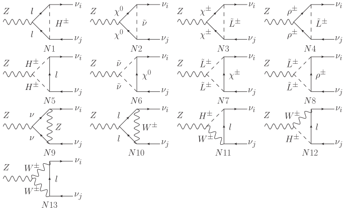
The relevant Feynman diagrams contributing to $Z\rightarrow\nu_{i}\nu_{j}$ in MRSSM is presented in Fig.1. The $Z\nu_{i}\nu_{j}$ interaction Lagrangian can be written as [21]

$\displaystyle\mathcal{L}_{Z\nu_{i}\nu_{j}}=\bar{\nu}_{i}\Big{[}\gamma^{\mu}(C^{1}_{L}P_{L}+C^{1}_{R}P_{R})+p_{1}^{\mu}(C^{2}_{L}P_{L}+C^{2}_{R}P_{R})\Big{]}\nu_{j}Z_{\mu}.$ (19)

Then the branching ratio of LFV decays of $Z$ boson is calculated by

$\displaystyle Br(Z\rightarrow\nu_{i}\nu_{j})$ $\displaystyle=$ $\displaystyle Br(Z\rightarrow\bar{\nu}_{i}\nu_{j})+Br(Z\rightarrow\bar{\nu}_{j}\nu_{i})$ (20)
$\displaystyle=$ $\displaystyle\frac{m_{Z}}{48\pi\Gamma_{Z}}\Big{[}2(|C^{1}_{L}|^{2}+|C^{1}_{R}|^{2})+\frac{m_{Z}^{2}}{4}(|C^{2}_{L}|^{2}+|C^{2}_{R}|^{2})\Big{]},$

where the neutrino masses have been neglected and $\Gamma_{Z}$ is the total decay width of $Z$ boson. For convenience, following notation is used

$\displaystyle Br(Z\rightarrow\nu\nu)=\sum_{i,j=1,2,3}Br(Z\rightarrow\nu_{i}\nu_{j}),i\leq j.$

The coefficients $C^{1}_{L/R}$ and $C^{2}_{L/R}$ are combinations of coefficients corresponding to each Feynman diagram in Fig.1

$\displaystyle C^{1}_{L}$ $\displaystyle=$ $\displaystyle C^{Tree}+\sum_{N=N1}^{N13}C^{1,N}_{L},$
$\displaystyle C^{1}_{R}$ $\displaystyle=$ $\displaystyle\sum_{N=N1}^{N13}C^{1,N}_{R},$
$\displaystyle C^{2}_{L/R}$ $\displaystyle=$ $\displaystyle\sum_{N=N1}^{N13}C^{2,N}_{L/R}.$

Actually, only $C^{1,N}_{L}$ contribute to the decay width cause other coefficients $C^{1,N}_{R}$ and $C^{2,N}_{L/R}$ equal zero. The explicit expressions of $C^{1,N}_{L}$ are derived by assuming the three neutrino masses are zero in terms of invariant Passarino-Veltman integrals [22]. The coefficients $C^{1,N}_{L}$ in Fig.1 (N1-N4) are calculated by

$\displaystyle C^{1,N}_{L}=C^{N}_{1R}C^{N}_{3L}(C^{N}_{2R}\mathcal{B}_{0}(m_{Z}^{2},M_{1},M_{2})+(C^{N}_{2L}M_{1}M_{2}+C^{N}_{2R}M_{3}^{2})\mathcal{C}_{0}-2C^{N}_{2R}\mathcal{C}_{00}),$

where

$\displaystyle C^{N1}_{1R}$ $\displaystyle=$ Yli​Zn​1+,C2​LN​1=Ξ΄i​j2​(g2​cWβˆ’g1​sW),C2​RN​1=βˆ’g1​sW​δi​j,formulae-sequencesubscriptsuperscriptπ‘Œπ‘–π‘™subscriptsuperscript𝑍𝑛1subscriptsuperscript𝐢𝑁12𝐿superscript𝛿𝑖𝑗2subscript𝑔2subscriptπ‘π‘Šsubscript𝑔1subscriptπ‘ π‘Šsubscriptsuperscript𝐢𝑁12𝑅subscript𝑔1subscriptπ‘ π‘Šsuperscript𝛿𝑖𝑗\displaystyle Y^{i}_{l}Z^{+}_{n1},C^{N1}_{2L}=\frac{\delta^{ij}}{2}(g_{2}c_{W}-g_{1}s_{W}),C^{N1}_{2R}=-g_{1}s_{W}\delta^{ij},
$\displaystyle C^{N1}_{3L}$ $\displaystyle=$ $\displaystyle Y^{j}_{l}Z^{+}_{n1},M_{1}=m_{l_{k}},M_{2}=m_{l_{m}},M_{3}=m_{H^{\pm}_{n}},(N=N1),$
$\displaystyle C^{N2}_{1R}$ $\displaystyle=$ $\displaystyle\frac{1}{\sqrt{2}}Z^{V,\ast}_{ni}(g_{1}N^{1}_{k1}-g_{2}N^{1}_{k2}),C^{N2}_{3L}=\frac{1}{\sqrt{2}}Z^{V}_{nj}(g_{1}N^{1,\ast}_{m1}-g_{2}N^{1,\ast}_{m2}),$
$\displaystyle C^{N2}_{2L}$ $\displaystyle=$ 12​(g2​cW+g1​sW)​(Nk​32,βˆ—β€‹Nm​32,βˆ—βˆ’Nk​42,βˆ—β€‹Nm​42,βˆ—),12subscript𝑔2subscriptπ‘π‘Šsubscript𝑔1subscriptπ‘ π‘Šsubscriptsuperscript𝑁2βˆ—π‘˜3subscriptsuperscript𝑁2βˆ—π‘š3subscriptsuperscript𝑁2βˆ—π‘˜4subscriptsuperscript𝑁2βˆ—π‘š4\displaystyle\frac{1}{2}(g_{2}c_{W}+g_{1}s_{W})(N^{2,\ast}_{k3}N^{2,\ast}_{m3}-N^{2,\ast}_{k4}N^{2,\ast}_{m4}),
$\displaystyle C^{N2}_{2R}$ $\displaystyle=$ 12​(g2​cW+g1​sW)​(Nm​31,βˆ—β€‹Nk​31,βˆ—βˆ’Nm​41,βˆ—β€‹Nk​42,βˆ—),12subscript𝑔2subscriptπ‘π‘Šsubscript𝑔1subscriptπ‘ π‘Šsubscriptsuperscript𝑁1βˆ—π‘š3subscriptsuperscript𝑁1βˆ—π‘˜3subscriptsuperscript𝑁1βˆ—π‘š4subscriptsuperscript𝑁2βˆ—π‘˜4\displaystyle\frac{1}{2}(g_{2}c_{W}+g_{1}s_{W})(N^{1,\ast}_{m3}N^{1,\ast}_{k3}-N^{1,\ast}_{m4}N^{2,\ast}_{k4}),
$\displaystyle M_{1}$ $\displaystyle=$ $\displaystyle m_{\chi^{0}_{k}},M_{2}=m_{\chi^{0}_{m}},M_{3}=m_{\tilde{\nu}_{n}},(N=N2),$

and

$\displaystyle C^{N3}_{1R}$ $\displaystyle=$ Yli​Zn​(3+i)E,βˆ—β€‹Uk​21,C2​LN​3=βˆ’12​(2​g2​cW​Vm​11,βˆ—β€‹Vk​11+(g2​cWβˆ’g1​sW)​Vm​21,βˆ—β€‹Vk​21),subscriptsuperscriptπ‘Œπ‘–π‘™subscriptsuperscriptπ‘πΈβˆ—π‘›3𝑖subscriptsuperscriptπ‘ˆ1π‘˜2subscriptsuperscript𝐢𝑁32𝐿122subscript𝑔2subscriptπ‘π‘Šsubscriptsuperscript𝑉1βˆ—π‘š1subscriptsuperscript𝑉1π‘˜1subscript𝑔2subscriptπ‘π‘Šsubscript𝑔1subscriptπ‘ π‘Šsubscriptsuperscript𝑉1βˆ—π‘š2subscriptsuperscript𝑉1π‘˜2\displaystyle Y^{i}_{l}Z^{E,\ast}_{n(3+i)}U^{1}_{k2},C^{N3}_{2L}=-\frac{1}{2}(2g_{2}c_{W}V^{1,\ast}_{m1}V^{1}_{k1}+(g_{2}c_{W}-g_{1}s_{W})V^{1,\ast}_{m2}V^{1}_{k2}),
$\displaystyle C^{N3}_{2R}$ $\displaystyle=$ βˆ’12​(2​g2​cW​Uk​11,βˆ—β€‹Um​11+(g2​cWβˆ’g1​sW)​Uk​21,βˆ—β€‹Um​21),122subscript𝑔2subscriptπ‘π‘Šsubscriptsuperscriptπ‘ˆ1βˆ—π‘˜1subscriptsuperscriptπ‘ˆ1π‘š1subscript𝑔2subscriptπ‘π‘Šsubscript𝑔1subscriptπ‘ π‘Šsubscriptsuperscriptπ‘ˆ1βˆ—π‘˜2subscriptsuperscriptπ‘ˆ1π‘š2\displaystyle-\frac{1}{2}(2g_{2}c_{W}U^{1,\ast}_{k1}U^{1}_{m1}+(g_{2}c_{W}-g_{1}s_{W})U^{1,\ast}_{k2}U^{1}_{m2}),
$\displaystyle C^{N3}_{3L}$ $\displaystyle=$ $\displaystyle Y^{j}_{l}Z^{E}_{n(3+j)}U^{1,\ast}_{m2},M_{1}=m_{\chi^{\pm}_{k}},M_{2}=m_{\chi^{\pm}_{m}},M_{3}=m_{\tilde{L}^{\pm}_{n}},(N=N3),$
$\displaystyle C^{N4}_{1R}$ $\displaystyle=$ βˆ’g2​Zn​iE,βˆ—β€‹Uk​12,C2​LN​4=12​(2​g2​cW​Vm​12,βˆ—β€‹Vk​12,βˆ—+(g2​cWβˆ’g1​sW)​Vm​22,βˆ—β€‹Vk​22),subscript𝑔2subscriptsuperscriptπ‘πΈβˆ—π‘›π‘–subscriptsuperscriptπ‘ˆ2π‘˜1subscriptsuperscript𝐢𝑁42𝐿122subscript𝑔2subscriptπ‘π‘Šsubscriptsuperscript𝑉2βˆ—π‘š1subscriptsuperscript𝑉2βˆ—π‘˜1subscript𝑔2subscriptπ‘π‘Šsubscript𝑔1subscriptπ‘ π‘Šsubscriptsuperscript𝑉2βˆ—π‘š2subscriptsuperscript𝑉2π‘˜2\displaystyle-g_{2}Z^{E,\ast}_{ni}U^{2}_{k1},C^{N4}_{2L}=\frac{1}{2}(2g_{2}c_{W}V^{2,\ast}_{m1}V^{2,\ast}_{k1}+(g_{2}c_{W}-g_{1}s_{W})V^{2,\ast}_{m2}V^{2}_{k2}),
$\displaystyle C^{N4}_{2R}$ $\displaystyle=$ 12​(2​g2​cW​Uk​12,βˆ—β€‹Um​12,βˆ—+(g2​cWβˆ’g1​sW)​Uk​12,βˆ—β€‹Um​12),C3​LN​4=βˆ’g2​Um​12,βˆ—β€‹Zn​jE,122subscript𝑔2subscriptπ‘π‘Šsubscriptsuperscriptπ‘ˆ2βˆ—π‘˜1subscriptsuperscriptπ‘ˆ2βˆ—π‘š1subscript𝑔2subscriptπ‘π‘Šsubscript𝑔1subscriptπ‘ π‘Šsubscriptsuperscriptπ‘ˆ2βˆ—π‘˜1subscriptsuperscriptπ‘ˆ2π‘š1subscriptsuperscript𝐢𝑁43𝐿subscript𝑔2subscriptsuperscriptπ‘ˆ2βˆ—π‘š1subscriptsuperscript𝑍𝐸𝑛𝑗\displaystyle\frac{1}{2}(2g_{2}c_{W}U^{2,\ast}_{k1}U^{2,\ast}_{m1}+(g_{2}c_{W}-g_{1}s_{W})U^{2,\ast}_{k1}U^{2}_{m1}),C^{N4}_{3L}=-g_{2}U^{2,\ast}_{m1}Z^{E}_{nj},
$\displaystyle M_{1}$ $\displaystyle=$ $\displaystyle m_{\rho^{\pm}_{k}},M_{2}=m_{\rho^{\pm}_{m}},M_{3}=m_{\tilde{L}^{\pm}_{n}},(N=N4).$

The coefficients $C^{1,N}_{L}$ in Fig.1 (N5-N8) are calculated by

$\displaystyle C^{1,N}_{L}=2C^{N}_{1R}C^{N}_{2}C^{N}_{3L}\mathcal{C}_{00},$

where

$\displaystyle C^{N5}_{1R}$ $\displaystyle=$ $\displaystyle Y^{i}_{l}Z^{+}_{k1},C^{N5}_{3L}=Y^{j}_{l}Z^{+}_{m1},$
$\displaystyle C^{N5}_{2}$ $\displaystyle=$ 12​((g2​cWβˆ’g1​sW)​(Zk​1+​Zm​1++Zk​2+​Zm​2+)+2​g2​cW​(Zk​3+​Zm​3++Zk​4+​Zm​4+)),12subscript𝑔2subscriptπ‘π‘Šsubscript𝑔1subscriptπ‘ π‘Šsubscriptsuperscriptπ‘π‘˜1subscriptsuperscriptπ‘π‘š1subscriptsuperscriptπ‘π‘˜2subscriptsuperscriptπ‘π‘š22subscript𝑔2subscriptπ‘π‘Šsubscriptsuperscriptπ‘π‘˜3subscriptsuperscriptπ‘π‘š3subscriptsuperscriptπ‘π‘˜4subscriptsuperscriptπ‘π‘š4\displaystyle\frac{1}{2}((g_{2}c_{W}-g_{1}s_{W})(Z^{+}_{k1}Z^{+}_{m1}+Z^{+}_{k2}Z^{+}_{m2})+2g_{2}c_{W}(Z^{+}_{k3}Z^{+}_{m3}+Z^{+}_{k4}Z^{+}_{m4})),
$\displaystyle M_{1}$ $\displaystyle=$ $\displaystyle m_{H^{\pm}_{k}},M_{2}=m_{H^{\pm}_{m}},M_{3}=m_{l_{n}},(N=N5),$
$\displaystyle C^{N6}_{1R}$ $\displaystyle=$ $\displaystyle\frac{1}{\sqrt{2}}Z^{V,\ast}_{ki}(g_{1}N^{1}_{n1}-g_{2}N^{1}_{n2}),C^{N6}_{3L}=\frac{1}{\sqrt{2}}Z^{V}_{mj}(g_{1}N^{1,\ast}_{n1}-g_{2}N^{1,\ast}_{n2}),$
$\displaystyle C^{N6}_{2}$ $\displaystyle=$ βˆ’12​δk​m​(g1​sW+g2​cW),M1=mΞ½~k,M2=mΞ½~m,M3=mΟ‡nΒ±,(N=N​6),formulae-sequence12superscriptπ›Ώπ‘˜π‘šsubscript𝑔1subscriptπ‘ π‘Šsubscript𝑔2subscriptπ‘π‘Šsubscript𝑀1subscriptπ‘šsubscript~πœˆπ‘˜formulae-sequencesubscript𝑀2subscriptπ‘šsubscript~πœˆπ‘šsubscript𝑀3subscriptπ‘šsubscriptsuperscriptπœ’plus-or-minus𝑛𝑁𝑁6\displaystyle-\frac{1}{2}\delta^{km}(g_{1}s_{W}+g_{2}c_{W}),M_{1}=m_{\tilde{\nu}_{k}},M_{2}=m_{\tilde{\nu}_{m}},M_{3}=m_{\chi^{\pm}_{n}},(N=N6),

and

$\displaystyle C^{N7}_{1R}$ $\displaystyle=$ $\displaystyle Y^{i}_{l}Z^{E,\ast}_{k(3+i)}U^{1}_{n2},C^{N7}_{3L}=Y^{j}_{l}Z^{E}_{m(3+j)}U^{1,\ast}_{n2},$
$\displaystyle C^{N7}_{2}$ $\displaystyle=$ βˆ‘a=1,2,312​(βˆ’2​g1​sW​Zm​(3+a)E,βˆ—β€‹Zk​(3+a)E+(g2​cWβˆ’g1​sW)​Zm​aE,βˆ—β€‹Zk​aE),subscriptπ‘Ž123122subscript𝑔1subscriptπ‘ π‘Šsubscriptsuperscriptπ‘πΈβˆ—π‘š3π‘Žsubscriptsuperscriptπ‘πΈπ‘˜3π‘Žsubscript𝑔2subscriptπ‘π‘Šsubscript𝑔1subscriptπ‘ π‘Šsubscriptsuperscriptπ‘πΈβˆ—π‘šπ‘Žsubscriptsuperscriptπ‘πΈπ‘˜π‘Ž\displaystyle\sum_{a=1,2,3}\frac{1}{2}(-2g_{1}s_{W}Z^{E,\ast}_{m(3+a)}Z^{E}_{k(3+a)}+(g_{2}c_{W}-g_{1}s_{W})Z^{E,\ast}_{ma}Z^{E}_{ka}),
$\displaystyle M_{1}$ $\displaystyle=$ $\displaystyle m_{\tilde{L}^{\pm}_{k}},M_{2}=m_{\tilde{L}^{\pm}_{m}},M_{3}=\chi^{\pm}_{n},(N=N7),$
$\displaystyle C^{N8}_{1R}$ $\displaystyle=$ $\displaystyle-g_{2}Z^{E,\ast}_{ki}U^{2}_{n1},C^{N8}_{3L}=-g_{2}Z^{E}_{mj}U^{2,\ast}_{n1},$
$\displaystyle C^{N8}_{2}$ $\displaystyle=$ βˆ‘a=1,2,312​(βˆ’2​g1​sW​Zm​(3+a)E,βˆ—β€‹Zk​(3+a)E+(g2​cWβˆ’g1​sW)​Zm​aE,βˆ—β€‹Zk​aE),subscriptπ‘Ž123122subscript𝑔1subscriptπ‘ π‘Šsubscriptsuperscriptπ‘πΈβˆ—π‘š3π‘Žsubscriptsuperscriptπ‘πΈπ‘˜3π‘Žsubscript𝑔2subscriptπ‘π‘Šsubscript𝑔1subscriptπ‘ π‘Šsubscriptsuperscriptπ‘πΈβˆ—π‘šπ‘Žsubscriptsuperscriptπ‘πΈπ‘˜π‘Ž\displaystyle\sum_{a=1,2,3}\frac{1}{2}(-2g_{1}s_{W}Z^{E,\ast}_{m(3+a)}Z^{E}_{k(3+a)}+(g_{2}c_{W}-g_{1}s_{W})Z^{E,\ast}_{ma}Z^{E}_{ka}),
$\displaystyle M_{1}$ $\displaystyle=$ $\displaystyle m_{\tilde{L}^{\pm}_{k}},M_{2}=m_{\tilde{L}^{\pm}_{m}},M_{3}=m_{\rho^{\pm}_{n}},(N=N8).$

The coefficients $C^{1,N}_{L}$ in Fig.1 (N9-N10) are calculated by

$\displaystyle C^{1,N}_{L}$ $\displaystyle=$ $\displaystyle-2C^{N}_{1L}C^{N}_{3L}(-C^{N}_{2L}\mathcal{B}_{0}(m_{Z}^{2},M_{1},M_{2})+C^{N}_{2L}(\mathcal{B}_{0}(0,M_{3},M_{1})+\mathcal{B}_{0}(0,M_{3},M_{2}))$
$\displaystyle+$ $\displaystyle C^{N}_{2L}(M_{1}^{2}+M_{2}^{2}-M_{3}^{2}-m_{Z}^{2})\mathcal{C}_{0}+C^{N}_{2R}M_{1}M_{2}\mathcal{C}_{0}-2C^{N}_{2L}\mathcal{C}_{00}),$

where

$\displaystyle C^{N9}_{1L}$ $\displaystyle=$ βˆ’Ξ΄k​i2​(g1​sW+g2​cW),C2​LN​9=βˆ’Ξ΄k​m2​(g1​sW+g2​cW),C2​RN​9=0,formulae-sequencesuperscriptπ›Ώπ‘˜π‘–2subscript𝑔1subscriptπ‘ π‘Šsubscript𝑔2subscriptπ‘π‘Šsubscriptsuperscript𝐢𝑁92𝐿superscriptπ›Ώπ‘˜π‘š2subscript𝑔1subscriptπ‘ π‘Šsubscript𝑔2subscriptπ‘π‘Šsubscriptsuperscript𝐢𝑁92𝑅0\displaystyle-\frac{\delta^{ki}}{2}(g_{1}s_{W}+g_{2}c_{W}),C^{N9}_{2L}=-\frac{\delta^{km}}{2}(g_{1}s_{W}+g_{2}c_{W}),C^{N9}_{2R}=0,
$\displaystyle C^{N9}_{3L}$ $\displaystyle=$ βˆ’Ξ΄m​j2​(g1​sW+g2​cW),M1=0,M2=0,M3=mZ,(N=N​9),formulae-sequencesuperscriptπ›Ώπ‘šπ‘—2subscript𝑔1subscriptπ‘ π‘Šsubscript𝑔2subscriptπ‘π‘Šsubscript𝑀10formulae-sequencesubscript𝑀20subscript𝑀3subscriptπ‘šπ‘π‘π‘9\displaystyle-\frac{\delta^{mj}}{2}(g_{1}s_{W}+g_{2}c_{W}),M_{1}=0,M_{2}=0,M_{3}=m_{Z},(N=N9),
$\displaystyle C^{N10}_{1L}$ $\displaystyle=$ βˆ’g22​(UP​M​Nβˆ—)k​i,C2​LN​10=Ξ΄k​m2​(g2​cWβˆ’g1​sW),C2​RN​10=βˆ’Ξ΄k​m​g1​sW,formulae-sequencesubscript𝑔22subscriptsubscriptsuperscriptπ‘ˆβˆ—π‘ƒπ‘€π‘π‘˜π‘–subscriptsuperscript𝐢𝑁102𝐿superscriptπ›Ώπ‘˜π‘š2subscript𝑔2subscriptπ‘π‘Šsubscript𝑔1subscriptπ‘ π‘Šsubscriptsuperscript𝐢𝑁102𝑅superscriptπ›Ώπ‘˜π‘šsubscript𝑔1subscriptπ‘ π‘Š\displaystyle-\frac{g_{2}}{\sqrt{2}}(U^{\ast}_{PMN})_{ki},C^{N10}_{2L}=\frac{\delta^{km}}{2}(g_{2}c_{W}-g_{1}s_{W}),C^{N10}_{2R}=-\delta^{km}g_{1}s_{W},
$\displaystyle C^{N10}_{3L}$ $\displaystyle=$ $\displaystyle-\frac{g_{2}}{\sqrt{2}}(U_{PMN})_{mj},M_{1}=m_{l_{k}},M_{2}=m_{l_{m}},M_{3}=m_{W},(N=N10).$

The coefficients $C^{1,N}_{L}$ in Fig.1 (N11-N12) are calculated by

$\displaystyle C^{1,N}_{L}$ $\displaystyle=$ $\displaystyle C^{N}_{1}C^{N}_{2}C^{N}_{3}\mathcal{C}_{0},$

where

$\displaystyle C^{N11}_{1}$ $\displaystyle=$ $\displaystyle Y^{i}_{l}Z^{+}_{k1},C^{N11}_{3}=-\frac{g_{2}}{\sqrt{2}}(U_{PMN})_{nj},$
$\displaystyle C^{N11}_{2}$ $\displaystyle=$ $\displaystyle-\frac{g_{2}}{2}(-g_{1}v_{d}s_{W}Z^{+}_{k1}+g_{1}v_{u}s_{W}Z^{+}_{k2}+\sqrt{2}g_{2}v_{T}c_{W}(Z^{+}_{k3}+Z^{+}_{k4}),$
$\displaystyle M_{1}$ $\displaystyle=$ $\displaystyle m_{H^{\pm}_{k}},M_{2}=m_{W},M_{3}=m_{l_{n}},(N=N11),$
$\displaystyle C^{N12}_{1}$ $\displaystyle=$ $\displaystyle-\frac{g_{2}}{\sqrt{2}}(U^{\ast}_{PMN})_{ki},C^{N12}_{3}=Y^{j}_{l}Z^{+}_{m1},$
$\displaystyle C^{N12}_{2}$ $\displaystyle=$ $\displaystyle-\frac{g_{2}}{2}(-g_{1}v_{d}s_{W}Z^{+}_{m1}+g_{1}v_{u}s_{W}Z^{+}_{m2}+\sqrt{2}g_{2}v_{T}c_{W}(Z^{+}_{m3}+Z^{+}_{m4}),$
$\displaystyle M_{1}$ $\displaystyle=$ $\displaystyle m_{W},M_{2}=m_{H^{\pm}_{m}},M_{3}=m_{l_{n}},(N=N12).$

The coefficients $C^{1,N}_{L}$ in Fig.1 (N13) are calculated by

$\displaystyle C^{1,N}_{L}$ $\displaystyle=$ $\displaystyle 2C^{N}_{1}C^{N}_{2}C^{N}_{3}(\mathcal{B}_{0}(m_{Z}^{2},M_{1},M_{2})+M_{3}^{2}\mathcal{C}_{0}+2\mathcal{C}_{00}),$

where

$\displaystyle C^{N13}_{1}$ $\displaystyle=$ $\displaystyle-\frac{g_{2}}{\sqrt{2}}(U^{\ast}_{PMN})_{ni},C^{N13}_{2}=-g_{2}c_{W},C^{N13}_{3}=-\frac{g_{2}}{\sqrt{2}}(U_{PMN})_{nj},$
$\displaystyle M_{1}$ $\displaystyle=$ $\displaystyle m_{W},M_{2}=m_{W},M_{3}=m_{l_{n}},(N=N13).$

The loop integrals are given in term of Passarino-Veltman [22]

$\displaystyle\mathcal{C}_{(0,00)}$ $\displaystyle=$ $\displaystyle\frac{i}{16\pi^{2}}\mathcal{C}_{(0,00)}(0,m_{Z}^{2},0;M_{3},M_{1},M_{2}).$

The explicit expressions of these loop integrals are given in Refs [23, 24, 25] and $\overline{MS}$ scheme is used to delete the infinite terms. These loop integrals can be calculated through the Mathematica package Package-X [26] and a link to Collier which is a fortran library for the numerical evaluation of one-loop scalar and tensor integrals[27].

3 Numerical Analysis

In the numerical analysis, we use the two set benchmark points taken from existing references as the default values for our parameter setup and display them in Table.3 [7], where the slepton mass matrices are diagonal and all mass parameters are in $GeV$ or $GeV^{2}$. The following numerical values are used

$\displaystyle\alpha_{em}(m_{Z})=1/128,m_{Z}=91.1876GeV,m_{W}=80.379GeV,\Gamma_{Z}=2.49GeV,$
$\displaystyle sin^{2}\theta_{W}=0.23129,m_{e}=0.510MeV,m_{\mu}=105.6MeV,m_{\tau}=1.776GeV.$

The light neutrino mass spectrum is assumed to be normal ordering, the best-fit values of the three neutrino oscillation parameters are given in Table.3.

\tbl

The best-fit values correspond to normal ordering(NO) and inverse ordering(IO). \topruleParameter best-fit(NO) best-fit(IO) Parameter best-fit(NO) best-fit(IO) \colrule$sin^{2}\theta_{12}$ 0.297 0.297 $sin^{2}\theta_{23}$ 0.425 0.589 $sin^{2}\theta_{13}$ 0.0215 0.0216 $\delta$ 1.38$\pi$ 1.38$\pi$ \botrule

Apart from the above result, no other experimental information on the Majorana phases in the neutrino mixing matrix is available at present. Note that large value of $|v_{T}|$ is excluded by measurement of $W$ mass cause the vev $v_{T}$ of the $SU(2)_{L}$ triplet field $T^{0}$ gives a correction to $W$ mass through [5]

$\displaystyle m_{W}^{2}=\frac{1}{4}g_{2}^{2}v^{2}+g_{2}^{2}v_{T}^{2},$ (21)

with $v^{2}=v_{u}^{2}+v_{d}^{2}$.

\tbl

Benchmark points. \topruleInput $tan\beta$ $\lambda_{d}$,$\lambda_{u}$ $\Lambda_{d}$,$\Lambda_{u}$ $v_{S}$ $v_{T}$ $M_{D}^{B}$ $M_{D}^{W}$ $\mu_{d}$,$\mu_{u}$ $m_{T}^{2}$ $m^{2}_{l}$,$m_{r}^{2}$ \colruleBMP1 10 1.1,-1.1 -1.0,-1.0 1.3 -0.19 1000 500 400,400 $3000^{2}$ $1000^{2}$,$1000^{2}$ \colruleBMP2 40 0.15,-0.15 -1.0,-1.15 -0.14 -0.34 250 500 400,400 $3000^{2}$ $1000^{2}$,$1000^{2}$ \botrule

Refer to caption
Figure 2: The $Br(Z\rightarrow\nu\nu)$ vary as a function of $tan\beta$ in MRSSM, where the solid line (BMP1) and the dash dot line (BMP2) correspond to normal neutrino mass ordering, the dot line (BMP1) and the dash line (BMP2) correspond to inverse neutrino mass ordering and the two lines are almost identical.

In Fig.2, we display the theoretical prediction of $Br(Z\rightarrow\nu\nu)$ versus $tan\beta$ in MRSSM. The solid line and the dot line stand for the result calculated with parameter setup BMP1 with normal ordering and inverse ordering respectively. The dash dot line and the dash line stand for the result calculated with parameter setup BMP2 with normal ordering and inverse ordering respectively. Both predictions increase along with $tan\beta$ and are compatible with the experimental measurement at $2\sigma$ level. For normal ordering , the prediction of $Br(Z\rightarrow\nu\nu)$ with BMP1 is a little lower than that with BMP2. For inverse ordering, the predictions are almost identical. At $1\sigma$ level, the prediction of $Br(Z\rightarrow\nu\nu)$ with normal ordering is compatible with the SM expectation, however the prediction of $Br(Z\rightarrow\nu\nu)$ with inverse ordering exceed the SM expectation. There is a deviation between the predictions in MRSSM and the experimental measurement at $1\sigma$ level.

Refer to caption
Figure 3: The $Br(Z\rightarrow\nu\nu)$ vary as a function of $M_{D}^{W}$ in MRSSM, where the solid line (BMP1) and the dash dot line (BMP2) correspond to normal neutrino mass ordering, the dot line (BMP1) and the dash line (BMP2) correspond to inverse neutrino mass ordering.

In Fig.3, we display the theoretical prediction of $Br(Z\rightarrow\nu\nu)$ versus Dirac mass parameter $M_{D}^{W}$ in MRSSM. The solid line and the dot line stand for the result calculated with parameter setup BMP1 with normal ordering and inverse ordering respectively. The dash dot line and the dash line stand for the result calculated with parameter setup BMP2 with normal ordering and inverse ordering respectively. Both predictions are compatible with the experimental measurement at $2\sigma$ level. Similar to the case in Fig.2, the prediction of $Br(Z\rightarrow\nu\nu)$ with BMP1 is a little lower than that with BMP2 for normal ordering. However, the case is opposite for inverse ordering. For normal ordering, there is a peak around $M_{D}^{W}=$400 GeV due to the mixing among the susy particles. For BMP1, at range [100,300] GeV, [500,1000] GeV and around 400 GeV, the prediction of $Br(Z\rightarrow\nu\nu)$ exceeds the SM expectation at $1\sigma$ level. The allowed range is narrowed at 300 GeV $<M_{D}^{W}<$ 400 GeV and 400 GeV $<M_{D}^{W}<$ 500 GeV. For BMP2, the allowed range is narrowed at 200 GeV $<M_{D}^{W}<$ 400 GeV and 400 GeV $<M_{D}^{W}<$ 600 GeV. For inverse ordering, the prediction of $Br(Z\rightarrow\nu\nu)$ decreases slowly as $M_{D}^{W}$ increases. There is also a deviation between the predictions in MRSSM and the experimental measurement at $1\sigma$ level.

Refer to caption
Figure 4: The $Br(Z\rightarrow\nu\nu)$ vary as a function of $\mu_{u}(\mu_{d})$ in MRSSM, where the solid line (BMP1) and the dash dot line (BMP2) correspond to normal neutrino mass ordering, the dot line (BMP1) and the dash line (BMP2) correspond to inverse neutrino mass ordering.
Refer to caption
Figure 5: The $Br(Z\rightarrow\nu\nu)$ vary as a function of $m_{l}$ in MRSSM, where the solid line (BMP1) and the dash dot line (BMP2) correspond to normal neutrino mass ordering, the dot line (BMP1) and the dash line (BMP2) correspond to inverse neutrino mass ordering.

In Fig.4, we display the theoretical prediction of $Br(Z\rightarrow\nu\nu)$ versus higgsino mass parameter $\mu_{u}(\mu_{d})$ in MRSSM. The solid line and the dot line stand for the result calculated with parameter setup BMP1 with normal ordering and inverse ordering respectively. The dash dot line and the dash line stand for the result calculated with parameter setup BMP2 with normal ordering and inverse ordering respectively. Both predictions are compatible with the experimental measurement at $2\sigma$ level. Similar to the case in Fig.3, the prediction of $Br(Z\rightarrow\nu\nu)$ with BMP1 is lower than BMP2 with normal ordering and higher than BMP2 with inverse ordering. For normal ordering, due to the mixing among the susy particles, there is also a peak around $\mu_{u}=\mu_{d}=$500 GeV. The values at the peak exceeds the SM expectation and the allowed range is narrowed at 400 GeV $<\mu_{u}(\mu_{d})<$ 600 GeV for BMP1 and 300 GeV $<\mu_{u}(\mu_{d})<$ 700 GeV for BMP2 at $1\sigma$ level. For inverse ordering, the prediction of $Br(Z\rightarrow\nu\nu)$ is almost invariant as $\mu_{u}(\mu_{d})$ vary. A deviation between the predictions in MRSSM and the experimental measurement at $1\sigma$ level is displayed.

In Fig.5, we display the theoretical prediction of $Br(Z\rightarrow\nu\nu)$ versus diagonal entries of slepton mass matrices $m_{l}(m_{r})$ in MRSSM. The solid line and the dot line stand for the result calculated with parameter setup BMP1 with normal ordering and inverse ordering respectively. The dash dot line and the dash line stand for the result calculated with parameter setup BMP2 with normal ordering and inverse ordering respectively. Both predictions are compatible with the experimental measurement at $2\sigma$ level and decrease as $m_{l}(m_{r})$ increases. Similar to the case in Fig.3, the prediction of $Br(Z\rightarrow\nu\nu)$ with BMP1 is lower than BMP2 with normal ordering and higher than BMP2 with inverse ordering. For inverse ordering, the predictions are compatible with the SM expectation at $2\sigma$ level, but not compatible with the SM expectation at $1\sigma$ level.

4 Conclusions

We investigate the $Z\rightarrow\nu\nu$ decay in the framework of Minimal R-symmetric Supersymmetric Standard Model (MRSSM) as a function of model parameters with normal and inverse neutrino mass ordering. Our analysis reveals that the theoretical prediction of $Br(Z\rightarrow\nu\nu)$ is compatible with the SM expectation and experimental measurement at $2\sigma$ level. At $1\sigma$ level, the theoretical prediction of $Br(Z\rightarrow\nu\nu)$ with normal ordering is more compatible with the SM expectation, and exceeds the SM expectation for inverse ordering. For inverse ordering, the $Br(Z\rightarrow\nu\nu)$ is between the SM expectation and experimental measurement. Finally, for a careful consideration, more precise measurement of B​r​(Zβ†’i​n​v​i​s​i​b​l​e)π΅π‘Ÿβ†’π‘π‘–π‘›π‘£π‘–π‘ π‘–π‘π‘™π‘’Br(Z\rightarrow invisible) in experiment is in need.

Acknowledgements

The work has been supported by the National Natural Science Foundation of China (NNSFC) with Grants No.11747064, No.11805140 and No.11705045, the Scientific and Technological Innovation Programs of Higher Education Institutions in Shanxi with Grant No. 2017113, the Foundation of Department of Education of Liaoning province with Grant No. 2016TSPY10 and the Youth Foundation of the University of Science and Technology Liaoning with Grant No. 2016QN11.

References

  • [1] M. Tanabashi et al. (Particle Data Group), Phys. Rev. D 98(2018)030001.
  • [2] G. D. Kribs, E. Poppitz and N. Weiner, Phys. Rev. D 78 (2008) 055010.
  • [3] P. Fayet, Nucl. Phys. B90(1975)104.
  • [4] A. Salam, J. Strathdee, Nucl. Phys. B87(1975)85.
  • [5] P. Diessner, W. Kotlarski, PoS CORFU2014 (2015) 079.
  • [6] P. Diessner, J. Kalinowski, W. Kotlarski, D. StΓΆckinger, Adv.High Energy Phys. 2015 (2015)760729.
  • [7] P. Diessner, J. Kalinowski, W. Kotlarski, D. StΓΆckinger, JHEP1412(2014)124.
  • [8] P. Diessner, W. Kotlarski, S. Liebschner, D. StΓΆckinger, JHEP1710(2017)142.
  • [9] P. Diessner, J. Kalinowski, W. Kotlarski, D. StΓΆckinger, JHEP1603(2016)007.
  • [10] A. Kumar, D. Tucker-Smith, N. Weiner, JHEP 1009 (2010) 111.
  • [11] A. E. Blechman, Mod.Phys.Lett. A24 (2009)633.
  • [12] G. D. Kribs, A. Martin, T. S. Roy, JHEP 0906 (2009) 042.
  • [13] C. Frugiuele, T. Gregoire, Phys.Rev. D85 (2012) 015016.
  • [14] J. Kalinowski, Acta Phys.Polon. B47 (2016) 203.
  • [15] S. Chakraborty, A. Chakraborty, S. Raychaudhuri, Phys.Rev. D94 (2016) 035014.
  • [16] J. Braathen, M. D. Goodsell, P. Slavich, JHEP 1609 (2016) 045.
  • [17] P. Athron, J.-hyeon Park, T. Steudtner, D. StΓΆckinger, A. Voigt, JHEP 1701 (2017) 079.
  • [18] C. Alvarado, A. Delgado, A. Martin, Phys.Rev. D97 (2018)115044.
  • [19] B.Pontecorvo, Zh. Eksp. Teor. Fiz.(JETP)33(1957)549 and 34(1958)247.
  • [20] Z.Maki, M.Nakagawa and S.Sakata, Prog. Theor. Phys.28(1962)870.
  • [21] W. Porod, F. Staub, A. Vicente, Eur.Phys.J. C74(2014)2992.
  • [22] G. Passarino, M.J.G. Veltman, Nucl. Phys. B 160 (1979) 151.
  • [23] A. Denner, S. Dittmaier, Nucl. Phys. B658 (2003) 175.
  • [24] A. Denner, S. Dittmaier, Nucl. Phys. B734 (2006) 62.
  • [25] A. Denner, Fortsch.Phys. 41 (1993) 307-420.
  • [26] H. H. Patel, Comput. Phys. Commun. 197(2015)276.
  • [27] A. Denner, S. Dittmaier, L. Hofer, Comput.Phys.Commun. 212 (2017) 220.