Toward More Reliable Analytic Thermochemical-equilibrium Abundances

Abstract

Heng & Tsai (2016) developed an analytic framework to obtain thermochemical-equilibrium abundances for H₂O, CO, CO₂, CH₄, C₂H₂, C₂H₄, HCN, NH₃, and N₂ for a system with known temperature, pressure, and elemental abundances (hydrogen, carbon, nitrogen, and oxygen). However, the implementation of their approach can become numerically unstable under certain circumstances, leading to inaccurate solutions (e.g., ${\rm C/O}\geq 1$ atmospheres at low pressures). Building up on their approach, we identified the conditions that prompt inaccurate solutions, and developed a new framework to avoid them, providing a reliable implementation for arbitrary values of temperature (200 to $\sim$2000 K), pressure ($10^{-8}$ to $10^{3}$ bar), and CNO abundances ($10^{-3}$ to $\sim\!10^{2}\times$ solar elemental abundances), for hydrogen-dominated atmospheres. The accuracy of our analytic framework is better than 10% for the more abundant species that have mixing fractions larger than $10^{-10}$, whereas the accuracy is better than 50% for the less abundant species. Additionally, we added the equilibrium-abundance calculation of atomic and molecular hydrogen into the system, and explored the physical limitations of this approach. Efficient and reliable tools, such as this one, are highly valuable for atmospheric Bayesian studies, which need to evaluate a large number of models. We implemented our analytic framework into the rate Python open-source package, available at https://github.com/pcubillos/rate.

1 Introduction

Understanding the physics governing planetary atmospheres is one of the main goals of current and future research on transiting exoplanets. Since the atmospheric temperature and composition are key properties modulating the observed spectra of exoplanets, computing chemical abundances is a fundamental step to link the observations to the physical state of exoplanets.

Given the limited observational constraints currently existing for exoplanet atmospheric composition, thermochemical equilibrium is the educated guess of choice to estimate atmospheric abundances. We expect a medium to be in thermochemical equilibrium when it is sufficiently hot and dense, such that chemical reactions drive the composition faster than other processes. This is the case for many sub-stellar objects and low-mass stars. Even in the case of cooler atmospheres, where disequilibrium processes play a more important role, thermochemistry provides a starting point to contrast the impact of these other processes. Consequently, thermochemistry has been widely studied to characterize the atmospheres of solar-system planets, exoplanets, and brown dwarfs (e.g., Tsuji, 1973; Allard & Hauschildt, 1995; Allard et al., 1996; Fegley & Lodders, 1996; Tsuji et al., 1996; Zolotov & Fegley, 1998; Burrows & Sharp, 1999; Lodders & Fegley, 2002; Visscher et al., 2006; Zahnle et al., 2009; Visscher et al., 2010a, b; Moses et al., 2011; Marley & Robinson, 2015).

Unfortunately, computing thermochemical-equilibrium abundances can become a computationally demanding task, since it either requires one to optimize a function with a large number of variables (Gibbs free energy minimization, e.g., Blecic et al., 2016) or to solve a large system of equations (chemical reaction-rate networks, e.g., Tsai et al., 2017). Recently, Heng et al. (2016, hereafter, HLT16), Heng & Lyons (2016, hereafter, HL16), and Heng & Tsai (2016, hereafter, HT16) developed an analytic formalism to estimate thermochemical-equilibrium abundances for a simplified chemical system composed of hydrogen, carbon, nitrogen, and oxygen. They effectively turned the problem from a multi-variate optimization into univariate polynomial root finding, which can be solved faster. However, HT16 detected numerical instabilities that prevent one from using their method for arbitrary conditions. Their proposed stable—but simpler chemical network (without CO₂, C₂H₂, nor C₂H₄)—does not appropriately account for all plausible cases that might be encountered during a broad exploration of the parameter space, for example, like those generated in a Bayesian retrieval exploration.

In this article, we build upon the analytic approach of HT16, investigating the causes of the numerical instabilities and identifying the regimes that prompt them. We propose a new analytic framework that considers multiple alternatives to compute the equilibrium abundances and selects the most stable solution depending on the atmospheric temperature, pressure, and elemental abundances.

In Section 2, we lay out the theoretical preamble of the problem to solve. In Section 3, we present our variation of the analytic approach of HT16. In Section 4, we describe our improvements leading to more reliable results. In Section 5, we present and benchmark our open-source implementation of the analytic framework. Finally, in Section 6 we summarize our findings.

2 Theoretical Preamble

For completeness, we reiterate the theoretical preamble for our problem. Consider a system composed of hydrogen, carbon, nitrogen, and oxygen (HCNO), with known temperature ($T$), pressure ($p$), and elemental abundances. The problem is to determine the molecular abundances for the system once it reaches thermochemical equilibrium.

HL16 and HT16 solve a simplified version of the network of reaction rates (up to ten species and six reactions), which allows them to find analytic expressions for the molecular abundances. The six rate equations they consider are:

$$K_{1} = \frac{{N_{{{\rm CO}}}}}{{N_{{{\rm CH}_{4}}}}{N_{{{\rm H}_{2}{\rm O}}}}},$$ (1)

$$K_{2} = \frac{{N_{{{\rm CO}}}}{N_{{{\rm H}_{2}{\rm O}}}}}{{N_{{{\rm CO}_{2}}}}},$$ (2)

$$K_{3} = \frac{{N_{{{\rm C}_{2}{\rm H}_{2}}}}}{({N_{{{\rm CH}_{4}}}})^{2}},$$ (3)

$$K_{4} = \frac{{N_{{{\rm C}_{2}{\rm H}_{2}}}}}{{N_{{{\rm C}_{2}{\rm H}_{4}}}}},$$ (4)

$$K_{5} = \frac{{N_{{{\rm N}_{2}}}}}{({N_{{{\rm NH}_{3}}}})^{2}},$$ (5)

$$K_{6} = \frac{{N_{{{\rm HCN}}}}}{{N_{{{\rm NH}_{3}}}}{N_{{{\rm CH}_{4}}}}},$$ (6)

where $N_{X}$ are the normalized molecular number densities normalized by the molecular hydrogen number density: $N_{X}\equiv n_{X}/n_{{{\rm H}_{2}}}$. These values approximate the mole mixing ratio of the species when molecular hydrogen solely dominates the atmospheric composition. The $K$ equilibrium coefficients are known values (e.g., tabulated in NIST-JANAF thermochemical tables, Chase, 1986), which vary with temperature and pressure (see, e.g., HL16 and HT16).

To complete the system of equations, HT16 include the mass-balance constraint equations for the metal elements:

$$2{N_{\rm C}} = {{N_{{{\rm CH}_{4}}}}}+{N_{{{\rm CO}}}}+{{N_{{{\rm CO}_{2}}}}}+{N_{{{\rm HCN}}}}$$ (7)

$$+\ 2{N_{{{\rm C}_{2}{\rm H}_{2}}}}+2{N_{{{\rm C}_{2}{\rm H}_{4}}}},$$

$$2{{N_{\rm N}}} = 2{N_{{{\rm N}_{2}}}}+{N_{{{\rm NH}_{3}}}}+{N_{{{\rm HCN}}}},$$ (8)

$$2{{N_{\rm O}}} = {{N_{{{\rm H}_{2}{\rm O}}}}}+{{N_{{{\rm CO}}}}}+2{{N_{{{\rm CO}_{2}}}}}.$$ (9)

For consistency, we have adopted the same nomenclature as HT16, where the left-hand side terms are the elemental abundances normalized by the hydrogen elemental abundance (in contrast to the molecular equilibrium species on the right-hand side terms). Hence, there is a need for the correction factor on the left-hand side terms:

$$\frac{n_{\rm X}}{n_{{{\rm H}_{2}}}}=\frac{n_{\rm H}}{n_{{{\rm H}_{2}}}}\frac{n_{\rm X}}{n_{\rm H}}\equiv 2N_{\rm X}.$$ (10)

Equations (7)–(9) assume that the elemental fraction of metals (carbon, nitrogen, and oxygen) is negligible compared to that of hydrogen; that all available hydrogen forms molecular hydrogen (hence, ${n_{\rm H}}=2{n_{{{\rm H}_{2}}}}$); and that the equilibrium atomic abundances are negligible compared to the molecular abundances. These conditions define the range in the parameter space where this approach is valid.

3 Analytic Equilibrium Abundances Revisited

One wants to solve a system of non-linear Equations (1)–(9), where the molecular abundances are the unknown variables. The approach of HT16 is to combine these equations to create a univariate polynomial expression for one of the molecules. Then, one of the roots of such a polynomial corresponds to the abundance of the molecule.

As already pointed out by HT16, a problem of this procedure is that the approach is prone to numerical instabilities, which may lead to inaccurate or even unphysical solutions. We tested the analytic implementation of HT16 available in VULCAN (as of 2018 October). This implementation solves a reduced system of equations, neglecting CO₂, C₂H₂, and C₂H₄, aiming to find a more stable numerical solution; however, we find that even under this simplification the code returns numerically unstable solutions (e.g., when $N_{\rm C}$ > $N_{\rm O}$ at low pressures). By unstable, we mean chaotic behavior, where a solution varies significantly given a small perturbation in the inputs. These variations produce inaccurate solutions, which may be as small as a few percent from the expected value, or as severe as completely unphysical values. Furthermore, this simplification limits the range of validity of the code (e.g., this is not valid when ${{N_{\rm C}}}\gg{{N_{\rm O}}}$, because C₂H₂ and C₂H₄ can become the main carbon-bearing species). We thus seek alternative paths to construct a polynomial expression.

3.1 Hydrogen Chemistry

First, we adopt the more realistic assumption that equilibrium hydrogen can form both molecular and atomic hydrogen. Accordingly, the hydrogen mass-balance equation is:

$$n_{\rm H}=2n_{{{\rm H}_{2}}}+n_{\rm H}^{\rm atom},$$ (11)

note that $n_{\rm H}$ is the total available amount of hydrogen, whereas $n_{\rm H}^{\rm atom}$ is the amount that ends up as atomic hydrogen under thermochemical equilibrium. Then, following HLT16 for example, we compute the equilibrium constant between atomic and molecular hydrogen:

$$K_{0}=\frac{(n_{\rm H}^{\rm atom})^{2}}{n_{{{\rm H}_{2}}}},$$ (12)

which we combine with Eq. (11) to obtain the ratio $f=n_{\rm H}/n_{{{\rm H}_{2}}}$. Since we assume a hydrogen-dominated atmosphere, we can solve Eqs. (11) and (12) independently of the other equations. This is particularly relevant at high temperatures and low pressures, where molecular hydrogen starts to dissociate into atomic hydrogen.

3.2 Multiple Paths to Solve the Analytic Problem

Allowing for atomic hydrogen introduces a modification on the left-hand side of Eqs. (7)–(9):

$$f{N_{\rm C}} = {{N_{{{\rm CH}_{4}}}}}+{N_{{{\rm CO}}}}+{{N_{{{\rm CO}_{2}}}}}+{N_{{{\rm HCN}}}}$$ (13)

$$+\ 2{N_{{{\rm C}_{2}{\rm H}_{2}}}}+2{N_{{{\rm C}_{2}{\rm H}_{4}}}},$$

$$f{{N_{\rm N}}} = 2{N_{{{\rm N}_{2}}}}+{N_{{{\rm NH}_{3}}}}+{N_{{{\rm HCN}}}},$$ (14)

$$f{{N_{\rm O}}} = {{N_{{{\rm H}_{2}{\rm O}}}}}+{{N_{{{\rm CO}}}}}+2{{N_{{{\rm CO}_{2}}}}}.$$ (15)

To solve these equations, we consider two cases: setting either $N_{{{\rm H}_{2}{\rm O}}}$ or $N_{{{\rm CO}}}$ as the polynomial variable. Later, depending on the case, we will prefer one over the other (the reasons will be clear in Section 4.2). To begin, we plug in Eq. (2) into Eq. (15) to remove $N_{{{\rm CO}_{2}}}$ from the equations, leaving an expression for $N_{{{\rm CO}}}$ as a function of $N_{{{\rm H}_{2}{\rm O}}}$:

$${N_{{{\rm CO}}}}=\frac{f{N_{\rm O}}-{N_{{{\rm H}_{2}{\rm O}}}}}{1+2{N_{{{\rm H}_{2}{\rm O}}}}/K_{2}},$$ (16)

or $N_{{{\rm H}_{2}{\rm O}}}$ as a function of $N_{{{\rm CO}}}$:

$${N_{{{\rm H}_{2}{\rm O}}}}=\frac{f{N_{\rm O}}-{N_{{{\rm CO}}}}}{1+2{N_{{{\rm CO}}}}/K_{2}}.$$ (17)

Now, we sequentially use the rest of the equations to find an expression for all other variables in terms of the polynomial variable, i.e., use Eq. (1), Eq. (2), Eq. (3), Eq. (4), Eq. (13), Eq. (6), and Eq. (5) to obtain, respectively:

$${{N_{{{\rm CH}_{4}}}}} = {{N_{{{\rm CO}}}}}/{(K_{1}{{N_{{{\rm H}_{2}{\rm O}}}}})},$$ (18)

$${{N_{{{\rm CO}_{2}}}}} = {{N_{{{\rm CO}}}}}{{N_{{{\rm H}_{2}{\rm O}}}}}/K_{2}$$ (19)

$${{N_{{{\rm C}_{2}{\rm H}_{2}}}}} = K_{3}\ ({{N_{{{\rm CH}_{4}}}}})^{2},$$ (20)

$${{N_{{{\rm C}_{2}{\rm H}_{4}}}}} = {{N_{{{\rm C}_{2}{\rm H}_{2}}}}}/{K_{4}},$$ (21)

$${{N_{{{\rm HCN}}}}} = f{N_{\rm C}}-{N_{{{\rm CH}_{4}}}}-{N_{{{\rm CO}}}}-2{N_{{{\rm CO}_{2}}}}$$ (22)

$$-2{N_{{{\rm C}_{2}{\rm H}_{2}}}}-2{N_{{{\rm C}_{2}{\rm H}_{4}}}},$$

$${{N_{{{\rm NH}_{3}}}}} = {{N_{{{\rm HCN}}}}}/(K_{6}{N_{{{\rm CH}_{4}}}}),$$ (23)

$${{N_{{{\rm N}_{2}}}}} = K_{5}\ ({{N_{{{\rm NH}_{3}}}}})^{2}.$$ (24)

Finally, Eq. (14) give us the expression for the polynomial:

$$2{N_{{{\rm N}_{2}}}}+{N_{{{\rm NH}_{3}}}}+{N_{{{\rm HCN}}}}-f{{N_{\rm N}}}=0.$$ (25)

We use the sympy Python package to handle the algebra, which turns the tedious task of finding the polynomial coefficients into a trivial task. sympy allow us to work directly with Equations (16) to (25) rather than manually doing the calculations. sympy outputs the polynomial coefficients (either for $N_{{{\rm H}_{2}{\rm O}}}$ or $N_{{{\rm CO}}}$) as algebraic expressions as function of $K_{1}$–$K_{6}$, $f$, $N_{\rm C}$, $N_{\rm N}$, and $N_{\rm O}$, which we copy and paste into our Python code (we provide the scripts to construct these polynomials in the compendium for this article). Modifying the equations under the different approximations (e.g., neglecting terms) becomes an effortless endeavor.

4 Toward Reliable Equilibrium Abundances

We identified three key modifications that improve the reliability of the analytic approach, which we describe in the following subsections. We restrict this analysis to our domain of interest: the region of exoplanet atmospheres probed by optical and infrared observations. Therefore, we explore pressures between $10^{-8}$ and $10^{3}$ bar; temperatures between 200 and 6000 K; carbon, nitrogen, and oxygen elemental abundances between $10^{-3}$ and $10^{3}\times$ the solar values; and overall metal elemental fractions less than 10% (i.e., ${N_{\rm C}}+{N_{\rm N}}+{N_{\rm O}}<0.1$).

4.1 Root-finding Algorithm

To find the polynomial roots, we use the Newton-Raphson algorithm (NR; Section 9.5.6 of Press et al., 2002) instead of polyroots, which is used in VULCAN. This choice yields several advantages: first, polyroots is known to provide inaccurate solutions under certain circumstances (see polyroots documentation); second, NR restricts its solutions to the real numbers; third, NR allows one to set the convergence precision of the root; and fourth, NR is generally faster than polyroots.

Newton-Raphson is an iterative method that finds one polynomial root at a time, starting from a given initial guess value. Thus, it is imperative to start from an appropriate value. We consider the mass-balance constraints to set the starting position and boundaries for the root (e.g., $0\leq{N_{{{\rm H}_{2}{\rm O}}}}\leq f{N_{\rm O}}$ when solving the polynomial for ${{\rm H}_{2}{\rm O}}$). We found the best results if we started at a guess value close to the maximum boundary. Assuming that there exists a solution within such boundaries, if NR does not find a physically valid root, we iteratively resume the root-finding step, decreasing the initial guess by a factor of 10 in each iteration. We adopt the standard practice for convergence criterion, terminating NR when the relative change between two consecutive iterations is less than $10^{-8}$.

4.2 Numerically Stable Regimes

By studying the behavior of the abundances under thermochemical equilibrium, we identified the regimes where the analytic solutions are numerically stable. The oxygen chemistry is the most relevant aspect to consider. From Equation (15), ${N_{{{\rm H}_{2}{\rm O}}}}$, ${N_{{{\rm CO}}}}$, and ${N_{{{\rm CO}_{2}}}}$ ‘compete’ to take up all of the available $N_{\rm O}$. For the range of parameters studied here, only either H₂O or CO dominate the oxygen chemistry. When H₂O dominates, the numerator in Eq. (16) takes very small values. In this case, small variations of the $N_{{{\rm H}_{2}{\rm O}}}$ solution (of the order of the numerical precision or less) can produce widely different results for the rest of the species. It follows that the whole set of analytic solutions becomes numerically unstable. Likewise, when CO dominates the oxygen chemistry, Eq. (17) produces numerically unstable solutions. The task is then to identify under which conditions H₂O or CO dominate the oxygen chemistry, and avoid the unstable set of equations.

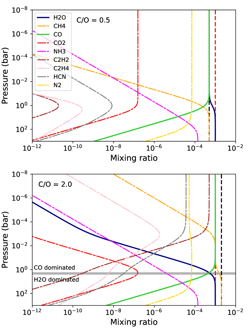
Figure 1: Thermochemical-equilibrium abundances for atmospheres with ${N_{\rm C}}/{N_{\rm O}}<1$ (top panel) and ${N_{\rm C}}/{N_{\rm O}}>1$ (bottom panel). Both atmospheres have a fixed temperature of 1200 K, ${N_{\rm O}}=5\times 10^{-4}$, and ${N_{\rm N}}=7\times 10^{-5}$. The black and red dashed vertical lines denote $2{N_{\rm C}}$ and $2{N_{\rm O}}$, which are related to the maximum values that carbon- and oxygen-bearing species can take, respectively. The gray horizontal line in the bottom panel denotes the turn-over pressure that separates CO- (above) and H₂O-dominated (below) regimes.

Therefore, we consider two main regimes: carbon- and oxygen-dominated atmospheres (${N_{\rm C}}\geq{N_{\rm O}}$ and ${N_{\rm O}}>{N_{\rm C}}$, respectively). Oxygen-dominated atmospheres are simple to deal with; since there is less carbon than oxygen available, ${N_{{{\rm CO}}}}$ cannot reach values equal to $f{N_{\rm O}}$ (Figure 1, top panel). Therefore, we always adopt Eq. (17), and solve the polynomial roots for CO.

Carbon-dominated atmospheres are more complex to deal with. Here, depending on the atmospheric properties, either ${N_{{{\rm H}_{2}{\rm O}}}}$ or ${N_{{{\rm CO}}}}$ can reach values close to $f{N_{\rm O}}$. Fortunately, H₂O and CO follow well-defined trends that allow us to estimate when either of them dominates the oxygen chemistry. In general, for a known temperature and set of elemental abundances, we can find a turn-over pressure ($p_{\rm to}$) above which CO dominates, and below which H₂O dominates (Figure 1, bottom panel). To map how $p_{\rm to}$ varies across our domain, we computed thermochemical-equilibrium abundances over a four-dimensional grid of temperatures and C, N, and O elemental abundances, using the open-source TEA package (Blecic et al., 2016). For each model, we then found the pressure where CO and H₂O switch places as the dominant species. For our application, we model $p_{\rm to}$ as a fourth-order polynomial in each of the four parameters, which matched the TEA $p_{\rm to}$ values at better than 20% at $T<3000$ K. This accuracy is sufficient for our purposes, since the range where an atmosphere transitions between H₂O and CO is typically wider. Then, whenever we wish to compute the analytic abundances, we compare the given pressure with $p_{\rm to}$ to determine whether we solve the polynomial roots for H₂O (CO-dominated atmospheres) or for CO (H₂O-dominated atmospheres).

For the same reason, we avoid using Equation (22) to obtain ${N_{{{\rm HCN}}}}$, but rather combine Equations (5) and (6) into Eq. (8) to find a quadratic polynomial for ${N_{{{\rm NH}_{3}}}}$:

$$2K_{5}\ ({N_{{{\rm NH}_{3}}}})^{2}+(1+K_{6}{N_{{{\rm CH}_{4}}}}){N_{{{\rm NH}_{3}}}}-f{N_{\rm N}}=0.$$ (26)

Only one of those roots is positive; thus, selecting the right solution is trivial. Then we use Eq. (23) to obtain the abundance of HCN.

4.3 Proper Approximations

Although in Section 4.2 we developed a strategy to avoid numerically unstable solutions, the root-finding algorithm may still fail to return physically plausible abundances. To ameliorate this issue, we tested several approximations that lower the degree of the polynomials, and hence, produce more robust results. The challenge is, given an atmosphere with an arbitrary temperature profile and elemental abundances, determining under which regimes we can neglect terms in Equations (16)–(25) without breaking the physics self consistency.

Initially, we considered three cases: neglecting all three nitrogen-bearing species, producing sixth-order polynomials (which we call the HCO solution); neglecting CO₂, C₂H₂, and C₂H₄, producing sixth-order polynomials; and neglecting only CO₂, producing eighth-order polynomials (HCNO solution). After testing, we discarded the second option since it was the least numerically reliable, and we found the other two approximations to be sufficient to cover the parameter space. Therefore, we proceed with the sixth-order HCO and eighth-order HCNO polynomials.

In general, the simpler HCO polynomials produce more stable solutions that are also faster to evaluate, making it our default choice. Equations (7) and (9) help us to determine when the HCO solution is appropriate (i.e., neglect the nitrogen-bearing species). Since the only link to nitrogen-bearing species relies on HCN, when $N_{{{\rm HCN}}}$ is negligible, the carbon and oxygen chemistry becomes virtually decoupled from the nitrogen chemistry. In this case, we can solve the system of equations considering only the HCO chemistry, without losing consistency for the entire system.

Overall, $N_{{{\rm HCN}}}$ decreases with decreasing temperature, with increasing pressure, or with decreasing $N_{{{\rm CO}}}$/$N_{{{\rm H}_{2}{\rm O}}}$. Therefore, we set threshold values in $T$ and ${N_{\rm N}}/{N_{\rm C}}$ to chose between the HCO or the HCNO approach. Similarly, we set threshold values in ${N_{\rm C}}/{N_{\rm O}}$ and use ${p_{\rm to}}$ to chose solving the polynomials for H₂O or CO. We use this theoretical insight to empirically find the threshold boundaries by evaluating all of our solutions over the parameter space. Figure 2 shows which polynomial approximation and variable we adopt for each case.

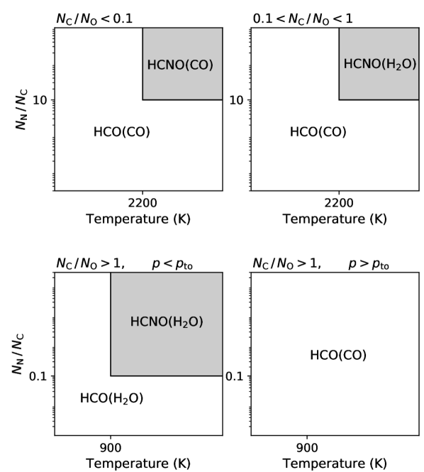
Figure 2: Schematic diagram of the solutions adopted for each case. In general, we adopt the HCNO polynomial at high temperatures and large ${N_{\rm N}}/{N_{\rm C}}$ ratio, because we need to consider the nitrogen chemistry; otherwise, we adopt the HCO polynomial. For ${N_{\rm C}}/{N_{\rm O}}<1$, we generally solve for the CO molecule because it never dominates the oxygen chemistry; whereas for ${N_{\rm C}}/{N_{\rm O}}>1$, we use ${p_{\rm to}}$ to chose the not-dominating molecule between CO or H₂O.

For ${N_{\rm C}}/{N_{\rm O}}<1$ atmospheres, we find the best results by applying the HCNO solution when ${N_{\rm N}}/{N_{\rm C}}>10$ and $T>2200$ K, for all other cases we apply the HCO solution. As expected, solving for CO produced more stable results, except for the HCNO case when $0.1<{N_{\rm C}}/{N_{\rm O}}<1$, where we solve for H₂O instead.

For ${N_{\rm C}}/{N_{\rm O}}\geq 1$ atmospheres, we find the best results by applying the HCNO solution when ${N_{\rm N}}/{N_{\rm C}}>0.1$ and $T>900$ K, but only when $p<{p_{\rm to}}$; for all other cases, we apply the HCO solution. We use $p_{\rm to}$ to decide to solve for the H₂O (CO-dominated atmosphere) or CO polynomial (H₂O-dominated).

5 Implementation and Benchmarking

We implemented the analytic framework described in this article into the rate open-source Python package, available at https://github.com/pcubillos/rate, which is compatible with Python 2.7 and 3. The routine takes typically 5–10 ms to evaluate a 100-layer atmosphere on a 3.60 GHz Intel Core i7-4790 CPU. We benchmarked the analytic abundances by comparing their results against the TEA code, computed under identical condition (i.e., same temperature, pressure, elemental composition, and output species).

We focus this exploration on the range of atmospheric properties probed by optical-to-infrared observations of sub-stellar objects. Thus, we select a pressure range from 100 to $10^{-8}$ bar; a temperature range from 200 to 6000 K; and metallicities from $10^{-3}$ to $10^{3}$ times solar values. Theoretical and observational studies argue that sub-stellar objects may have C/O ratios ranging from 0.1 to somewhat larger than unity (the solar C/O ratio is 0.55), depending on the formation scenario and evolution (see, e.g., Madhusudhan, 2012; Moses et al., 2013). Therefore, we further explore C/O ratios from 0.1 to 5.0.

Figures 3–8 show the accuracy of rate for each species. For each panel, we compute the metal elemental abundances such that they obey the labeled metallicity:

$${\rm[M/H]}=\log\frac{({N_{\rm C}}+{N_{\rm N}}+{N_{\rm O}})\phantom{{}_{\odot}}}{({N_{\rm C}}+{N_{\rm N}}+{N_{\rm O}})_{\odot}},$$ (27)

combined with the labeled elemental ratio for C/O = ${N_{\rm C}}/{N_{\rm N}}$, while maintaining a fixed solar elemental ratio for C/N = $({N_{\rm C}}/{N_{\rm N}})_{\odot}\approx 4$.

In general, we find a good agreement between rate and TEA, with no major variations in the accuracy as a function of C/O ratios. The accuracy of rate roughly correlates with the species abundances, meaning that the code performs better for the species that are more relevant for spectroscopy, particularly for the main species that determine the infrared spectrum of sub-stellar objects (e.g., H₂O, CO, and CH₄). For the relatively abundant species (mixing fractions larger than $10^{-10}$), the typical accuracy is better than 10%; for the less abundant species, the typical accuracy is better than 50%. The accuracy for each species varies differently with temperature, pressure, and metallicity, and is largely proportionally to the species abundance.

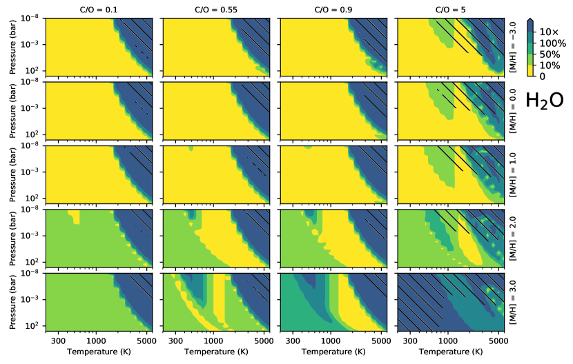
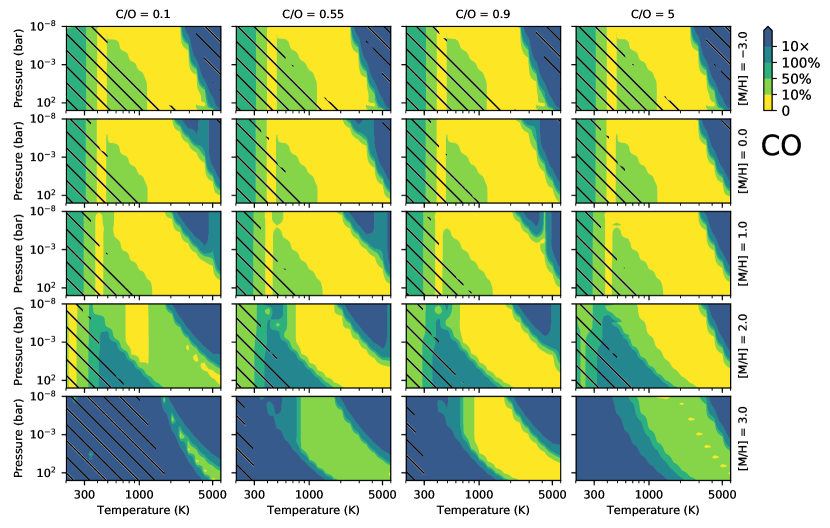
Figure 3: Difference between TEA and rate abundances for H₂O (top panels) and CO (bottom panels) coded by color (see top-right color bar). Each panels shows the TEA–rate difference in percentage as a function of temperature and pressure. For each species, the columns and rows show different values of C/O ratios and metallicities (see labels at the top and right side of the panels). Note the non-linear scale in metallicity (there are little differences for any sub-solar metallicity run). The hatched areas denote the regions where the species abundance drops below a mixing fraction of $10^{-10}$.

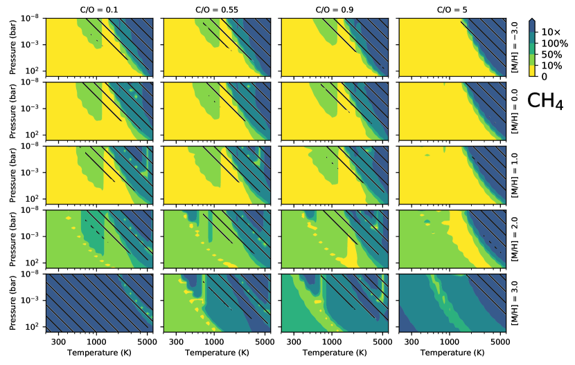
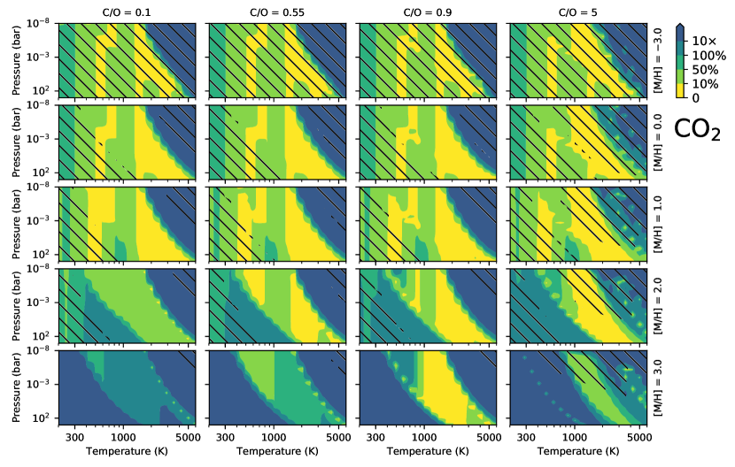
Figure 4: Difference between TEA and rate abundances for CH₄ (top panels) and CO₂ (bottom panels). See description in caption of Fig. 3.

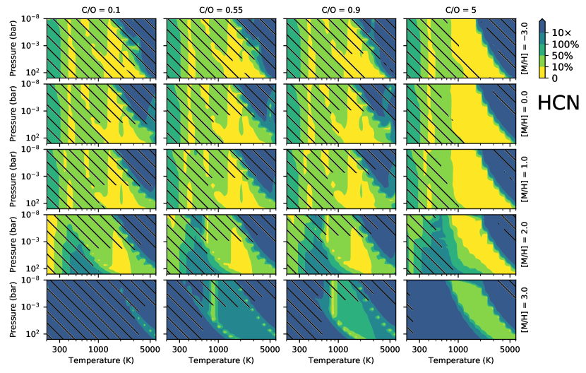
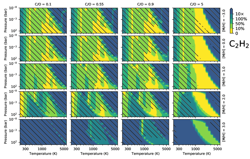
Figure 5: Difference between TEA and rate abundances for HCN (top panels) and C₂H₂ (bottom panels). See description in caption of Fig. 3.

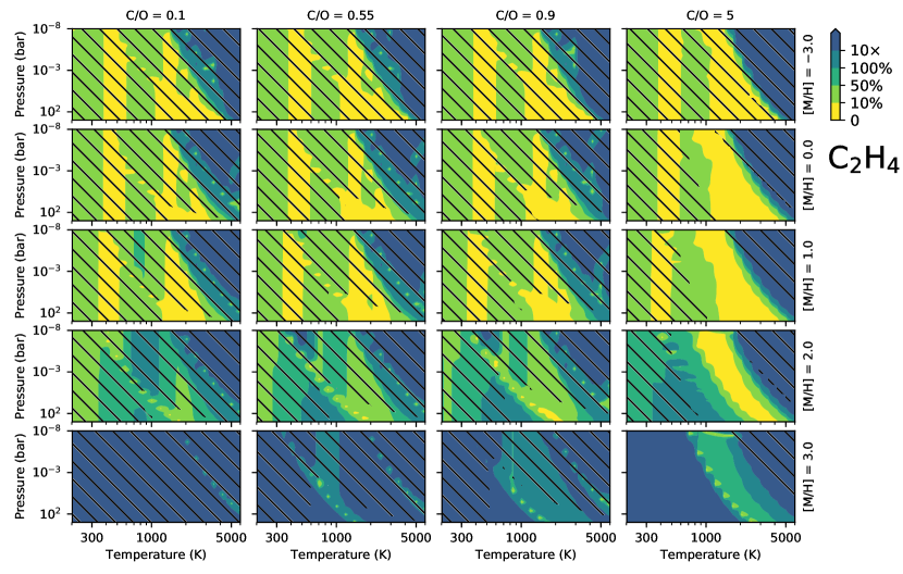
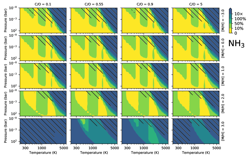
Figure 6: Difference between TEA and rate abundances for C₂H₄ (top panels) and NH₃ (bottom panels). See description in caption of Fig. 3.

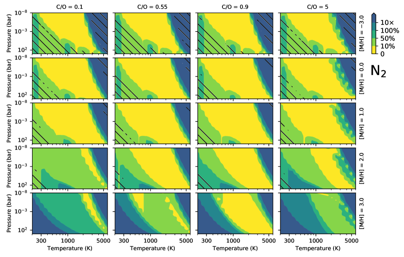
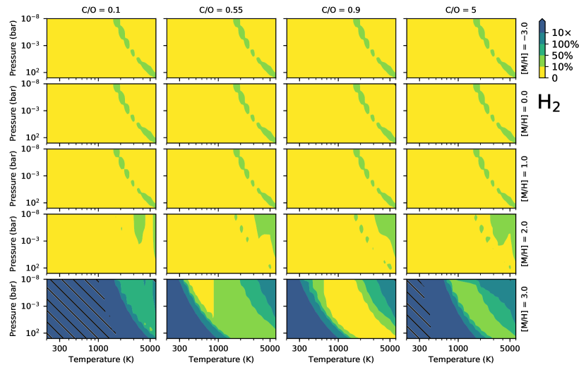
Figure 7: Difference between TEA and rate abundances for N₂ (top panels) and H₂ (bottom panels). See description in caption of Fig. 3.

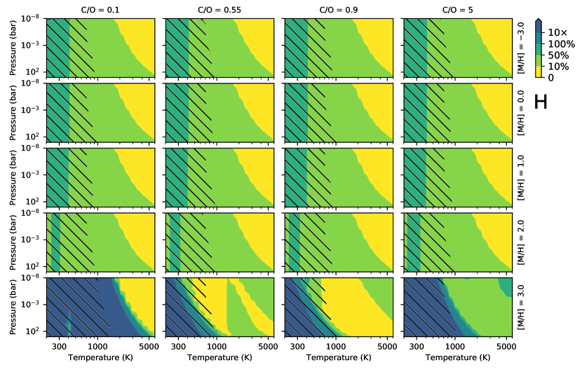
Figure 8: Difference between TEA and rate abundances for H. See description in caption of Fig. 3.

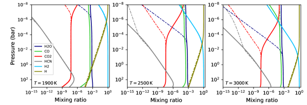
Figure 9: Comparison between analytic (solid curves) and TEA (dashed curves) thermochemical-equilibrium abundances, at increasing temperatures (left, middle, and right panels). Only a selected subset of species id shown (see legend). The atmosphere has a nearly solar composition with ${N_{\rm C}}=1.5\times 10^{-4}$, ${N_{\rm O}}=5.0\times 10^{-4}$, and ${N_{\rm N}}=7.0\times 10^{-5}$. As the temperature increases, the analytic values deviate from the thermochemical-equilibrium values at progressively lower pressures, due to the dissociation of the molecular species.

We find two distinctive regions where rate does not perform well. There is a sharp decrease in accuracy at a combination of high temperatures and low pressures. Starting at $T\gtrsim 2000$ K at the $\sim$bar level, the boundary of this region propagates toward higher pressures as the temperature increases (see top-right corner of panels in Figs. 3–8). In this case, the molecules start to dissociate into their atomic form, which we do not account for metals (i.e., C, N, and O). In particular, the analytic approach overestimates the abundances for H₂O and CO₂, compared to their expected thermochemical-equilibrium values (Figure 9). We emphasize that this is not an implementation issue, the outputs reflect exactly what the equations indicate. Rather, the analytic approach fails to fully trace the physics of the problem. Similarly, the accuracy starts to decrease proportionally with the increasing metallicity for super solar values. From 100 to 1000 times solar metallicity, rate produces abundances deviating by a factor of 2 to more than 10 times from the expected values, respectively. In this case, the assumption of hydrogen-dominated atmosphere is no longer valid, and the analytic results become inaccurate.

6 Conclusions

We have developed a framework that expands on the work of Heng et al. (2016), Heng & Lyons (2016), and Heng & Tsai (2016), to analytically compute thermochemical-equilibrium abundances for a chemical system with arbitrary temperature, pressure, and elemental abundances. This approach computes the mole mixing ratios for H₂O, CH₄, CO, CO₂, NH₃, C₂H₂, C₂H₄, HCN, N₂, H₂, atomic H, and He, by finding the roots of a univariate polynomial expression. We implemented this approach into the rate open-source package (compatible with Python 2.7 and 3), which is available at https://github.com/pcubillos/rate.

To obtain the analytic equations, we developed a general and nearly effortless approach to find the polynomial coefficients using sympy, which facilitates future development of this approach. In our system of equations, we accounted for atomic hydrogen (in addition to molecular hydrogen), which is the dominant hydrogen-bearing molecule at high temperatures and low pressures, due to dissociation. We treat He as a constant-abundance non-interacting species.

We found three key factors that improve the numerical stability of the analytic approach over prior efforts: we apply a more reliable algorithm to solve for the polynomial roots; we identify and avoid the regimes where solving polynomials for H₂O or CO is numerically unstable; and we identify the regimes where one can neglect HCN, and thus decouple the nitrogen chemistry from the carbon and oxygen equations to find simpler polynomial expressions.

This code computes reliable abundances over a range of pressures from $10^{-8}$ to $10^{3}$ bar; temperatures from 200 to $\sim$2000 K; and elemental metallicities from $10^{-3}$ to $\sim\!10^{2}\times$ solar values. Beyond these boundaries, the assumptions of this framework do not apply anymore, and thus, the the analytic solutions become less accurate, i.e., molecules dissociate into atoms at higher temperatures, and the composition is no longer hydrogen-dominated at higher metallicities.

Our framework produces abundances with an accuracy better than 10% of their expected values for the more abundant species (mixing ratios larger than $10^{-10}$), and therefore, those more relevant for spectroscopy. Ultimately, different applications will have different accuracy requirements. For example, for exoplanet atmospheric characterization, we do not expect to find abundance uncertainties much better than 50% for the dominant species (Greene et al., 2016). Our improvements enable us to use the fast analytic approach to compute reliable equilibrium abundances over a wide range of temperatures, pressures, and elemental abundances. With the exception of the extreme ultra-hot Jupiters, this framework is of particular interest to model and retrieve the observed atmosphere of most giant-exoplanet atmospheres, since the molecules considered here are the main species that dominate the infrared and optical spectrum of these planets.

The Reproducible Research Compendium of this article is available at 10.5281/zenodo.2529532 (catalog 10.5281/zenodo.2529532).

References

- AAS Journals Team & Hendrickson (2018) AAS Journals Team, & Hendrickson, A. 2018, Aasjournals/Aastex60: Version 6.2 Official Release, ADS
- Allard & Hauschildt (1995) Allard, F., & Hauschildt, P. H. 1995, ApJ, 445, 433, ADS, astro-ph/9601150
- Allard et al. (1996) Allard, F., Hauschildt, P. H., Baraffe, I., & Chabrier, G. 1996, ApJ, 465, L123, ADS
- Blecic et al. (2016) Blecic, J., Harrington, J., & Bowman, M. O. 2016, ApJS, 225, 4, ADS, 1505.06392
- Burrows & Sharp (1999) Burrows, A., & Sharp, C. M. 1999, ApJ, 512, 843, ADS, astro-ph/9807055
- Chase (1986) Chase, M. W. 1986, JANAF thermochemical tables, ADS
- Cubillos (2019) Cubillos, P. E. 2019, bibmanager: A BibTeX manager for LaTeX projects
- Fegley & Lodders (1996) Fegley, Jr., B., & Lodders, K. 1996, ApJ, 472, L37, ADS
- Greene et al. (2016) Greene, T. P., Line, M. R., Montero, C., Fortney, J. J., Lustig-Yaeger, J., & Luther, K. 2016, ApJ, 817, 17, ADS, 1511.05528
- Heng & Lyons (2016) Heng, K., & Lyons, J. R. 2016, ApJ, 817, 149, ADS, 1507.01944
- Heng et al. (2016) Heng, K., Lyons, J. R., & Tsai, S.-M. 2016, ApJ, 816, 96, ADS, 1506.05501
- Heng & Tsai (2016) Heng, K., & Tsai, S.-M. 2016, ApJ, 829, 104, ADS, 1603.05418
- Hunter (2007) Hunter, J. D. 2007, Computing in Science and Engineering, 9, 90, ADS
- Jones et al. (2001) Jones, E., Oliphant, T., Peterson, P., et al. 2001, SciPy: Open source scientific tools for Python
- Lodders & Fegley (2002) Lodders, K., & Fegley, B. 2002, Icarus, 155, 393, ADS
- Madhusudhan (2012) Madhusudhan, N. 2012, ApJ, 758, 36, ADS, 1209.2412
- Marley & Robinson (2015) Marley, M. S., & Robinson, T. D. 2015, ARA&A, 53, 279, ADS, 1410.6512
- Meurer et al. (2017) Meurer, A. et al. 2017, PeerJ Computer Science, 3, e103
- Moses et al. (2013) Moses, J. I. et al. 2013, ApJ, 777, 34, ADS, 1306.5178
- Moses et al. (2011) Moses, J. I. et al. 2011, ApJ, 737, 15, ADS, 1102.0063
- Perez & Granger (2007) Perez, F., & Granger, B. E. 2007, Computing in Science and Engineering, 9, 21, ADS
- Press et al. (2002) Press, W. H., Teukolsky, S. A., Vetterling, W. T., & Flannery, B. P. 2002, Numerical recipes in C++ : the art of scientific computing, ADS
- Tsai et al. (2017) Tsai, S.-M., Lyons, J. R., Grosheintz, L., Rimmer, P. B., Kitzmann, D., & Heng, K. 2017, ApJS, 228, 20, ADS, 1607.00409
- Tsuji (1973) Tsuji, T. 1973, A&A, 23, 411, ADS
- Tsuji et al. (1996) Tsuji, T., Ohnaka, K., Aoki, W., & Nakajima, T. 1996, A&A, 308, L29, ADS
- van der Walt et al. (2011) van der Walt, S., Colbert, S. C., & Varoquaux, G. 2011, Computing in Science and Engineering, 13, 22, ADS, 1102.1523
- Visscher et al. (2006) Visscher, C., Lodders, K., & Fegley, Jr., B. 2006, ApJ, 648, 1181, ADS, arXiv:astro-ph/0511136
- Visscher et al. (2010a) Visscher, C., Lodders, K., & Fegley, Jr., B. 2010a, ApJ, 716, 1060, ADS, 1001.3639
- Visscher et al. (2010b) Visscher, C., Moses, J. I., & Saslow, S. A. 2010b, Icarus, 209, 602, ADS, 1003.6077
- Zahnle et al. (2009) Zahnle, K., Marley, M. S., Freedman, R. S., Lodders, K., & Fortney, J. J. 2009, ApJ, 701, L20, ADS, 0903.1663
- Zolotov & Fegley (1998) Zolotov, M. Y., & Fegley, B. 1998, Icarus, 132, 431, ADS