Torus knot choreographies in the $n$-body problem

Abstract

We develop a systematic approach for proving the existence of choreographic solutions in the gravitational $n$ body problem. Our main focus is on spatial torus knots: that is, periodic motions where the positions of all $n$ bodies follow a single closed which winds around a $2$-torus in $\mathbb{R}^{3}$. After changing to rotating coordinates and exploiting symmetries, the equation of a choreographic configuration is reduced to a delay differential equation (DDE) describing the position and velocity of a single body. We study periodic solutions of this DDE in a Banach space of rapidly decaying Fourier coefficients. Imposing appropriate constraint equations lets us isolate choreographies having prescribed symmetries and topological properties. Our argument is constructive and makes extensive use of the digital computer. We provide all the necessary analytic estimates as well as a working implementation for any number of bodies. We illustrate the utility of the approach by proving the existence of some spatial choreographies for $n=4,5,7$, and $9$ bodies.

1 Introduction

A choreography is a periodic solution of the gravitational $n$-body problem, where $n$ equal masses follow the same path. Circular choreographies with masses located at the vertices of a regular $n$-gon were already studied by Lagrange in the Eighteenth Century. The first choreography differing from a polygon was discovered by Moore in [1] and has three bodies moving around the now famous figure-eight. Chenciner and Montgomery in [2] gave a rigorous mathematical proof of the existence of this figure eight orbit by minimizing the action for Newton’s equation. The name choreographies was adopted after the work of Simó [3] on numerical computation of choreographic solutions.

The variational approach to the existence of choreographies consists of finding critical points of the classical Newtonian action subject to appropriate symmetry constraints. The main obstacle to this approach is the existence of paths with collisions. Terracini and Ferrario in [4] gave conditions on the symmetries which imply that a minimizer is free of collisions (this is called the rotating circle property). Although a lot of simple choreographies have been found numerically since Simó [3], rigorous proofs using only analytical methods are difficult. Notable exceptions include works on: the figure-eight of three bodies [2], the rotating $n$-gon [5], the figure-eight type for odd bodies [4] and the super-eight of four bodies [6]. Other variational approaches related to existence of planar choreographies can be found in [7, 8, 9, 10, 11, 12] and the references therein.

The difficulties just mentioned have led some authors to develop mathematically rigorous computer assisted proofs (CAPs) for choreographies. This is a natural alternative to pen-and-paper analysis since both the discovery and many subsequent studies of choreographies employ numerical methods. The interested reader will want to consult for example the works of Kapela, Simó, and Zgliczyński [13, 14, 15] for both CAPs of existence for planar choreographies and mathematically rigorous stability analysis. See also Remark 2 below.

Recall now that a $(p,q)$-torus knot is an embedding of $\mathbb{S}^{1}$ into a two torus $\mathbb{T}^{2}\subset\mathbb{R}^{3}$, winding $p$ times around one generating circle of the torus and $q$ times around the other, with $p$ and $q$ coprime and neither equal to zero. The embedding of the two torus is required to be unknotted in $\mathbb{R}^{3}$. A torus knot may or may not be a trivial when viewed as a knot in $\mathbb{R}^{3}$. Indeed, it is trivial if and only if either $p$ or $q$ is equal to $\pm 1$. The idea is illustrated in Figure 1.

Figure 1: Spatial torus knots: given an unknotted $2$-torus embedded in $\mathbb{R}^{3}$, a $(p,q)$-torus knot is a non-contractible curve embedded into the surface of the torus. The curve then winds $p$ and $q$ times respectively around the generating circles of the torus (with $p$ and $q$ co-prime). It is a basic result that a $(p,q)$ torus knot is trivial as a knot in $\mathbb{R}^{n}$ if and only if either $p$ or $q$ is $\pm 1$. The left frame illustrates a torus knot which is a trivial knot in $\mathbb{R}^{3}$, while the right frame illustrates a non-trivial $(3,2)$-knot – in fact a trefoil.

A difficult problem in this area is to prove the existence of spatial torus knot choreographies. Indeed when both topological and symmetric constraints are involved, it is difficult to prove the coercitivity of the action. For this reason few results with topological constraints are available. A notable exception is a torus knot choreography for $3$-bodies obtained by Arioli, Barutello, and Terracini in [16], where the authors localize a mountain pass solution of the Newtonian action in a rotating frame. Again the result is obtained by means of CAP, not variational methods. In general it is hard to determine whether a critical point of the action is a spatial torus-knot choreography. We provide a systematic procedure to obtain countable families of torus knots for any number of bodies.

Contribution: The main result of the present work is to give mathematically rigorous existence proofs for $(p,q)$-torus knot choreographies in the $n$-body problem for several different values of $n$.

Our approach is functional analytic (a choreography is a zero of a nonlinear operator posed on a Banach space) and computer-assisted. When it succeeds it produces countably many verified results. For example we establish the existence of the $5$-body trefoil knot choreography illustrated in Figure 2, and the existence of countable many choreographies close to it. We describe the pen and paper estimates for any number of bodies and, while we illustrate the method for only few explicit examples, our setup and resulting implementation apply (in principle) to any spatial choreography.

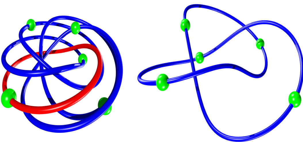
Figure 2: Example of a spatial trefoil choreography for 5 bodies: Left frame (rotating coordinates) the red loop illustrates the periodic orbit of the delay differential equation whose existence we prove using the methods of the present work. The four remaining loops are obtained by symmetry, giving a periodic orbit of the full 5 body problem in rotating coordinates. Right frame (inertial coordinates) the 5 body orbit converted to rotating coordinates. The result is a spatial torus knot with the topology of a trefoil.

Before describing our approach in detail we recall several related developments. In [17] it is observed that choreographies appear in dense sets along the vertical Lyapunov families attached to the relative equilibrium solutions given by the planar $n$-gon . Existence of vertical Lyapunov families follows from the Weinstein-Moser theory and, when the frequency varies continuously, the authors obtain the existence of an infinite number of choreographies along these vertical families. This hypothesis however has been verified only for some families with $n=3,4,5,6$ and even though similar computations can be carried out for other values of $n$, it is an open problem to establish the hypothesis for all $n$.

The existence of global Lyapunov families arising from the polygonal relative equilibrium of the rotating problem was established in [18, 19] for all $n$. By saying that these families are global what we mean that, in the space of normalized $2\pi$ periodic solutions, the families form a continuum set with at least one of the following properties: either the Sobolev norm of the orbits in the family goes to infinity, the period of the orbits goes to infinity, the family ends in an orbit with collision, or the family returns to another equilibrium solution. This fact is proved using $G$-equivariant degree theory [20] where $G=\mathbb{Z}_{n}\times\mathbb{Z}_{2}\times SO(2)\times S^{1}$ acts as permutations, $z$-reflection and $(x,y)$-rotations of bodies, and time shift respectively. In addition the analysis of [18, 19] concludes that the Lyapunov families have the symmetries of a twisted subgroup of $G$.

Specifically, let $(w_{j},z_{j})\in\mathbb{C}\times\mathbb{R}$ represents the planar and spatial coordinates of the $j$-th body in a rotating coordinate frame with frequency $\sqrt{s_{1}}$, where

$$s_{1}=\frac{1}{4}\sum_{j=1}^{n-1}\frac{1}{\sin(j\zeta/2)},\qquad\zeta=\frac{2\pi}{n}.$$ (1)

The $n$-polygon consisting of $n$ bodies on the unit circle $w_{j}=e^{ij\zeta}$ is an equilibrium solution of Newton’s equations in a co-rotating frame. After normalizing the period to $2\pi$, the planar Lyapunov families arising from this equilibrium polygon have the planar symmetries,

$$w_{j}(t)=e^{ij\zeta}w_{n}(t+jk\zeta),$$ (2)

and the spatial symmetries

$$z_{j}(t)=z_{n}(t+jk\zeta).$$ (3)

For $1\leq j\leq n-1$ the $j$-th body follows an identical path as the $n$-th body, after a rotation in space and a shift in time. It is proved in [19] that taking $k=2,..,n-2$ in the planar case gives the $n-3$ planar Lyapunov families, and that taking $k=1,...,n-1$ in the spatial case gives the $n-1$ vertical Lyapunov families.

We stress that the $G$-equivariant degree theory provides only an alternative concerning the global behavior of the Lyapunov families. Without additional information we do not know what actually happens along a given branch. This question is considered in [21], where the authors conduct a numerical exploration of the global behavior of the Lyapunov families using the software package AUTO (e.g. see [22]).

Let $p,q\in\mathbb{Z}$ be relatively prime such that $kq-p\in n\mathbb{Z}$. It is proved in [21] that an orbit with the symmetries defined in equations (2) and (3), and frequency

$$\omega=\sqrt{s_{1}}\frac{p}{q},$$ (4)

is a simple choreography when converted back to the inertial reference frame. In the case that $p$ and $q$ do not satisfy this diophantine equation, the solution in the inertial frame corresponds to a multiple choreographic solution [8], while the case that $\omega/\sqrt{s_{1}}$ is irrational implies that the solution is quasiperiodic. Since the set of rational numbers $p/q$ satisfying the diophantine relation (4) is dense, one has the following: when the frequency $\omega$ varies continuously along the Lyapunov family, there are infinitely many orbits in the rotating frame that correspond to simple choreographies in the inertial frame.

The authors of [21] give compelling numerical evidence which suggests that an axial family of solutions appears after a symmetry-breaking bifurcation from the vertical Lyapunov family in the rotating $n$-body problem. The numerics suggest that this axial family has the symmetries of equations (2) and (3). It is shown further in the same reference that, if the hypothesized axial family exists, then orbits in this family correspond to choreographies in the inertial frame which wind $p$ and $q$ times around the generators of a $2$-torus. That is, the periodic orbits in this alleged axial family give rise to $(p,q)$-torus knot choreographies for the $n$-body problem.

A more refined description of our contribution is that we prove the existence of this axial family. Using the symmetries (2, 3) in Newton’s laws we reduced the equations of motion to a single equation describing the motion of the $n$-th body $u_{n}=(w,z)\in\mathbb{C\times R}$. The equation is a delay differential equation (DDE) with multiple constant delays. More explicitly, we have

$$\begin{array}[c]{rl}\ddot{w}(t)+2\sqrt{s_{1}}i\dot{w}(t)&=\displaystyle s_{1}w(t)-\sum_{j=1}^{n-1}\frac{w(t)-e^{ij\zeta}w(t+jk\zeta)}{\left(\left|w(t)-e^{ij\zeta}w(t+jk\zeta)\right|^{2}+\left|z(t)-z(t+jk\zeta)\right|^{2}\right)^{3/2}}\\ \ddot{z}(t)&=\displaystyle-\sum_{j=1}^{n-1}\frac{z(t)-z(t+jk\zeta)}{\left(\left|w(t)-e^{ij\zeta}w(t+jk\zeta)\right|^{2}+\left|z(t)-z(t+jk\zeta)\right|^{2}\right)^{3/2}}.\end{array}$$ (5)

For any number of bodies, these reduced equations (5) represents a system of six scalar equations with multiple constant delays.

Our computer assisted arguments are in the functional analytic tradition of Lanford, Eckamnn, Koch, and Wittwer [23, 24, 25, 26], and build heavily on the earlier work of [27, 28, 29] on DDEs. More precisely, we formulate the existence proofs on a Banach space of Fourier coefficient sequences. The delay operator acts as a multiplicative (diagonal) operator in Fourier coefficient space, and the regularity of periodic solutions translates into rapid decay of the Fourier coefficients. Indeed, as was shown in [30], a periodic solution of a delay differential equation with analytic nonlinearity is analytic when the delays are constant. Then we know a-priori that the Fourier coefficients of a periodic solution of Equations (5) decay exponentially fast.

An important feature of Equations (5) is the conservation of energy, which allows us to fix a desired frequency for the periodic solution a-priori. This reduction greatly simplifies the analysis of the delay differential equation in Fourier space, but requires adding an unfolding parameter to balance the system. In addition we utilize automatic differentiation as in [31, 32, 33], and reformulate (5) as a problem with polynomial nonlinearities. The polynomial problem is amenable to straight forward analysis exploiting the Banach algebra properties of the solution space and we use the FFT algorithm as in [34]. The cost of this simplification is that each additional body augments the system with a single additional scalar equation and a single additional unfolding parameter. Finally we validate the existence of solutions by means of a Newton-Kantorovich argument exploiting the radii polynomial approach as in [35].

We conclude this introduction by mentioning some interesting problems for future study. The zero finding problem studied in the present work is amenable to validated continuation techniques as discussed in [29, 36, 37, 38]. A follow up study will investigate global properties of continuous families of spatial choreographies in the $n$ body problem, and study bifurcations encountered along the branches. In this way we hope to prove for example the conjecture of Marchal/Chenciner [17] that the Lagrange triangle is connected with the figure-eigth choreography trough Marchal’s P-12 family [39]. We also remark that all the choreographies shown to exist in the present work are unstable. Actually, the only known stable choreographies are close to the figure eight for $n=3$. Stability of torus knots in the $n=3$ is being investigated in a forthcoming paper.

Let us also mention that the procedure developed in this paper could be adapted to prove existence of asymmetric planar or spatial choreographies. These choreographies do appear in dense sets of symmetry-breaking families from planar and spatial Lyapunov families. Furthermore, this procedure could be adapted to study choreography solutions in problems with other potentials, such as $r^{-\alpha}$ (with $\alpha=1$ being the gravitational case, $\alpha<1$ the weak force case, and $\alpha>2$ the strong force case). It could also be adapted to Hamiltonian systems with different radial potentials, as long as the polynomial embedding (see Section 2.3) can be done. An interesting problem would be to adapt the method to validate choreographies in families that bifurcate from the polygonal equilibrium in DNLS equations [40] or the $n$-vortex problem on the plane, disk, or sphere [41].

Remark 1 (CAPs in celestial mechanics and dynamics of DDEs).

Numerical calculations have been central to the development of celestial mechanics since the late Nineteenth and early Twentieth centuries. The reader interested in historical developments before the age of the digital computer can consult the works of George Darwin, Francis Ray Moulton, and the group in Copenhagen led by Elis Strömgren [42, 43, 44]. Problems in celestial navigation and orbit design helped drive the explosion of scientific computing during the space race of the mid Twentieth century. A fascinating account and a much more complete bibliography are found in the book [45].

As researchers developed computer assisted methods of proof for computational dynamics it was natural to look for challenging open problems in celestial mechanics. The relevant literature is rich and we direct the interested reader to the works of [46, 47, 16, 48, 49] for a much more complete view of the literature. Other authors have studied center manifolds [50], transverse intersections of stable/unstable manifolds [31, 51], Melnikov theory [52], Arnold diffusion and transport [53, 54, 55], and existence/continuation/bifurcation of Halo orbits [32, 56] – all in gravitational $n$-body problems and all using computer assisted arguments. Especially relevant to the present work are the computer assisted existence and KAM stability proofs for $n$-body choreographies in [13, 14, 15, 16]. (See also Remark 2 below). Again, the references given in the preceding paragraph are meant only to point the reader in the direction of the relevant literature. A more complete view of the literature is found in the references of the cited works.

The present work grows out of the existing literature on CAPs for dynamics of DDEs, the foundations of which were laid in [27]. The work just cited studied periodic solutions – as well as branches of periodic solutions – for scalar DDEs with a single delay and polynomial nonlinearities. Extensions to multiple delays appear in [28], and more recent work considers systems of DDEs with non-polynomial nonlinearities [33]. The interested reader can consult the works of [29, 57, 58, 59] for more complete discussion of this area. We mention also the recent Ph.D. thesis of Jonathan Jaquette, who settled the decades old conjectures of Wright and Jones about the global dynamics of Wright’s equation [60, 61] using ideas from this field. Another approach to computer assisted proof for periodic orbits of DDEs – based on rigorous integration of the induced flow in function space – is found in [62].

In spite of the picture painted above, computer assisted methods of proof are regularly applied outside the boundaries of celestial mechanics and delay differential equations. For a broader perspective on the area, still focusing on nonlinear dynamics, we refer to the review articles [63, 64] and to the book of Tucker [65].

Remark 2 (Phase space and functional analytic approaches).

The existence proofs for planar choreographies in [13] and [15], the proof of the spatial mountain pass solution in [16], and the proof of KAM stability of the figure eight choreography in [14] use a different setup from that developed in the present work. More precisely, the works just mentioned study directly the Newtonian equations of motion in phase space. The works of [13, 15, 14] exploit the powerful CAPD library for rigorous integration of ODEs to construct mathematically rigorous arguments in appropriate Poincaré sections. See [66, 67] for more complete discussion and references to the CAPD library. The work of [16] utilizes a functional analytic method akin to that of the present work, but applied directly to periodic orbits for the Hamiltonian vector field rather than reducing to the delay differential equation as in the present work.

In the case of the planar choreography problem the phase space is of dimension $4n$, while the spatial choreography problem scales like $6n$. These figures are in some sense conservative, as applying the topological arguments of [13, 15] require integration of the equations of first variation (and equations of higher variation in the case of the KAM stability argument).

The setup of the present work considers six scalar equations, independent of the number of bodies considered. This is a dramatic reduction of the dimension of the problem. This dimension reduction facilitates consideration of – in principle – choreographies involving any number of bodies. A technical remark is that our implementation uses automatic differentiation to reduce to a polynomial nonlinearity, adding one additional scalar equation for each body being considered. This brings our count to $6+(n-1)$ scalar equations. While this quantity scales with $n$ much better than the $6n$ mentioned above, we stress that our implementation could be improved using techniques similar to those discussed in [16, 68, 69] for evaluation of non-polynomial nonlinearities on Fourier data. With such an improvement our approach would consider only 6 scalar equations no matter the number of bodies.

For the sake of simplicity we do not pursue this option at the present time, as we believe that the reduction to a polynomial nonlinearity makes both the presentation and implementation of the method more transparent. We also believe that the polynomial version of the problem is more amenable to high order branch following methods and bifurcation analysis to be pursued in a future work. We remark that, since we work in a space of analytic functions, our argument produces useful by-products such as bounds on coefficient decay rates, and lower bounds on the domain of analyticity/bounds on the distances to poles in the complex plane. This information can be used to obtain a-posteriori bounds on derivatives via the usual Cauchy bounds of complex analysis.

The paper is organized as follows. In Section 2, we introduce the Fourier map $F:X\to Y$ defined on a Banach space $X$ of geometrically decaying Fourier coefficients, whose zeros are choreographies having prescribed symmetries and topological properties. In Section 3, we introduce the ideas of the a-posteriori validation for the Fourier map, that is on how to demonstrate the existence of true solutions of $F(x)=0$ close to numerical approximations. In Section 4, we present explicit formulas for the bounds necessary to apply the a-posteriori validation of Section 3. We conclude the paper by presenting the results in Section 5, where we present proofs of existence of some spatial torus knot choreographies for $n=4,5,7$, and $9$ bodies. The computer programs used in the paper are available at [70].

2 Formulation of the problem

Let $q_{j}(t)\in\mathbb{R}^{3}$ be the position in space of the body $j\in\{1,...,n\}$ with mass $1$ at this $t$. Define the matrices

$$\bar{I}=diag(1,1,0)\text{ and }\bar{J}=diag(J,0)\text{,}$$

where $J$ is the symplectic matrix in $\mathbb{R}^{2}$. In rotating coordinates and with the period rescaled to $2\pi$,

$$q_{j}(t)=e^{\sqrt{s_{1}}t\bar{J}}u_{j}(\omega t),$$

the Newton equations for the $n$ bodies are

$$\omega^{2}\ddot{u}_{j}+2\omega\sqrt{s_{1}}\bar{J}\dot{u}_{j}-s_{1}\bar{I}u_{j}=-\sum_{i=1(i\neq j)}^{n}\frac{u_{j}-u_{i}}{\left\|u_{j}-u_{i}\right\|^{3}},$$ (6)

where $\omega$ is the frequency and $s_{1}$ is defined by (1).

Using that $u_{j}=(w_{j},z_{j})$, the symmetries (2) and (3) correspond to the symmetry

$$u_{j}(t)=e^{\ j\bar{J}\zeta}u_{n}(t+jk\zeta)\text{.}$$ (7)

Therefore, the solutions of the equation (6) with symmetries (7) are zeros of the map

$$\mathcal{G}(u_{n},\omega)\,\stackrel{{\scriptstyle\mbox{\tiny{\raisebox{0.0pt}[0.0pt][0.0pt]{def}}}}}{{=}}\,\omega^{2}\ddot{u}_{n}+2\omega\sqrt{s_{1}}\bar{J}\dot{u}_{n}-s_{1}\bar{I}u_{n}+\sum_{j=1}^{n-1}\frac{u_{n}-e^{\ j\bar{J}\zeta}u_{n}(t+jk\zeta)}{\left\|u_{n}-e^{\ j\bar{J}\zeta}u_{n}(t+jk\zeta)\right\|^{3}}:X\times\mathbb{R}\rightarrow Y$$ (8)

defined in spaces $X$ and $Y$ of analytic $2\pi$-periodic functions, which we will specify later in Fourier components. The equation $\mathcal{G}(u_{n},\omega)=0$, with $\mathcal{G}$ defined in (8) is a delay differential equation (DDE).

2.1 Choreographies

We say that a solution of $\mathcal{G}(u_{n},\omega)=0$, i.e. a solution of the $n$-body problem with symmetry (7), is $p:q$ resonant when it has frequency $\omega=\sqrt{s_{1}}p/q$ and (a) $kq-p=0$ or (b) $p$ and $q$ are relatively prime and $kq-p\in n\mathbb{Z}$. In [21] is proven that $p:q$ resonant orbits are choreographies in the inertial frame, see also [17]. For sake of completeness, here we reproduce a short version of this result.

Proposition 3.

Let

$$Q_{j}(t)\,\stackrel{{\scriptstyle\mbox{\tiny{\raisebox{0.0pt}[0.0pt][0.0pt]{def}}}}}{{=}}\,q_{j}(t/\omega)=e^{t\bar{J}\sqrt{s_{1}}/\omega}u_{j}(t)$$

be a reparameterization of a periodic solution in the inertial frame. An $p:q$ resonant solution $u_{n}\$of $\mathcal{G}(u_{n},\omega)=0$ is a choreography in inertial frame, satisfying that $Q_{n}(t)$ is $2\pi p$-periodic and

$$Q_{j}(t)=Q_{n}(t+j\tilde{k}\zeta)\text{,}$$

where $\tilde{k}=k-(kq-p)\tilde{q}$ with $\tilde{q}$ the $p$-modular inverse of $q$. The orbit of the choreography is symmetric with respect to rotations by an angle $2\pi/p$ and the $n$ bodies form groups of $h$-polygons, where $h$ is the biggest common divisor of $n$ and $k$.

Proof.

Since $u_{n}(t)$ is $2\pi$-periodic and $e^{t\bar{J}\sqrt{s_{1}}/\omega}=e^{t\bar{J}q/p}$ is $2\pi p$-periodic, then the function $Q_{n}(t)=e^{t\bar{J}\sqrt{s_{1}}/\omega}u_{n}(t)$ is $2\pi p$-periodic. Furthermore, since

$$Q_{n}(t-2\pi)=e_{n}^{-\bar{J}2\pi q/p}Q_{n}(t),$$ (9)

the orbit of $Q_{n}(t)$ is invariant under rotations of $2\pi/p$. The fact that the $n$ bodies form $h$-polygons follows from symmetry (7) and the definition of $Q_{j}(t)$.

By assumption

$$r=(kq-p)/n\in\mathbb{Z},$$

then symmetry (7) implies that the solution in inertial frame satisfies

$$Q_{j}(t)=e^{-\bar{J}2\pi j(r/p)}Q_{n}(t+jk\zeta)\text{.}$$ (10)

In the case (a) that $kq-p=0$, the symmetry (9) gives straightforward that $Q_{j}(t)=Q_{n}(t+kj\zeta)$. In the case (b) that $p$ and $q$ are relatively prime, we can find $\tilde{q}$ such that $q\tilde{q}=1$ mod $p$. It follows from the symmetry (9) that

$$Q_{n}(t-2\pi jr\tilde{q})=e^{-\bar{J}2\pi j(r/p)}Q_{n}(t).$$

Therefore,

$$Q_{j}(t)=e^{-\bar{J}2\pi j(r/p)}Q_{n}(t+jk\zeta)=Q_{n}(t+j(k-rn\tilde{q})\zeta).\qed$$

Corollary 4 ($(p,q)$-torus knots).

In the case that $u_{n}(t)$ is a $p:q$ resonant orbit in the axial family that does not cross the $z$-axis, then $Q_{n}(t)$ winds (after the period $2\pi p$) around a toroidal manifold with winding numbers $p$ and $q$, i.e., the choreography path is a $(p,q)$-torus knot. In the case that $u_{n}(t)$ is a $p:q$ resonant orbit in the vertical Lyapunov family that does not cross the $z$-axis, then the choreography $Q_{n}(t)$ winds $p$ times in a cylindrical surface.

We conclude that the solution $q_{j}(t)=Q_{j}(t\omega)$ is a $2\pi q/\sqrt{s_{1}}$-periodic choreography satisfying the properties discussed above for $Q_{j}(t)$. Therefore, by validating solutions of $\mathcal{G}(u_{n},\omega)=0$ in the axial family we prove rigorously the existence of choreography paths that are $(p,q)$-torus knots.

2.2 Symmetries, integrals of movement and Poincaré conditions

Here after we omit the index $n$ that represents the $n$th body in the map $\mathcal{G}(u)$ and denote the components of $u$ by

$$u=(u_{1},u_{2},u_{3}).$$

The map $\mathcal{G}(u)$ that gives the existence of choreographies is the gradient of the action $\mathcal{A}(u):X\rightarrow\mathbb{R}$ of the $n$-body problem reduced to paths with symmetries (7). The action $\mathcal{A}(u)$ is invariant under the action of the group $(\theta,\varphi,\tau)\in G\,\stackrel{{\scriptstyle\mbox{\tiny{\raisebox{0.0pt}[0.0pt][0.0pt]{def}}}}}{{=}}\,T^{2}\times\mathbb{R}$ in $u\in X$ given by

$$(\theta,\varphi,\tau)u(t)=e^{\bar{J}\theta}u(t+\varphi)+(0,0,\tau)\text{,}$$

which corresponds to $z$-translations and $(x,y)$-rotations of bodies, and time shift.

Given that the gradient $\mathcal{G}=\nabla\mathcal{A}$ is $G$-equivariant, $\mathcal{G}((\theta,\varphi,\tau)u)=(\theta,\varphi,\tau)\mathcal{G}(u)$, if $u_{0}$ is a critical point of $\mathcal{A}$, then $(\theta,\varphi,\tau)u_{0}$ is a critical point for all $(\theta,\varphi,\tau)\in G$, because

$$\mathcal{G}((\theta,\varphi,\tau)u_{0})=(\theta,\varphi,\tau)\mathcal{G}(u_{0})=0.$$ (11)

Therefore, if $u_{0}$ is not fixed by the elements of $G$, then its orbit under the action of the group forms a $3$-dimensional manifold of zeros of $\mathcal{G}$. Taking derivatives respect the parameters $\theta,$ $\varphi$ and $\tau$ of equation (11) and evaluating the parameter at $0$, we obtain by the chain rule that $D\mathcal{G}(u_{0})A_{j}(u_{0})=0$, where $A_{j}$ are the generator fields of the group $G$,

$$A_{1}(u) =\partial_{\theta}|_{\theta=0}(\theta,0,0)u=\bar{J}u\text{,}$$

$$A_{2}(u) =\partial_{\varphi}|_{\varphi=0}(0,\varphi,0)u=\dot{u}\text{,}$$

$$A_{3}(u) =\partial_{\tau}|_{\tau=0}(0,0,\tau)u=(0,0,1)\text{.}$$

Therefore $D\mathcal{G}(u_{0})$ has the zero eigenvalues $A_{j}(u_{0})$ for $j=1,2,3$ corresponding to tangent vectors to the $3$-dimensional manifold generated by the action of $G$. This property holds for any equivariant field even if it is not gradient.

In addition, for gradient maps $\mathcal{G}=\nabla\mathcal{A}$, we have also conserved quantities generated by the action of the group $G$ (Noether theorem). That is, since the action is invariant, $\mathcal{A}((\theta,\varphi,\tau)u)=\mathcal{A}(u)$, deriving respect $\theta,$ $\varphi$ and $\tau$ and evaluating the parameters at $0$, we have by chain rule that

$$0=\partial_{j}\mathcal{A}(u)=\partial_{j}\mathcal{A}((\theta,\varphi,\tau)u)=\left\langle\nabla\mathcal{A}(u),A_{j}(u)\right\rangle=\left\langle\mathcal{G}(u),A_{j}(u)\right\rangle\text{,}$$ (12)

i.e. the field $\mathcal{G}$ is orthogonal to the infinitesimal generators $A_{j}(u)$ for $j=1,2,3$.

In summary, we have that the map $\mathcal{G}$ has $3$-dimensional families of zeros and also $3$-restrictions given by (12). To prove the existence of solutions, we could take $3$-restrictions in the domain and range of $\mathcal{G}$. But given that the range is a non-flat manifold, it is simpler to augment the delay differential equation $\mathcal{G}=0$ with the three Lagrangian multipliers $\lambda_{j}$ for $j=1,2,3$,

$$\mathcal{G}(u,\omega)+\sum_{j=1}^{3}\lambda_{j}A_{j}(u)=0.$$ (13)

An important observation is that the solutions of equation (13) are equivalent to the solutions of the original equations of motion.

Proposition 5.

If $A_{j}(u)$ are linearly independent for $j=1,2,3$, then a solution $u$ to $\mathcal{G}(u,\omega)=0$ is a solution to the equation (13) if and only if $\lambda_{j}=0$ for $j=1,2,3$.

Proof.

Taking the product of (13) with respect to a generator $A_{j}(u)$ and using the orthogonality we obtain

$$\sum_{j=1}^{3}\lambda_{j}\left\langle A_{j}(u),A_{i}(u)\right\rangle=0.$$

The result follows from the linear independence of $A_{j}(u)$, see [21] for details. ∎

Also the restriction in the domain forms a non-flat manifold, and it is simpler to augment the equation (13) with three equations that represent the respective Poincaré sections $I_{j}(u)=0$. Each geometric condition $I_{j}(u)=0$ with

$$I_{j}(u)=\left\langle u-\tilde{u},A_{j}(\tilde{u})\right\rangle:X\rightarrow\mathbb{R}^{3}\text{,}$$

implies that $u$ is in the orthogonal plane to the orbit of $\tilde{u}$ under the action of $G$, where $\tilde{u}$ is a reference solution, which typically is the solution in the previous step of the continuation.

Taking as reference $\tilde{u}=(1,0,0)$ for the generators $A_{3}(\tilde{u})=(0,0,1)$, then

$$I_{3}(u)=\int_{0}^{2\pi}u(t)\cdot(0,0,1)~{}dt=\int_{0}^{2\pi}u_{3}(t)~{}dt.$$ (14)

Given a reference solution $\tilde{u}$, the other geometric conditions are given explicitly by

$$I_{1}(u)=\int_{0}^{2\pi}\left(u-\tilde{u}\right)\cdot\bar{J}\tilde{u}~{}dt=\int_{0}^{2\pi}u\cdot\bar{J}\tilde{u}~{}dt$$ (15)

and

$$I_{2}(u)=\int_{0}^{2\pi}\left(u-\tilde{u}\right)\cdot\tilde{u}^{\prime}(t)=\int_{0}^{2\pi}u(t)\cdot\tilde{u}^{\prime}(t)~{}dt\text{.}$$ (16)

The generators $A_{j}(u)$ are linearly independent in the solutions that we are looking. In other cases the solutions are relative equilibria, which represents a simpler problem than the map $\mathcal{G}$.

2.3 Automatic differentiation: obtaining a polynomial problem

Setting $\dot{u}=v$, equation $\mathcal{G}(u,\omega)=0$ becomes

$$\omega^{2}\dot{v}+2\omega\sqrt{s_{1}}\bar{J}v-s_{1}\bar{I}u+\sum_{j=1}^{n-1}\frac{u-e^{\ j\bar{J}\zeta}u(t+jk\zeta)}{\left\|u-e^{\ j\bar{J}\zeta}u(t+jk\zeta)\right\|^{3}}=0.$$

In this section, we turn the non-polynomial DDE (13) into a higher dimensional DDE with polynomial nonlinearities, using the automatic differentiation technique as in [31, 32, 33]. For this, we define for $j=1,...,n-1$ the variables

$$w_{j}(t)=\frac{1}{\left\|u(t)-e^{\ j\bar{J}\zeta}u(t+jk\zeta)\right\|}.$$

Then $w_{j}$ satisfy

$$\dot{w}_{j} =\frac{d}{dt}\left(\left\|u(t)-e^{\ j\bar{J}\zeta}u(t+jk\zeta)\right\|^{2}\right)^{-1/2}$$

$$=-w_{j}^{3}\left\langle v(t)-e^{\ j\bar{J}\zeta}v(t+jk\zeta),u(t)-e^{\ j\bar{J}\zeta}u(t+jk\zeta)\right\rangle.$$

Therefore, the augmented system of equations (13) is

$$\dot{u} =v$$ (17)

$$\dot{v} =\frac{1}{\omega^{2}}\left(-2\omega\sqrt{s_{1}}\bar{J}v+s_{1}\bar{I}u-\sum_{j=1}^{n-1}w_{j}^{3}\left(u(t)-e^{\ j\bar{J}\zeta}u(t+jk\zeta)\right)\right)+\lambda_{1}\bar{J}u+\lambda_{2}v+\lambda_{3}e_{3}$$ (18)

$$\dot{w}_{j} =-w_{j}^{3}\left\langle v(t)-e^{\ j\bar{J}\zeta}v(t+jk\zeta),u(t)-e^{\ j\bar{J}\zeta}u(t+jk\zeta)\right\rangle+\alpha_{j}w_{j}^{3},$$ (19)

for $j=1,\dots,n-1$, where $e_{3}=(0,0,1)$. We supplement these equations with the conditions

$$w_{j}(0)=\frac{1}{\left\|u(0)-e^{\ j\bar{J}\zeta}u(jk\zeta)\right\|},\quad j=1,\dots,n-1,$$ (20)

which are balanced by the unfolding parameters $\alpha_{1},\dots,\alpha_{n-1}$ (e.g. see [32]), similarly to the manner in which the phase conditions $I_{1}(u)=I_{2}(u)=I_{3}(u)=0$ (given respectively by (15), (16) and (14)) are balanced by the unfolding parameters $\lambda_{1}$, $\lambda_{2}$ and $\lambda_{3}$. Indeed, we can prove that a solution of this system is necessarily a solution of the $n$-body problem similarly to Proposition 5.

Proposition 6.

A $2\pi$-periodic solution $(u,v,w)$ of the system (17)-(19) with the conditions (20) satisfies that $\alpha_{j}=0$ for $j=1,...,n$, i.e. $u$ is a $2\pi$-periodic solution of $\mathcal{G}(u,\omega)=0$.

Proof.

Dividing the equation for $w_{j}$ by $w_{j}^{3}$ and using that $v=\dot{u}$, we obtain that

$$\frac{d}{dt}\left(-2w_{j}^{-2}\right)=\frac{d}{dt}\left(-\frac{1}{2}\left\|u(t)-e^{\ j\bar{J}\zeta}u(t+jk\zeta)\right\|^{2}\right)+\alpha_{j}\text{.}$$

Since $(u,v,w)$ is $2\pi$-periodic, integrating over the period $2\pi$, we obtain that $2\pi\alpha_{j}=0$, see [32] for details. Given that $\alpha_{j}=0$, the initial condition (20) implies that $w_{j}(t)=\left\|u(t)-e^{\ j\bar{J}\zeta}u(t+jk\zeta)\right\|^{-1}$. Therefore, $u$ is a solution to the augmented system (13) and, by Proposition 5, to the equation $\mathcal{G}(u,\omega)=0$. ∎

In the next section, equations (17), (18), (19) and (20) are combined with Fourier expansions to set up the Fourier map whose zeros corresponds to choreographies having the prescribed symmetry (7) and the topological property of a torus knot.

2.4 Fourier map for automatic differentiation

The goal of this section is to look for periodic solutions of the delay differential equations (17), (18) and (19) satisfying the extra conditions (20) using the Fourier series expansions

$$u(t) =\begin{pmatrix}u_{1}(t)\\ u_{2}(t)\\ u_{3}(t)\end{pmatrix}=\sum_{\ell\in\mathbb{Z}}e^{i\ell t}u_{\ell},\quad u_{\ell}=\begin{pmatrix}(u_{1})_{\ell}\\ (u_{2})_{\ell}\\ (u_{3})_{\ell}\end{pmatrix}$$

$$v(t) =\begin{pmatrix}v_{1}(t)\\ v_{2}(t)\\ v_{3}(t)\end{pmatrix}=\sum_{\ell\in\mathbb{Z}}e^{i\ell t}v_{\ell},\quad v_{\ell}=\begin{pmatrix}(v_{1})_{\ell}\\ (v_{2})_{\ell}\\ (v_{3})_{\ell}\end{pmatrix}$$ (21)

$$w(t) =\begin{pmatrix}w_{1}(t)\\ \vdots\\ w_{n-1}(t)\end{pmatrix}=\sum_{\ell\in\mathbb{Z}}e^{i\ell t}w_{\ell},\quad w_{\ell}=\begin{pmatrix}(w_{1})_{\ell}\\ \vdots\\ (w_{n-1})_{\ell}\end{pmatrix}.$$

Based on the fact that periodic solutions of analytic DDEs are analytic [30], we consider the following Banach space of geometrically decaying Fourier coefficients

$$\ell_{\nu}^{1}\,\stackrel{{\scriptstyle\mbox{\tiny{\raisebox{0.0pt}[0.0pt][0.0pt]{def}}}}}{{=}}\,\left\{c=(c_{\ell})_{\ell\in\mathbb{Z}}:\|c\|_{\nu}\,\stackrel{{\scriptstyle\mbox{\tiny{\raisebox{0.0pt}[0.0pt][0.0pt]{def}}}}}{{=}}\,\sum_{\ell\in\mathbb{Z}}|c_{\ell}|\nu^{|\ell|}<\infty\right\},$$ (22)

where $\nu\geq 1$. If $\nu>1$ and $a=(a_{\ell})_{\ell\in\mathbb{Z}}\in\ell_{\nu}^{1}$, then the function $t\mapsto\sum_{\ell\in\mathbb{Z}}e^{i\ell t}a_{\ell}$ defines a $2\pi$-periodic analytic function on the complex strip of width $\ln(\nu)>0$. Another useful property of the space $\ell_{\nu}^{1}$ is that it is a Banach algebra under discrete convolution $*:\ell_{\nu}^{1}\times\ell_{\nu}^{1}\to\ell_{\nu}^{1}$ defined as

$$(a*b)_{k}=\sum_{k_{1}+k_{2}=k}a_{k_{1}}b_{k_{2}},$$

where $a,b\in\ell_{\nu}^{1}$. More explicitly, $\|a*b\|_{\nu}\leq\|a\|_{\nu}\|b\|_{\nu}$, for all $a,b\in\ell_{\nu}^{1}$ and $\nu\geq 1$.

The unknowns of the DDEs (17), (18) and (19) are given by the unfolding parameters $\lambda\,\stackrel{{\scriptstyle\mbox{\tiny{\raisebox{0.0pt}[0.0pt][0.0pt]{def}}}}}{{=}}\,(\lambda_{j})_{j=1}^{3}\in\mathbb{C}^{3}$ and $\alpha\,\stackrel{{\scriptstyle\mbox{\tiny{\raisebox{0.0pt}[0.0pt][0.0pt]{def}}}}}{{=}}\,(\alpha_{j})_{j=1}^{n-1}\in\mathbb{C}^{n-1}$, and the Fourier coefficients $u=(u_{j})_{j=1}^{3}\in(\ell_{\nu}^{1})^{3}$, $v=(v_{j})_{j=1}^{3}\in(\ell_{\nu}^{1})^{3}$ and $w=(w_{j})_{j=1}^{n-1}\in(\ell_{\nu}^{1})^{n-1}$. The total vector of unknown $x$ and the Banach space $X$ are then given by

$$x\,\stackrel{{\scriptstyle\mbox{\tiny{\raisebox{0.0pt}[0.0pt][0.0pt]{def}}}}}{{=}}\,\begin{pmatrix}\lambda\\ \alpha\\ u\\ v\\ w\end{pmatrix}\in X\,\stackrel{{\scriptstyle\mbox{\tiny{\raisebox{0.0pt}[0.0pt][0.0pt]{def}}}}}{{=}}\,\mathbb{C}^{3}\times\mathbb{C}^{n-1}\times(\ell_{\nu}^{1})^{3}\times(\ell_{\nu}^{1})^{3}\times(\ell_{\nu}^{1})^{n-1}\cong\mathbb{C}^{n+2}\times(\ell_{\nu}^{1})^{n+5}.$$ (23)

The Banach space $X$ is endowed with the norm

$$\|x\|_{X}\,\stackrel{{\scriptstyle\mbox{\tiny{\raisebox{0.0pt}[0.0pt][0.0pt]{def}}}}}{{=}}\,\max\left\{|\lambda|_{\infty},|\alpha|_{\infty},\max_{j=1,2,3}\|u_{j}\|_{\nu},\max_{j=1,2,3}\|v_{j}\|_{\nu},\max_{j=1,\dots,n-1}\|w_{j}\|_{\nu}\right\},$$ (24)

where

$$|\lambda|_{\infty}=\max_{j=1,2,3}|\lambda_{j}|\quad\text{and}\quad|\alpha|_{\infty}=\max_{j=1,\dots,n-1}|\alpha_{j}|.$$

In order to define the Fourier map problem $F(x)=0$, we plug the Fourier expansions (21) in (17), (18), (19) and (20), and solve for the corresponding nonlinear map. First note that

$$u(t)-e^{\ j\bar{J}\zeta}u(t+jk\zeta) =\sum_{\ell\in\mathbb{Z}}\left(u_{\ell}-e^{\ j\bar{J}\zeta}e^{ijk\ell\zeta}u_{\ell}\right)e^{i\ell t}=\sum_{\ell\in\mathbb{Z}}M_{j\ell}u_{\ell}e^{i\ell t}\text{,}$$

where $M_{j\ell}$ is defined as

$$M_{j\ell}=I-e^{\ j\bar{J}\zeta}e^{ijk\ell\zeta}=\begin{pmatrix}1-e^{ijk\ell\zeta}\cos(j\zeta)&e^{ijk\ell\zeta}\sin(j\zeta)&0\\ -e^{ijk\ell\zeta}\sin(j\zeta)&1-e^{ijk\ell\zeta}\cos(j\zeta)&0\\ 0&0&1-e^{ijk\ell\zeta}\end{pmatrix},$$

since $\bar{J}=diag(J,0)$ with $J=\begin{pmatrix}0&-1\\ 1&0\end{pmatrix}$.

In Fourier space, the phase conditions $I_{1}(u)=I_{2}(u)=I_{3}(u)=0$ (see (15), (16) and (14), respectively) are given by

$$I_{1}(u) =\int_{0}^{2\pi}-u_{1}(t)\tilde{u}_{2}(t)+u_{2}(t)\tilde{u}_{1}(t)~{}{dt}$$

$$=-(u_{1}*\tilde{u}_{2})_{0}+(u_{2}*\tilde{u}_{1})_{0}$$

$$=\sum_{\ell\in\mathbb{Z}}-(u_{1})_{\ell}(\tilde{u}_{2})_{-\ell}+(u_{2})_{\ell}(\tilde{u}_{1})_{-\ell}$$

$$I_{2}(u) =\int_{0}^{2\pi}\left(u_{1}(t)\tilde{u}_{1}^{\prime}(t)+u_{2}(t)\tilde{u}_{2}^{\prime}(t)+u_{3}(t)\tilde{u}_{3}^{\prime}(t)\right)~{}dt$$

$$=(u_{1}*\tilde{u}_{1}^{\prime})_{0}+(u_{2}*\tilde{u}_{2}^{\prime})_{0}+(u_{3}*\tilde{u}_{3}^{\prime})_{0}$$

$$=\sum_{\ell\in\mathbb{Z}}i\ell\left((u_{1})_{\ell}(\tilde{u}_{1})_{-\ell}+(u_{2})_{\ell}(\tilde{u}_{2})_{-\ell}+(u_{3})_{\ell}(\tilde{u}_{3})_{-\ell}\right)$$

$$I_{3}(u) =\int_{0}^{2\pi}u_{3}(t)~{}dt=(u_{3})_{0},$$

where $\tilde{u}_{1}$, $\tilde{u}_{2}$ and $\tilde{u}_{3}$ have only finitely many non zero terms.

Hence, setting $\eta:(\ell_{\nu}^{1})^{3}\to\mathbb{C}^{3}$ as

$$\eta(u)=\begin{pmatrix}\eta_{1}(u)\\ \eta_{2}(u)\\ \eta_{3}(u)\end{pmatrix}\,\stackrel{{\scriptstyle\mbox{\tiny{\raisebox{0.0pt}[0.0pt][0.0pt]{def}}}}}{{=}}\,\begin{pmatrix}-(u_{1}*\tilde{u}_{2})_{0}+(u_{2}*\tilde{u}_{1})_{0}\\ (u_{1}*\tilde{u}_{1}^{\prime})_{0}+(u_{2}*\tilde{u}_{2}^{\prime})_{0}+(u_{3}*\tilde{u}_{3}^{\prime})_{0}\\ (u_{3})_{0}\end{pmatrix},$$ (25)

we get that $\eta(u)=0$ implies that $I_{1}(u)=I_{2}(u)=I_{3}(u)=0$. Given $j=1,\dots,n-1$ and $u\in(\ell_{\nu}^{1})^{3}$, denote $M_{j}u\in(\ell_{\nu}^{1})^{3}$ component-wise by

$$(M_{j}u)_{\ell}\,\stackrel{{\scriptstyle\mbox{\tiny{\raisebox{0.0pt}[0.0pt][0.0pt]{def}}}}}{{=}}\,M_{j\ell}u_{\ell}=\begin{pmatrix}\left(M_{j\ell}u_{\ell}\right)_{1}\\ \left(M_{j\ell}u_{\ell}\right)_{2}\\ \left(M_{j\ell}u_{\ell}\right)_{3}\end{pmatrix}=\begin{pmatrix}\left(1-e^{ijk\ell\zeta}\cos(j\zeta)\right)(u_{1})_{\ell}+e^{ijk\ell\zeta}\sin(j\zeta)(u_{2})_{\ell}\\ -e^{ijk\ell\zeta}\sin(j\zeta)(u_{1})_{\ell}+\left(1-e^{ijk\ell\zeta}\cos(j\zeta)\right)(u_{2})_{\ell}\\ \left(1-e^{ijk\ell\zeta}\right)(u_{3})_{\ell}\end{pmatrix}.$$

In Fourier space, the extra initial condition (20) (given $j=1,\dots,n-1$) is simplified as

$$\gamma_{j}(u,w_{j}) \,\stackrel{{\scriptstyle\mbox{\tiny{\raisebox{0.0pt}[0.0pt][0.0pt]{def}}}}}{{=}}\,w_{j}(0)^{2}\left\|\sum_{\ell\in\mathbb{Z}}M_{j\ell}u_{\ell}\right\|^{2}-1=\left(\sum_{\ell\in\mathbb{Z}}(w_{j})_{\ell}\right)^{2}\left[\sum_{p=1}^{3}\left(\sum_{\ell\in\mathbb{Z}}(M_{j\ell}u_{\ell})_{p}\right)^{2}\right]-1.$$

Set $\gamma:(\ell_{\nu}^{1})^{3}\times(\ell_{\nu}^{1})^{n-1}\to\mathbb{C}^{n-1}$ as

$$\gamma(u,w)\,\stackrel{{\scriptstyle\mbox{\tiny{\raisebox{0.0pt}[0.0pt][0.0pt]{def}}}}}{{=}}\,\begin{pmatrix}\gamma_{1}(u,w_{1})\\ \gamma_{2}(u,w_{2})\\ \vdots\\ \gamma_{n-1}(u,w_{n-1})\end{pmatrix}.$$ (26)

Hence, $\gamma(u,w)=0$ implies that (20) holds.

For sake of simplicity of the presentation, given any $N\in\mathbb{N}$, denote the differentiation operator $D$ acting on $u\in(\ell_{\nu}^{1})^{N}$ as

$$(Du)_{\ell}\,\stackrel{{\scriptstyle\mbox{\tiny{\raisebox{0.0pt}[0.0pt][0.0pt]{def}}}}}{{=}}\,i\ell u_{\ell}=\begin{pmatrix}i\ell(u_{1})_{\ell}\\ i\ell(u_{2})_{\ell}\\ \vdots\\ i\ell(u_{N})_{\ell}\end{pmatrix}.$$ (27)

Remark 7.

The linear operator $D$ is not bounded on $(\ell_{\nu}^{1})^{N}$. However, it is bounded when considering the image to be slightly less regular. More explicitly, letting

$$\tilde{\ell}_{\nu}^{1}\,\stackrel{{\scriptstyle\mbox{\tiny{\raisebox{0.0pt}[0.0pt][0.0pt]{def}}}}}{{=}}\,\left\{c=(c_{\ell})_{\ell\in\mathbb{Z}}:|c_{0}|+\sum_{\ell\neq 0}|c_{\ell}|\frac{\nu^{|\ell|}}{|\ell|}<\infty\right\},$$ (28)

we can easily verify that $D:(\ell_{\nu}^{1})^{N}\to(\tilde{\ell}_{\nu}^{1})^{N}$ is a bounded linear operator.

Let $f:(\ell_{\nu}^{1})^{3}\times(\ell_{\nu}^{1})^{3}\to(\tilde{\ell}_{\nu}^{1})^{3}$ be defined by

$$f(u,v)\,\stackrel{{\scriptstyle\mbox{\tiny{\raisebox{0.0pt}[0.0pt][0.0pt]{def}}}}}{{=}}\,Du-v.$$ (29)

Note that $f(u,v)=0$ ensures that (17) holds. Let $g:\mathbb{C}^{3}\times(\ell_{\nu}^{1})^{3}\times(\ell_{\nu}^{1})^{3}\times(\ell_{\nu}^{1})^{n-1}\times\mathbb{C}\to(\tilde{\ell}_{\nu}^{1})^{3}$ be defined by

$$g(\lambda,u,v,w,\omega)\,\stackrel{{\scriptstyle\mbox{\tiny{\raisebox{0.0pt}[0.0pt][0.0pt]{def}}}}}{{=}}\,\omega^{2}Dv+2\omega\sqrt{s_{1}}\bar{J}v-s_{1}\bar{I}u+\lambda_{1}\bar{J}u+\lambda_{2}v+\lambda_{3}\hat{e}_{3}+\sum_{j=1}^{n-1}(M_{j}u)*w_{j}^{3},$$ (30)

where $(M_{j}u)*w_{j}^{3}\in(\ell_{\nu}^{1})^{3}$ is given component-wise by

$$\left((M_{j}u)*w_{j}^{3}\right)_{\ell}\,\overset{\mbox{\tiny{\raisebox{0.0pt}[0.0pt][0.0pt]{def}}}}{=}\,\begin{pmatrix}\left((M_{j}u)_{1}*w_{j}^{3}\right)_{\ell}\\ \left((M_{j}u)_{2}*w_{j}^{3}\right)_{\ell}\\ \left((M_{j}u)_{3}*w_{j}^{3}\right)_{\ell}\end{pmatrix},$$

and where $\hat{e}_{3}\in(\ell_{\nu}^{1})^{3}$ is given component-wise by

$$(\hat{e}_{3})_{\ell}\,\overset{\mbox{\tiny{\raisebox{0.0pt}[0.0pt][0.0pt]{def}}}}{=}\,\begin{pmatrix}0\\ 0\\ \delta_{\ell,0}\end{pmatrix},$$

with $\delta_{i,j}$ being the Kronecker delta. Note that $g(\lambda,u,v,w,\omega)=0$ ensures that (18) holds.

Let $h_{j}:\mathbb{C}\times(\ell_{\nu}^{1})^{3}\times(\ell_{\nu}^{1})^{3}\times\ell_{\nu}^{1}\to\tilde{\ell}_{\nu}^{1}$ be defined by

$$h_{j}(\alpha_{j},u,v,w_{j})\,\stackrel{{\scriptstyle\mbox{\tiny{\raisebox{0.0pt}[0.0pt][0.0pt]{def}}}}}{{=}}\,Dw_{j}+w_{j}^{3}*\left(\sum_{p=1}^{3}(M_{j}u)_{p}*(M_{j}v)_{p}\right)+\alpha_{j}w_{j}^{3}$$ (31)

and let $h:\mathbb{C}^{n-1}\times(\ell_{\nu}^{1})^{3}\times(\ell_{\nu}^{1})^{3}\times(\ell_{\nu}^{1})^{n-1}\to(\tilde{\ell}_{\nu}^{1})^{n-1}$ be defined by

$$h(\alpha,u,v,w)\,\stackrel{{\scriptstyle\mbox{\tiny{\raisebox{0.0pt}[0.0pt][0.0pt]{def}}}}}{{=}}\,\begin{pmatrix}h_{1}(\alpha_{1},u,v,w_{1})\\ h_{2}(\alpha_{2},u,v,w_{2})\\ \vdots\\ h_{n-1}(\alpha_{n-1},u,v,w_{n-1})\end{pmatrix}.$$ (32)

Hence, $h(\alpha,u,v,w)=0$ implies that (19) hold.

Defining

$$Y\,\stackrel{{\scriptstyle\mbox{\tiny{\raisebox{0.0pt}[0.0pt][0.0pt]{def}}}}}{{=}}\,\mathbb{C}^{3}\times\mathbb{C}^{n-1}\times(\tilde{\ell}_{\nu}^{1})^{3}\times(\tilde{\ell}_{\nu}^{1})^{3}\times(\tilde{\ell}_{\nu}^{1})^{n-1}$$ (33)

the Fourier map $F:X\times\mathbb{R}\to Y$ is defined by

$$F(x,\omega)\,\stackrel{{\scriptstyle\mbox{\tiny{\raisebox{0.0pt}[0.0pt][0.0pt]{def}}}}}{{=}}\,\begin{pmatrix}\eta(u)\\ \gamma(u,w)\\ f(u,v)\\ g(\lambda,u,v,w,\omega)\\ h(\alpha,u,v,w)\end{pmatrix}.$$ (34)

For a fixed $\omega>0$, we introduce in Section 3 an a-posteriori validation method for the Fourier map, that is we develop a systematic and constructive approach to prove existence of $x\in X$ such that $F(x,\omega)=0$. By construction, the solution $x$ yields a choreography having the prescribed symmetry (7) and the topological property of a torus knot.

3 A-posteriori validation for the Fourier map

The idea of the computer-assisted proof of existence of a spatial torus-knot choreography is to demonstrate that a certain Newton-like operator is a contraction on a closed ball centered at a numerical approximation ${\bar{x}}$. To compute ${\bar{x}}$, we consider a finite dimensional projection of the Fourier map $F:X\times\mathbb{R}\to Y$. Given a number $m\in\mathbb{N}$, and given a vector $a=(a_{\ell})_{\ell\in\mathbb{Z}}\in\ell_{\nu}^{1}$, consider the projection

$$\pi^{m}:\ell_{\nu}^{1} \to\mathbb{C}^{2m-1}$$

$$a \mapsto\pi^{m}a\,\stackrel{{\scriptstyle\mbox{\tiny{\raisebox{0.0pt}[0.0pt][0.0pt]{def}}}}}{{=}}\,(a_{\ell})_{|\ell|<m}\in\mathbb{C}^{2m-1}.$$

We generalize that projection to get $\pi_{N}^{m}:(\ell_{\nu}^{1})^{N}\to\mathbb{C}^{N(2m-1)}$ defined by

$$\pi_{N}^{m}(a^{(1)},\dots,a^{(N)})\,\stackrel{{\scriptstyle\mbox{\tiny{\raisebox{0.0pt}[0.0pt][0.0pt]{def}}}}}{{=}}\,(\pi^{m}a^{(1)},\dots,\pi^{m}a^{(N)})\in\mathbb{C}^{N(2m-1)}$$

and $\Pi^{(m)}:X\to\mathbb{C}^{2m(n+5)-3}$ defined by

$$\Pi^{(m)}x=\Pi^{(m)}(\lambda,\alpha,u,v,w)\,\stackrel{{\scriptstyle\mbox{\tiny{\raisebox{0.0pt}[0.0pt][0.0pt]{def}}}}}{{=}}\,\left(\lambda,\alpha,\pi_{3}^{m}u,\pi_{3}^{m}v,\pi_{n-1}^{m}w\right)\in\mathbb{C}^{2m(n+5)-3}.$$

Often, given $x\in X$, we denote

$$x^{(m)}\,\stackrel{{\scriptstyle\mbox{\tiny{\raisebox{0.0pt}[0.0pt][0.0pt]{def}}}}}{{=}}\,\Pi^{(m)}x\in\mathbb{C}^{2m(n+5)-3}.$$

Moreover, we define the natural inclusion $\iota^{m}:\mathbb{C}^{2m-1}\xhookrightarrow{}\ell_{\nu}^{1}$ as follows. For $a=(a_{\ell})_{|\ell|<m}\in\mathbb{C}^{2m-1}$ let $\iota^{m}a\in\ell_{\nu}^{1}$ be defined component-wise by

$$\left(\iota^{m}a\right)_{\ell}=\begin{cases}a_{\ell},&|\ell|<m\\ 0,&|\ell|\geq m.\end{cases}$$

Similarly, let $\iota_{N}^{m}:\mathbb{C}^{N(2m-1)}\xhookrightarrow{}(\ell_{\nu}^{1})^{N}$ be the natural inclusion defined as follows. Given $a=(a^{(1)},\dots,a^{(N)})\in(\mathbb{C}^{2m-1})^{N}\cong\mathbb{C}^{N(2m-1)}$,

$$\iota_{N}^{m}a\,\stackrel{{\scriptstyle\mbox{\tiny{\raisebox{0.0pt}[0.0pt][0.0pt]{def}}}}}{{=}}\,\left(\iota^{m}a^{(1)},\dots,\iota^{m}a^{(N)}\right)\in(\ell_{\nu}^{1})^{N}.$$

Finally, let the natural inclusion $\bm{\iota}^{(m)}:\mathbb{C}^{2m(n+5)-3}\xhookrightarrow{}X$ be defined, for $x\in\mathbb{C}^{2m(n+5)-3}$ as

$$\bm{\iota}^{(m)}x=\bm{\iota}^{(m)}(\lambda,\alpha,u,v,w)\,\stackrel{{\scriptstyle\mbox{\tiny{\raisebox{0.0pt}[0.0pt][0.0pt]{def}}}}}{{=}}\,\left(\lambda,\alpha,\iota_{3}^{m}u,\iota_{3}^{m}v,\iota_{n-1}^{m}w\right)\in X.$$

Finally, let the finite dimensional projection $F^{(m)}:\mathbb{C}^{2m(n+5)-3}\to\mathbb{C}^{2m(n+5)-3}$ of the Fourier map be defined, for $x\in\mathbb{C}^{2m(n+5)-3}$, as

$$F^{(m)}(x,\omega)=\Pi^{(m)}F(\bm{\iota}^{(m)}x,\omega).$$ (35)

Also denote $F^{(m)}=\left(\eta^{(m)},\gamma^{(m)},f^{(m)},g^{(m)},h^{(m)}\right)$.

Assume that, using Newton’s method, a numerical approximation ${\bar{x}}\in\mathbb{C}^{2m(n+5)-3}$ of (35) has been obtained at a parameter (frequency) value $\omega$, that is $F^{(m)}({\bar{x}},\omega)\approx 0$. We slightly abuse the notation and denote ${\bar{x}}\in\mathbb{C}^{2m(n+5)-3}$ and $\bm{\iota}^{(m)}{\bar{x}}\in X$ both using ${\bar{x}}$.

We now fix an $\omega_{0}\in\mathbb{R}$ and consider the mapping $F\colon X\to Y$ defined by $F(x)=F(x,\omega_{0})$. The following result is a Newton-Kantorovich theorem with a smoothing approximate inverse. It provides an a-posteriori validation method for proving rigorously the existence of a point ${\tilde{x}}$ such that $F({\tilde{x}})=0$ and $\|{\tilde{x}}-{\bar{x}}\|_{X}\leq r$ for a small radius $r$. Recalling the norm on $X$ given in (24), denote by

$$B_{r}(y)\,\stackrel{{\scriptstyle\mbox{\tiny{\raisebox{0.0pt}[0.0pt][0.0pt]{def}}}}}{{=}}\,\left\{x\in X:\|x-y\|_{X}\leq r\right\}\subset X$$

the ball of radius $r$ centered at $y\in X$.

Theorem 8 (Radii Polynomial Approach).

For $\bar{x}\in X$ and $r>0$ assume that $F:X\to Y$ is Fréchet differentiable on the ball $B_{r}(\bar{x})$. Consider bounded linear operators $A^{\dagger}\in B(X,Y)$ and $A\in B(Y,X)$, where $A^{\dagger}$ is an approximation of $DF({\bar{x}})$ and $A$ is an approximate inverse of $DF({\bar{x}})$. Observe that

$$AF\colon X\to X.$$ (36)

Assume that $A$ is injective. Let $Y_{0},Z_{0},Z_{1},Z_{2}\geq 0$ be bounds satisfying

$$\|AF({\bar{x}})\|_{X} \leq Y_{0},$$ (37)

$$\|I-AA^{\dagger}\|_{B(X)} \leq Z_{0},$$ (38)

$$\|A[DF({\bar{x}})-A^{\dagger}]\|_{B(X)} \leq Z_{1},$$ (39)

$$\|A[DF({\bar{x}}+b)-DF({\bar{x}})]\|_{B(X)} \leq Z_{2}r,\quad\forall~{}b\in B_{r}(0).$$ (40)

Define the radii polynomial

$$p(r)\,\stackrel{{\scriptstyle\mbox{\tiny{\raisebox{0.0pt}[0.0pt][0.0pt]{def}}}}}{{=}}\,Z_{2}r^{2}+(Z_{1}+Z_{0}-1)r+Y_{0}.$$ (41)

If there exists $0<r_{0}\leq r$ such that

$$p(r_{0})<0,$$ (42)

then there exists a unique ${\tilde{x}}\in B_{r_{0}}({\bar{x}})$ such that $F({\tilde{x}})=0$.

Proof.

Details of the elementary proof are found in Appendix A of [71]. The idea is to first show that $T(x)\,\stackrel{{\scriptstyle\mbox{\tiny{\raisebox{0.0pt}[0.0pt][0.0pt]{def}}}}}{{=}}\,x-AF(x)$ satisfies $T(B_{r_{0}}({\bar{x}}))\subset B_{r_{0}}({\bar{x}})$, and then to show the existence of $\kappa<1$ such that $\|T(x)-T(y)\|_{X}\leq\kappa\|x-y\|_{X}$ for all $x,y\in B_{r_{0}}({\bar{x}})$. These facts follow from the inequalities of Equations (37), (38), (39), (40), and from the hypothesis that $p(r_{0})<0$. The proof then follows from the contraction mapping theorem and the injectivity of $A$. ∎

The following corollary provides an additional useful byproduct.

Corollary 9 (Non-degeneracy at the true solution).

Given the hypotheses of Theorem 8, the linear operator $ADF(\tilde{x})$ is boundedly invertible with

$$\|\left[ADF(\tilde{x})\right]^{-1}\|_{B(X)}\leq\frac{1}{1-(Z_{2}r_{0}+Z_{1}+Z_{0})}.$$

Proof.

From

$$p(r_{0})<0,$$

we obtain

$$Z_{2}r_{0}^{2}+(Z_{1}+Z_{0})r_{0}+Y_{0}<r_{0},$$

or

$$Z_{2}r_{0}+(Z_{1}+Z_{0})+\frac{Y_{0}}{r_{0}}<1.$$

Since $Y_{0}$ and $r_{0}$ are both positive it follows that

$$Z_{2}r_{0}+(Z_{1}+Z_{0})<1.$$

Since $\tilde{x}\in B_{r_{0}}(\bar{x})$ we have that $\tilde{x}=\bar{x}+b$ for some $b\in B_{r_{0}}(0)$, and by applying the inequalities of Equations (38), (39), and (40) we have that

$$\|\mbox{Id}-ADF(\tilde{x})\|_{B(X)} \leq\|A(DF(\bar{x}+b)-DF(\bar{x}))\|+\|A(A^{\dagger}-DF(\bar{x}))\|+\|\mbox{Id}-AA^{\dagger}\|$$

$$\leq Z_{2}r_{0}+Z_{1}+Z_{0}$$

$$<1.$$

Then

$$ADF(\tilde{x})=\mbox{Id}-\left(\mbox{Id}-ADF(\tilde{x})\right),$$

is invertible by the Neuman theorem and

$$\|\left[ADF(\tilde{x})\right]^{-1}\|\leq\frac{1}{1-(Z_{2}r_{0}+Z_{1}+Z_{0})},$$

as desired. ∎

Returning to the parameter dependent problem, suppose that $\tilde{x}$ is a zero of $F(x)=F(x,\omega_{0})$ and that $ADF(\tilde{x})=AD_{x}F(\tilde{x},\omega_{0})$ is boundedly invertible as above. Notice that $F(x,\omega)$ is differentiable with respect to $\omega$ near $\omega_{0}$. Define the mapping $G(x,\omega)=AF(x,\omega)$ and observe that $G$ and $F$ have the same zero set as $A$ is injective. Observe also that $D_{x}G(x,\omega)=AD_{x}F(x,\omega)$. So $(\tilde{x},\omega_{0})$ is a zero of $G$ with $D_{x}G(\tilde{x},\omega_{0})$ an isomorphism, it follows from the implicit function theorem that $G$ has a smooth branch of zeros through $\tilde{x}$. More precisely there exists an $\epsilon>0$ and a smooth function $x\colon(\omega_{0}-\epsilon,\omega_{0}+\epsilon)\to X$ with $x(\omega_{0})=\tilde{x}$ and

$$G(x(\omega),\omega)=0,$$

for all $\omega\in(\omega_{0}-\epsilon,\omega_{0}+\epsilon)$. It follows again from the injectivity of $A$ that $F(x(\omega),\omega)=0$ for all $\omega\in(\omega_{0}-\epsilon,\omega_{0}+\epsilon)$. Finally, as discussed in the introduction, we obtain that for any rational number $\sqrt{s_{1}}p/q\in(\omega_{0}-\epsilon,\omega_{0}+\epsilon)$ , the solution $x(\sqrt{s_{1}}p/q)$ produces spatial torus knot choreography orbit near $\tilde{x}$ by proposition 4. Taken together the results of this section show that our method produces the existence of countably many spatial torus knot choreographies as soon as Theorem 8 succeeds at a given $\omega_{0}$.

3.1 Isolated solutions yield real periodic solutions

In this short section, we show how the output ${\tilde{x}}\in B_{r_{0}}({\bar{x}})$ of Theorem 8 (if any) yields a real periodic solution, provided the numerical approximation is chosen to represent a real periodic solution.

Define the operator $\sigma:\ell_{\nu}^{1}\to\ell_{\nu}^{1}$ by $(\sigma(a))_{\ell}\,\stackrel{{\scriptstyle\mbox{\tiny{\raisebox{0.0pt}[0.0pt][0.0pt]{def}}}}}{{=}}\,a_{-\ell}^{*},\quad\text{for }\ell\in\mathbb{Z}$, where $z^{*}$ denotes the complex conjugate of $z\in\mathbb{C}$. Define the symmetry subspace $\ell_{\nu}^{1,\real}\subset\ell_{\nu}^{1}$ by

$$\ell_{\nu}^{1,\real}\,\stackrel{{\scriptstyle\mbox{\tiny{\raisebox{0.0pt}[0.0pt][0.0pt]{def}}}}}{{=}}\,\left\{c\in\ell_{\nu}^{1}:\sigma(c)=c\right\}.$$

Note that if $(u_{\ell})_{\ell\in\mathbb{Z}}\in\ell_{\nu}^{1,\real}$, then the function $u(t)\,\stackrel{{\scriptstyle\mbox{\tiny{\raisebox{0.0pt}[0.0pt][0.0pt]{def}}}}}{{=}}\,\sum_{\ell\in\mathbb{Z}}u_{\ell}e^{i\ell t}$ is a real $2\pi$-periodic function. Define the operator $\Sigma:X\to X$ acting on $x=(\lambda,\alpha,u,v,w)\in X$ as

$$\Sigma(x)=\left(\lambda^{*},\alpha^{*},\sigma(u_{1}),\sigma(u_{2}),\sigma(u_{3}),\sigma(v_{1}),\sigma(v_{2}),\sigma(v_{3}),\sigma(w_{1}),\dots,\sigma(w_{n-1})\right),$$

where $\lambda^{*}\in\mathbb{C}^{3}$ and $\alpha^{*}\in\mathbb{C}^{n-1}$ denote the component-wise complex conjugate of $\lambda\in\mathbb{C}^{3}$ and $\alpha\in\mathbb{C}^{n-1}$, respectively. Define the subspace $X\subset X$ as

$$X\,\stackrel{{\scriptstyle\mbox{\tiny{\raisebox{0.0pt}[0.0pt][0.0pt]{def}}}}}{{=}}\,\left\{x\in X:\Sigma(x)=x\right\}.$$ (43)

It follows by definition that $X=\mathbb{R}^{n+2}\times(\ell_{\nu}^{1,\real})^{n+5}$.

Proposition 10.

Fix a frequency $\omega>0$ and assume that the numerical approximation denoted ${\bar{x}}=(\bar{\lambda},\bar{\alpha},{\bar{u}},{\bar{v}},{\bar{w}})$ satisfies ${\bar{x}}\in X$ and that the reference solution ${\tilde{u}}=({\tilde{u}}_{1},{\tilde{u}}_{2},{\tilde{u}}_{3})$ satisfies ${\tilde{u}}\in(\ell_{\nu}^{1,\real})^{3}$. Assume that there exists a unique $x\in B_{r}({\bar{x}})$ such that $F(x,\omega)=0$. Then $x\in X$.

Proof.

Denote the solution $x=(\lambda,\alpha,u,v,w)\in B_{r}({\bar{x}})$. The proof is twofold: (1) show that $F(\Sigma(x),\omega)=0$; and (2) show that $\Sigma(x)\in B_{r}({\bar{x}})$. The conclusion $\Sigma(x)=x$ (that is $x\in X$) then follows by unicity of the solution. First, we have that $F(\Sigma(x),\omega)=\Sigma\left(F(x,\omega)\right)$, since the operator $F$ corresponds to the complex extension of a real equation. Since $F(x,\omega)=0$, then $F(\Sigma(x),\omega)=\Sigma\left(F(x,\omega)\right)=\Sigma\left(0\right)=0$. Second, to prove that $\Sigma(x)\in B_{r}({\bar{x}})$, it is sufficient to realize that $|z^{*}|=|z|$ and that given any $c\in\ell_{\nu}^{1}$,

$$\|\sigma(c)\|_{\nu}=\sum_{\ell\in\mathbb{Z}}|\sigma(c)_{\ell}|\nu^{|\ell|}=\sum_{\ell\in\mathbb{Z}}|c^{*}_{-\ell}|\nu^{|\ell|}=\sum_{\ell\in\mathbb{Z}}|c_{\ell}|\nu^{|\ell|}=\|c\|_{\nu},$$ (44)

which shows that for any $\xi\in X$, $\|\Sigma(\xi)\|_{X}=\|\xi\|_{X}$. Hence, since $\Sigma({\bar{x}})={\bar{x}}$, we conclude that

$$\|\Sigma(x)-{\bar{x}}\|_{X}=\|\Sigma(x)-\Sigma({\bar{x}})\|_{X}=\|\Sigma(x-{\bar{x}})\|_{X}=\|x-{\bar{x}}\|_{X}\leq r.\qed$$

3.2 Definition of the operators $A^{\dagger}$ and $A$

To apply the radii polynomial approach of Theorem 8, we need to define the approximate derivative $A^{\dagger}$ and the smoothing approximate inverse $A$. Consider the finite dimensional projection $F^{(m)}:\mathbb{C}^{2m(n+5)-3}\to\mathbb{C}^{2m(n+5)-3}$ and assume that at a fixed frequency $\omega>0$ we computed ${\bar{x}}\in\mathbb{C}^{2m(n+5)-3}$ such that $F^{(m)}({\bar{x}},\omega)\approx 0$. Denote by $DF^{(m)}({\bar{x}},\omega)\in M_{2m(n+5)-3}(\mathbb{C})$ the Jacobian matrix of $F^{(m)}$ at $({\bar{x}},\omega)$. Given $x\in X$, define

$$A^{\dagger}x=\bm{\iota}^{(m)}\Pi^{(m)}A^{\dagger}x+(I-\bm{\iota}^{(m)}\Pi^{(m)})A^{\dagger}x,$$ (45)

where $\Pi^{(m)}A^{\dagger}x=DF^{(m)}({\bar{x}},\omega)x^{(m)}$ and

$$(I-\bm{\iota}^{(m)}\Pi^{(m)})A^{\dagger}x=\begin{pmatrix}0\\ 0\\ (I-\iota_{3}^{m}\pi_{3}^{m})Du\\ \omega^{2}(I-\iota_{3}^{m}\pi_{3}^{m})Dv\\ (I-\iota_{n-1}^{m}\pi_{n-1}^{m})Dw\end{pmatrix}.$$

Recalling the definition of the Banach space $Y$ in (33), we can verify that the operator $A^{\dagger}:X\to Y$ is a bounded linear operator, that is $A^{\dagger}\in B(X,Y)$. For $m$ large enough, it acts as an approximation of the true Fréchet derivative $D_{x}F({\bar{x}},\omega)$. Its action on the finite dimensional projection is the Jacobian matrix (the derivative) of $F^{(m)}$ at $({\bar{x}},\omega)$ while its action on the tail keeps only keep the unbounded terms involving the differentiation $D$ as defined in (27).

Consider now a matrix $A^{(m)}\in M_{2m(n+5)-3}(\mathbb{C})$ computed so that $A^{(m)}\approx{DF^{(m)}({\bar{x}},\omega)}^{-1}$. In other words, this means that $\|I-A^{(m)}DF^{(m)}({\bar{x}},\omega)\|\ll 1$. This step is performed using a numerical software (MATLAB in our case). We decompose the matrix $A^{(m)}$ block-wise as

$$A^{(m)}=\begin{pmatrix}A^{(m)}_{\lambda,\lambda}&A^{(m)}_{\lambda,\alpha}&A^{(m)}_{\lambda,u}&A^{(m)}_{\lambda,v}&A^{(m)}_{\lambda,w}\\ A^{(m)}_{\alpha,\lambda}&A^{(m)}_{\alpha,\alpha}&A^{(m)}_{\alpha,u}&A^{(m)}_{\alpha,v}&A^{(m)}_{\alpha,w}\\ A^{(m)}_{u,\lambda}&A^{(m)}_{u,\alpha}&A^{(m)}_{u,u}&A^{(m)}_{u,v}&A^{(m)}_{u,w}\\ A^{(m)}_{v,\lambda}&A^{(m)}_{v,\alpha}&A^{(m)}_{v,u}&A^{(m)}_{v,v}&A^{(m)}_{v,w}\\ A^{(m)}_{w,\lambda}&A^{(m)}_{w,\alpha}&A^{(m)}_{w,u}&A^{(m)}_{w,v}&A^{(m)}_{w,w}\end{pmatrix}$$

so that it acts on $x^{(m)}=(\lambda,\alpha,u^{(m)},v^{(m)},w^{(m)})\in\mathbb{C}^{2m(n+5)-3}$. Thus we define $A$ as

$$A=\begin{pmatrix}A_{\lambda,\lambda}&A_{\lambda,\alpha}&A_{\lambda,u}&A_{\lambda,v}&A_{\lambda,w}\\ A_{\alpha,\lambda}&A_{\alpha,\alpha}&A_{\alpha,u}&A_{\alpha,v}&A_{\alpha,w}\\ A_{u,\lambda}&A_{u,\alpha}&A_{u,u}&A_{u,v}&A_{u,w}\\ A_{v,\lambda}&A_{v,\alpha}&A_{v,u}&A_{v,v}&A_{v,w}\\ A_{w,\lambda}&A_{w,\alpha}&A_{w,u}&A_{w,v}&A_{w,w}\end{pmatrix},$$ (46)

where the action of each block of $A$ is finite (that is they act on $x^{(m)}=\Pi^{(m)}x$ only) except for the three diagonal blocks $A_{u,u}$, $A_{v,v}$ and $A_{w,w}$ which have infinite tails. More explicitly, for each $p=1,2,3$,

$$((A_{u,u}u)_{p})_{\ell} =\begin{cases}\bigl{(}(A_{u,u}^{(m)}\pi_{3}^{m}u)_{p}\bigr{)}_{\ell}&\quad\text{for }|\ell|<m,\\ \frac{1}{i\ell}(u_{p})_{\ell}&\quad\text{for }|\ell|\geq m,\end{cases}$$

$$((A_{v,v}v)_{p})_{\ell} =\begin{cases}\bigl{(}(A_{v,v}^{(m)}\pi_{3}^{m}v)_{p}\bigr{)}_{\ell}&\quad\text{for }|\ell|<m,\\ \frac{1}{i\ell\omega^{2}}(v_{p})_{\ell}&\quad\text{for }|\ell|\geq m,\end{cases}$$

and for each $j=1,\dots,n-1$,

$$((A_{w,w}w)_{j})_{\ell}=\begin{cases}\bigl{(}(A_{w,w}^{(m)}\pi_{n-1}^{m}w)_{j}\bigr{)}_{\ell}&\quad\text{for }|\ell|<m,\\ \frac{1}{i\ell}(w_{j})_{\ell}&\quad\text{for }|\ell|\geq m.\end{cases}$$

Having defined the operators $A$ and $A^{\dagger}$, we are ready to define the bounds $Y_{0}$, $Z_{0}$, $Z_{1}$ and $Z_{2}$ (satisfying (37), (38), (39) and (40), respectively), required to build the radii polynomial defined on (41).

4 The technical estimates for the Fourier map

In this section, we introduce explicit formulas for the theoretical bounds (37), (38), (39) and (40). While most of the work is analytical, the actual definition of the bounds still requires computing and verifying inequalities. In particular, there are many occasions in which the most practical means of obtaining necessary explicit inequalities is by using the computer. However, as floating point arithmetic is only capable of representing a finite set of rational numbers, round off errors in the computation of the bounds can be dealt with by using interval arithmetic [72] where real numbers are represented by intervals bounded by rational numbers that have floating point representation. Furthermore, there is software that performs interval arithmetic (e.g. INTLAB [73]) which we use for completing our computer-assisted proofs. With this in mind, in this section, when using phrases of the form we can compute the following bounds, this should be interpreted as shorthand for the statement using the interval arithmetic software INTLAB we can compute the following bounds.

4.1 $Y_{0}$ bound

Denote the numerical approximation ${\bar{x}}=(\bar{\lambda},\bar{\alpha},{\bar{u}},{\bar{v}},{\bar{w}})\in X$ with ${\bar{u}}=({\bar{u}}_{1},{\bar{u}}_{2},{\bar{u}}_{3})\in(\ell_{\nu}^{1})^{3}$, ${\bar{v}}=({\bar{v}}_{1},{\bar{v}}_{2},{\bar{v}}_{3})\in(\ell_{\nu}^{1})^{3}$ and ${\bar{w}}=({\bar{w}}_{1},\dots,{\bar{w}}_{n-1})\in(\ell_{\nu}^{1})^{n-1}$. Recalling (29), (30) and (31), one has that

$$(I-\iota_{3}^{m}\pi_{3}^{m})f({\bar{u}},{\bar{v}}) =0\in(\ell_{\nu}^{1})^{3}$$

$$(I-\iota_{3}^{4m-4}\pi_{3}^{4m-4})g(\bar{\lambda},{\bar{u}},{\bar{v}},{\bar{w}},\omega) =0\in(\ell_{\nu}^{1})^{3}$$

$$(I-\iota_{n-1}^{5m-5}\pi_{n-1}^{5m-5})h(\bar{\alpha},{\bar{u}},{\bar{v}},{\bar{w}}) =0\in(\ell_{\nu}^{1})^{n-1},$$

since the product of $p$ trigonometric functions of degree $m-1$ is a trigonometric function of degree $p(m-1)$. For instance, recalling (30), the highest degree terms in $g(\bar{\lambda},{\bar{u}},{\bar{v}},{\bar{w}},\omega)$ are of the form $(M_{j}{\bar{u}})*{\bar{w}}_{j}^{3}$ which are convolutions of degree four, and therefore have zero Fourier coefficients for all frequencies $\ell$ such that $|\ell|>4m-4$. This implies that $F({\bar{x}},\omega)$ has only a finite number of nonzero terms. Hence, we can compute $Y_{0}$ satisfying (37).

4.2 $Z_{0}$ bound

Let $B\,\stackrel{{\scriptstyle\mbox{\tiny{\raisebox{0.0pt}[0.0pt][0.0pt]{def}}}}}{{=}}\,I-AA^{\dagger}$, which we denote block-wise by

$$B=\begin{pmatrix}B_{\lambda,\lambda}&B_{\lambda,\alpha}&B_{\lambda,u}&B_{\lambda,v}&B_{\lambda,w}\\ B_{\alpha,\lambda}&B_{\alpha,\alpha}&B_{\alpha,u}&B_{\alpha,v}&B_{\alpha,w}\\ B_{u,\lambda}&B_{u,\alpha}&B_{u,u}&B_{u,v}&B_{u,w}\\ B_{v,\lambda}&B_{v,\alpha}&B_{v,u}&B_{v,v}&B_{v,w}\\ B_{w,\lambda}&B_{w,\alpha}&B_{w,u}&B_{w,v}&B_{w,w}\end{pmatrix}.$$

Note that by definition of the diagonal tails of $A$ and $A^{\dagger}$, the tails of $B$ vanish, that is all $B_{\delta,\tilde{\delta}}$ ($\delta,\tilde{\in}\{u,v,w\}$) are represented by $2m-1\times 2m-1$ matrices. We can compute the bound

$${\tiny Z_{0}^{(\delta)}\,\stackrel{{\scriptstyle\mbox{\tiny{\raisebox{0.0pt}[0.0pt][0.0pt]{def}}}}}{{=}}\,\left\{\begin{array}[]{ll}\displaystyle\sum_{\tilde{\delta}\in\{\lambda_{1},\lambda_{2},\lambda_{3},\atop\alpha_{1},\dots,\alpha_{n-1}\}}\left|B_{\delta,\tilde{\delta}}\right|+\sum_{\tilde{\delta}\in\{u_{1},u_{2},u_{3},v_{1},\atop v_{2},v_{3},w_{1},\dots,w_{n-1}\}}\max_{|\ell|<m}\frac{\left|\left(B_{\delta,\tilde{\delta}}\right)_{\ell}\right|}{\nu^{|\ell|}},&\delta\in\{\lambda_{1},\lambda_{2},\lambda_{3},\atop\alpha_{1},\dots,\alpha_{n-1}\},\\ \displaystyle\sum_{\tilde{\delta}\in\{\lambda_{1},\lambda_{2},\lambda_{3},\atop\alpha_{1},\dots,\alpha_{n-1}\}}\sum_{|\ell|<m}\left|\left(B_{\delta,\tilde{\delta}}\right)_{\ell}\right|\nu^{|\ell|}+\sum_{\tilde{\delta}\in\{u_{1},u_{2},u_{3},v_{1},\atop v_{2},v_{3},w_{1},\dots,w_{n-1}\}}\max_{|s|<m}\frac{1}{\nu^{|s|}}\sum_{|\ell|<m}\left|\left(B_{\delta,\tilde{\delta}}\right)_{\ell,s}\right|\nu^{|\ell|},&\delta\in\{{u_{1},u_{2},u_{3},\atop v_{1},v_{2},v_{3},}\atop w_{1},\dots,w_{n-1}\}.\end{array}\right.}$$

By construction, letting

$$Z_{0}\,\stackrel{{\scriptstyle\mbox{\tiny{\raisebox{0.0pt}[0.0pt][0.0pt]{def}}}}}{{=}}\,\max_{{\delta\in\{\lambda_{1},\lambda_{2},\lambda_{3},}\atop{\qquad\alpha_{1},\dots,\alpha_{n-1},\atop{\quad u_{1},u_{2},u_{3},\atop{\quad v_{1},v_{2},v_{3},\atop\qquad w_{1},\dots,w_{n-1}\}}}}}\left\{Z_{0}^{(\delta)}\right\},$$ (47)

we get that

$$\|I-AA^{\dagger}\|_{B(X)}\leq Z_{0}.$$

4.3 $Z_{1}$ bound

Recall from (39) that the $Z_{1}$ bound satisfy

$$\|A[D_{x}F({\bar{x}},\omega)-A^{\dagger}]\|_{B(X)}\leq Z_{1}.$$

For the computation of this bound, it is convenient to define, given any $h\in B_{1}(0)\in X$

$$z=z(h)\,\stackrel{{\scriptstyle\mbox{\tiny{\raisebox{0.0pt}[0.0pt][0.0pt]{def}}}}}{{=}}\,[D_{x}F({\bar{x}},\omega)-A^{\dagger}]h.$$ (48)

Denote

$$h =(h_{\lambda},h_{\alpha},h_{u},h_{v},h_{w})\in\mathbb{C}^{3}\times\mathbb{C}^{n-1}\times(\ell_{\nu}^{1})^{3}\times(\ell_{\nu}^{1})^{3}\times(\ell_{\nu}^{1})^{n-1},$$

$$z =(z_{\lambda},z_{\alpha},z_{u},z_{v},z_{w})\in\mathbb{C}^{3}\times\mathbb{C}^{n-1}\times(\tilde{\ell}_{\nu}^{1})^{3}\times(\tilde{\ell}_{\nu}^{1})^{3}\times(\tilde{\ell}_{\nu}^{1})^{n-1}.$$

The construction of $Z_{1}$ hence requires computing an upper bound for $\|Az\|_{X}$ for all $h\in B_{1}(0)\in X$. This is done by splitting $Az$ as

$$Az =\bm{\iota}^{(m)}\Pi^{(m)}Az+(I-\bm{\iota}^{(m)}\Pi^{(m)})Az$$ (49)

$$=\bm{\iota}^{(m)}A^{(m)}z^{(m)}+\begin{pmatrix}0\\ 0\\ (I-\iota_{3}^{m}\pi_{3}^{m})D^{-1}z_{u}\\ \frac{1}{\omega^{2}}(I-\iota_{3}^{m}\pi_{3}^{m})D^{-1}z_{v}\\ (I-\iota_{n-1}^{m}\pi_{n-1}^{m})D^{-1}z_{w}\end{pmatrix}$$

and by handling each term separately.

Remark 11.

We choose the Galerkin projection number $m$ greater than the number $m_{1}$ of nonzero Fourier coefficients of the previous orbit $({\tilde{u}}_{1},{\tilde{u}}_{2},{\tilde{u}}_{3})$. Then $z_{\lambda}=0\in\mathbb{C}^{3}$. This is because the phase conditions $\eta(u)$ defined in (25) only depend on the modes of the finite dimensional approximation and therefore $A^{\dagger}$ contains all contribution from $D\eta({\bar{u}})h$.

As $\Pi^{(m)}Az=A^{(m)}z^{(m)}$, we compute a uniform component-wise upper bound

$$\hat{z}^{(m)}=(0,\hat{z}_{\alpha},\hat{z}^{(m)}_{u},\hat{z}^{(m)}_{v},\hat{z}^{(m)}_{w})\in\mathbb{R}_{+}^{2m(n+5)-3}$$

for the complex modulus of each component of

$$\Pi^{(m)}z=z^{(m)}=(0,z_{\alpha},z^{(m)}_{u},z^{(m)}_{v},z^{(m)}_{w})\in\mathbb{C}^{2m(n+5)-3}.$$

The computation of the bounds $\hat{z}_{\alpha}$, $\hat{z}^{(m)}_{u}$, $\hat{z}^{(m)}_{v}$ and $\hat{z}^{(m)}_{w}$ is done in Sections 4.3.1, 4.3.2, 4.3.3 and 4.3.4, respectively. Using these uniform bounds (i.e. for all $h\in B_{1}(0)$), let

$$\xi^{(m)}=\left(\xi_{\lambda}^{(m)},\xi_{\alpha}^{(m)},\xi_{u}^{(m)},\xi_{v}^{(m)},\xi_{w}^{(m)}\right)\,\stackrel{{\scriptstyle\mbox{\tiny{\raisebox{0.0pt}[0.0pt][0.0pt]{def}}}}}{{=}}\,|A^{(m)}|\hat{z}^{(m)}\in\mathbb{R}_{+}^{2m(n+5)-3},$$ (50)

where the entries of the matrix $|A^{(m)}|$ are the component-wise complex magnitudes of the entries of $A^{(m)}$. By construction, the bound $\xi^{(m)}$ of (50) provides a uniform component-wise upper bound for the first term $\bm{\iota}^{(m)}\Pi^{(m)}Az$ of the splitting (49) of $Az$. To handle the second term $(I-\bm{\iota}^{(m)}\Pi^{(m)})Az$ of (49), we compute the uniform (i.e. for all $h\in B_{1}(0)$) tail bounds $(\delta_{u})_{p}$, $(\delta_{v})_{p}$ (for $p=1,2,3$) and $(\delta_{w})_{j}$ (for $j=1,\dots,n-1$) satisfying

$$\sum_{|\ell|\geq m}\left|\frac{1}{i\ell}((z_{u})_{p})_{\ell}\right|\nu^{|\ell|} \leq(\delta_{u})_{p},\quad p=1,2,3$$

$$\sum_{|\ell|\geq m}\left|\frac{1}{i\ell\omega^{2}}((z_{v})_{p})_{\ell}\right|\nu^{|\ell|} \leq(\delta_{v})_{p},\quad p=1,2,3$$

$$\sum_{|\ell|\geq m}\left|\frac{1}{i\ell}((z_{w})_{j})_{\ell}\right|\nu^{|\ell|} \leq(\delta_{w})_{j},\quad j=1,\dots,n-1.$$

The computation of the bounds $\delta_{u}$, $\delta_{v}$ and $\delta_{w}$ is presented in Sections 4.3.2, 4.3.3 and 4.3.4, respectively. Combining the above bounds, we get that

$$\|Az\|_{X} \leq Z_{1}\,\stackrel{{\scriptstyle\mbox{\tiny{\raisebox{0.0pt}[0.0pt][0.0pt]{def}}}}}{{=}}\,\max\left\{|\xi_{\lambda}^{(m)}|_{\infty},|\xi_{\alpha}^{(m)}|_{\infty},\max_{p=1,2,3}\left(\|\iota^{m}(\xi_{u}^{(m)})_{p}\|_{\nu}+(\delta_{u})_{p}\right),\right.$$ (51)

$$\hskip 71.13188pt\max_{p=1,2,3}\left(\|\iota^{m}(\xi_{v}^{(m)})_{p}\|_{\nu}+(\delta_{v})_{p}\right),\left.\max_{j=1,\dots,n-1}\left(\|\iota^{m}(\xi_{w}^{(m)})_{j}\|_{\nu}+(\delta_{w})_{j}\right)\right\}.$$

4.3.1 Computation of the bound $\hat{z}_{\alpha}$

Recalling (48) and the definition of $A^{\dagger}$ in (45), one can verify that for any $j=1,\dots,n-1$,

$$(z_{\alpha})_{j} =2\left(\sum_{\ell\in\mathbb{Z}}({\bar{w}}_{j})_{\ell}\right)\left[\sum_{p=1}^{3}\left(\sum_{\ell\in\mathbb{Z}}(M_{j\ell}{\bar{u}}_{\ell})_{p}\right)^{2}\right]\left(\sum_{|\ell|\geq m}((h_{u})_{j})_{\ell}\right)$$

$$\quad+2\left(\sum_{\ell\in\mathbb{Z}}({\bar{w}}_{j})_{\ell}\right)^{2}\left[\sum_{p=1}^{3}\left(\sum_{\ell\in\mathbb{Z}}(M_{j\ell}{\bar{u}}_{\ell})_{p}\right)\left(\sum_{|\ell|\geq m}(M_{j\ell}(h_{u})_{\ell})_{p}\right)\right].$$

Straightforward calculations (e.g. using Lemma 2.1 in [35]) involving bounding linear functionals on $\ell_{\nu}^{1}$ and using that $(h_{u})_{p}\in B_{1}(0)\subset\ell_{\nu}^{1}$ for $p=1,2,3$ yield that

$$\left|\sum_{|\ell|\geq m}((h_{u})_{j})_{\ell}\right|\leq\frac{1}{\nu^{m}},\quad\left|\sum_{|\ell|\geq m}(M_{j\ell}(h_{u})_{\ell})_{p}\right|\leq\frac{i_{p}}{\nu^{m}},\quad i_{p}\,\stackrel{{\scriptstyle\mbox{\tiny{\raisebox{0.0pt}[0.0pt][0.0pt]{def}}}}}{{=}}\,\begin{cases}3,&p=1,2\\ 2,&p=3.\end{cases}$$

We therefore get the component-wise bound (given $j=1,\dots,n-1$)

$$|(z_{\alpha})_{j}| \leq(\hat{z}_{\alpha})_{j}$$ (52)

$$\,\stackrel{{\scriptstyle\mbox{\tiny{\raisebox{0.0pt}[0.0pt][0.0pt]{def}}}}}{{=}}\,\frac{2}{\nu^{m}}\left[\left(\sum_{\ell\in\mathbb{Z}}({\bar{w}}_{j})_{\ell}\right)\sum_{p=1}^{3}\left(\sum_{\ell\in\mathbb{Z}}(M_{j\ell}{\bar{u}}_{\ell})_{p}\right)^{2}+\left(\sum_{\ell\in\mathbb{Z}}({\bar{w}}_{j})_{\ell}\right)^{2}\sum_{p=1}^{3}\left(\sum_{\ell\in\mathbb{Z}}(M_{j\ell}{\bar{u}}_{\ell})_{p}\right)i_{p}\right].$$

4.3.2 Computation of the bounds $\hat{z}^{(m)}_{u}$ and $\delta_{u}$

From (48) and (45), on can verify that for each $p=1,2,3$,

$$((z_{u})_{p})_{\ell}=\begin{cases}0,&|\ell|<m\\ -((h_{u})_{p})_{\ell},&|\ell|\geq m.\end{cases}$$

Hence, since $z_{u}$ only has a tail and since the blocks $A_{\lambda,u}$, $A_{\alpha,u}$, $A_{v,u}$ and $A_{w,u}$ only acts on the finite part, then $A_{\delta,u}z_{u}=0$ for $\delta=\lambda,\alpha,v,w$ and for $p=1,2,3$

$$((A_{u,u}z_{u})_{p})_{\ell}=-\frac{1}{i\ell}((h_{u})_{p})_{\ell}.$$

Now,

$$\sum_{|\ell|\geq m}\left|-\frac{1}{i\ell}((h_{u})_{p})_{\ell}\right|\nu^{|\ell|}\leq\frac{1}{m}\sum_{|\ell|\geq m}\left|((h_{u})_{p})_{\ell}\right|\nu^{|\ell|}\leq\frac{1}{m}\|(h_{u})_{p}\|_{\nu}\leq\frac{1}{m}.$$

We can then set

$$\hat{z}^{(m)}_{u} \,\stackrel{{\scriptstyle\mbox{\tiny{\raisebox{0.0pt}[0.0pt][0.0pt]{def}}}}}{{=}}\,0\in\mathbb{R}^{3(2m-1)}$$ (53)

$$(\delta_{u})_{p} \,\stackrel{{\scriptstyle\mbox{\tiny{\raisebox{0.0pt}[0.0pt][0.0pt]{def}}}}}{{=}}\,\frac{1}{m},\quad p=1,2,3.$$ (54)

4.3.3 Computation of the bound $\hat{z}^{(m)}_{v}$ and $\delta_{v}$

The following technical lemma (which is a slight modification of Corollary 3 in [35]) is the key to the truncation error analysis of $\hat{z}_{v}^{(m)}$ and $\hat{z}_{w}^{(m)}$.

Lemma 12.

Fix a truncation Fourier mode to be $m$. Given $h\in\ell_{\nu}^{1}$, set

$$h^{(I)}\,\stackrel{{\scriptstyle\mbox{\tiny{\raisebox{0.0pt}[0.0pt][0.0pt]{def}}}}}{{=}}\,(I-\iota^{m}\pi^{m})h=(\ldots,h_{-m-1},h_{-m},0,\ldots,0,h_{m},h_{m+1},\ldots)\in\ell_{\nu}^{1}.$$

Let $N\in\mathbb{N}$ and let $\bar{\alpha}=(\ldots,0,0,\bar{\alpha}_{-N},\ldots,\bar{\alpha}_{N},0,0,\ldots)\in\ell_{\nu}^{1}$. Then, for all $h\in\ell_{\nu}^{1}$ such that $\|h\|_{\nu}\leq 1$, and for $|\ell|<m$,

$$\left|(\bar{\alpha}*h^{(I)})_{\ell}\right|\leq\Psi_{\ell}(\bar{\alpha})\,\stackrel{{\scriptstyle\mbox{\tiny{\raisebox{0.0pt}[0.0pt][0.0pt]{def}}}}}{{=}}\,\max\left(\max_{\ell-N\leq s\leq-m}\frac{|\bar{\alpha}_{\ell-s}|}{\nu^{|s|}},\max_{m\leq s\leq\ell+N}\frac{|\bar{\alpha}_{\ell-s}|}{\nu^{|s|}}\right).$$ (55)

Now, from (48) and (45), on can verify that for each $p=1,2,3$,

$$((z_{v})_{p})_{\ell}=\begin{cases}\left(\displaystyle\sum_{j=1}^{n-1}(M_{j}h_{u}^{(I)})_{p}*{\bar{w}}_{j}^{3}+3(M_{j}{\bar{u}})_{p}*{\bar{w}}_{j}^{2}*h_{w_{j}}^{(I)}\right)_{\ell},&|\ell|<m\\ \left(\left(2\omega\sqrt{s_{1}}\bar{J}h_{v}-s_{1}\bar{I}h_{u}+(h_{\lambda})_{1}\bar{J}{\bar{u}}+\bar{\lambda}_{1}\bar{J}h_{u}+\bar{\lambda}_{2}h_{v}+(h_{\lambda})_{2}{\bar{v}}\right)_{p}\right)_{\ell}&\\ +\left(\displaystyle\sum_{j=1}^{n-1}(M_{j}h_{u})_{p}*{\bar{w}}_{j}^{3}+3(M_{j}{\bar{u}})_{p}*{\bar{w}}_{j}^{2}*h_{w_{j}}\right)_{\ell},&|\ell|\geq m.\end{cases}$$

Using Lemma 12, we obtain that for $|\ell|<m$ and $p=1,2,3$,

$$\left|((z^{(m)}_{v})_{p})_{\ell}\right|\leq\left((\hat{z}^{(m)}_{v})_{p}\right)_{\ell}\,\stackrel{{\scriptstyle\mbox{\tiny{\raisebox{0.0pt}[0.0pt][0.0pt]{def}}}}}{{=}}\,\sum_{j=1}^{n-1}i_{p}\Psi_{\ell}({\bar{w}}_{j}^{3})+3\Psi_{\ell}((M_{j}{\bar{u}})_{p}*{\bar{w}}_{j}^{2}),$$ (56)

which provides a component-wise definition of the vector $\hat{z}_{v}^{(m)}\in\mathbb{R}_{+}^{3(2m-1)}$. Finally, one can verify using the fact that $\ell_{\nu}^{1}$ is a Banach algebra, that

$$\sum_{|\ell|\geq m}\left|\frac{1}{i\ell\omega^{2}}((z_{v})_{1})_{\ell}\right|\nu^{|\ell|}\leq(\delta_{v})_{1} \,\stackrel{{\scriptstyle\mbox{\tiny{\raisebox{0.0pt}[0.0pt][0.0pt]{def}}}}}{{=}}\,\frac{1}{m\omega^{2}}\big{(}2\omega\sqrt{s_{1}}+s_{1}+\|{\bar{u}}_{2}\|_{\nu}+|\bar{\lambda}_{1}|+|\bar{\lambda}_{2}|+\|{\bar{v}}_{1}\|_{\nu}$$

$$\hskip 42.67912pt+3\sum_{j=1}^{n-1}\|{\bar{w}}_{j}\|_{\nu}^{3}+\|(M_{j}{\bar{u}})_{1}\|_{\nu}\|{\bar{w}}_{j}\|_{\nu}^{2}\big{)}$$ (57)

$$\sum_{|\ell|\geq m}\left|\frac{1}{i\ell\omega^{2}}((z_{v})_{2})_{\ell}\right|\nu^{|\ell|}\leq(\delta_{v})_{2} \,\stackrel{{\scriptstyle\mbox{\tiny{\raisebox{0.0pt}[0.0pt][0.0pt]{def}}}}}{{=}}\,\frac{1}{m\omega^{2}}\big{(}2\omega\sqrt{s_{1}}+s_{1}+\|{\bar{u}}_{1}\|_{\nu}+|\bar{\lambda}_{1}|+|\bar{\lambda}_{2}|+\|{\bar{v}}_{2}\|_{\nu}$$

$$\hskip 42.67912pt+3\sum_{j=1}^{n-1}\|{\bar{w}}_{j}\|_{\nu}^{3}+\|(M_{j}{\bar{u}})_{2}\|_{\nu}\|{\bar{w}}_{j}\|_{\nu}^{2}\big{)}$$ (58)

$$\sum_{|\ell|\geq m}\left|\frac{1}{i\ell\omega^{2}}((z_{v})_{3})_{\ell}\right|\nu^{|\ell|}\leq(\delta_{v})_{3} \,\stackrel{{\scriptstyle\mbox{\tiny{\raisebox{0.0pt}[0.0pt][0.0pt]{def}}}}}{{=}}\,\frac{1}{m\omega^{2}}\big{(}|\bar{\lambda}_{2}|+\|{\bar{v}}_{3}\|_{\nu}+\sum_{j=1}^{n-1}2\|{\bar{w}}_{j}\|_{\nu}^{3}+3\|(M_{j}{\bar{u}})_{3}\|_{\nu}\|{\bar{w}}_{j}\|_{\nu}^{2}\big{)}$$ (59)

4.3.4 Computation of the bound $\hat{z}^{(m)}_{w}$ and $\delta_{w}$

From (48) and (45), on can verify that for each $j=1,\dots,n-1$,

$$((z_{w})_{j})_{\ell}={\tiny\begin{cases}\left(3\bar{\alpha}_{j}{\bar{w}}_{j}^{2}*h^{(I)}_{w_{j}}\right)_{\ell}&\\ \displaystyle+\left(\sum_{p=1}^{3}3{\bar{w}}_{j}^{2}*h_{w_{j}}^{(I)}*(M_{j}{\bar{u}})_{p}*(M_{j}{\bar{v}})_{p}+{\bar{w}}_{j}^{3}*\left((M_{j}h_{u}^{(I)})_{p}*(M_{j}{\bar{v}})_{p}+(M_{j}{\bar{u}})_{p}*(M_{j}h_{v}^{(I)})_{p}\right)\right)_{\ell},&|\ell|<m\\ \left(h_{\alpha_{j}}{\bar{w}}_{j}^{3}+3\bar{\alpha}_{j}{\bar{w}}_{j}^{2}*h_{w_{j}}\right)_{\ell}&\\ +\left(\displaystyle\sum_{p=1}^{3}3{\bar{w}}_{j}^{2}*h_{w_{j}}*(M_{j}{\bar{u}})_{p}*(M_{j}{\bar{v}})_{p}+{\bar{w}}_{j}^{3}*\left((M_{j}h_{u})_{p}*(M_{j}{\bar{v}})_{p}+(M_{j}{\bar{u}})_{p}*(M_{j}h_{v})_{p}\right)\right)_{\ell},&|\ell|\geq m.\end{cases}}$$

Using Lemma 12, we obtain that for $|\ell|<m$ and $j=1,\dots,n-1$,

$$\left|((z^{(m)}_{w})_{j})_{\ell}\right|\leq\left((\hat{z}^{(m)}_{w})_{p}\right)_{\ell} \,\stackrel{{\scriptstyle\mbox{\tiny{\raisebox{0.0pt}[0.0pt][0.0pt]{def}}}}}{{=}}\,3|\bar{\alpha}_{j}|\Psi_{\ell}({\bar{w}}_{j}^{2})+\sum_{p=1}^{3}3\Psi_{\ell}({\bar{w}}_{j}^{2}*(M_{j}{\bar{u}})_{p}*(M_{j}{\bar{v}})_{p})$$ (60)

$$\qquad+\sum_{p=1}^{3}i_{p}\Psi_{\ell}({\bar{w}}_{j}^{3}*(M_{j}{\bar{v}})_{p})+i_{p}\Psi_{\ell}({\bar{w}}_{j}^{3}*(M_{j}{\bar{u}})_{p}).$$

Moreover, for $j=1,\dots,n-1$,

$$\sum_{|\ell|\geq m}\left|\frac{1}{i\ell}(((z_{w})_{j})_{\ell}\right|\nu^{|\ell|}\leq(\delta_{w})_{j} \,\stackrel{{\scriptstyle\mbox{\tiny{\raisebox{0.0pt}[0.0pt][0.0pt]{def}}}}}{{=}}\,\frac{1}{m}\left(\|{\bar{w}}_{j}\|_{\nu}^{3}+3|\bar{\alpha}_{j}|\|{\bar{w}}_{j}\|_{\nu}^{2}+\sum_{p=1}^{3}3\|{\bar{w}}_{j}\|_{\nu}^{2}\|(M_{j}{\bar{u}})_{p}\|_{\nu}\|(M_{j}{\bar{v}})_{p}\|_{\nu}\right.$$

$$\hskip 36.98866pt\left.+\sum_{p=1}^{3}i_{p}\|{\bar{w}}_{j}\|_{\nu}^{3}(\|(M_{j}{\bar{u}})_{p}\|_{\nu}+\|(M_{j}{\bar{v}})_{p}\|_{\nu})\right).$$ (61)

Combining (52), (53), (56) and (60), we define the uniform bound $\hat{z}^{(m)}$ which is then used to compute $\xi^{(m)}$ in (50). Moreover, combining (54), (57), (58), (59) and (61) provides the explicit bounds $\delta_{u}$, $\delta_{v}$ and $\delta_{w}$. All of these uniform bounds combined are finally used to compute the bound $Z_{1}$ in (51) which by construction satisfy (39).

4.4 $Z_{2}$ bound

Recall that we look for a bound $Z_{2}$ satisfying (40). Consider $Z_{2}$ satisfying

$$\|A\|_{B(X)}\sup_{{\xi\in B_{r}({\bar{x}})\atop h^{(1)},h^{(2)}\in B_{1}(0)}}\|D^{2}_{x}F(\xi,\omega)(h^{(1)},h^{(2)})\|_{X}\leq Z_{2}.$$

Then, for any $b\in B_{r}(0)$, applying the Mean Value Inequality yields

$$\|A[D_{x}F({\bar{x}}+b,\omega)-D_{x}F({\bar{x}},\omega)]\|_{B(X)} \leq r\sup_{{\xi\in B_{r}({\bar{x}})\atop h^{(1)},h^{(2)}\in B_{1}(0)}}\|AD^{2}_{x}F(\xi,\omega)(h^{(1)},h^{(2)})\|_{X}\leq Z_{2}r.$$

Given $\xi\in B_{r}({\bar{x}})$ and $h^{(1)},h^{(2)}\in B_{1}(0)$, we aim at bounding $\|D^{2}_{x}F(\xi,\omega)(h^{(1)},h^{(2)})\|_{X}$. Let

$$z\,\stackrel{{\scriptstyle\mbox{\tiny{\raisebox{0.0pt}[0.0pt][0.0pt]{def}}}}}{{=}}\,D^{2}_{x}F(\xi,\omega)(h^{(1)},h^{(2)}),$$

which we denote by $z=(z_{\lambda},z_{\alpha},z_{u},z_{v},z_{w})=(0,z_{\alpha},0,z_{v},z_{w})$, where $z_{\lambda}$ and $z_{u}$ are both zero since $\eta$ and $f$ are linear. Denote

$$h^{(i)} =\left(h_{\lambda}^{(i)},h_{\alpha}^{(i)},h_{u}^{(i)},h_{v}^{(i)},h_{w}^{(i)}\right),\quad i=1,2$$

$$\xi =\left(\xi_{\lambda},\xi_{\alpha},\xi_{u},\xi_{v},\xi_{w}\right).$$

Then, for $j=1,\dots,n-1$,

$$(z_{\alpha})_{j} =2\left[\sum_{\ell\in\mathbb{Z}}\left(h_{w_{j}}^{(2)}\right)_{\ell}\right]\left[\sum_{\ell\in\mathbb{Z}}\left(h_{w_{j}}^{(1)}\right)_{\ell}\right]\sum_{p=1}^{3}\left(\sum_{\ell\in\mathbb{Z}}(M_{j\ell}(\xi_{u})_{\ell})_{p}\right)^{2}$$

$$\qquad+4\left[\sum_{\ell\in\mathbb{Z}}\left(\xi_{w_{j}}\right)_{\ell}\right]\left[\sum_{\ell\in\mathbb{Z}}\left(h_{w_{j}}^{(1)}\right)_{\ell}\right]\sum_{p=1}^{3}\left(\sum_{\ell\in\mathbb{Z}}(M_{j\ell}(\xi_{u})_{\ell})_{p}\right)\left(\sum_{\ell\in\mathbb{Z}}(M_{j\ell}(h_{u}^{(2)})_{\ell})_{p}\right)$$

$$\qquad+4\left[\sum_{\ell\in\mathbb{Z}}\left(\xi_{w_{j}}\right)_{\ell}\right]\left[\sum_{\ell\in\mathbb{Z}}\left(h_{w_{j}}^{(2)}\right)_{\ell}\right]\sum_{p=1}^{3}\left(\sum_{\ell\in\mathbb{Z}}(M_{j\ell}(\xi_{u})_{\ell})_{p}\right)\left(\sum_{\ell\in\mathbb{Z}}(M_{j\ell}(h_{u}^{(1)})_{\ell})_{p}\right)$$

$$\qquad+2\left(\sum_{\ell\in\mathbb{Z}}\left(\xi_{w_{j}}\right)_{\ell}\right)^{2}\sum_{p=1}^{3}\left(\sum_{\ell\in\mathbb{Z}}(M_{j\ell}(h_{u}^{(2)})_{\ell})_{p}\right)\left(\sum_{\ell\in\mathbb{Z}}(M_{j\ell}(h_{u}^{(1)})_{\ell})_{p}\right).$$

Consider $r_{*}>0$ such that $r\leq r_{*}$. For $j=1,\dots,n-1$ and $i=1,2$,

$$\left|\sum_{\ell\in\mathbb{Z}}\left(h_{w_{j}}^{(i)}\right)_{\ell}\right| \leq\sum_{\ell\in\mathbb{Z}}\left|\left(h_{w_{j}}^{(i)}\right)_{\ell}\right|\nu^{|\ell|}=\|h_{w_{j}}^{(i)}\|_{\nu}\leq 1$$

$$\left|\sum_{\ell\in\mathbb{Z}}\left(\xi_{w_{j}}\right)_{\ell}\right| \leq\|\xi_{w_{j}}\|_{\nu}\leq\|{\bar{w}}_{j}\|_{\nu}+r\leq\hat{w}_{j}\,\stackrel{{\scriptstyle\mbox{\tiny{\raisebox{0.0pt}[0.0pt][0.0pt]{def}}}}}{{=}}\,\|{\bar{w}}_{j}\|_{\nu}+r_{*}$$

$$\left|\sum_{\ell\in\mathbb{Z}}(M_{j\ell}(\xi_{u})_{\ell})_{p}\right| \leq\hat{\delta}_{p}(u)\,\stackrel{{\scriptstyle\mbox{\tiny{\raisebox{0.0pt}[0.0pt][0.0pt]{def}}}}}{{=}}\,\begin{cases}2\|{\bar{u}}_{1}\|_{\nu}+\|{\bar{u}}_{2}\|_{\nu}+3r_{*},&p=1\\ \|{\bar{u}}_{1}\|_{\nu}+2\|{\bar{u}}_{2}\|_{\nu}+3r_{*},&p=2\\ 2\|{\bar{u}}_{3}\|_{\nu}+2r_{*},&p=3\end{cases}$$

$$\left|\sum_{\ell\in\mathbb{Z}}(M_{j\ell}(h_{u}^{(i)})_{\ell})_{p}\right| \leq i_{p}.$$

Then, for $j=1,\dots,n-1$,

$$\left|(z_{\alpha})_{j}\right|\leq(\hat{z}_{\alpha})_{j}\,\stackrel{{\scriptstyle\mbox{\tiny{\raisebox{0.0pt}[0.0pt][0.0pt]{def}}}}}{{=}}\,2\sum_{p=1}^{3}\hat{\delta}_{p}(u)^{2}+4\hat{w}_{j}i_{p}\hat{\delta}_{p}(u)+\hat{w}_{j}^{2}i_{p}^{2}.$$ (62)

One verifies that

$$z_{v} =h_{\lambda_{1}}^{(1)}\bar{J}h_{u}^{(2)}+h_{\lambda_{1}}^{(2)}\bar{J}h_{u}^{(1)}+h_{\lambda_{2}}^{(1)}h_{v}^{(2)}+h_{\lambda_{2}}^{(2)}h_{v}^{(1)}$$

$$\quad+3\sum_{j=1}^{n-1}(M_{j}h_{u}^{(1)})*(\xi_{w_{j}})^{2}*h_{w_{j}}^{(2)}+(M_{j}h_{u}^{(2)})*(\xi_{w_{j}})^{2}*h_{w_{j}}^{(1)}+2(M_{j}\xi_{u})*\xi_{w_{j}}*h_{w_{j}}^{(2)}*h_{w_{j}}^{(1)},$$

and hence using the Banach algebra structure of $\ell_{\nu}^{1}$, we get that (for $p=1,2,3$)

$$\|(z_{v})_{p}\|_{\nu}\leq(\hat{z}_{v})_{p}\,\stackrel{{\scriptstyle\mbox{\tiny{\raisebox{0.0pt}[0.0pt][0.0pt]{def}}}}}{{=}}\,4+6\sum_{j=1}^{n-1}i_{p}\hat{w}_{j}^{2}+\hat{\delta}_{p}(u)\hat{w}_{j}.$$ (63)

For $j=1,\dots,n-1$,

$$z_{w_{j}} =6\xi_{w_{j}}*h_{w_{j}}^{(2)}*h_{w_{j}}^{(1)}*\sum_{p=1}^{3}(M_{j}\xi_{u})_{p}*(M_{j}\xi_{v})_{p}$$

$$\quad+3(\xi_{w_{j}})^{2}*h_{w_{j}}^{(1)}*\sum_{p=1}^{3}\left((M_{j}h_{u}^{(2)})_{p}*(M_{j}\xi_{v})_{p}+(M_{j}\xi_{u})_{p}*(M_{j}h_{v}^{(2)})_{p}\right)$$

$$\quad+3(\xi_{w_{j}})^{2}*h_{w_{j}}^{(2)}*\sum_{p=1}^{3}\left((M_{j}h_{u}^{(1)})_{p}*(M_{j}\xi_{v})_{p}+(M_{j}\xi_{u})_{p}*(M_{j}h_{v}^{(1)})_{p}\right)$$

$$\quad+(\xi_{w_{j}})^{3}*\sum_{p=1}^{3}\left((M_{j}h_{u}^{(1)})_{p}*(M_{j}h_{v}^{(2)})_{p}+(M_{j}h_{u}^{(2)})_{p}*(M_{j}h_{v}^{(1)})_{p}\right)$$

$$\quad+3h_{\alpha_{j}}^{(1)}(\xi_{w_{j}})^{2}*h_{w_{j}}^{(2)}+3h_{\alpha_{j}}^{(2)}(\xi_{w_{j}})^{2}*h_{w_{j}}^{(1)}+6\xi_{\alpha_{j}}\xi_{w_{j}}*h_{w_{j}}^{(2)}*h_{w_{j}}^{(1)},$$

and hence,

$$\|z_{w_{j}}\|_{\nu}\leq\hat{z}_{w_{j}} \,\stackrel{{\scriptstyle\mbox{\tiny{\raisebox{0.0pt}[0.0pt][0.0pt]{def}}}}}{{=}}\,2\hat{w}_{j}\sum_{p=1}^{3}\left(3\hat{\delta}_{p}(u)\hat{\delta}_{p}(v)+3\hat{w}_{j}i_{p}(\hat{\delta}_{p}(u)+\hat{\delta}_{p}(v))+\hat{w}_{j}i_{p}^{2}\right)$$

$$\quad+6\hat{w}_{j}(\hat{w}_{j}+|\bar{\alpha}_{j}|+r_{*}).$$ (64)

Combining (62), (63) and (64), set

$$Z_{2}\,\stackrel{{\scriptstyle\mbox{\tiny{\raisebox{0.0pt}[0.0pt][0.0pt]{def}}}}}{{=}}\,\|A\|_{B(X)}\max_{j=1,\dots,n-1\atop p=1,2,3}\{(\hat{z}_{\alpha})_{j},(\hat{z}_{v})_{p},\hat{z}_{w_{j}}\}$$ (65)

and therefore, for all $b\in B_{r}(0)$,

$$\|A[D_{x}F({\bar{x}}+b,\omega)-D_{x}F({\bar{x}},\omega)]\|_{B(X)}\leq Z_{2}r.$$

5 Results

In this section, we present several computer-assisted proofs of existence of spatial torus-knot choreographies. First fix the number of bodies $n$, a prescribed symmetry (7) (determined by the integer $k$), a resonance $(p,q)$, the frequency $\omega$ given in (4), and a Galerkin projection number $m$. Then compute a real numerical approximation ${\bar{x}}\in X$ of the finite dimensional projection $F^{(m)}$ defined in (35), where $X$ is defined in (43). Define the operators $A^{\dagger}$ and $A$ as in Section 3.2. Since the tail of the diagonal blocks of the approximate inverse $A$ (which is defined in (46)) involves the operator $D^{-1}$, we can easily show (using that $\ell_{\nu}^{1}$ is a Banach algebra under discrete convolutions) that the hypothesis (36) of Theorem 8 holds, that is $AF\colon X\times\mathbb{R}\to X$. Having described how to compute the bounds $Y_{0}$ in Section 4.1, $Z_{0}$ in (47), $Z_{1}$ in (51) and $Z_{2}$ in (65), we have all the ingredients to compute the radii polynomial defined in (41). The proof of existence then reduces to verify rigorously the hypothesis (42) of Theorem 8. This is done with a computer program in MATLAB implemented with the interval arithmetic package INTLAB, and available at [70]. All computations are performed with 16 decimal digits’ precision.

Let us present in details the computer-assisted proof resulting in the constructive existence of the torus-knot choreography of Figure 2.

Theorem 13.

Fix $n=5$ and consider the symmetry (7) with $k=3$. Let $(p,q)=(3,1)$ be the resonance. Let $s_{1}=\frac{1}{4}\sum_{j=1}^{4}\frac{1}{\sin(j\pi/5)}$ be given by (1) and the frequency $\omega=3\sqrt{s_{1}}$ be as in (4). Fix the Galerkin projection number $m=25$ and the decay rate parameter $\nu=1.03$. Consider the numerical approximation

$${\bar{u}}(t)=\sum_{|\ell|<25}\left(({\bar{u}}_{1})_{\ell},({\bar{u}}_{2})_{\ell},({\bar{u}}_{3})_{\ell}\right)e^{i\ell t},\quad({\bar{u}}_{j})_{-\ell}=\left(({\bar{u}}_{j})_{\ell}\right)^{*},$$

where the real and the imaginary part of the Fourier coefficients $({\bar{u}}_{j})_{\ell}$ can be found in the Appendix in Table 1. Then there exist sequences ${\tilde{u}}_{1},{\tilde{u}}_{2},{\tilde{u}}_{3}\in\ell_{\nu}^{1}$ such that

$${\tilde{u}}(t)\,\stackrel{{\scriptstyle\mbox{\tiny{\raisebox{0.0pt}[0.0pt][0.0pt]{def}}}}}{{=}}\,\sum_{\ell\in\mathbb{Z}}\left(({\tilde{u}}_{1})_{\ell},({\tilde{u}}_{2})_{\ell},({\tilde{u}}_{3})_{\ell}\right)e^{i\ell t},\quad({\tilde{u}}_{j})_{-\ell}=\left(({\tilde{u}}_{j})_{\ell}\right)^{*}$$ (66)

with

$$\|{\bar{u}}_{j}-{\tilde{u}}_{j}\|_{C^{2}}\leq 4.7\times 10^{-10},\qquad\text{for each }j=1,2,3,$$

and such that $\mathcal{G}({\tilde{u}},\omega)=0$, with $\mathcal{G}$ defined in (8). Then $\{Q_{j}\}_{j=1}^{5}$ defined in the inertial frame by

$$Q_{5}(t)\,\stackrel{{\scriptstyle\mbox{\tiny{\raisebox{0.0pt}[0.0pt][0.0pt]{def}}}}}{{=}}\,e^{t\bar{J}/3}\tilde{u}(t),\quad Q_{j}(t)\,\stackrel{{\scriptstyle\mbox{\tiny{\raisebox{0.0pt}[0.0pt][0.0pt]{def}}}}}{{=}}\,Q_{5}(t+3j\zeta),\quad j=1,2,3,4$$ (67)

is a (renormalized) $6\pi$-periodic choreography that is symmetric by $2\pi/3$-rotations. Moreover, there exist countably many choreographies with frequencies near $\omega=3\sqrt{s_{1}}$.

Proof.

First denote by ${\bar{x}}=(\bar{\lambda},\bar{\alpha},{\bar{u}},{\bar{v}},{\bar{w}})\in\mathbb{C}^{2m(n+5)-3}=\mathbb{C}^{497}$ a numerical approximation of the finite dimensional reduction $F^{(497)}:\mathbb{C}^{497}\to\mathbb{C}^{497}$ defined in (35). The approximation satisfies ${\bar{x}}\in X$ and can be found in the file pt_five_bodies.mat available at [70]. Note that ${\bar{u}}\in\mathbb{C}^{3(2m-1)}=\mathbb{C}^{147}$ is recovered from the coefficients in Table 1 of the Appendix. Fix $\nu=1.03$. The MATLAB computer program proof_five_bodies.m available at [70] computes $Y_{0}$ as in Section 4.1, $Z_{0}$ in (47), $Z_{1}$ in (51) and $Z_{2}$ in (65), and verifies rigorously (using INTLAB) the hypothesis (42) of Theorem 8 with $r_{0}=4.7\times 10^{-10}$. Combining Theorem 8 and Proposition 10, there exists ${\tilde{x}}=(\tilde{\lambda},\tilde{\alpha},{\tilde{u}},\tilde{v},\tilde{w})\in X$ such that $F({\tilde{x}},\omega)=0$ and $\|{\tilde{x}}-{\bar{x}}\|_{X}\leq r_{0}=4.7\times 10^{-10}$. Hence, for a given $j\in\{1,2,3\}$,

$$\|{\tilde{u}}_{j}-{\bar{u}}_{j}\|_{C^{2}}=\|{\tilde{u}}_{j}-{\bar{u}}_{j}\|_{\nu}\leq\|{\tilde{x}}-{\bar{x}}\|_{X}\leq r_{0}=4.7\times 10^{-10}.$$

By construction of the Fourier map $F$ introduced in Section 2.4, the solution ${\tilde{x}}$ yields a $2\pi$-periodic solution $({\tilde{u}},\tilde{v},\tilde{w})$ of the delay equations (17), (18) and (19), which also satisfies the extra condition (20). By Proposition 6, ${\tilde{u}}$ satisfies $\mathcal{G}({\tilde{u}},\omega)=0$. The result follows from Proposition 3. The existence of countably many choreographies with frequencies near $\omega=3\sqrt{s_{1}}$ follows from Corollary 9 and the discussion thereafter. ∎

In the two left subfigures of Figure 4, we can visualize (in red) the $2\pi$-periodic solution ${\tilde{u}}$ satisfying the reduced delay equations (5). The initial condition ${\tilde{u}}(0)=(x_{0},y_{0},z_{0})$ of that red orbit can be found in Table 2 of the Appendix. This orbit is in the rotating frame. Still in the rotating frame, the position of the other bodies (in blue) can be recovered via the symmetry (7). In the two right subfigures of Figure 4, we can visualize the position of the bodies $Q_{1},\dots,Q_{5}$, which are now in the inertial frame. Since 3 and 5 are relative prime, the factor 3 in the equality $Q_{j}(t)=Q_{n}(t+3j\zeta)$ is just a re-ordering of the numbering of the bodies $j=1,2,3,4$.

Remark 14 (Resonance numbers versus torus winding).

When $u_{n}(t)$ is a $p:q$ resonant orbit in the axial family with zero winding with respect to the $z$-axis, the choreography $Q_{n}(t)$ is a $(p,q)$-torus knot. See Corollary 4. In this case the resonance order $p:q$ in our functional analytic set-up corresponds exactly to the windings in the definition of a $(p,q)$-torus knot.

If on the other hand $u_{n}(t)$ has winding number one with respect to the $z$-axis – as in the case of the orbit $\tilde{u}(t)$ in Figure 4 (see the far left frame of that figure)– then the choreography $Q_{n}(t)$ (whose normalized period is $6\pi$) has toroidal winding in the second component one more than the $q$ value of the resonance. So even though the choreography illustrated in Figure 4 is resonant with order $p=3$ and $q=1$, the corresponding choreography is a $(3,2)$-torus knot after taking into account the non-trivial winding about the $z$-axis. We conclude that the choreography –illustrated in the center right and far right frames of Figure 4 –is a $(3,2)$-torus knot: that is, a trefoil knot.

Following exactly the same approach as in Theorem 13, we prove the existence of several choreographies for $n=4$, $n=7$ and $n=9$ bodies. Results from several of our proofs are illustrated in Figures 3, 5, and 6 for four, seven, and nine bodies respectively. The computer-assisted proofs are obtained by running the codes proofs_four_bodies.m, proofs_seven_bodies.m and proofs_nine_bodies.m. The approximations can be found in the data files pts_four_bodies.mat, pts_seven_bodies.mat and pts_nine_bodies.mat. All files are available at [70]. In Table 2 of the Appendix, the initial conditions ${\tilde{u}}(0)=(x_{0},y_{0},z_{0})$ for the $n$-th body of each proven choreography is available. In Table 3 of the Appendix, some data for the proofs are given. For each of these proofs, the existence of countably many choreographies with near frequencies follows from Corollary 9 and the discussion thereafter. The reader interested in reproducing the choreographies via numerical integration will find at [70] the data files containing initial conditions – in inertial coordinates– for each of the $4,7$, and $9$ body choreographies illustrated in the Figures.

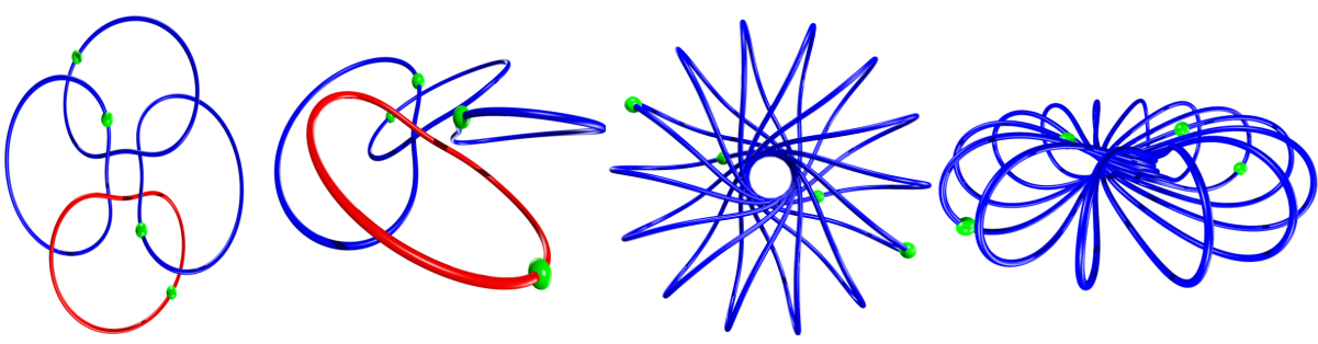
Figure 3: Example result: a choreography in the axial family for the four body problem ($n=4$) with $k=2$ and resonance $p:q=14:9$. The bodies are shown green. The orbit in the rotating frame is illustrated by the left two curves. Far left is top down view of the orbit projected into the $xy$ plane. Second from left is a spatial projection, that is a side view of the torus. The red loop is the segment whose existence is proven by studying the DDE. The remaining three loops are obtained by symmetry. Since the red curve has trivial winding with respect to the $z$-axis, the choreography is a $(14,9)$-torus knot. In particular, since $p,q\neq\pm 1$ the knot is nontrivial in $\mathbb{R}^{3}$. The right two curves are the same orbit transformed back to inertial coordinates so that we see the torus knot choreography. The center right frame is a top down view and the far right is a spatial projection of the choreography.

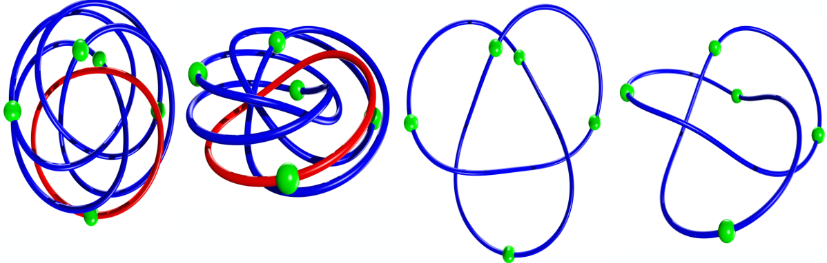
Figure 4: Example result: a choreography in the axial family for the five body problem ($n=5$) with $k=3$ and resonance $p:q=3:1$. Curves from left to right have the same meaning as described in the caption of Figure 3. Due to the nontrivial winding of the red curve around the $z$ axis, the choreography is a (nontrivial) $(3,2)$-torus knot: the trefoil knot mentioned in the introduction. See also Remark 14.

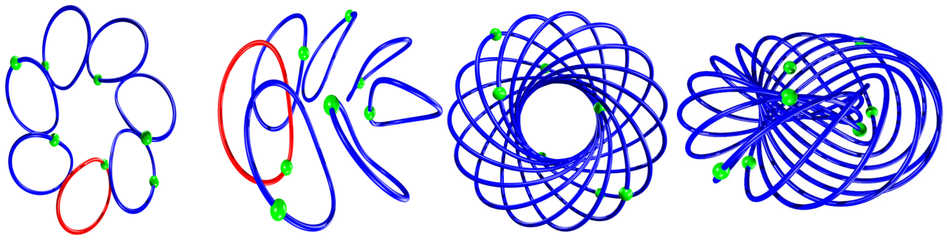
Figure 5: Example result: a choreography in the axial family for the seven body problem ($n=7$) with $k=2$ and resonance $p:q=15:11$. Curves from left to right have the same meaning as described in the caption of Figure 3. Since the red curve has trivial winding with respect to the $z$-axis, the choreography is a $(15,11)$-torus knot. In particular, since $p,q\neq\pm 1$ the knot is nontrivial.

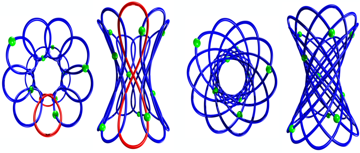
Figure 6: Example result: a choreography along the Lyapunov branch for the nine body problem ($n=9$) with $k=7$ and resonance $p:q=10:13$. Curves from left to right have the same meaning as described in the caption of Figure 3. In this case the solution occurs before the bifurcation to the axial family, hence the orbit shown here is not a torus knot. Rather, the choreography resembles a spatial lissajous figure and illustrates the complexity of the vertical Lyapunov family as the number of bodies increases.

6 Acknowledgments

The authors wish to sincerely thank Sebius Doedel, who provided the numerical data for the $n$-body spatial choreographies computed in [21]. This data is massaged (via Fourier space Newton/continuation schemes we implemented in MatLab) to get appropriate approximate periodic solutions of the DDE, and is the starting point for all the analysis in the present manuscript. This material is based upon work supported by the National Science Foundation under Grant No. 1440140, while R.C. was in residence at the Mathematical Sciences Research Institute in Berkeley, California, during the Fall of 2018. R.C., J.-P.L., and J.D.M.J. were partially supported by a UNAM-PAPIIT project IA102818 and IN101020. C.G.A was partially supported by a UNAM-PAPIIT project IN115019. J.D.M.J was partially supported by NSF grant DMS-1813501. J.-P. L. was partially supported by NSERC.

Appendix

Tables 1, 2, and 3 in this appendix contain numerical data needed in the proofs discussed in the main body of the present work.

$\ell$ $Re((u_{1})_{\ell})$ $Im((u_{1})_{\ell})$ $Re((u_{2})_{\ell})$ $Im((u_{2})_{\ell})$ $Re((u_{3})_{\ell})$ $Im((u_{3})_{\ell})$ $0$ $2.365605595111259$e-01 $0$ $-2.586486484802218$e-11 $0$ $0$ $0$ $1$ $2.730238208518935$e-01 $-8.574371389918268$e-04 $9.594366126621117$e-04 $3.055023346756821$e-01 $3.183998216275582$e-04 $1.013843797046923$e-01 $2$ $2.685276027891537$e-03 $-1.686650070612183$e-05 $-1.686650070615572$e-05 $-2.685276027891251$e-03 $-1.623160460830562$e-04 $-2.584195753881417$e-02 $3$ $-4.758502906990690$e-03 $4.483372035078380$e-05 $-4.483372035075908$e-05 $-4.758502906990715$e-03 $6.528204100190321$e-05 $6.928820000785788$e-03 $4$ $1.883378890295841$e-03 $-2.366033392747678$e-05 $3.143172370973051$e-05 $2.501986861440681$e-03 $-1.766651472817732$e-05 $-1.406266734076041$e-03 $5$ $-5.999006965280112$e-04 $9.420748338183218$e-06 $-1.393289282442757$e-05 $-8.872280378635012$e-04 $6.028392369542407$e-18 $-5.065555035359391$e-18 $6$ $8.811248455572393$e-05 $-1.660505953485738$e-06 $3.309334986825996$e-06 $1.756053477440146$e-04 $2.212344038166846$e-06 $1.173950188081502$e-04 $7$ $8.498774137771074$e-06 $-1.868635687922962$e-07 $-1.868635687932195$e-07 $-8.498774137767349$e-06 $-1.286693928996992$e-06 $-5.852034835941615$e-05 $8$ $-1.218752697705919$e-05 $3.062649564066910$e-07 $-3.062649564072555$e-07 $-1.218752697706007$e-05 $4.623904740337318$e-07 $1.840039558482767$e-05 $9$ $5.555183124075654$e-06 $-1.570568558997190$e-07 $1.997034024758708$e-07 $7.063613764706126$e-06 $-9.561467803603867$e-08 $-3.381941146020149$e-06 $10$ $-1.507114521228540$e-06 $4.734666605843514$e-08 $-7.071044766269389$e-08 $-2.250818294936407$e-06 $3.032901443588402$e-19 $1.295911152109998$e-19 $11$ $2.335200664238406$e-07 $-8.070306668417385$e-09 $1.593213943378485$e-08 $4.610077899825280$e-07 $1.073253754609784$e-08 $3.105536094276917$e-07 $12$ $2.104244568410417$e-08 $-7.933840614338345$e-10 $-7.933840610780110$e-10 $-2.104244568485882$e-08 $-5.811254007216032$e-09 $-1.541283763438269$e-07 $13$ $-3.290905327417571$e-08 $1.344313219810082$e-09 $-1.344313219942516$e-09 $-3.290905327451859$e-08 $1.877957666662263$e-09 $4.597277465765067$e-08 $14$ $1.395325137847766$e-08 $-6.138803968764976$e-10 $7.771252183448973$e-10 $1.766373966056443$e-08 $-3.685236237414536$e-10 $-8.376391836754665$e-09 $15$ $-3.732874395549102$e-09 $1.759771959433038$e-10 $-2.610270876784223$e-10 $-5.536974981491839$e-09 $7.195923927456951$e-20 $7.183652045118199$e-20 $16$ $5.929064335140302$e-10 $-2.981756749601868$e-11 $5.665698400826084$e-11 $1.126593914301232$e-09 $3.809015322039982$e-11 $7.574023856816297$e-10 $17$ $4.804400016695753$e-11 $-2.567445994432811$e-12 $-2.567446178131416$e-12 $-4.804399996475025$e-11 $-1.932234422136176$e-11 $-3.615743781797638$e-10 $18$ $-7.591409192695278$e-11 $4.295939763834585$e-12 $-4.295939829539944$e-12 $-7.591409223386180$e-11 $5.943004126841669$e-12 $1.050195703792485$e-10 $19$ $3.114187654313435$e-11 $-1.860435538023476$e-12 $2.361958845379412$e-12 $3.953689255216923$e-11 $-1.143913421869850$e-12 $-1.914799688503148$e-11 $20$ $-8.409739529661349$e-12 $5.289131681837649$e-13 $-7.792542267774140$e-13 $-1.239017293452956$e-11 $1.543621735017767$e-19 $7.884177072944098$e-21 $21$ $1.333788472823494$e-12 $-8.809217097487679$e-14 $1.640470271719594$e-13 $2.483807275096231$e-12 $1.097557417499826$e-13 $1.661794417444211$e-12 $22$ $1.036015543763710$e-13 $-7.169318194234388$e-15 $-7.169447461203913$e-15 $-1.036016587196382$e-13 $-5.347398762479633$e-14 $-7.727301224303588$e-13 $23$ $-1.573324226886791$e-13 $1.138423940937104$e-14 $-1.138425538834881$e-14 $-1.573324586440305$e-13 $1.631244902296707$e-14 $2.254425161892293$e-13 $24$ $6.514968598200342$e-14 $-4.919794693209673$e-15 $6.284792512394748$e-15 $8.322595890650579$e-14 $-3.120164368146607$e-15 $-4.131838042098719$e-14

Table 1: Fourier coefficients of the trefoil choreography of Theorem 13.

$n=4$, $k=2$ $p:q$ $x_{0}$ $y_{0}$ $z_{0}$ $\dot{x}_{0}$ $\dot{y}_{0}$ $\dot{z}_{0}$ $10:9$ 1.084581210262490 $0.269095117967146$ $-0.400810670225760$ $0.389692393529414$ $-0.222026147390220$ $0.422912633683090$ $6:5$ $1.188423380831879$ $0.396938948763056$ $-0.389381587037265$ $0.556815395497009$ $-0.399232075676175$ $0.462209587632568$ $14:11$ $1.238763513470937$ $0.472974975708732$ $-0.376434682859180$ $0.671427135322320$ $-0.523882170109271$ $0.485529706955392$ $18:13$ $1.282136229445568$ $0.569016024076380$ $-0.350476579202572$ $0.840303451206103$ $-0.707131207512588$ $0.504911385776339$ $10:7$ $1.289649221019265$ $0.602140964327029$ $-0.337606815998459$ $0.906273456937495$ $-0.778064369372037$ $0.505617404253052$ $14:9$ $1.283423571908586$ $0.686295696005838$ $-0.287166965555756$ $1.096549119253133$ $-0.980065341494167$ $0.475381865946370$ $n=5$, $k=3$ $p:q$ $x_{0}$ $y_{0}$ $z_{0}$ $\dot{x}_{0}$ $\dot{y}_{0}$ $\dot{z}_{0}$ $3:1$ $0.781206112370790$ $0.001836389542086$ $0.000409996364153$ $0.005730260732297$ $-2.058041218487896$ $-0.459483910447517$ $n=7$, $k=2$ $p:q$ $x_{0}$ $y_{0}$ $z_{0}$ $\dot{x}_{0}$ $\dot{y}_{0}$ $\dot{z}_{0}$ $15:11$ $0.640762081428200$ $0.304226148803711$ $-0.474444652515547$ $0.561266315985831$ $0.527487897552293$ $-0.391865391782611$ $17:12$ $0.579026084137708$ $0.405193913712767$ $-0.483263936271178$ $0.751751082063471$ $0.635217619217003$ $-0.389409004841267$ $19:13$ $0.542163973849064$ $0.463250571295820$ $-0.484847294002918$ $0.876087261468306$ $0.693625834061019$ $-0.375630471181662$ $23:15$ $0.501902078466474$ $0.521778491863104$ $-0.481735430423762$ $1.042108767392087$ $0.739986909755284$ $-0.348083591542181$ $25:16$ $0.490096168583210$ $0.536730950829510$ $-0.479345448717921$ $1.101770886821142$ $0.747057526841343$ $-0.337802168545392$ $2:1$ $0.388010210558313$ $0.551393376179951$ $-0.422655405682646$ $1.718638435158988$ $0.663687207742979$ $-0.293252731479080$ $n=9$, $k=7$ $p:q$ $x_{0}$ $y_{0}$ $z_{0}$ $\dot{x}_{0}$ $\dot{y}_{0}$ $\dot{z}_{0}$ $10:13$ $0.649289870115096$ $0.307019901740609$ $-0.696068546706640$ $0.621827399858452$ $0.185756061650385$ $-1.139929982269243$ $7:10$ $0.625045716429457$ $0.335012846089124$ $-0.779750789678175$ $0.591061134121929$ $0.198381812020731$ $-1.161246560979217$

Table 2: Initial conditions for the body $u_{n}$ used in the computer-assisted proofs of the torus knot choreographies for different resonances $p:q$ in the $n$-body problem, for $n=4,5,7,9$.

$n=4$, $k=2$ $p:q$ $T$ $m$ $\nu$ $r$ $10:9$ $5.780190889966491$ $30$ $1.1$ $2.5\times 10^{-12}$ $6:5$ $5.352028601820825$ $30$ $1.1$ $1.1\times 10^{-11}$ $14:11$ $5.046198396002492$ $30$ $1.1$ $5.3\times 10^{-11}$ $18:13$ $4.638424788244715$ $50$ $1.1$ $7.1\times 10^{-11}$ $10:7$ $4.495704025529494$ $50$ $1.1$ $1.2\times 10^{-9}$ $14:9$ $4.128707778547495$ $60$ $1.04$ $8.9\times 10^{-8}$ $n=5$, $k=3$ $p:q$ $T$ $m$ $\nu$ $r$ $3:1$ $1.785209272759583$ $25$ $1.03$ $4.7\times 10^{-10}$ $n=7$, $k=2$ $p:q$ $T$ $m$ $\nu$ $r$ $15:11$ $3.035064895370178$ $20$ $1.15$ $4.4\times 10^{-9}$ $17:12$ $2.921452840463272$ $20$ $1.11$ $2.6\times 10^{-8}$ $19:13$ $2.831759112905190$ $40$ $1.07$ $8.7\times 10^{-11}$ $23:15$ $2.699168385210632$ $40$ $1.05$ $7.5\times 10^{-11}$ $25:16$ $2.648783908686700$ $40$ $1.04$ $5.9\times 10^{-11}$ $2:1$ $2.069362428661484$ $50$ $1.04$ $2.8\times 10^{-10}$ $n=9$, $k=7$ $p:q$ $T$ $m$ $\nu$ $r$ $10:13$ $4.479593949184486$ $70$ $1.05$ $4.5\times 10^{-8}$ $7:10$ $4.922630713389546$ $150$ $1.04$ $1.9\times 10^{-9}$

Table 3: Data for the proofs of the torus knot choreographies for different resonances $p:q$ and for $n=4,5,7,9$, in the $n$-body problem.

References

• [1] C Moore. Braids in classical gravity. Physical Review Letters, 70:3675–3679, 1993.
• [2] Alain Chenciner and Richard Montgomery. A remarkable periodic solution of the three-body problem in the case of equal masses. Ann. of Math. (2), 152(3):881–901, 2000.
• [3] Carles Simó. New families of solutions in $N$-body problems. In European Congress of Mathematics, Vol. I (Barcelona, 2000), volume 201 of Progr. Math., pages 101–115. Birkhäuser, Basel, 2001.
• [4] Davide L. Ferrario and Susanna Terracini. On the existence of collisionless equivariant minimizers for the classical $n$-body problem. Invent. Math., 155(2):305–362, 2004.
• [5] V. Barutello and S. Terracini. Action minimizing orbits in the $n$-body problem with simple choreography constraint. Nonlinearity, 17(6):2015–2039, 2004.
• [6] Mitsuru Shibayama. Variational proof of the existence of the super-eight orbit in the four-body problem. Arch. Ration. Mech. Anal., 214(1):77–98, 2014.
• [7] Vivina Barutello, Davide L. Ferrario, and Susanna Terracini. Symmetry groups of the planar three-body problem and action-minimizing trajectories. Arch. Ration. Mech. Anal., 190(2):189–226, 2008.
• [8] Kuo-Chang Chen. Binary decompositions for planar $N$-body problems and symmetric periodic solutions. Arch. Ration. Mech. Anal., 170(3):247–276, 2003.
• [9] Davide L. Ferrario. Symmetry groups and non-planar collisionless action-minimizing solutions of the three-body problem in three-dimensional space. Arch. Ration. Mech. Anal., 179(3):389–412, 2006.
• [10] Davide L. Ferrario and Alessandro Portaluri. On the dihedral $n$-body problem. Nonlinearity, 21(6):1307–1321, 2008.
• [11] Susanna Terracini and Andrea Venturelli. Symmetric trajectories for the $2N$-body problem with equal masses. Arch. Ration. Mech. Anal., 184(3):465–493, 2007.
• [12] Zhiqiang Wang and Shiqing Zhang. New periodic solutions for Newtonian $n$-body problems with dihedral group symmetry and topological constraints. Arch. Ration. Mech. Anal., 219(3):1185–1206, 2016.
• [13] Tomasz Kapela and Carles Simó. Computer assisted proofs for nonsymmetric planar choreographies and for stability of the Eight. Nonlinearity, 20(5):1241–1255, 2007. With multimedia enhancements available from the abstract page in the online journal.
• [14] Tomasz Kapela and Carles Simó. Rigorous KAM results around arbitrary periodic orbits for Hamiltonian systems. Nonlinearity, 30(3):965–986, 2017.
• [15] Tomasz Kapela and Piotr Zgliczyński. The existence of simple choreographies for the $N$-body problem—a computer-assisted proof. Nonlinearity, 16(6):1899–1918, 2003.
• [16] Gianni Arioli, Vivina Barutello, and Susanna Terracini. A new branch of Mountain Pass solutions for the choreographical 3-body problem. Comm. Math. Phys., 268(2):439–463, 2006.
• [17] A. Chenciner and J. Féjoz. Unchained polygons and the $N$-body problem. Regul. Chaotic Dyn., 14(1):64–115, 2009.
• [18] C. García-Azpeitia and J. Ize. Global bifurcation of polygonal relative equilibria for masses, vortices and dNLS oscillators. J. Differential Equations, 251(11):3202–3227, 2011.
• [19] C. García-Azpeitia and J. Ize. Global bifurcation of planar and spatial periodic solutions from the polygonal relative equilibria for the $n$-body problem. J. Differential Equations, 254(5):2033–2075, 2013.
• [20] Jorge Ize and Alfonso Vignoli. Equivariant degree theory, volume 8 of De Gruyter Series in Nonlinear Analysis and Applications. Walter de Gruyter & Co., Berlin, 2003.
• [21] Renato Calleja, Eusebius Doedel, and Carlos García-Azpeitia. Symmetries and choreographies in families that bifurcate from the polygonal relative equilibrium of the $n$-body problem. Celestial Mech. Dynam. Astronom., 130(7):Art. 48, 28, 2018.
• [22] Eusebius Doedel. AUTO: a program for the automatic bifurcation analysis of autonomous systems. Congr. Numer., 30:265–284, 1981.
• [23] Oscar E. Lanford, III. A computer-assisted proof of the Feigenbaum conjectures. Bull. Amer. Math. Soc. (N.S.), 6(3):427–434, 1982.
• [24] Oscar E. Lanford, III. Computer-assisted proofs in analysis. Phys. A, 124(1-3):465–470, 1984. Mathematical physics, VII (Boulder, Colo., 1983).
• [25] Jean-Pierre Eckmann and Peter Wittwer. A complete proof of the Feigenbaum conjectures. J. Statist. Phys., 46(3-4):455–475, 1987.
• [26] J.-P. Eckmann, H. Koch, and P. Wittwer. A computer-assisted proof of universality for area-preserving maps. Mem. Amer. Math. Soc., 47(289):vi+122, 1984.
• [27] Jean-Philippe Lessard. Recent advances about the uniqueness of the slowly oscillating periodic solutions of Wright’s equation. J. Differential Equations, 248(5):992–1016, 2010.
• [28] Gábor Kiss and Jean-Philippe Lessard. Computational fixed-point theory for differential delay equations with multiple time lags. J. Differential Equations, 252(4):3093–3115, 2012.
• [29] Jean-Philippe Lessard. Continuation of solutions and studying delay differential equations via rigorous numerics. In Rigorous numerics in dynamics, volume 74 of Proc. Sympos. Appl. Math., pages 81–122. Amer. Math. Soc., Providence, RI, 2018.
• [30] Roger D. Nussbaum. Periodic solutions of analytic functional differential equations are analytic. Michigan Math. J., 20:249–255, 1973.
• [31] Shane Kepley and J. D. Mireles James. Chaotic motions in the restricted four body problem via Devaney’s saddle-focus homoclinic tangle theorem. J. Differential Equations, 266(4):1709–1755, 2019.
• [32] Jaime Burgos-García, Jean-Philippe Lessard, and J. D. Mireles James. Spatial periodic orbits in the equilateral circular restricted four-body problem: computer-assisted proofs of existence. Celestial Mech. Dynam. Astronom., 131(1):131:2, 2019.
• [33] Jan Bouwe van den Berg, C. M. Groothedde, and Jean-Philippe Lessard. A general method for computer-assisted proofs of periodic solutions in delay differential problems. Submitted, 2020.
• [34] Jean-Philippe Lessard. Computing discrete convolutions with verified accuracy via Banach algebras and the FFT. Appl. Math., 63(3):219–235, 2018.
• [35] Allan Hungria, Jean-Philippe Lessard, and J. D. Mireles James. Rigorous numerics for analytic solutions of differential equations: the radii polynomial approach. Math. Comp., 85(299):1427–1459, 2016.
• [36] Jan Bouwe van den Berg, Jean-Philippe Lessard, and Konstantin Mischaikow. Global smooth solution curves using rigorous branch following. Math. Comp., 79(271):1565–1584, 2010.
• [37] Sarah Day, Jean-Philippe Lessard, and Konstantin Mischaikow. Validated continuation for equilibria of PDEs. SIAM J. Numer. Anal., 45(4):1398–1424 (electronic), 2007.
• [38] Maxime Breden, Jean-Philippe Lessard, and Matthieu Vanicat. Global Bifurcation Diagrams of Steady States of Systems of PDEs via Rigorous Numerics: a 3-Component Reaction-Diffusion System. Acta Appl. Math., 128:113–152, 2013.
• [39] C. Marchal. The family $P_{12}$ of the three-body problem—the simplest family of periodic orbits, with twelve symmetries per period. Celestial Mech. Dynam. Astronom., 78(1-4):279–298 (2001), 2000. New developments in the dynamics of planetary systems (Badhofgastein, 2000).
• [40] Renato Calleja, Eusebius Doedel, Carlos García-Azpeitia, and Carlos L. Pando L. Choreographies in the discrete nonlinear schrödinger equations. The European Physical Journal Special Topics, 227(5-6):615–624, sep 2018.
• [41] Renato C. Calleja, Eusebius J. Doedel, and Carlos García-Azpeitia. Choreographies in the n-vortex problem. Regular and Chaotic Dynamics, 23(5):595–612, sep 2018.
• [42] G. H. Darwin. Periodic Orbits. Acta Math., 21(1):99–242, 1897.
• [43] Forest Ray Moulton. Differential equations. Dover Publications, Inc., New York, N.Y., 1958.
• [44] E. Strömgren. Connaissance actuelle des orbites dans le probleme des trois corps. Bull. Astronom., 9(2):87–130, 1933.
• [45] Victor Szebehely. Theory of Orbits: the restricted problem of three bodies. Academic Press Inc., 1967.
• [46] Gianni Arioli. Branches of periodic orbits for the planar restricted 3-body problem. Discrete Contin. Dyn. Syst., 11(4):745–755, 2004.
• [47] Gianni Arioli. Periodic orbits, symbolic dynamics and topological entropy for the restricted 3-body problem. Comm. Math. Phys., 231(1):1–24, 2002.
• [48] Daniel Wilczak and Piotr Zgliczyński. Heteroclinic connections between periodic orbits in planar restricted circular three body problem. II. Comm. Math. Phys., 259(3):561–576, 2005.
• [49] Daniel Wilczak and Piotr Zgliczynski. Heteroclinic connections between periodic orbits in planar restricted circular three-body problem—a computer assisted proof. Comm. Math. Phys., 234(1):37–75, 2003.
• [50] Maciej J. Capiński and Pablo Roldán. Existence of a center manifold in a practical domain around $L_{1}$ in the restricted three-body problem. SIAM J. Appl. Dyn. Syst., 11(1):285–318, 2012.
• [51] Maciej J. Capiński. Computer assisted existence proofs of Lyapunov orbits at $L_{2}$ and transversal intersections of invariant manifolds in the Jupiter-Sun PCR3BP. SIAM J. Appl. Dyn. Syst., 11(4):1723–1753, 2012.
• [52] Maciej J. Capiński and Piotr Zgliczyński. Beyond the Melnikov method: a computer assisted approach. J. Differential Equations, 262(1):365–417, 2017.
• [53] Maciej J. Capiński and Piotr Zgliczyński. Transition tori in the planar restricted elliptic three-body problem. Nonlinearity, 24(5):1395–1432, 2011.
• [54] Joseph Galante and Vadim Kaloshin. Destruction of invariant curves in the restricted circular planar three-body problem by using comparison of action. Duke Math. J., 159(2):275–327, 2011.
• [55] John C. Urschel and Joseph R. Galante. Instabilities in the Sun-Jupiter-asteroid three body problem. Celestial Mech. Dynam. Astronom., 115(3):233–259, 2013.
• [56] Irmina Walawska and Daniel Wilczak. Validated numerics for period-tupling and touch-and-go bifurcations of symmetric periodic orbits in reversible systems. Commun. Nonlinear Sci. Numer. Simul., 74:30–54, 2019.
• [57] Jonathan Jaquette, Jean-Philippe Lessard, and Konstantin Mischaikow. Stability and uniquness of slowly oscillating periodic solutions to wright’s equation. Journal of Differential Equations, 11:7263–7286, 2017.
• [58] Teruya Minamoto and Mitsuhiro T. Nakao. A numerical verification method for a periodic solution of a delay differential equation. Journal of Computational and Applied Mathematics, 235:870–878, 2010.
• [59] A. Aschwanden, A. Schulze-Halberg, and D. Stoffer. Stable periodic solutions for delay equations with positive feedback—a computer-assisted proof. Discrete Contin. Dyn. Syst., 14(4):721–736, 2006.
• [60] Jonathan Jaquette. A proof of Jones’ conjecture. J. Differential Equations, 266(6):3818–3859, 2019.
• [61] Jan Bouwe van den Berg and Jonathan Jaquette. A proof of Wright’s conjecture. J. Differential Equations, 264(12):7412–7462, 2018.
• [62] Robert Szczelina and Piotr Zgliczyński. Algorithm for Rigorous Integration of Delay Differential Equations and the Computer-Assisted Proof of Periodic Orbits in the Mackey–Glass Equation. Found. Comput. Math., 18(6):1299–1332, 2018.
• [63] Jan Bouwe van den Berg and Jean-Philippe Lessard. Rigorous numerics in dynamics. Notices of the American Mathematical Society, 62(9):1057–1061, 2015.
• [64] J.D. Mireles James and Konstantin Mischaikow. Computational proofs in dynamics. Encyclopedia of Applied Computational Mathematics, 2015.
• [65] Warwick Tucker. Validated numerics. Princeton University Press, Princeton, NJ, 2011. A short introduction to rigorous computations.
• [66] Tomasz Kapela, Marian Mrozek, Daniel Wilczak, and Piotr Zgliczyński. Capd::dynsys: a flexible c++ toolbox for rigorous numerical analysis of dynamical systems. (to appear in Communications in Nonlinear Science and Numerical Simulation), https://arxiv.org/abs/2010.07097, 2020.
• [67] Piotr Zgliczynski. $C^{1}$ Lohner algorithm. Found. Comput. Math., 2(4):429–465, 2002.
• [68] Sarah Day and William D. Kalies. Rigorous computation of the global dynamics of integrodifference equations with smooth nonlinearities. SIAM J. Numer. Anal., 51(6):2957–2983, 2013.
• [69] J.-Ll. Figueras, A. Haro, and A. Luque. Rigorous computer-assisted application of KAM theory: a modern approach. Found. Comput. Math., 17(5):1123–1193, 2017.
• [70] http://cosweb1.fau.edu/~jmirelesjames/torusKnotChoreographies.html. (codes associated with the present work), 2019.
• [71] Jean-Philippe Lessard and J. D. Mireles James. Computer assisted Fourier analysis in sequence spaces of varying regularity. SIAM J. Math. Anal., 49(1):530–561, 2017.
• [72] Ramon E. Moore. Interval analysis. Prentice-Hall Inc., Englewood Cliffs, N.J., 1966.
• [73] S.M. Rump. INTLAB - INTerval LABoratory. In Tibor Csendes, editor, Developments in Reliable Computing, pages 77–104. Kluwer Academic Publishers, Dordrecht, 1999. http://www.ti3.tu-harburg.de/rump/.