Non-Parametric Inference Adaptive to Intrinsic Dimension
Abstract
We consider non-parametric estimation and inference of conditional moment models in high dimensions. We show that even when the dimension of the conditioning variable is larger than the sample size , estimation and inference is feasible as long as the distribution of the conditioning variable has small intrinsic dimension , as measured by locally low doubling measures. Our estimation is based on a sub-sampled ensemble of the -nearest neighbors (-NN) -estimator. We show that if the intrinsic dimension of the covariate distribution is equal to , then the finite sample estimation error of our estimator is of order and our estimate is -asymptotically normal, irrespective of . The sub-sampling size required for achieving these results depends on the unknown intrinsic dimension . We propose an adaptive data-driven approach for choosing this parameter and prove that it achieves the desired rates. We discuss extensions and applications to heterogeneous treatment effect estimation.
1 Introduction
Many non-parametric estimation problems in econometrics and causal inference can be formulated as finding a parameter vector that is a solution to a set of conditional moment equations:
| (1) |
when given i.i.d. samples from the distribution of , where is a known vector valued moment function, is an arbitrary data space, is the feature vector that is included . Examples include non-parametric regression111, where is the dependent variable, and ., quantile regression222 and , for some that denotes the target quantile., heterogeneous treatment effect estimation333, where is a vector of treatments, and ., instrumental variable regression444, where is a treatment, an instrument and ., local maximum likelihood estimation555Where the distribution of admits a known density and . and estimation of structural econometric models (see e.g., Reiss and Wolak (2007) and examples in Chernozhukov et al. (2016, 2018b)). The study of such conditional moment restriction problems has a long history in econometrics (see e.g., Newey (1993); Ai and Chen (2003); Chen and Pouzo (2009); Chernozhukov et al. (2015)). However, the majority of the literature assumes that the conditioning variable is low dimensional, i.e. is a constant as the sample size grows (see e.g., Athey et al. (2019)). High dimensional variants have primarily been analyzed under parametric assumptions on , such as sparse linear forms (see e.g., Chernozhukov et al. (2018a)). There are some papers that address the fully non-parametric setup (see e.g., Lafferty and Wasserman (2008); Dasgupta and Freund (2008); Kpotufe (2011); Biau (2012); Scornet et al. (2015)) but those are focused on the estimation problem, and do not address inference (i.e., constructing asymptotically valid confidence intervals).
The goal of this work is to address estimation and inference in conditional moment models with a high-dimensional conditioning variable. As is obvious without any further structural assumptions on the problem, the exponential in dimension rates of approximately (see e.g., Stone (1982)) cannot be avoided. Thereby estimation is in-feasible even if grows very slowly with . Our work, follows a long line of work in machine learning (Dasgupta and Freund, 2008; Kpotufe, 2011; Kpotufe and Garg, 2013), which is founded on the observation that in many practical applications, even though the variable is high-dimensional (e.g. an image), one typically expects that the coordinates of are highly correlated. The latter intuition is formally captured by assuming that the distribution of has a small doubling measure around the target point .
We refer to the latter notion of dimension, as the intrinsic dimension of the problem. Such a notion has been studied in the statistical machine learning literature, so as to establish fast estimation rates in high-dimensional kernel regression settings (Dasgupta and Freund, 2008; Kpotufe, 2011; Kpotufe and Garg, 2013; Xue and Kpotufe, 2018; Chen and Shah, 2018; Kim et al., 2018; Jiang, 2017). However, these works solely address the problem of estimation and do not characterize the asymptotic distribution of the estimates, so as to enable inference, hypothesis testing and confidence interval construction. Moreover, they only address the regression setting and not the general conditional moment problem and consequently do not extend to quantile regression, instrumental variable regression or treatment effect estimation.
From the econometrics side, pioneering works of Wager and Athey (2018); Athey et al. (2019) address estimation and inference of conditional moment models with all the aforementioned desiderata that are required for the application of such methodologies to social sciences, albeit in the low dimensional regime. In particular, Wager and Athey (2018) consider regression and heterogeneous treatment effect estimation with a scalar and prove -asymptotic normality of a sub-sampled random forest based estimator and Athey et al. (2019) extend it to the general conditional moment settings.
These results have been extended and improved in multiple directions, such as improved estimation rates through local linear smoothing Friedberg et al. (2018), robustness to nuisance parameter estimation error Oprescu et al. (2018) and improved bias analysis via sub-sampled nearest neighbor estimation Fan et al. (2018). However, they all require low dimensional setting and the rate provided by the theoretical analysis is roughly , i.e. to get a confidence interval of length or an estimation error of , one would need to collect samples which is prohibitive in most target applications of machine learning based econometrics.
Hence, there is a strong need to provide theoretical results that justify the success of machine learning estimators for doing inference, via their adaptivity to some low dimensional hidden structure in the data. Our work makes a first step in this direction and provides estimation and asymptotic normality results for the general conditional moment problem, where the rate of estimation and the asymptotic variance depend only on the intrinsic dimension, independent of the explicit dimension of the conditioning variable.
Our analysis proceeds in four parts. First, we extend the results by Wager and Athey (2018); Athey et al. (2019) on the asymptotic normality of sub-sampled kernel estimators to the high-dimensional, low intrinsic dimension regime and to vector valued parameters . Concretely, when given a sample , our estimator is based on the approach proposed in Athey et al. (2019) of solving a locally weighted empirical version of the conditional moment restriction
| (2) |
where captures proximity of to the target point . The approach dates back to early work in statistics on local maximum likelihood estimation (Fan et al., 1998; Newey, 1994; Stone, 1977; Tibshirani and Hastie, 1987). As in Athey et al. (2019), we consider weights that take the form of an average over base weights: , where each is calculated based on a randomly drawn sub-sample of size from the original sample. We will typically refer to the function as the kernel. In Wager and Athey (2018); Athey et al. (2019) is calculated by building a tree on the sub-sample, while in Fan et al. (2018) it is calculated based on the -NN rule on the sub-sample.
Our main results are general estimation rate and asymptotic normality theorems for the estimator (see Theorems 1 and 2), which are stated in terms of two high-level assumptions, specifically an upper bound on the rate at which the kernel “shrinks” and a lower bound on the “incrementality” of the kernel. Notably, the explicit dimension of the conditioning variable does not enter the theorem, so it suffices in what follows to show that and depend only on rather than .
The shrinkage rate is defined as the -distance between the target point and the furthest point on which the kernel places positive weight , when trained on a data set of samples, i.e.,
| (3) |
The shrinkage rate of the kernel controls the bias of the estimate (small implies low bias). The sub-sampling size is a lever to trade off bias and variance; larger achieves smaller bias, since is smaller, but increases the variance, since for any fixed the weights will tend to concentrate on the same data points, rather than averaging over observations. Both estimation and asymptotic normality results require the bias to be controlled through the shrinkage rate.
Incrementality of a kernel describes how much information is revealed about the weight of a sample solely by knowledge of , and is captured by the second moment of the conditional expected weight
| (4) |
The incrementality assumption is used in the asymptotic normality proof to argue that the weights have sufficiently high variance that all data points have some influence on the estimate. From the technical side, we use the Hájek projection to analyze our -statistic estimator. Incrementality ensures that there is sufficiently weak dependence in the weights across a sequence of sub-samples and hence the central limit theorem applies. As discussed, the sub-sampling size can be used to control the variance of the weights, and so incrementality and shrinkage are related. We make this precise, proving that incrementality can be lower bounded as a function of kernel shrinkage, so that having a sufficiently low shrinkage rate enables both estimation and inference. These general results could be of independent interest beyond the scope of this work.
For the second part of our analysis, we specialize to the case where the base kernel is the -NN kernel, for some constant . We prove that both shrinkage and incrementality depend only on the intrinsic dimension , rather than the explicit dimension . In particular, we show that and . These lead to our main theorem that the sub-sampled -NN estimate achieves an estimation rate of order and is also -asymptotically normal.
In the third part, we provide a closed form characterization of the asymptotic variance of the sub-sampled -NN estimate, as a function of the conditional variance of the moments, which is defined as . For example, for the -NN kernel, the asymptotic variance is given by
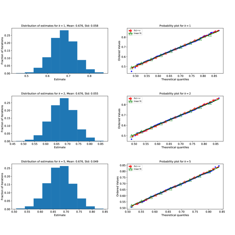
This strengthens prior results of Fan et al. (2018) and Wager and Athey (2018), which only proved the existence of an asymptotic variance without providing an explicit form (and thereby relied on bootstrap approaches for the construction of confidence intervals). Our tight characterization enables an easy construction of plugin normal-based intervals that only require a preliminary estimate of . Our Monte Carlo study shows that such intervals provide very good finite sample coverage in a high dimensional regression setup (see Figure 1)666See Appendix C for detailed explanation of our simulations..
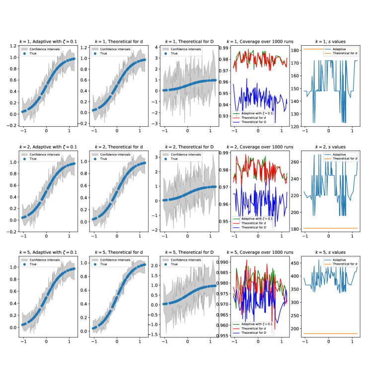
Finally in the last part, we discuss an adaptive data-driven approach for picking the sub-sample size so as to achieve estimation or asymptotic normality with rates that only depend on the unknown intrinsic dimension. This allows us to achieve near-optimal rates while adapting to the unknown intrinsic dimension of data (see Propositions 1 and 2). Figure 2 depicts the performance of our adaptive approach compared to two benchmarks, one constructed based on theory for intrinsic dimension which may be unknown, and the other one constructed naïvely based on the known but sub-optimal extrinsic dimension . As it can be observed from this figure, setting based on intrinsic dimension allows us to build more accurate and smaller confidence intervals, which is crucial for drawing inference in the high-dimensional finite sample regime. Our adaptive approach uses samples to pick very close to the value suggested by our theory and therefore leads to a compelling finite sample coverage777A preliminary implementation of our code is available via http://github.com/khashayarkhv/np_inference_intrinsic..
Our results shed some light on the importance of using adaptive machine learning based estimators, such as nearest neighbor based estimates, when performing estimation and inference in high-dimensional econometric problems. Such estimators address the curse of dimensionality by adapting to a priori unknown latent structure in the data. Moreover, coupled with the powerful sub-sampling based averaging approach, such estimators can maintain their adaptivity, while also satisfying asymptotic normality and thereby enabling asymptotically valid inference; a property that is crucial for embracing such approaches in econometrics and causal inference.
Structure of the paper.
The rest of the paper is organized as follows. In §2, we provide preliminary definitions, in §2.1 and §2.2 we explain our algorithms, in §2.3 we explain doubling dimension (see Appendix B for examples). In §3 we state our assumptions, in §4 we provide general estimation and inference results for kernels that satisfy shrinkage and incrementality conditions, and in §5 we apply such results to the -NN kernel and prove estimation and inference rates for such kernels that only depend on intrinsic dimension. We defer a discussion on the extension to heterogeneous treatment effect estimation and also technical proofs to Appendices.
2 Preliminaries
Suppose we have a data set of observations drawn independently from some distribution over the observation domain . We focus on the case that , where is the vector of covariates and is the outcome. In Appendix D, we briefly discuss how our results can be extended to the setting where nuisance parameters and treatments are included in the model.
Suppose that the covariate space is contained in a ball with unknown diameter . Denote the marginal distribution of by and the empirical distribution of on sample points by . Let be the -ball centered at with radius and denote the standard basis for by .
Let be a score function that maps observation and parameter to a -dimensional score . For and define the expected score as . The goal is to estimate the quantity via local moment condition, i.e.
2.1 Sub-Sampled Kernel Estimation
Base Kernel Learner.
Our learner takes a data set containing observations as input and a realization of internal randomness , and outputs a kernel weighting function . In particular, given any target feature and the set , the weight of each observation in with feature vector is . Define the weighted score on a set with internal randomness as . When it is clear from context we will omit from our notation for succinctness and essentially treat as a random function. For the rest of the paper, we are going to use notations interchangeably.
Averaging over sub-samples of size .
Suppose that we consider random and independent draws from all possible subsets of size and internal randomness variables and look at their average. Index these draws by where contains samples in th draw and is the corresponding draw of internal randomness. We can define the weighted score as
| (5) |
Estimating .
We estimate as a vanishing point of . Letting be this point, then This procedure is explained in Algorithm 1.
2.2 Sub-Sampled -NN Estimation
We specially focus on the case that the weights are distributed across the -NN of . In other words, given a data set , the weights are given according to , where are -NN of in the set . The pseudo-code for this can be found in Algorithm 2.
Complete -statistic.
The expression in Equation (5) is an incomplete -statistic. Complete -statistic is obtained if we allow each subset of size from samples to be included in the model exactly once. In other words, this is achieved if , all subsets are distinct, and we also take expectation over the internal randomness . Denoting this by , we have
| (6) |
Note in the case of -NN estimator we can also represent in terms of order statistics, i.e., is an -statistics (see e.g., Serfling (2009)). By sorting samples in based on their distance with as , we can write where the weights are given by
2.3 Local intrinsic dimension
We are interested in settings that the distribution of has some low dimensional structure on a ball around the target point . The following notions are adapted from Kpotufe (2011), which we present here for completeness.
Definition 1.
The marginal is called doubling measure if there exists a constant such that for any and any we have .
An equivalent definition of this notion is that, the measure is doubling measure if there exist such that for any , and we have .
One example is given by Lebesgue measure on the Euclidean space , where for any we have . Building upon this, let be a subset of -dimensional hyperplane and suppose that for any ball in we have . If is almost uniform, then we also have .
Unfortunately, this global notion of doubling measure is restrictive and most probability measures are globally complex. Rather, once restricted to local neighborhoods, the measure becomes lower dimensional and intrinsically less complex. The following definition captures this intuition better.
Definition 2.
Fix and . The marginal is -homogeneous on if for any we have .
Intuitively, this definition requires the marginal to have a local support that is intrinsically -dimensional. This definition covers low-dimensional manifolds, mixture distributions, -sparse data, and also any combination of these examples. These examples are explained in Appendix B.
3 Assumptions
For non-parametric estimators the bias is connected to the kernel shrinkage, as noted by Athey et al. (2019); Wager and Athey (2018); Oprescu et al. (2018).
Definition 3 (Kernel Shrinkage in Expectation).
The kernel weighting function output by learner when it is given i.i.d. observations drawn from distribution satisfies
Definition 4 (Kernel Shrinkage with High Probability).
The kernel weighting function output by learner when it is given i.i.d. observations drawn from distribution w.p. over the draws of the samples satisfies
As shown in Wager and Athey (2018), for trees that satisfy some regularity condition, for a constant . We are interested in shrinkage rates that scale as , where is the local intrinsic dimension of on . Similar to Oprescu et al. (2018); Athey et al. (2019), we rely on the following assumptions on the moment and score functions.
Assumption 1.
-
1.
The moment corresponds to the gradient w.r.t. of a -strongly convex loss . This also means that the Jacobian has minimum eigenvalue at least .
-
2.
For any fixed parameters , is a -Lipschitz function in for some constant .
-
3.
There exists a bound such that for any observation and any , .
-
4.
The bracketing number of the function class: , satisfies .
Assumption 2.
-
1.
For any coordinate of the moment vector , the Hessian has eigenvalues bounded above by a constant for all .
-
2.
Maximum eigenvalue of is upper bounded by .
-
3.
Second moment of defined as is -Lipschitz in , i.e.,
-
4.
Variogram is Lipschitz: .
The condition on variogram always holds for a that is Lipschitz in . This larger class of functions allows estimation in more general settings such as -quantile regression that involves a which is non-Lipschitz in . Similar to Athey and Imbens (2016); Athey et al. (2019), we require kernel to be honest and symmetric.
Assumption 3.
The kernel , built using samples , is honest if the weight of sample given by is independent of conditional on for any .
Assumption 4.
The kernel , built using samples , is symmetric if for any permutation , the distribution of and are equal. In other words, the kernel weighting distribution remains unchanged under permutations.
For a deterministic kernel , the above condition implies that , for any . In the next section, we provide general estimation and inference results for a general kernel based on the its shrinkage and incrementality rates.
4 Guarantees for sub-sampled kernel estimators
Our first result establishes estimation rates, both in expectation and high probability, for kernels based on their shrinkage rates. The proof of this theorem is deferred to Appendix E.
Theorem 1 (Finite Sample Estimation Rate).
The next result establishes asymptotic normality of sub-sampled kernel estimators. In particular, it provides coordinate-wise asymptotic normality of our estimate around its true underlying value . The proof of this theorem is deferred to Appendix F.
Theorem 2 (Asymptotic Normality).
Let Assumptions 1, 2, 3, and 4 hold. Suppose that Algorithm 1 is executed with and the base kernel satisfies kernel shrinkage, with rate in probability and in expectation. Let be the incrementality of kernel defined in Equation (4) and grow at a rate such that , , and . Consider any fixed coefficient with and define the variance as
Then it holds that . Moreover, suppose that
| (9) |
Then,
Theorems 1 and 2 generalize existing estimation and asymptotic normality results of Athey et al. (2019); Wager and Athey (2018); Fan et al. (2018) to an arbitrary kernel that satisfies appropriate shrinkage and incrementality rates (see Remark 1 in Appendix F). The following lemma relates these two and provides a lower bound on the incrementality in terms of kernel shrinkage. The proof uses the Paley-Zygmund inequality and is left to Appendix G.
Lemma 1.
Corollary 1.
If and satisfies a two-sided version of the doubling measure property on , defined in Definition 2, i.e., for any . Then, .
Even without this extra assumption, we can still characterize the incrementality rate of the -NN estimator, as we observe in the next section.
5 Main theorem: adaptivity of -NN estimator
In this section, we provide estimation guarantees and asymptotic normality of the -NN estimator by using Theorems 1 and 2. We first establish shrinkage and incrementality rates for this kernel.
5.1 Estimation guarantees for the -NN estimator
In this section we provide shrinkage results for the -NN kernel. As observed in Theorem 1, shrinkage rates are sufficient for bounding the estimation error. The shrinkage result that we present in the following would only depend on the local intrinsic dimension of on .
Lemma 2 (High probability shrinkage for the -NN kernel).
Suppose that the measure is -homogeneous on . Then, for any satisfying w.p. at least we have
We can turn this into a shrinkage rate in expectation as follows. In fact, by the very convenient choice of combined with the fact that has diameter , we can establish rate on expected kernel shrinkage. However, a more careful analysis would help us to remove the dependency in the bound and is stated in the following corollary:
Corollary 2 (Expected shrinkage for the -NN kernel).
Suppose that the conditions of Lemma 2 hold. Let be a constant and be the expected shrinkage for the -NN kernel. Then, for any larger than some constant we have .
5.2 Asymptotic normality of the -NN estimator
In this section we prove asymptotic normality of -NN estimator. We start by provide bounds on the incrementality of the -NN kernel.
Lemma 3 (-NN Incrementality).
Let be the -NN kernel and let denote the incrementality rate of this kernel. Then, the following holds:
where sequences and are defined as
We can substitute in Theorem 2 to prove asymptotic normality of the -NN estimator. Before that, we establish the asymptotic variance of this estimator , up to the smaller order terms.
Theorem 4 (Asymptotic Variance of -NN).
Let be one of coordinates. Suppose that is constant while . Then, for the -NN kernel
| (12) |
where and
Theorem 5 (Asymptotic Normality of -NN Estimator).
Plug-in confidence intervals.
Observe that the Theorem 4 implies that if we define as the leading term in the variance, then . Thus, due to Slutsky’s theorem
| (13) |
Hence, we have a closed form solution to the variance in our asymptotic normality theorem. If we have an estimate of the variance of the conditional moment around , then we can build plug-in confidence intervals based on the normal distribution with variance . Note that can be calculated easily for desired values of . For instance, we have and and for the asymptotic variance becomes and respectively.
5.3 Adaptive choice for
According to Theorem 3, picking would trade-off between bias and variance terms. Also, according to Theorem 5, picking with would result in asymptotic normality of the estimator. However, both choices depend on the unknown intrinsic dimension of on the ball . Inspired by Kpotufe (2011), we explain a data-driven way for estimating .
Suppose that is given. Let and pick . For any , let be the -statistic estimator for defined as . Each term in the summation computes the distance of to its -nearest neighbor on and is the average of these numbers over all possible subsets (see Remark 3 in Appendix H regarding to efficient computation of ). Define . Iterate over . Let be the smallest for which we have and let . Note that is decreasing in and is increasing in . Therefore, there exists a unique such that and . We have following results.
Proposition 1 (Adaptive Estimation).
References
- Ai and Chen [2003] Chunrong Ai and Xiaohong Chen. Efficient estimation of models with conditional moment restrictions containing unknown functions. Econometrica, 71(6):1795–1843, 2003.
- Andoni et al. [2017] Alexandr Andoni, Thijs Laarhoven, Ilya Razenshteyn, and Erik Waingarten. Optimal hashing-based time-space trade-offs for approximate near neighbors. In Proceedings of the Twenty-Eighth Annual ACM-SIAM Symposium on Discrete Algorithms, pages 47–66. Society for Industrial and Applied Mathematics, 2017.
- Andoni et al. [2018] Alexandr Andoni, Piotr Indyk, and Ilya Razenshteyn. Approximate nearest neighbor search in high dimensions. arXiv preprint arXiv:1806.09823, 2018.
- Assouad [1983] Patrice Assouad. Plongements lipschitziens dans . Bull. Soc. Math. France, 111:429–448, 1983.
- Athey and Imbens [2016] Susan Athey and Guido Imbens. Recursive partitioning for heterogeneous causal effects. Proceedings of the National Academy of Sciences, 113(27):7353–7360, 2016.
- Athey and Imbens [2017] Susan Athey and Guido W Imbens. The state of applied econometrics: Causality and policy evaluation. Journal of Economic Perspectives, 31(2):3–32, 2017.
- Athey et al. [2018] Susan Athey, Guido W Imbens, and Stefan Wager. Approximate residual balancing: debiased inference of average treatment effects in high dimensions. Journal of the Royal Statistical Society: Series B (Statistical Methodology), 80(4):597–623, 2018.
- Athey et al. [2019] Susan Athey, Julie Tibshirani, and Stefan Wager. Generalized random forests. The Annals of Statistics, 47(2):1148–1178, 2019.
- Belkin and Niyogi [2003] Mikhail Belkin and Partha Niyogi. Laplacian eigenmaps for dimensionality reduction and data representation. Neural computation, 15(6):1373–1396, 2003.
- Bellman [1961] RE Bellman. Adaptive control processes princeton. Press, Princeton, NJ, 1961.
- Belloni et al. [2014a] Alexandre Belloni, Victor Chernozhukov, and Christian Hansen. High-dimensional methods and inference on structural and treatment effects. Journal of Economic Perspectives, 28(2):29–50, 2014a.
- Belloni et al. [2014b] Alexandre Belloni, Victor Chernozhukov, and Christian Hansen. Inference on treatment effects after selection among high-dimensional controls. The Review of Economic Studies, 81(2):608–650, 2014b.
- Belloni et al. [2017] Alexandre Belloni, Victor Chernozhukov, Ivan Fernández-Val, and Christian Hansen. Program evaluation and causal inference with high-dimensional data. Econometrica, 85(1):233–298, 2017.
- Berrett et al. [2019] Thomas B Berrett, Richard J Samworth, Ming Yuan, et al. Efficient multivariate entropy estimation via -nearest neighbour distances. The Annals of Statistics, 47(1):288–318, 2019.
- Biau [2012] Gérard Biau. Analysis of a random forests model. J. Mach. Learn. Res., 13(1):1063–1095, April 2012. ISSN 1532-4435.
- Biau and Devroye [2015] Gérard Biau and Luc Devroye. Lectures on the nearest neighbor method. Springer, 2015.
- Billingsley [2008] Patrick Billingsley. Probability and measure. John Wiley & Sons, 2008.
- Borovkov [2013] A.A. Borovkov. Probability Theory. Springer London, 2013. ISBN 9781447152002.
- Breiman [2001] Leo Breiman. Random forests. Machine learning, 45(1):5–32, 2001.
- Carmo [1992] Manfredo Perdigão do Carmo. Riemannian geometry. Birkhäuser, 1992.
- Chen and Shah [2018] George H. Chen and Devavrat Shah. Explaining the success of nearest neighbor methods in prediction. Foundations and Trends® in Machine Learning, 10(5-6):337–588, 2018. ISSN 1935-8237.
- Chen and Pouzo [2009] Xiaohong Chen and Demian Pouzo. Efficient estimation of semiparametric conditional moment models with possibly nonsmooth residuals. Journal of Econometrics, 152(1):46 – 60, 2009. ISSN 0304-4076. Recent Adavances in Nonparametric and Semiparametric Econometrics: A Volume Honouring Peter M. Robinson.
- Chernozhukov et al. [2015] Victor Chernozhukov, Whitney K. Newey, and Andres Santos. Constrained Conditional Moment Restriction Models. arXiv e-prints, art. arXiv:1509.06311, September 2015.
- Chernozhukov et al. [2016] Victor Chernozhukov, Juan Carlos Escanciano, Hidehiko Ichimura, Whitney K. Newey, and James M. Robins. Locally Robust Semiparametric Estimation. arXiv e-prints, art. arXiv:1608.00033, July 2016.
- Chernozhukov et al. [2018a] Victor Chernozhukov, Denis Chetverikov, Mert Demirer, Esther Duflo, Christian Hansen, Whitney Newey, and James Robins. Double/debiased machine learning for treatment and structural parameters. The Econometrics Journal, 21(1):C1–C68, 2018a.
- Chernozhukov et al. [2018b] Victor Chernozhukov, Denis Nekipelov, Vira Semenova, and Vasilis Syrgkanis. Plug-in regularized estimation of high-dimensional parameters in nonlinear semiparametric models. arXiv preprint arXiv:1806.04823, 2018b.
- Cutler [1993] Colleen D Cutler. A review of the theory and estimation of fractal dimension. In Dimension estimation and models, pages 1–107. World Scientific, 1993.
- Dasgupta and Freund [2008] Sanjoy Dasgupta and Yoav Freund. Random projection trees and low dimensional manifolds. In Proceedings of the fortieth annual ACM symposium on Theory of computing, pages 537–546. ACM, 2008.
- Efron [1982] Bradley Efron. The jackknife, the bootstrap, and other resampling plans, volume 38. Siam, 1982.
- Fan et al. [1998] Jianqing Fan, Mark Farmen, and Irene Gijbels. Local maximum likelihood estimation and inference. Journal of the Royal Statistical Society: Series B (Statistical Methodology), 60(3):591–608, 1998.
- Fan et al. [2018] Yingying Fan, Jinchi Lv, and Jingbo Wang. Dnn: A two-scale distributional tale of heterogeneous treatment effect inference. arXiv preprint arXiv:1808.08469, 2018.
- Friedberg et al. [2018] Rina Friedberg, Julie Tibshirani, Susan Athey, and Stefan Wager. Local linear forests. arXiv preprint arXiv:1807.11408, 2018.
- Friedman et al. [2001] Jerome Friedman, Trevor Hastie, and Robert Tibshirani. The elements of statistical learning, volume 1. Springer series in statistics New York, NY, USA:, 2001.
- Györfi et al. [2006] László Györfi, Michael Kohler, Adam Krzyzak, and Harro Walk. A distribution-free theory of nonparametric regression. Springer Science & Business Media, 2006.
- Hansen [1982] Lars Peter Hansen. Large sample properties of generalized method of moments estimators. Econometrica: Journal of the Econometric Society, pages 1029–1054, 1982.
- Hoeffding [1994] Wassily Hoeffding. Probability inequalities for sums of bounded random variables. In The Collected Works of Wassily Hoeffding, pages 409–426. Springer, 1994.
- Jiang [2017] Heinrich Jiang. Rates of uniform consistency for k-nn regression. arXiv preprint arXiv:1707.06261, 2017.
- Kim et al. [2018] Jisu Kim, Jaehyeok Shin, Alessandro Rinaldo, and Larry Wasserman. Uniform Convergence Rate of the Kernel Density Estimator Adaptive to Intrinsic Dimension. arXiv e-prints, art. arXiv:1810.05935, October 2018.
- Kpotufe [2011] Samory Kpotufe. -nn regression adapts to local intrinsic dimension. In Advances in Neural Information Processing Systems, pages 729–737, 2011.
- Kpotufe and Dasgupta [2012] Samory Kpotufe and Sanjoy Dasgupta. A tree-based regressor that adapts to intrinsic dimension. Journal of Computer and System Sciences, 78(5):1496–1515, 2012.
- Kpotufe and Garg [2013] Samory Kpotufe and Vikas Garg. Adaptivity to local smoothness and dimension in kernel regression. In Advances in neural information processing systems, pages 3075–3083, 2013.
- Lafferty and Wasserman [2008] John Lafferty and Larry Wasserman. Rodeo: Sparse, greedy nonparametric regression. Ann. Statist., 36(1):28–63, 02 2008.
- Lewbel [2007] Arthur Lewbel. A local generalized method of moments estimator. Economics Letters, 94(1):124–128, 2007.
- Mack [1981] Yue-Pok Mack. Local properties of -nn regression estimates. SIAM Journal on Algebraic Discrete Methods, 2(3):311–323, 1981.
- Mackey et al. [2017] Lester Mackey, Vasilis Syrgkanis, and Ilias Zadik. Orthogonal machine learning: Power and limitations. arXiv preprint arXiv:1711.00342, 2017.
- Mullainathan and Spiess [2017] Sendhil Mullainathan and Jann Spiess. Machine learning: an applied econometric approach. Journal of Economic Perspectives, 31(2):87–106, 2017.
- Newey [1993] Whitney K. Newey. 16 efficient estimation of models with conditional moment restrictions. In Econometrics, volume 11 of Handbook of Statistics, pages 419 – 454. Elsevier, 1993.
- Newey [1994] Whitney K Newey. Kernel estimation of partial means and a general variance estimator. Econometric Theory, 10(2):1–21, 1994.
- Oprescu et al. [2018] Miruna Oprescu, Vasilis Syrgkanis, and Zhiwei Steven Wu. Orthogonal random forest for heterogeneous treatment effect estimation. arXiv preprint arXiv:1806.03467, 2018.
- Peel et al. [2010] Thomas Peel, Sandrine Anthoine, and Liva Ralaivola. Empirical bernstein inequalities for u-statistics. In J. D. Lafferty, C. K. I. Williams, J. Shawe-Taylor, R. S. Zemel, and A. Culotta, editors, Advances in Neural Information Processing Systems 23, pages 1903–1911. Curran Associates, Inc., 2010.
- Reiss and Wolak [2007] Peter C Reiss and Frank A Wolak. Structural econometric modeling: Rationales and examples from industrial organization. Handbook of econometrics, 6:4277–4415, 2007.
- Robins and Ritov [1997] James M Robins and Ya’acov Ritov. Toward a curse of dimensionality appropriate (coda) asymptotic theory for semi-parametric models. Statistics in medicine, 16(3):285–319, 1997.
- Roweis and Saul [2000] Sam T Roweis and Lawrence K Saul. Nonlinear dimensionality reduction by locally linear embedding. science, 290(5500):2323–2326, 2000.
- Samworth et al. [2012] Richard J Samworth et al. Optimal weighted nearest neighbour classifiers. The Annals of Statistics, 40(5):2733–2763, 2012.
- Scornet et al. [2015] Erwan Scornet, Gérard Biau, and Jean-Philippe Vert. Consistency of random forests. Ann. Statist., 43(4):1716–1741, 08 2015.
- Serfling [2009] Robert J Serfling. Approximation theorems of mathematical statistics, volume 162. John Wiley & Sons, 2009.
- Staniswalis [1989] Joan G Staniswalis. The kernel estimate of a regression function in likelihood-based models. Journal of the American Statistical Association, 84(405):276–283, 1989.
- Stone [1977] Charles J Stone. Consistent nonparametric regression. The Annals of Statistics, pages 595–620, 1977.
- Stone [1982] Charles J. Stone. Optimal global rates of convergence for nonparametric regression. Ann. Statist., 10(4):1040–1053, 12 1982.
- Tenenbaum et al. [2000] Joshua B Tenenbaum, Vin De Silva, and John C Langford. A global geometric framework for nonlinear dimensionality reduction. Science, 290(5500):2319–2323, 2000.
- Tibshirani and Hastie [1987] Robert Tibshirani and Trevor Hastie. Local likelihood estimation. Journal of the American Statistical Association, 82(398):559–567, 1987.
- Verma et al. [2009] Nakul Verma, Samory Kpotufe, and Sanjoy Dasgupta. Which spatial partition trees are adaptive to intrinsic dimension? In Proceedings of the twenty-fifth conference on uncertainty in artificial intelligence, pages 565–574. AUAI Press, 2009.
- Wager and Athey [2018] Stefan Wager and Susan Athey. Estimation and inference of heterogeneous treatment effects using random forests. Journal of the American Statistical Association, 113(523):1228–1242, 2018.
- Xue and Kpotufe [2018] Lirong Xue and Samory Kpotufe. Achieving the time of -nn, but the accuracy of -nn. In Amos Storkey and Fernando Perez-Cruz, editors, Proceedings of the Twenty-First International Conference on Artificial Intelligence and Statistics, volume 84 of Proceedings of Machine Learning Research, pages 1628–1636, 09–11 Apr 2018.
Appendix A Related work
There exists a vast literature on average treatment effect estimation in high-dimensional settings. The key challenge in such settings is the problem of overfitting which is usually handled by adding regularization terms. However, this leads to a shrinked estimate for the average treatment effect and therefore not desirable. The literature has taken various approaches to solve this issue. For instance, Belloni et al. [2014a, b] used a two-step method for estimating average treatment effect where in the first step feature-selection is accomplished via a lasso and then treatment effect is estimated using selected features. Athey et al. [2018] studied approximate residual balancing where a combination of weight balancing and regression adjustment is used for removing undesired bias and for achieving a double robust estimator. Chernozhukov et al. [2018a, a] considered a more general semi-parametric framework and studied debiased/double machine learning methods via first order Neyman orthogonality condition. Mackey et al. [2017] extended this result to higher order moments. Please refer to Athey and Imbens [2017], Mullainathan and Spiess [2017], Belloni et al. [2017] for a review on this literature.
However, in many applications, researchers are interested in estimating heterogeneous treatment effect on various sub-populations. One effective solution is to use one of the methods described in previous paragraph to estimate problem parameters and then project such estimations onto the sub-population of interest. However, these approaches usually perform poorly when there is a model mis-specification, i.e., when the true underlying model does not belong to the parametric search space. Consequently, researchers have studied non-parametric estimators such as -NN estimators, kernel estimators, and random forests. While these non-parametric estimators are very robust to model mis-specification and work well under mild assumptions on the function of interest, they suffer from the curse of dimensionality (see e.g., Bellman [1961], Robins and Ritov [1997], Friedman et al. [2001]). Therefore, for applying these estimators in high-dimensional settings it is necessary to design and study non-parametric estimators that are able to overcome curse of dimensionality when possible.
The seminal work of Wager and Athey [2018] utilized random forests originally introduced by Breiman [2001] and adapted them nicely for estimating heterogeneous treatment effect. In particular, the authors demonstrated how the recursive partitioning idea, explained in Athey and Imbens [2016] for estimating heterogeneity in causal settings, can be further analyzed to establish asymptotic properties of such estimators. The main premise of random forests is that they are able to adaptively select nearest neighbors and that is very desirable in high-dimensional settings where discarding uninformative features is necessary for combating the curse of dimensionality. In a follow-up work, they extended these results and introduced Generalized Random Forests for more general setting of solving generalized method of moment (GMM) equations Athey et al. [2019]. There has been some interesting developments of such ideas to other settings. Fan et al. [2018] introduced Distributional Nearest Neighbor (DNN) where they used -NN estimators together with sub-sampling and explained that by precisely combining two of these estimators for different sub-sampling sizes, the first order bias term can be efficiently removed. Friedberg et al. [2018] paired this idea with a local linear regression adjustment and introduced Local Linear Forests in order to improve forest estimations for smooth functions. Oprescu et al. [2018] incorporated the double machine learning methods of Chernozhukov et al. [2018a] into GMM framework of Athey et al. [2019] and studied Orthogonal Random Forests in partially linear regression models with high-dimensional controls. Although forest kernels studied in Wager and Athey [2018] and Athey et al. [2019] seem to work well in high-dimensional applications, to the best of our knowledge, there still does not exists a theoretical result supporting it. In fact, all existing theoretical results suffer from the curse of dimensionality as they depend on the dimension of problem .
The literature on machine learning and non-parametric statistics has recently studied how these worst-case performances can be avoided when the intrinsic dimension of problem is smaller than . Please refer to Cutler [1993] for different notions of intrinsic dimension in metric spaces. Dasgupta and Freund [2008] studied random projection trees and showed that the structure of these trees do not depend on the actual dimension , but rather on the intrinsic dimension . They used the notion of Assouad Dimension, introduced by Assouad [1983], and proved that using random directions for splitting, the number of levels required for halving the diameter of a leaf scales as . The follow-up work Verma et al. [2009] generalized these results for some other notions of dimension. Kpotufe and Dasgupta [2012] extended this idea to the regression setting and proved integrated risk bounds for random projection trees that were only dependent on intrinsic dimension. Kpotufe [2011], Kpotufe and Garg [2013] studied this in the context of -NN and kernel estimations and established uniform point-wise risk bounds only depending on the local intrinsic dimension.
Our work is deeply rooted in the literature on intrinsic dimension explained above, literature on -NN estimators (see e.g, Mack [1981], Samworth et al. [2012], Györfi et al. [2006], Biau and Devroye [2015], Berrett et al. [2019], Fan et al. [2018]), and generalized method of moments (see e.g., [Tibshirani and Hastie, 1987, Staniswalis, 1989, Fan et al., 1998, Hansen, 1982, Stone, 1977, Lewbel, 2007, Mackey et al., 2017]). We adapt the framework of Athey et al. [2019] and Oprescu et al. [2018] and solve a generalized moment problem using a DNN estimator, originally introduced and studied by Fan et al. [2018]. We establish consistency and inference properties of this estimator and prove that these properties only depend on the local intrinsic dimension of problem. In particular, we prove that the finite sample estimation error of order together with -asymptotically normality result of DNN estimator for solving the generalized moment problem regardless of how big the actual dimension is.
Our result differs from existing literature on intrinsic dimension (e.g., Kpotufe [2011], Kpotufe and Garg [2013]) since in addition to estimation guarantees for the regression setting, we also allow valid inference in solving conditional moment equations. Our asymptotic normality result is different from existing results for -NN (see e.g., Mack [1981]), generalized method of moments (see e.g., Lewbel [2007]). This paper complements the work of Fan et al. [2018] and extends it to the generalized method of moment setting. Furthermore, we relax the common assumption on the existence of density for covariates and prove that DNN estimators are adaptive to intrinsic dimension.
We also provide the exact expression for the asymptotic variance of DNN estimator built using a -NN kernel, which enables plug-in construction of confidence intervals, rather than the bootstrap method of [Efron, 1982] which was used by [Wager and Athey, 2018, Athey et al., 2019, Fan et al., 2018]. While establishing consistency and asymptotic normality of our estimator, we also provide more general bounds on kernel shrinkage rate and also incrementality which can be useful for establishing asymptotic properties in other applications. One such application is given in high-dimensional settings where the exact nearest neighbor search is computationally expensive and Approximate Nearest Neighbor (ANN) search is often replaced in order to reduce this cost. Our flexible result allows us to use the state-of-the-art ANN algorithms (see e.g., Andoni et al. [2017, 2018]) while maintaining consistency and asymptotic normality.
Appendix B Examples of spaces with small intrinsic dimension
In this section we provide examples of metric spaces that have small local intrinsic dimension. Our first example covers the setting where the distribution of data lies on a low-dimensional manifold (see e.g., Roweis and Saul [2000], Tenenbaum et al. [2000], Belkin and Niyogi [2003]). For instance, this happens for image inputs. Even though images are often high-dimensional (e.g., in the case of by images), all these images belong intrinsically to a -dimensional manifold.
Example 1 (Low dimensional manifold (adapted from Kpotufe [2011])).
Consider a -dimensional submanifold and let have lower and upper bounded density on . The local intrinsic dimension of on is , provided that is chosen small enough and some conditions on curvature hold. In fact, Bishop-Gromov theorem (see e.g., Carmo [1992]) implies that under such conditions, the volume of ball is . This together with the lower and upper bound on the density implies that , i.e. is -homogeneous on for some .
Another example which happens in many applications, is sparse data. For example, in the bag of words representation of text documents, we usually have a vocabulary consisting of words. Although is usually large, each text document contains only a small number of these words. In this application, we expect our data (and measure) to have smaller intrinsic dimension. Before stating this example, let us discuss a more general example about mixture distributions.
Example 2 (Mixture distributions (adapted from Kpotufe [2011])).
Consider any mixture distribution , with each defined on with potentially different supports. Consider a point and note that if , then there exists a ball such that . This is true since the support of any probability measure is always closed, meaning that its complement is an open set. Now suppose that is chosen small enough such that for any satisfying , is -homogeneous on , while for any satisfying we have . Then,
where and and we used the fact that if then . Therefore, is -homogeneous on .
This result applies to the case of -sparse data and is explained in the following example.
Example 3 (-sparse data).
Suppose that is defined as
Let be a probability measure on . In this case, we can write as the union of -dimensonal hyperplanes in . In fact,
Letting be the probability measure restricted to the hyperplane defined by , we can express . Therefore, the result of Example 2 implies that for any , for that is small enough is -homogeneous on .
Our final example is about the product measure. This allows us to prove that any concatenation of spaces with small intrinsic dimension has a small intrinsic dimension as well.
Example 4 (Concatenation under the product measure).
Suppose that is a probability measure on . Define and let be the product measure on , i.e., for that is -measurable, . Suppose that is -homogeneous on and let . Then, is -homogeneous on , where and . To establish this, let and note that for any we have
where we used two simple inequalities that implies and further implies .
Appendix C Simulation Setting
C.1 Single test point
The data for single test point simulation, shown in Figure 1, has been generated as follows. Here , and . All the points are generated using , where and entries of are independently sampled from . Components of each are also generated independently from . We generate a fix test point and keep the matrix throughout all Monte-Carlo iterations fixed. In each Monte-Carlo iteration, we generate training points as mentioned before. The values of are generated according to , where , and with . We are interested in estimate and inference for which is equivalent to solving for with at . We run DNN (Algorithm 2) for and with parameter chosen using Proposition 2 with over Monte-Carlo iterations and report the histogram and quantile-quantile plot of estimates compared to theoretical asymptotic normal distribution of estimates stemming from our characterization. In our simulations, we considered the complete -statistic case, i.e., .
C.2 Multiple test point
The data for the multiple test point simulation, shown in Figure 2, has been generated very similarly to the single test point setting. The only difference is that instead of generating a single test point we generate test points. These test points together with matrix are kept fixed throughout all Monte-Carlo iterations. We compare the performance of DNN (Algorithm 2) with parameter chosen using Proposition 2 with with two benchmarks that set and . This process has been repeated for and and the coverage over a single run for all test points, the empirical coverage over runs, and chosen versus are depicted.
Appendix D Nuisance parameters and heterogeneous treatment effects
Using the techniques of Oprescu et al. [2018], our work also easily extends to the case where the moments depend on, potentially infinite dimensional, nuisance components , that also need to be estimated, i.e.,
| (14) |
If the moment is orthogonal with respect to and assuming that can be estimated on a separate sample with a conditional MSE rate of
| (15) |
then using the techniques of Oprescu et al. [2018], we can argue that both our finite sample estimation rate and our asymptotic normality rate, remain unchanged, as the estimation error only impacts lower order terms. This extension allows us to capture settings like heterogeneous treatment effects, where the treatment model also needs to be estimated when using the orthogonal moment as
| (16) |
where is the outcome of interest, is a treatment, are confounding variables, and . The latter two nuisance functions can be estimated via separate non-parametric regressions. In particular, if we assume that these functions are sparse linear in , i.e.:
| (17) |
Then we can achieve a conditional mean-squared-error rate of the required order by using the kernel lasso estimator of Oprescu et al. [2018], where the kernel is the sub-sampled -NN kernel, assuming the sparsity does not grow fast with .
Appendix E Proof of Theorem 1
Lemma 4.
For any :
| (18) |
Proof.
By strong convexity of the loss and the fact that , we have:
By convexity of the loss we have:
Combining the latter two inequalities we get:
Note that if , then the result is obvious. Otherwise, dividing over by completes the proof of the lemma. ∎
Lemma 5.
Let . Then the estimate satisfies:
| (19) |
Proof.
Observe that , by definition, satisfies . Thus:
∎
Lemma 6.
Suppose that the kernel is built with sub-sampling at rate , in an honest manner (Assumption 3) and with at least sub-samples. If the base kernel satisfies kernel shrinkage in expectation, with rate , then w.p. :
| (20) |
Proof.
Define
where we remind that denotes the complete -statistic:
Here the expectation is taken with respect to the random draws of samples. Then, the following result which is due to Oprescu et al. [2018] holds.
Lemma 7 (Adapted from Oprescu et al. [2018]).
For any and target
In other words, Lemma 7 states that, in the expression for we can simply replace with its expectation which is . We can then express as sum of kernel error, sampling error, and sub-sampling error, by adding and subtracting appropriate terms, as follows:
The parameters should be chosen to trade-off these error terms nicely. We will now bound each of these three terms separately and then combine them to get the final bound.
Bounding the Kernel error.
By Lipschitzness of with respect to and triangle inequality, we have:
where the second to last inequality follows from the fact that .
Bounding the Sampling error.
For bounding the sampling error we rely on Lemma 15 and in particular Corollary 4. Observe that for each , is a complete -statistic for each . Thus the sampling error defines a -process over the class of symmetric functions , with . Observe that since is a convex combination of functions in , the bracketing number of functions in is upper bounded by the bracketing number of , which by our assumption, satisfies . Moreover, by our assumptions on the upper bound of , we have that . Thus all conditions of Corollary 4 are satisfied, with and we get that w.p. :
| (21) |
By a union bound over , we get that w.p. :
| (22) |
Bounding the Sub-sampling error.
Sub-sampling error decays as is increased. Note that for a fixed set of samples , for a set randomly chosen among all subsets of size from the samples, we have:
Therefore, can be thought as the sum of i.i.d. random variables each with expectation equal to , where expectation is taken over draws of sub-samples, each with size . Thus one can invoke standard results on empirical processes for function classes as a function of the bracketing entropy. For simplicity, we can simply invoke Corollary 4 in the appendix for the case of a trivial -process, with and to get that w.p. :
Thus for , the sub-sampling error is of lower order than the sampling error and can be asymptotically ignored. Putting together the upper bounds on sampling, sub-sampling and kernel error finishes the proof of the Lemma. ∎
The probabilistic statement of the proof follows by combining the inequalities in the above three lemmas. The in expectation statement follows by simply integrating the exponential tail bound of the probabilistic statement.
Appendix F Proof of Theorem 2
We will show asymptotic normality of for some arbitrary direction , with . Consider the complete multi-dimensional -statistic:
| (23) |
Let
| (24) |
where (as in the proof of Theorem 1) and
| (25) |
Finally, let
| (26) |
For shorthand notation let , and
be a single dimensional complete -statistic. Thus we can re-write:
We then have the following lemma which its proof is provided in Appendix J:
Lemma 8.
Invoking Lemma 8 and using our assumptions on the kernel, we conclude that:
| (27) |
For some sequence which decays at least as slow as . Hence, since
if we show that , then by Slutsky’s theorem we also have that:
| (28) |
as desired. Thus, it suffices to show that:
| (29) |
Observe that since , we have . Thus it suffices to show that:
Lemma 9.
Under the conditions of Theorem 2, for :
| (30) |
Proof.
Performing a second-order Taylor expansion of around and observing that , we have that for some :
Letting , writing the latter set of equalities for each in matrix form, multiplying both sides by and re-arranging, we get that:
Thus by the definition of we have:
By the bounds on the eigenvalues of and , we have that:
| (31) |
Thus we have:
By our estimation error Theorem 1, we have that the expected value of the second term on the right hand side is of order . Thus by the assumptions of the theorem, both are . Hence, the second term is .
Kernel Error.
Term is a kernel error and hence is upper bounded by in expectation. Since, by assumption is chosen such that , we ge that .
Sub-sampling Error.
Term is a sub-sampling error, which can be made arbitrarily small if the number of drawn sub-samples is large enough and hence . In fact, similar to the part about bounding sub-sampling error in Lemma 6 we have that that:
Therefore, can be thought as the sum of independent random variables each with expectation equal to . Now we can invoke Corollary 4 in the appendix for the trivial U-process, with to get that w.p. :
Hence, for , due to our assumption that we get .
Sampling Error.
Thus it suffices that show that , in order to conclude that . Term can be re-written as:
| (32) |
Observe that each coordinate of , is a stochastic equicontinuity term for -processes over the class of symmetric functions , with . Observe that since is a convex combination of functions in , the bracketing number of functions in is upper bounded by the bracketing number of , which in turn is upper bounded by the bracketing number of the function class , which by our assumption, satisfies . Moreover, under the variogram assumption and the lipschitz moment assumption we have that if , then:
| (Jensen’s inequality) | ||||
| (honesty of kernel) | ||||
Moreover, . Thus we can apply Corollary 4, with and to get that if , then w.p. :
Using a union bound this implies that w.p. we have
By our MSE theorem and also Markov’s inequality, w.p. : , where:
Thus using a union bound w.p. , we have:
To improve readability from here we ignore all the constants in our analysis, while we keep all terms (even or terms) that depend on and . Note that we can even ignore and , because they can go to zero at very slow rate such that terms or even appearing in the analysis grow slower than terms. Now, by the definition of and , as well as invoking the inequality for we have:
| (33) |
Hence, using our Assumption on the rates in the statement of Theorem 2 we get that both of the terms above are . Therefore, . Thus, combining all of the above, we get that:
as desired. ∎
Remark 1.
Our notion of incrementality is slightly different from that of Wager and Athey [2018], as there the incrementality is defined as . However, using the tower law of expectation
For a symmetric kernel the term is equal to and is asymptotically negligible compared to , which usually decays at a slower rate.
Appendix G Lower Bound on Incrementality as Function of Kernel Shrinkage
We give a generic lower bound on the quantity that depends only on the Kernel shrinkage. The bound essentially implies that if we know that the probability that the distribution of ’s assigns to a ball of radius around the target is of order , i.e. we should expect at most a constant number of samples to fall in the kernel shrinkage ball, then the main condition on incrementality of the kernel, required for asymptotic normality, holds. In some sense, this property states that the kernel shrinkage behavior is tight in the following sense. Suppose that the kernel was assigning positive weight to at most a constant number of samples. Then kernel shrinkage property states that with high probability we expect to see at least samples in a ball of radius around . The above assumption says that we should also not expect to see too many samples in that radius, i.e. we should also expect to see at most a constant number of samples in that radius. Typically, the latter should hold, if the characterization of is tight, in the sense that if we expected to see too many samples in the radius, then most probably we could have improved our analysis on Kernel shrinkage and given a better bound that shrinks faster.
G.1 Proof of Lemma 1
By the Paley-Zygmund inequality, for any random variable and for any :
Let . Then, applying the latter to the random variable and observing that by symmetry , yields:
Moreover, observe that by the definition of for some :
This means that at most a mass of the support of in the region can have . Otherwise the overall probability that in the region of would be more than . Thus we have that except for a region of mass , for each in the region : . Combining the above we get:
Thus:
Since was arbitrarily chosen, the latter upper bound holds for any , which yields the result.
G.2 Proof of Corollary 1
Thus applying Lemma 1 with yields:
Observe that:
Hence:
where the last follows by choosing . Combining all the above yields:
Appendix H Proofs of Section 5
H.1 Proof of Lemma 2
For proving this result, we rely on Bernstein’s inequality which is stated below:
Proposition 3 (Bernstein’s Inequality).
Suppose that random variables are i.i.d., belong to and . Let and . Then, for any ,
This also implies that w.p. at least the following holds:
| (34) |
Let be any -measurable set. An immediate application of Bernstein’s inequality to random variables , implies that w.p. over the choice of covariates , we have:
In above, we used the fact that . This result has the following corollary.
Corollary 3.
Define and let be an arbitrary -measurable set. Then, w.p. over the choice of training samples, implies .
Proof.
Define . Then, Bernstein’s inequality in Proposition 3 implies that w.p. we have
Assume that , we want to prove that . Suppose, the contrary, i.e., . Then, by dividing the above equation by we get
Note that since , by letting the above implies that
which as only holds for
This contradicts with , implying the result. ∎
Now we are ready to finish the proof of Lemma 2. First, note that using the definition of -homogeneous measure. Note that for any we have . Replace in above. It implies that for any
| (35) |
Pick according to
Note that for having we need
Therefore, replacing this choice of in Equation (35) implies that . Now we can use the result of Corollary 3 for the choice . It implies that w.p. over the choice of training samples, we have
Note that whenever we have
Therefore, w.p. we have
H.2 Proof of Corollary 2
Lemma 2 shows that for any , such that and , we have that:
Let , which is a constant. Solving for in terms of we get:
for any . Thus, noting that ’s and target both belong to that has diameter , we can upper bound the expected value of as:
Note that for larger than some constant, we have . Thus the first and last terms in the latter summation are of order . We now show that the same holds for the middle term, which would complete the proof. By setting and doing a change of variables in the integral we get:
where is the Gamma function. Since by the properties of the Gamma function , the latter evaluates to: . Since , we have that . Thus the middle term is upper bounded by , which is also of order .
H.3 Proof of Lemma 3
Before proving this lemma we state and prove and auxiliary lemma which comes in handy in our proof.
Lemma 10.
Let denote the mass that the density of the distribution of puts on the ball around with radius , which is a random variable as it depends on . Then, for any the following holds:
Proof.
The proof is an easy consequence of symmetry. Let , then we can write
which simply computes the probability that there are at most other points in the ball with radius . Now, by using the tower law
which holds because of the symmetry. In other words, the probability that sample is among the -NN is equal to . Hence, the conclusion follows. ∎
We can finish the proof of Lemma 3. Define , then we can write
Recall that if denotes the mass that the density of the distribution of puts on the ball around with radius , which is a random variable depending on . Therefore,
Now we can write
Now using Lemma 10 (where is replaced by ) we know that for any value of we have
| (36) |
This implies that for any value of we have . The reason is simple. Note that the above is obvious for using Equation (36). For other values of , we can write Equation (36) for values and . Taking their difference implies the result. Note that this further implies that , as is a constant. Therefore, by plugging this back into the expression of we have
which implies the desired result.
Remark 2.
Note that since we can view as follows: how many different subsets of size can we create from a set of elements if we pick a number and then choose elements from the first half of these elements and elements from the second half. Observe that this process creates all possible sets of size from among the elements, which is equal to .
Furthermore, for and for any , after some little algebra, we have
This implies that the summation appeared in Lemma 11 satisfies
H.4 Proof of Theorem 4
Note that according to Lemma 17, the asymptotic variance , where . Therefore, once we establish an expression for we can finish the proof of this theorem. The following lemma provides such result.
Lemma 11.
Proof.
In this proof for simplicity we let and . Let denote the random variable of the -th closest sample to . For the case of -NN we have that:
Let . Then we have:
Let denote the label of the -th closest point to , excluding sample . Then:
Observe that are all independent of . Hence:
Therefore the variance of is equal to the variance of the first term on the right hand side. Hence:
Where we used the fact that:
| (37) |
Moreover, observe that under the event that , we know that the difference between the closest values and the closest values excluding is equal to the difference between the and . Hence:
where the last equation holds from the fact that for any , conditional on , the random variable is independent of and is equal to in expectation. Under the event , we know that the -th closest point is different from sample . We now argue that up to lower order terms, we can replace with in the last equality:
Observe that:
Moreover, by Jensen’s inequality, Lipschitzness of the first moments and kernel shrinkage:
Hence, for , the latter is . Similarly:
which for is also of order . Combining all the above we thus have:
We now work with the first term on the right hand side. By the tower law of expectations:
By Lipschitzness of the second moments, we know that the second part is upper bounded as:
For it is of . Thus:
Note that Lemma 3 provides an expression for which finishes the proof. ∎
For finishing proof of Theorem 4 we need to prove that is equal to plus lower order terms. This is proved in the following lemma.
Lemma 12.
Suppose that and is fixed. Then
Proof.
Note that for any we have according to Remark 2. For any we have
where we used the fact that and are both bounded above by which is a constant. Hence,
as desired. ∎
H.5 Proof of Theorem 5
The goal is to apply Theorem 2. Note that -NN kernel is both honest and symmetric. According to Lemma 2, we have that for , where and are constants. Corollary 2 also implies that . Furthermore, according to Lemma 3, the incrementality is . Therefore, as goes to we have . Moreover, as , we also get that . We only need to ensure that Equation (9) is satisfied. Note that . Therefore, by dividing terms in Equation (9) it suffices that
Note that due to our Assumption , the last term obviously goes to zero. Also, because of the assumption made in the statement of theorem, the first term also goes to zero. We claim that if the first term goes to zero, the same also holds for the second term. Note that we can write
and since , our claim follows. Therefore, all the conditions of Theorem 2 are satisfied and the result follows.
The second part of result is implied by the first part since if and then .
H.6 Proof of Proposition 1
For proving this lemma, we need two following auxiliary results. Before that we state the Hoeffding’s inequality for -statistics Hoeffding [1994].
Proposition 4.
Suppose that are i.i.d. and is a function that has range . Define . Then, for any
Furthermore, for any , w.p. we have
Lemma 13.
Consider the function defined in Section 5.3 and . Then, w.p. , for all values of we have
Proof.
Note that is the complete -statistic estimator for . For each subset of size from we have
Further, holds for any . Therefore, using Hoeffding’s inequality for -statistics stated in Proposition 4, for any fixed , w.p. we have
Note that for and therefore the above translates to
Taking a union bound over , replacing , and using , implies the result. ∎
Lemma 14.
Consider the selection process mentioned in Section 5.3 and let be the output of this process. Then, w.p. we have
Proof.
Note that using Lemma 13, w.p. , for all values of we have . Now consider three different cases:
-
•
Note that based on the choice of , we have . However, . Hence, which contradicts with the assumption that . Note that this is true since is non-positive for .
-
•
Obviously .
-
•
Note that we have
Hence, . This means that which implies . Therefore, .
This completes the proof. ∎
Now we are ready to finalize the proof of Theorem 1. Note that using the result of Lemma 14, w.p. , we have
This basically means that if , then belongs to . Hence, we have and . Now using Theorem 1, for w.p. we have
Note that . Therefore,
Replacing this in above equation together with a union bound implies that w.p. at least we have
which finishes the first part of the proof. For the second part, note that according to Corollary 2, for the -NN kernel , for a constant . Note that at we have
for a constant . The above implies that
Hence,
Remark 3.
Note that although computation of may look complex as it involves calculation of distance to -nearest neighbor of on all subsets, there is a closed form representation for according to its representation based on -statistic. In fact, by sorting samples based on their distance to , i.e, , we have
Therefore, after sorting training samples, we can compute values of very efficient and fast.
H.7 Proof of Proposition 2
Note that according to Lemma 14, w.p. , the output of process, satisfies
where is the point for which we have . This basically means that . Note that for the -NN kernel we have . As , this also implies that . Also, according to the inequality we have and therefore
and hence . Finally, note that and according to Theorem 2 it suffices that
Note that for any and therefore . For the first term,
Now note that and hence . For the second term, note that again and therefore . Now note that since hence
Finally, for the last term we have and hence
This basically means w.p. , belongs to the interval for which the asymptotic normality result in Theorem 2 holds. As , the conclusion follows.
Appendix I Stochastic Equicontinuity of -statistics via Bracketing
We define here some standard terminology on bracketing numbers in empirical process theory. Consider an arbitrary function space of functions from a data space to , equipped with some norm . A bracket , where consists of all functions , such that . An -bracket is a bracket such that . The bracketing number is the minimum number of -brackets needed to cover . The functions used in the definition of the brackets need not belong to but satisfy the same norm constraints as functions in . Finally, for an arbitrary measure on , let
| (38) |
Lemma 15 (Stochastic Equicontinuity for -statistics via Bracketing).
Consider a function space of symmetric functions from some data space to and consider the -statistic of order , with kernel over samples:
| (39) |
Suppose , and let . Then for , w.p. :
Proof.
Let . Moreover, wlog we will assume that contains the zero function, as we can always augment with the zero function without changing the order of its bracketing number. For , let be a partition of into brackets of diameter at most , with containing a single partition of all the functions. Moreover, we assume that are nested partitions. We can achieve the latter as follows: i) consider a minimal bracketing cover of of diameter , ii) assign each to one of the brackets that it is contained arbitrarily and define the partition of size , by taking to be the functions assigned to bracket , iii) let be the common refinement of all partitions . The latter will have size at most . Moreover, assign a representative function to each partition , with the representative for the single partition at level is the zero function.
Chaining definitions.
Consider the following random variables, where the dependence on the random input is hidden:
for some sequence of numbers , to be chosen later. By noting that and continuously expanding terms by adding and subtracting finer approximations to , we can write the telescoping sum:
For simplicity let , and denote the -process:
| (40) |
Our goal is to bound , with high probability. Observe that since contains only the zero function, then . Moreover, the operator is linear. Thus:
Moreover, by triangle inequality:
We will bound each term in each summand separately.
Edge cases.
The final term we will simply bound it by , since , almost surely. Moreover, the summand in the first term for , we bound as follows. Observe that . But we know that , hence: .
Hence, if we assume that is large enough such that , then the latter term is zero. By the setting of that we will describe at the end, the latter would be satisfied if .
terms.
For the terms in the first summand we have by triangle inequality:
Moreover, observe that:
where we used the fact that the partitions in , have diameter at most , with respect to the norm. Now observe that because the partitions are nested, . Therefore, , almost surely. Moreover, . By Bernstein’s inequality for statistics (see e.g. Peel et al. [2010]) for any fixed , w.p. :
Taking a union bound over the members of the partition, and combining with the bound on , we have w.p. :
| (41) |
terms.
For the terms in the second summand, we have that since the partitions are nested, . Moreover, . Thus, by similar application of Bernstein’s inequality for -statistics, we have for a fixed , w.p. :
As ranges there are at most different functions . Thus taking a union bound, we have that w.p. :
Taking also a union bound over the summands and combining all the above inequalities, we have that w.p. :
Choosing for and , we have for some constant :
Moreover, since , we have:
Combining all the above yields the result. ∎
Corollary 4.
Consider a function space of symmetric functions. Suppose that and . Then for , w.p. :
| (42) |
Proof.
Applying Lemma 15, we get for every , the desired quantity is upper bounded by:
Choosing , yields the desired bound. ∎
Appendix J Proof of Lemma 8
We will argue asymptotic normality of the -statistic defined as:
under the assumption that for any subset of indices of size : and that the kernel satisfies shrinkage in probability with rate such that and . For simplicity of notation we let:
| (43) |
and we then denote:
| (44) |
Observe that we can then re-write our -statistic as:
Moreover, observe that by the definition of , and also
Invoking Lemma 17, it suffices to show that: , where . The following lemma shows that under our conditions on the kernel, the latter property holds.
Lemma 16.
Proof.
Note we can write
Here, is zero mean conditional on and also and are uncorrelated, i.e., . Therefore:
For simplicity of notation let denote the random variable which corresponds to the weight of sample . Note that thanks to the honesty of kernel defined in Assumption 3, is independent of conditional on , for . Hence all the corresponding terms in the summation are zero. Therefore, the expression inside the variance above simplifies to
Moreover, by honesty is independent of conditional on . Thus, the above further simplifies to:
Using , this can be further rewritten as
Note that is uniformly upper bounded by some . Furthermore, by the symmetry of the kernel we have .888Since are all equal to the same value and , we get . Thus the second term in the latter is of order . Hence:
Focusing at the first term and letting , we have:
The goal is to prove that the second term is . For ease of notation let . Then we can bound the second term as:
where we used the fact that , the assumption that is -Lipschitz, the tower rule and the definition of . Furthermore,
which by definition is at most . By putting we obtain
where we invoked our assumption that . Thus we have obtained that:
which is exactly the form of the lower bound claimed in the statement of the lemma. This concludes the proof. ∎
J.1 Hájek Projection Lemma for Infinite Order -statistics
The following is a small adaptation of Theorem 2 of Fan et al. [2018], which we present here for completeness.
Lemma 17 (Fan et al. [2018]).
Consider a -statistic defined via a symmetric kernel :
| (45) |
where are i.i.d. random vectors and can be a function of . Let and . Suppose that is bounded, . Then:
| (46) |
where .
Proof.
The proof follows identical steps as the one in Fan et al. [2018]. We argue about the asymptotic normality of a -statistic:
| (47) |
Consider the following projection functions:
where . Then we define the canonical terms of Hoeffding’s -statistic decomposition as:
Subsequently the kernel of the -statistic can be re-written as a function of the canonical terms:
| (48) |
Moreover, observe that all the canonical terms in the latter expression are un-correlated. Hence, we have:
| (49) |
We can now re-write the statistic also as a function of canonical terms:
Now we define the Hájek projection to be the leading term in the latter decomposition:
| (50) |
The variance of the Hajek projection is:
| (51) |
The Hájek projection is the sum of independent and identically distributed terms and hence by the Lindeberg-Levy Central Limit Theorem (see e.g., Billingsley [2008], Borovkov [2013]):
| (52) |
We now argue that the remainder term: vanishes to zero in probability. The latter then implies that as desired. We will show the sufficient condition of convergence in mean square: . From an inequality due to Wager and Athey [2018]:
Since is bounded by a constant and , by our assumption, we have:
| (53) |
∎