Crystalline symmetry protected helical Majorana modes in the iron pnictides

Abstract

We propose that propagating one-dimensional Majorana fermions will develop in the vortex cores of certain iron-based superconductors, most notably Li(Fe_1-xCo_x)As. A key ingredient of this proposal are the 3D Dirac cones recently observed in ARPES experiments [P. Zhang et al., Nat. Phys. 15, 41 (2019)]. Using an effective Hamiltonian around the $\Gamma-Z$ line we demonstrate the development of gapless one-dimensional helical Majorana modes, protected by $C_{4}$ symmetry. A topological index is derived which links the helical Majorana modes to the presence of monopoles in the Berry curvature of the normal state. We present various experimental consequences of this theory and discuss its possible connections with cosmic strings.

Recent experimental Zhang et al. (2019a, 2018); Wang et al. (2018); Liu et al. (2018); Machida et al. (2018); Kong et al. (2019) and theoretical Wang et al. (2015); Xu et al. (2016); Zhang et al. (2019b) advances suggest that iron-based superconductors (FeSCs) can sustain fractionalized excitations. Building on these ideas, here we propose the emergence of dispersive, helical Majorana states in the flux phase of certain FeSCs.

Twelve years ago, two major discoveries occured in condensed matter physics: the observation of high temperature superconductivity in the iron-pnictides Kamihara et al. (2006); Takahashi et al. (2008) and the discovery of topological insulators (TIs) König et al. (2007). FeSCs have challenged our understanding of strongly correlated electron materials, offering the possibility of practical applications. Topological insulators have transformed our understanding of band physics  Schnyder et al. (2008); Bernevig and Hughes (2013) and have led to the discovery of symmetry protected Weyl and Dirac semimetals Armitage et al. (2018). Remarkably, those materials emulate certain aspects of elementary particle physics in solid state experiments.

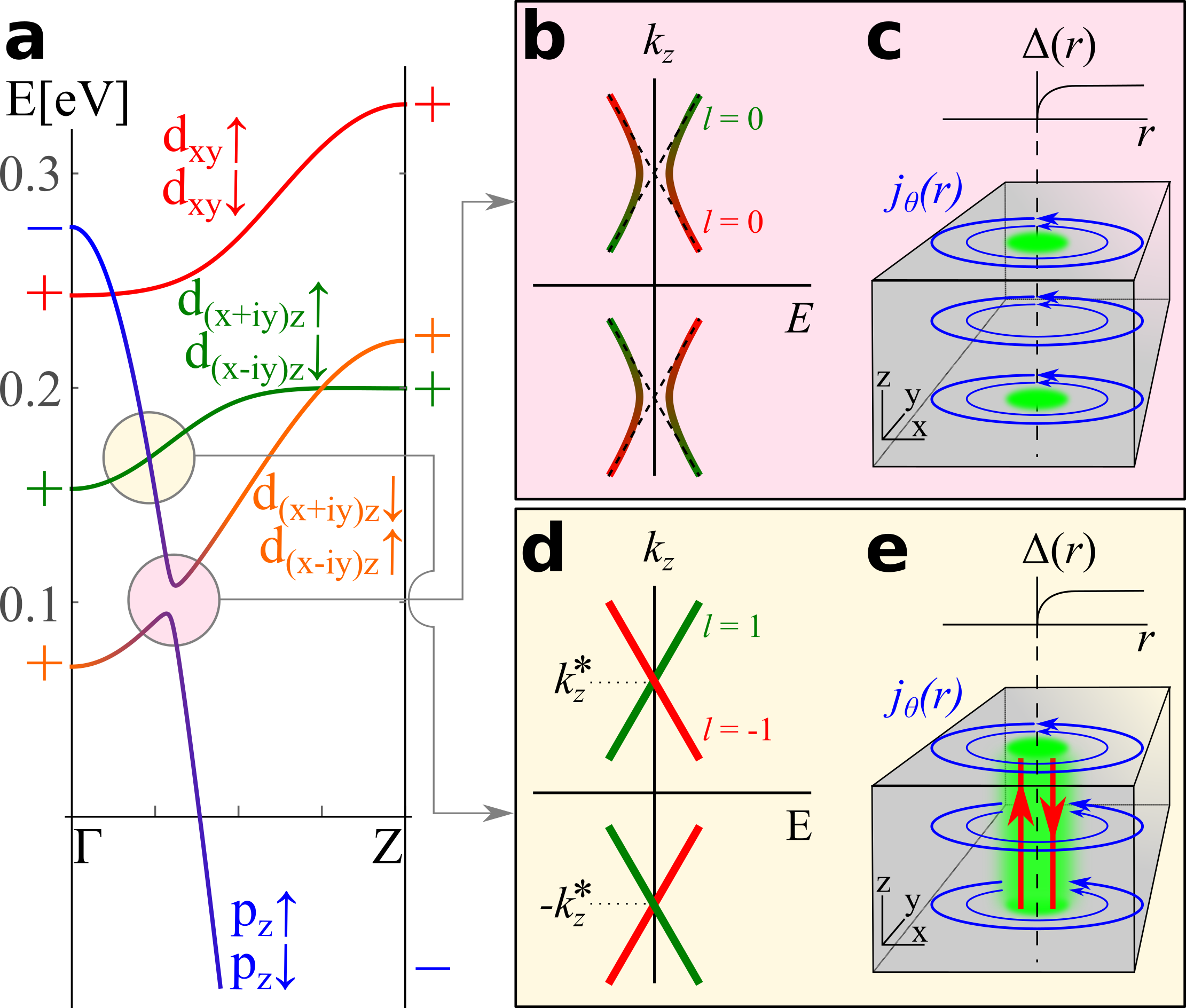
Figure 1: Topology of FeSCs. (a) Band structure in the normal state. For small lattice spacing in c direction, $p_{z}$ orbitals cross the d-states along the $\Gamma$–Z line. When the chemical potential is near the spin-orbit induced gap (marked by a pink disk around 0.1 eV) the ground state is a topological superconductor. (b) In a vortex core, this implies a gapped dispersion of bulk Caroli-Matricon-deGennes states with (c) Majorana zero modes (green pancakes) at the surface termination. At higher doping, when the Fermi energy lies in the vicinity of the Dirac node (marked by a yellow disk around 0.17 eV), (d-e) $C_{4}$ symmetry protects helical Majorana states dispersing along the vortex cores.

Yet despite the excitement in these two new fields, until recently, there has been little overlap between them. Iron based superconductors are layered structures, in which d-orbitals of the iron atoms form quasi-two dimensional bands. The spin-orbit coupling (SOC) in the d-bands was long thought to be too small for topological behavior. However, the recent discovery of marked spin-orbit splitting in photoemission spectra Johnson et al. (2015); Borisenko et al. (2015) has overturned this assumption, with an observation  Wang et al. (2015); Borisenko et al. (2015); Xu et al. (2016); Zhang et al. (2019a) that at small interlayer separations, an enhanced c-axis dispersion drives a topological band inversion between the iron d-bands and ligand $p_{z}$ orbitals. When the chemical potential lies in the hybridization gap between the d and p-bands, the corresponding topological FeSCs sustain Majorana zero modes where-ever magnetic flux lines intersect with the surface, Fig. 1 (c). These excitations have been observed Wang et al. (2018); Liu et al. (2018); Machida et al. (2018); Kong et al. (2019). Here we demonstrate that on additional doping, topological behavior is expected to give rise to dispersive, helical Majorana fermions, Fig. 1 (e) along the cores of superconducting vortices. Observation of these excitations would provide an important confirmation of the topological character of iron based superconductors, yielding a new setting for the realization of Majorana fermions.

Helical Majorana fermions in one dimension correspond to a pair of gapless counter-propagating fermionic excitations, first proposed as excitations within the “$o-$” vortices of superfluid ³He-B  Misirpashaev and Volovik (1995). Whilst these excitations have not been observed, possibly because the energetics of ³He-B favors less symmetric $v-$vortices Vollhardt and Wölfle (2013); Volovik (2003), which do not support helical Majorana modes, we here propose an alternative realization in FeSCs. Recent experimental advances (Table  1) provide evidence for chiral (i.e. unidirectional) Majorana modes at the boundaries of various two dimensional systems, including superconducting-quantum anomalous Hall heterostructures He et al. (2017), 5/2 fractional quantum Hall statesBanerjee et al. (2018) and the layered Kitaev material $\alpha$-RuCl₃ Kasahara et al. (2018).

		boundary of 2D systems		vortex in 3D system
chiral	Exp. Th.	QAH-SC He et al. (2017), $\alpha$-RuCl3 Kasahara et al. (2018), $\nu=5/2$ QH Banerjee et al. (2018) $p+ip$ SC Volovik (1988) (Sr2RuO4 Rice and Sigrist (1995)?) [AZ cl. D Schnyder et al. (2008)]	Exp. Th.	N/A TI-SC heterostructure Meng and Balents (2012)[Weyl SSM]
helical	Exp. Th.	N/A NCS Tanaka et al. (2009); Sato and Fujimoto (2009); Roy (2008); Qi et al. (2009), $s_{\pm}$ SC+SOC Zhang et al. (2013) [AZ cl. DIII Schnyder et al. (2008)]	Exp. Th.	N/A 3He-B Misirpashaev and Volovik (1995), LiFe1-xCoxAs (this work) [Dirac SSM]

Table 1: Phases of matter which sustain 1+1D helical or chiral Majorana fermions. We present all experimental evidence, the first material specific theoretical proposal and generic classes of systems (in square brackets). We omitted Majorana modes which occur at fine-tuned critical points, e.g. at topological phase transitions Hosur et al. (2011); Xu et al. (2016) or at S-TI-S junctions with flux $\pi$  Fu and Kane (2008). Abbreviations: “AZ cl.” = “Altland-Zirnbauer class”, “Exp.” = “Experiment”, “NCS” = “non-centrosymmetric superconductor”, “QAH” = “Quantum anomalous Hall”, “QH” = “Quantum Hall”, “SC”=“superconductor”, “SSM” = “superconducting semimetal”, “Th.” = “Theory”.

Majorana modes in FeSC. Here we summarize the main physics leading to the appearance of helical Majorana subgap states in the flux phase of FeSC, when the magnetic field is aligned in c direction. We shall concentrate on a case where the vortex core size, (determined by the coherence length), is much larger than the lattice spacing, so that vortex-induced interpocket scattering can be neglected. This permits us to concentrate on the region of the Brillouin zone (BZ) which harbors the topological physics, in this case the $\Gamma-Z$ line.

Along this line, the relevant electronic states are classified by the $z-$component of their total angular momentum $J_{z}=L_{z}+S_{z}$. We may exploit the fact that the low energy Hamiltonian close to the $\Gamma-Z$ line Xu et al. (2016); Zhang et al. (2019a); Sup features an emergent continuous rotation symmetry. Three pairs of states are important, $\ket{d_{(x+iy)z}\downarrow},\ket{d_{(x-iy)z}\uparrow}$ (with $j_{z}=\pm 1/2$), $\ket{p_{z},\uparrow},\ket{p_{z},\downarrow}$ (also $j_{z}=\pm 1/2$) and $\ket{d_{(x+iy)z}\uparrow},\ket{d_{(x-iy)z}\downarrow}$ ($j_{z}=\pm 3/2$). Their dispersion is shown in Fig. 1 along with the $d_{xy}$ bands, we used the low energy model of Ref. Xu et al. (2016).

We briefly recapitulate the appearance of localized Majorana zero modes. The $j_{z}=\pm 1/2$ $p_{z}$ states can hybridize with the corresponding $\ket{d_{(x+iy)z}\downarrow},\ket{d_{(x-iy)z}\uparrow}$ states at intermediate $k_{z}$, leading to an avoided crossing of the bands [pink circle at 0.1 eV in Fig. 1 a)]. Since the $p$ and $d$ orbitals carry opposite parity, the band-crossing leads to a parity inversion at the the Z-point. The system is therefore topological Fu and Kane (2007). In the superconducting state, this system is then expected Fu and Kane (2008) to host topological surface superconductivity, developing localized Majorana zero modes at the surface termination of a vortex, Fig. 1 c). These Majorana zero modes can be alternatively interpreted as the topological end states of a fully gapped, 1D superconductor inside the vortex core Xu et al. (2016). In the bulk, where $k_{z}$ is a good quantum number the vortex hosts fermionic subgap states for each $k_{z}$ near the normal state Fermi surface, Fig. 1 b). In particular, the lowest lying states carry angular momentum $l=0$ and develop a topological hybridization gap upon inclusion of SOC.

However, bulk FeSCs can also support dispersive helical Majorana modes in their vortex cores. To see this, we now turn to the situation where the chemical potential lies near the Dirac cone, highlighted by a yellow circle at about 0.17 eV in Fig. 1 a). At this energy, semimetallic Dirac states are observed in ARPES Zhang et al. (2019a): these occur because the different $j_{z}$ quantum numbers of $\ket{p_{z},\uparrow},\ket{p_{z},\downarrow}$ and $\ket{d_{(x+iy)z}\uparrow},\ket{d_{(x-iy)z}\downarrow}$ prevent a hybridization on the high symmetry line leading to a Hamiltonian of the (tilted) Dirac form $H(\textbf{{k}})=H_{+}(\textbf{{k}})\oplus H_{-}(\textbf{{k}})$ Zhang et al. (2019a); Sup ,

$$H_{\pm}(\textbf{{k}})=\left(\begin{array}[]{cc}M_{p}(k_{z})&\pm vk_{x}+ivk_{y}\\ \pm vk_{x}-ivk_{y}&M_{d}(k_{z})\end{array}\right),$$ (1)

where $H_{+}(\textbf{{k}})$ ($H_{-}(\textbf{{k}})$) acts in the subspace of positive (negative) helicity spanned by $\ket{p_{z},\uparrow},\ket{d_{(x+iy)z}\uparrow}$ $(\ket{p_{z},\downarrow},\ket{d_{(x-iy)z}\downarrow})$. The dispersion $M_{p}(k_{z}),M_{d}(k_{z})$ of the relevant $p$ and $d$ orbitals is plotted in Fig. 1 a) and $v$ is the transverse velocity.

We now assume that below $T_{c}$, a spin-singlet, s-wave superconducting phase develops. In an Abrikosov lattice of vortex lines, translational symmetry allows to solve the problem at each $k_{z}$ separately. At the particular values of $k_{z}=\pm k_{z}^{*}$, where $M_{p}(\pm k_{z}^{*})=M_{d}(\pm k_{z}^{*})$, $H_{+}$ and $H_{-}$ separately take the form of a TI surface state. Consequently Fu and Kane (2008), for each helicity a non-degenerate Majorana zero mode appears in each vortex. Now in contrast to the case of Fig. 1 b), these two modes carry different angular momenta $l=\pm 1$ so that they can not be mixed by any perturbation which respects the $C_{4}$ symmetry. This leads to the gapless linear helical dispersion near $\pm k_{z}^{*}$.

Topological origin of helical Majorana modes. The crystalline topological protection of the helical Majorana modes in the flux phase of FeSC can be understood as follows. First, we note that in the normal state, crystalline symmetries, in particular $C_{4}$, impose the decoupling of Hamiltonian (1) into the direct sum of two decoupled helical sectors. Within $H_{+}$ ($H_{-}$), two Weyl points of opposite topological charge $\pm 1$ ($\mp 1$) appear at $(0,0,\pm k_{z}^{*})$, Fig. 2 a). Since crystalline symmetry ensures perfect decoupling, it is favorable to concentrate on a given sector in these explanations and superimpose both sectors in the end. The Berry flux connecting the two Weyl points implies a quantum anomalous Hall state for $k_{z}\in(-k_{z}^{*},k_{z}^{*})$ Foo . The resulting family of chiral edge states forms a Fermi arc in the surface BZ, Fig. 2 b,c). In view of their chiral nature, Fermi arc states can only terminate at a $k_{z}$ which sustains critical bulk states - i.e. at the projection of the Weyl points. From the boundary perspective, their presence is ensured by the topological phase transition at $\pm k_{z}^{*}$.

We now turn to the superconducting case in the flux phase, for which a vortex core represents a normal state cylinder inside of a fully gapped superconducting background. At each $k_{z}\in(-k_{z}^{*},k_{z}^{*})$ the boundary of the vortex core resembles an interface between quantum anomalous Hall state and topological superconductor. This leads to a chiral Majorana encircling the cylinder - i.e. the Majorana analog Zhang et al. (2019a); Yang et al. (2014) of Fermi arc states (purple circles, Fig. 2, d). As explained above, edge states may only disappear as a function of $k_{z}$ when the bulk is critical, therefore it follows that topologically protected vortex core subgap states must cross the Fermi energy at $\pm k_{z}^{*}$.

We conclude this discussion with three remarks. (1) For typical vortex core diameters $\xi$ the chiral Majorana edge states are gapped by finite size effects, yet the above topological argument is still valid, Fig. 2 e). In particular, as in the case of a 3D TI surface, the magnetic flux prevents the critical bulk (= vortex core) states at $\pm k_{z}^{*}$ from gapping. A different situation occurs in ³He-A, where the conservation of the spin projection protects the non-dispersive Fermi arc states for all $k_{z}$ between the projection of Weyl points Volovik (2003); Volovik2011 ; Sup . (2) Taking into account that $H_{+}$ and $H_{-}$ sectors have opposite helicity, the actual state for $k_{z}\in(-k_{z}^{*},k_{z}^{*})$ is a quantum spin Hall insulator, and Fermi arc states are helical rather than chiral. (3) For weak misalignment of the flux line and the c-axis, mixing between decoupled helical sectors $H_{\pm}$ is negligible. Under this assumption, the topological protection of helical modes persists.

Bogoliubov-deGennes (BdG) Hamiltonian. To confirm these heuristic arguments, we have perturbatively diagonalized Sup the BdG Hamiltonian of a topological FeSC with a single vortex. Here, we concentrate on states near $k_{z}^{*}$ and employ a simplified Hamiltonian $\mathcal{H}=\mathcal{H}_{+}\oplus\mathcal{H}_{-}$, where

$$\mathcal{H}_{\pm}=(H_{\pm}-\mu)\tau_{z}+\Delta(\textbf{{r}})\tau_{+}+\Delta^{*}(\textbf{{r}})\tau_{-}.$$ (2)

The Fermi energy $\mu$ is measured from the Dirac point, $\Delta(\textbf{{r}})=|\Delta(r)|e^{i\theta}$ is the superconducting gap ($|\Delta(\infty)|\equiv\Delta$) and $\tau_{x,y,z}$ are Pauli matrices in Nambu space and $\tau_{\pm}=(\tau_{x}\pm i\tau_{y})/2$. Assuming circularly symmetric vortices, we expand the wave function in angular momenta, seeking solutions of the form $\Psi_{\pm}=\sum_{l}e^{ik_{z}z+il\theta}U_{\pm}(\theta)\Psi_{\pm}^{(l)}(r,k_{z})$, where the precise form of the diagonal matrices $U_{\pm}(\theta)$ is given in the supplement. At $l=\pm 1$ a chiral symmetry in the $l$-th sector $\mathcal{H}_{\pm}^{(l)}$ allows us to explicitly construct an unpaired zero energy solution $\Psi_{\pm}^{(\pm 1)}(r,k_{z}^{*})$ in each helical sector. We use these solutions to perturbatively include momenta $k_{z}-k_{z}^{*}$, a Zeeman field $g\mu_{B}B/2$ and orbital dependent gaps $\Delta_{p}-\Delta_{d}=\delta\Delta\neq 0$. By projecting onto the low-energy space we obtain the effective dispersions

$$E_{\pm}(k_{z})=\pm[v_{M}(k_{z}-k_{z}^{*})-w_{M}\delta\Delta+g\mu_{B}B/2].$$ (3)

This confirms the heuristic argument for the appearance of helical Majorana modes and demonstrates that perturbations merely shift $k_{z}^{*}$. A similar result holds near $-k_{z}^{*}$, so that in total two pairs of helical Majorana modes occur, Fig. 1 d). In the limit $\mu\gg\Delta$ we obtain $v_{M}\sim\Delta^{2}\partial_{k_{z}^{*}}[M_{d}(k_{z}^{*})-M_{p}(k_{z}^{*})]/\mu^{2}$ and $w_{M}\sim\Delta/\mu$. The velocity of helical Majorana modes in vortices of ³He - B has an analogous parametrical dependence Misirpashaev and Volovik (1995).

Index theorem. We now demonstrate the link between the helical Majorana modes and the Berry flux between the two pairs of Weyl points, Fig. 2. While several topological invariants were proposed Weinberg (1981); Teo and Kane (2010); Qi et al. (2013); Roy and Goswami (2014) to describe dispersive Majorana modes, we here employ a generalization of an index introduced by Volovik Volovik (1989) for vortices in ³He. Our index measures the imbalance between the number of states of opposite helicity at a given momentum $k_{z}$, $N(k_{z})=[N_{-}(k_{z})-N_{+}(k_{z})]/2$, where

$$N_{\pm}(k_{z})=\sum_{n}\theta[-E_{n}^{\pm}(k_{z})]=\text{Im}\int_{-\infty}^{0}\frac{d\omega}{\pi}\text{Tr}[\mathcal{G}_{\pm}(\omega-i0)]e^{\omega 0^{+}}$$ (4)

counts the number of states with given helicity in the Fermi sea ($\mathcal{G}_{\pm}(z)=[z-\mathcal{H}_{\pm}(k_{z})]^{-1}$ and $n$ labels quantum numbers). In a fully gapped system $N(k_{z})$ is constant as a function of $k_{z}$. In contrast, the presence of helical Majorana modes, Fig. 1 d), implies a jump $N(k_{z}^{*}+0^{+})-N(k_{z}^{*}-0^{-})=1$.

We now relate $N(k_{z})$ to the quantized spin Hall conductivity at a given $k_{z}$ using a semiclassical expansion, which is valid for smoothly varying $\Delta(\textbf{{r}})$. In the eigenbasis of the normal state Hamiltonian $H_{\pm}({\textbf{{p}}})\ket{u_{\textbf{{p}},\xi,\pm}}=\epsilon_{\xi,\pm}(\textbf{{p}})\ket{u_{\textbf{{p}},\xi,\pm}}$ the BdG Hamiltonian in each band takes the form $\mathcal{H}_{\xi,\pm}=\textbf{{d}}_{\xi,\pm}\cdot\bm{\tau}$ (where the transverse components of d describe intraorbital pairing). In the following argument, we drop the band and helicity indices $\xi$ and $\pm$ and employ a Wigner transform Sup ; König and Levchenko so that $\textbf{{d}}(\textbf{{R}},\textbf{{P}})=(\text{Re}\Delta(\textbf{{R}}),-\text{Im}\Delta(\textbf{{R}}),\epsilon(\textbf{{P}})-\mu)$. Due to the algebra of Pauli matrices, the Green’s function $\mathcal{G}(\omega;\textbf{{R}},\textbf{{P}})=[\omega-\textbf{{d}}\cdot\bm{\tau}]^{-1}$ contains a commutator of operator convolutions (denoted by $\circ$)

$$\mathcal{G}(\omega;\textbf{{R}},\textbf{{P}})=(\omega+\textbf{{d}}\cdot\tau)\circ[\omega^{2}-\textbf{{d}}^{2}-\frac{i}{2}\epsilon_{abc}[d_{a}\overset{\circ}{,}d_{b}]\tau_{c}]^{-1}.$$ (5)

The gradient expansion of the convolution is

$$[d_{a}\overset{\circ}{,}d_{b}](\textbf{{R}},\textbf{{P}}) \simeq i\left(\vec{\nabla}_{X}d_{a}\cdot\vec{\nabla}_{P}d_{b}-\vec{\nabla}_{P}d_{a}\cdot\vec{\nabla}_{X}d_{b}\right)$$

$$+i\Omega_{z}\hat{e}_{z}\cdot\left(\vec{\nabla}_{X}d_{a}\times\vec{\nabla}_{X}d_{b}\right).$$ (6)

Here, $\Omega_{z}=i\braket{\partial_{p_{x}}u_{\textbf{{p}}}}{\partial_{p_{y}}u_{\textbf{{p}}}}-i\braket{\partial_{p_{y}}u_{\textbf{{p}}}}{\partial_{p_{x}}u_{\textbf{{p}}}}$ is the Berry curvature. Note that within our gauge invariant formalism, the semiclassical coordinates $\textbf{{R}},\textbf{{P}}$ are kinematic – this leads to the appearance of $\Omega_{z}$ in addition to the Poisson bracket Al’tshuler (1978).

We evaluate $N(k_{z})$ for an isotropic vortex of winding $\nu_{v}$ to leading order in gradients. The vortex enters Eq. (6) as $\vec{\nabla}_{X}d_{y}\times\vec{\nabla}_{X}d_{x}=\nu_{v}\hat{e}_{z}[\partial_{R}|\Delta(R)|^{2}]/2R$. Performing the radial integration and restoring the band and helicity indices, leads to the result $N_{\pm}(k_{z})=-\nu_{v}\sigma_{xy,\pm}(k_{z})$, where

$$\sigma_{xy}^{\pm}(k_{z})=\sum_{\xi}\int\frac{dk_{x}dk_{y}}{2\pi}\Omega^{\xi,\pm}_{z}(\textbf{{k}})\theta(-\epsilon_{\xi,\pm}(\textbf{{k}})).$$ (7)

In this expression, $\Omega^{\xi,\pm}_{z}(\textbf{{k}})$ and $\epsilon_{\xi,\pm}$ are evaluated in the plane at constant $k_{z}$. It follows that $N(k_{z})=\nu_{v}[\sigma^{+}_{xy}(k_{z})-\sigma^{-}_{xy}(k_{z})]/2$ is given by the normal state spin Hall conductivity which establishes the topological origin of the jump in the Fermi surface volume, Fig. 2 f).

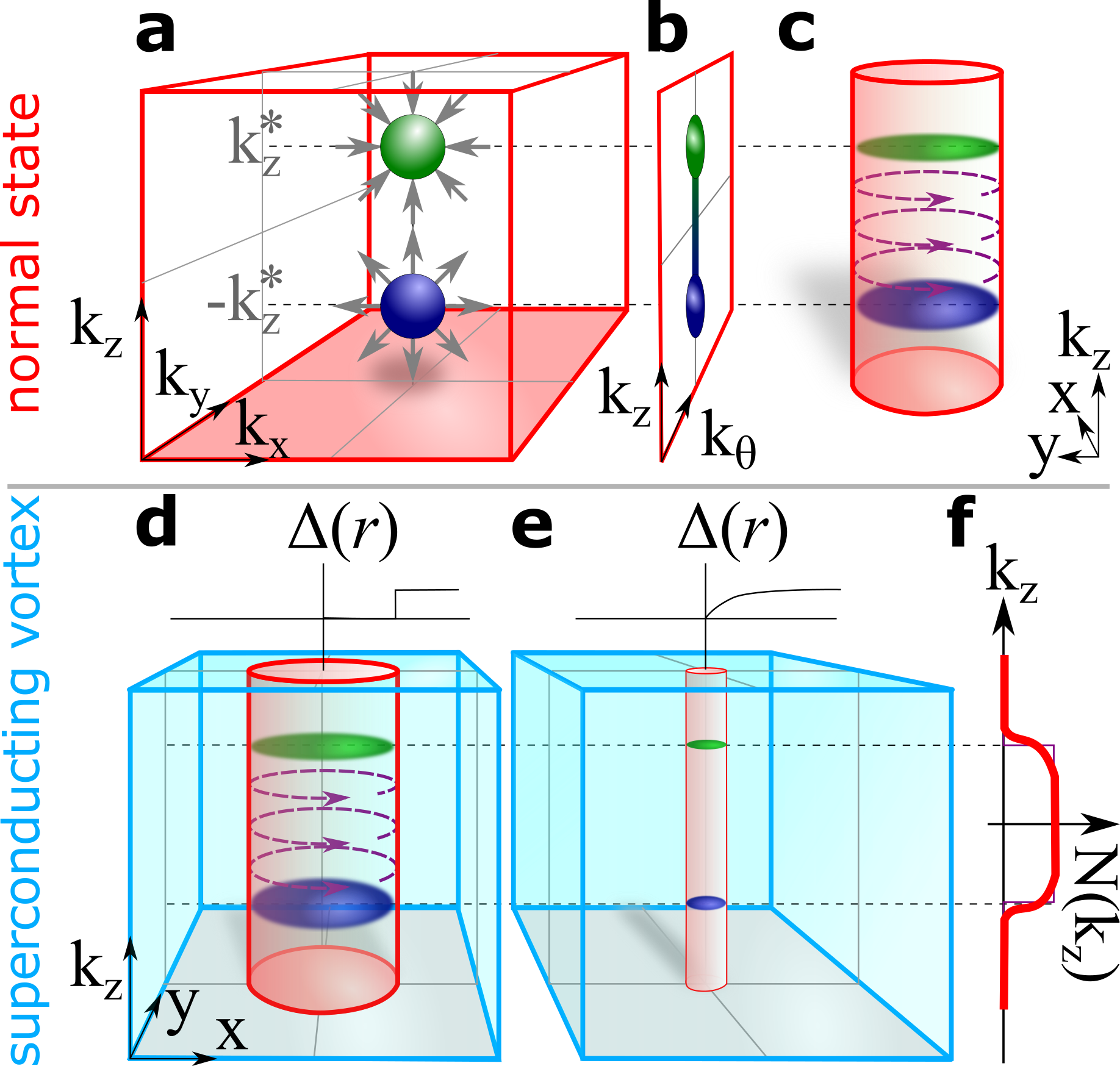
Figure 2: Topological origin of helical Majorana modes. (a) Normal state BZ with helicity resolved Weyl nodes. (b) Surface BZ and Fermi arc. (c) Partial real space representation of a cylindrical Weyl semimetal. Fermi arc states (purple circles) terminate at topological transitions at $\pm k_{z}^{*}$ with delocalized, critical bulk states (green and blue pancakes). (d) A fat vortex: a normal state cylindrical core (red) embedded in a fully gapped superconductor (light blue). (e) A realistic thin vortex: Fermi arc states are finite size gapped, but the $\pi$ Berry phase at $\pm k_{z}^{*}$ protects the critical states in the core Fu and Kane (2008); Sup . (f) The index $N(k_{z})$, Eq. (4) (purple, thin), which we semiclassically relate to $\sigma_{xy}(k_{z})$, Eq. (7) (red, thick).

Experimental realization. We now summarize the topological features of iron-based superconductors observed to date. Topological Dirac surface states have been detected in Fe(Te_xSe_1-x) and Li(Fe_1-xCo_x)As using (S)ARPES, both in the normal and superconducting states Zhang et al. (2018), while photoemission evidence for 3D Dirac semimetallic bulk states in the normal state was also reported in Ref. Zhang et al. (2019a). Moreover, zero bias peaks in vortices of the flux phase of Fe(Te_xSe_1-x) Wang et al. (2018); Machida et al. (2018); Kong et al. (2019) and (Li_1-xFe_x)OHFeSe Liu et al. (2018) have been tentatively identified as Majorana bound states (see Fig. 1 c)). However, the identification is still contraversial, and other groups have questioned Chen et al. (2018) whether the bound-states are conventional Caroli-deGennes-Matricon Caroli et al. (1964) states. Finally, a robust zero bias peak, akin to a Majorana bound state was also reported to occur at excess iron atoms of FeTe Yin et al. (2015) – an effect possibly due to trapped fluxes  Jiang et al. (2018). These experimental observations provide the foundation our theoretical prediction of helical Majorana modes in the vortex cores of FeSC Dirac semimetals. Moreover, a successful experimental observation of helical Majorana modes in FeSC could be used as independent experimental confirmation of the topological paradigm proposed for FeSC.

Li(Fe_1-xCo_x)As, in which 3D bulk Dirac cones were observed in (S)ARPES at a doping level of x = 0.09 Zhang et al. (2019a), is a strong candidate for these Majorana modes. It exhibits a $T_{c}(x=0.09)\approx 9K$ Dai et al. (2015) and, like all FeSC, is a strongly type-II superconductor. To get an insight of typical experimental scales we compare to STM studies Hanaguri et al. (2012); ZhangHasan2019 of vortices in the parent compound LiFeAs (here $T_{c}=18K$ is larger but comparable). Vortices are observable at $B\geq 0.1T$ corresponding to typical vortex spacing of $l_{B}\lesssim 80$ nm, while the core radius is $\xi\approx 2.5$ nm. Therefore, intervortex tunneling, which would gap Liu and Franz (2015) the zero modes is expected to be weak. Furthermore, the large ratio $\Delta/E_{F}\sim 0.5\dots 1$ implies that the helical Majorana band should be well separated in energy from conventional Caroli-deGennes-Matricon states Caroli et al. (1964).

A pair of helical Majorana modes displays universal thermal conductivity of $\kappa_{0}=\mathcal{L}Te^{2}/h$ where $\mathcal{L}=\pi^{2}k_{B}^{2}/3e^{2}$ is the Lorenz number Pacholski et al. (2018), and the observation of this linear thermal conductivity is a key prediction of our theory. In the flux phase, each of the $\Phi/\Phi_{0}$ vortices hosts 2 pairs of Majoranas, so that the linear magnetic field dependence $\kappa_{\rm tot}=2\kappa_{0}\Phi/\Phi_{0}$ of the total heat transport along the magnetic field direction can be easily discriminated from the phonon background. A similar effect occurs in the specific heat $C=2c_{0}\Phi/\Phi_{0}$ with $c_{0}=\pi k_{B}^{2}T/3v_{M}$. Furthermore, STM measurements are expected to detect a spatially localized signal in the center of the vortex, with nearly constant energy dependence of the tunneling density of states $\nu(E)\stackrel{{\scriptstyle E\rightarrow 0}}{{\simeq}}1/\pi v_{M}$.

Summary and Outlook. In conclusion, we have demonstrated that propagating Majorana modes are expected to develop in the vortex cores of iron-based superconductors, see Fig. 1 e). These states are protected by crystalline $C_{4}$ symmetry, but generic topological considerations, Fig. 2 and Eq. (7) suggest they will be robust against weak misalignments. A key signature of these gapless excitations would be an dependence of various thermodynamic and transport observables on the density of vortices and magnetic field.

We conclude with an interesting connection which derives from the close analogy between superconducting and superfluid vortices and cosmic strings Volovik (2003): line defects thought to be formed in the early universe in response to spontaneous symmetry breaking of a grand unified field theory (GUT). Defects capable of trapping dispersive fermionic zero modes Jackiw and Rossi (1981) may occur in speculative SO(10) GUTs but also in standard electroweak theory Vilenkin and Shellard (2000); Witten (1985) and in either case the interaction of cosmic strings with magnetic fields leads to a sizeable baryogenesis. Helical Majorana modes in the vortex of FeSC may permit an experimental platform for testing these ideas.

Note added. Two preprints Qin et al. (2019a, b) appeared on the arXiv simultaneously to ours and present consistent results on 1+1D Majorana modes in vortices of FeSCs.

I Acknowledgements

We are grateful for discussions with P.Y. Chang, H. Ding, V. Drouin-Touchette, Y. Komijani, P. Kotetes, M. Scheurer and P. Volkov. This work was supported by the U.S. Department of Energy, Office of Basic Energy Sciences, under Award DE- FG02-99ER45790 (Elio Koenig and Piers Coleman) and by a QuantEmX travel grant (E. Koenig) from the Institute for Complex Adaptive Matter and the Gordon and Betty Moore Foundation through Grant GBMF5305.

These materials contain the mathematical details behind the main text, including sections on the perturbative Majorana solution, the index theorem, and a quasiclassical calculation which allows to compare to earlier works on ³He. All references in this supplement refer to the bibliography of the main text.

II Perturbative Majorana solution

II.1 Normal state effective Hamiltonian

We employ the low energy model introduced in Refs. Xu et al. (2016); Zhang et al. (2019a). It is favorable to express the normal state Hamiltonian using a basis of up and down spin orbital states given by $(|\Phi_{\uparrow}\rangle,|\Phi_{\downarrow}\rangle)$ where $|\Phi_{\uparrow}\rangle=(\ket{z,\uparrow},\ket{(x{+}iy)z,\uparrow},\ket{(x{-}iy)z,\uparrow},\ket{xy,\uparrow})$ involves the up-spin $p_{z}$ state and the three up spin $t_{2g}$ d-states, while $|\Phi_{\downarrow}\rangle=(\ket{z,\downarrow},\ket{(x-iy)z,\downarrow},\ket{(x+iy)z,\downarrow},\ket{xy,\downarrow})$ are their time-reversed partners. Note the different order of $\ket{(x\pm iy)z}$ orbitals in the up and down spin states. The Hamiltonian then has the following block structure

$$H(\textbf{{k}})=\left(\begin{array}[]{c|c}H_{+}(\textbf{{k}})&\Lambda\\ \hline\cr\Lambda^{T}&H_{-}(\textbf{{k}})\end{array}\right)\equiv\left(\begin{array}[]{cccc | cccc}M_{1}&{v}k_{+}&-{v}k_{-}&0&\textbf{0}&\textbf{0}&\bar{\lambda}_{3}&0\\ {v}k_{-}&M_{2}^{+}&B^{*}&\bar{\gamma}k_{+}&\textbf{0}&\textbf{0}&0&-\bar{\lambda}_{2}\\ -{v}k_{+}&B&M_{2}^{-}&\bar{\gamma}k_{-}&\bar{\lambda}_{3}&0&0&0\\ 0&\bar{\gamma}k_{-}&\bar{\gamma}k_{+}&M_{3}&0&\bar{\lambda}_{2}&0&0\\ \hline\cr\textbf{0}&\textbf{0}&\bar{\lambda}_{3}&0&M_{1}&-{v}k_{-}&{v}k_{+}&0\\ \textbf{0}&\textbf{0}&0&\bar{\lambda}_{2}&-{v}k_{+}&M_{2}^{+}&B&\bar{\gamma}k_{-}\\ \bar{\lambda}_{3}&0&0&0&{v}k_{-}&B^{*}&M_{2}^{-}&\bar{\gamma}k_{+}\\ 0&-\bar{\lambda}_{2}&0&0&0&\bar{\gamma}k_{+}&\bar{\gamma}k_{-}&M_{3}\end{array}\right).$$ (S1)

We note that $H_{-}(\textbf{{k}})=H_{+}^{T}(-\textbf{{k}})$ is the time-reversal of $H_{+}(\textbf{{k}})$. In this expression, the transverse momenta $k_{\pm}=k_{x}\pm ik_{y}$, while $v$ is the transverse velocity associated with hybridization at the Dirac point. In the notation of Ref. Zhang et al. (2019a) of the main text, the various components of the matrices are given by $v=\chi/\sqrt{2}$, $\bar{\gamma}=\gamma\sin(k_{z})/\sqrt{2},M_{2}^{\pm}=M_{2}\pm\lambda_{1},\bar{\lambda}_{2}=\lambda_{2}\sqrt{2},\bar{\lambda}_{3}=\lambda_{3}\sin(k_{z})\sqrt{2},M_{n}=M_{n}^{(0)}+M^{(1)}_{n}(k_{x}^{2}+k_{y}^{2})+M^{(2)}_{n}2(1-\cos(k_{z}))$ ($n=1,2,3$), $B=\beta k_{+}^{2}$.

In this basis, the Hamiltonian is explicitly invariant under the tine-reversal operation $\theta=i\sigma_{y}K$ (where $K$ is the complex conjugation operator), since the different ordering of up-spin and down-spin takes into account the mapping of $\ket{(x\pm iy)z}\rightarrow\ket{(x\mp iy)z}$. The Dirac node on the z-axis is seen to occur at the point where $M_{1}(\pm k_{z}^{*})=M_{2}^{+}(\pm k_{z}^{*})$ is apparent, since the spin-orbit submatrix (identified with boldface zeros), identically vanishes. The structure of the Hamiltonian preserves the $z$ components of the total angular momentum $j_{z}$. Thus the states $\ket{z,\sigma}$ with $j_{z}=\pm 1/2$ and the states $\ket{(x+iy)z,\uparrow},\ket{(x-iy)z,\downarrow}$ with $j_{z}=\pm 3/2$ can not mix. The block off-diagonal entries $\Lambda$ are the spin-flip components of the spin-orbit coupling responsible for the topological gap: thus the states $|z,\uparrow\rangle$ and $|x+iy,\downarrow\rangle$ with $j_{z}=1/2$ are mixed by the spin-orbit coupling term $\bar{\lambda}_{3}$, while the states $|(x+iy)z,\uparrow\rangle$ and $|xy,\downarrow\rangle$ with $j_{z}=3/2$ are mixed by the spin orbit coupling term $\bar{\lambda}_{2}$.

In the main text, we introduce a Dirac Hamiltonian in Eq. (1). We identify the parameters as $M_{p}\simeq M_{1}$, $M_{d}\simeq M_{2}^{+}$ up to corrections of higher order in $\bar{\lambda}_{2,3}$. Such corrections stem from the perturbative integration of orbitals which near the Dirac touching point are off-shell.

II.2 Superconductivity

In general, the inclusion of superconductivity in the basis $(\Phi_{\textbf{{k}}},i\sigma_{y}\Phi^{*}_{-\textbf{{k}}})$ ($\Phi$ being a multiorbital wave function) leads to

$$\mathcal{H}(\textbf{{k}})=\left(\begin{array}[]{cc}H(\textbf{{k}})-E_{F}&\Delta(\textbf{{k}})\\ \Delta^{\dagger}(\textbf{{k}})&E_{F}-H(\textbf{{k}})\end{array}\right).$$ (S2)

Here, $E_{F}$ is the Fermi energy and, generally, $\Delta(\textbf{{k}})$ is a matrix in orbital and spin space. The Pauli principle imposes $\Delta(\textbf{{k}})=\sigma_{y}\Delta^{T}(-\textbf{{k}})\sigma_{y}$, time reversal symmetry, if present, implies then $\Delta(\textbf{{k}})=\sigma_{y}\Delta^{*}(-\textbf{{k}})\sigma_{y}=\Delta^{\dagger}(\textbf{{k}})$. If furthermore s-wave pairing is assumed, the gap function $\Delta(\textbf{{k}})$ has the same symmetries as the Hamiltonian, i.e. a form analogous to Eq. (S1). For simplicity, we concentrate only on the constant spin-singlet part, which is perfectly diagonal $\Delta=\text{diag}(\Delta_{1},\Delta_{2}^{+},\Delta_{2}^{-},\Delta_{3})$. The gap functions introduced in the main text can be identified to leading order as $\Delta_{p}\simeq\Delta_{1}$ and $\Delta_{d}\simeq\Delta_{2}^{+}$.

In the presence of a vortex tube in the $(001)$ direction, $\Delta\rightarrow\Delta(r)e^{i\theta}$ and time reversal symmetry is broken. We use cylindrical coordinates $(x,y,z)=(r\cos(\theta),r\sin(\theta),z)$. The particle-hole symmetry of the superconducting Hamiltonian $C\mathcal{H}^{*}C=-\mathcal{H}$ with $C=\sigma_{y}\tau_{y}$ persists even in the presence of the vortex. In view of rotational symmetry, it is possible to assign the quantum numbers $k_{z}$ (momentum in $z$-direction), $l$ (angular momentum in $x-y$ plane) and $n$ (radial quantum number) in the bulk of the system. Particle hole symmetry implies the appearance of pairs of eigenstates $\Psi_{k_{z},n,l}(\textbf{{x}})$ and $\sigma_{y}\tau_{y}\Psi^{*}_{k_{z},n,l}(\textbf{{x}})\propto\sigma_{y}\tau_{y}\Psi_{-k_{z},n,-l}(\textbf{{x}})$ with opposite eigenenergy $E_{k_{z},n,l}=-E_{-k_{z},n,-l}$. Furthermore, there is an inversion symmetry $z\rightarrow-z,\theta\rightarrow\theta+\pi$ which is represented by $P=\text{diag}({-\mathbf{1}_{\sigma},\mathbf{1}_{\sigma},\mathbf{1}_{\sigma},\mathbf{1}_{\sigma};\mathbf{1}_{\sigma},-\mathbf{1}_{\sigma},-\mathbf{1}_{\sigma},-\mathbf{1}_{\sigma}})$ and implies degeneracy of $E_{k_{z},n,l}$ and $E_{-k_{z},n,l}$.

II.3 Majorana solutions

We now switch to the basis $(\Phi_{\uparrow},\Phi_{\downarrow}^{*},\Phi_{\downarrow},-\Phi_{\uparrow}^{*})$, this corresponds to an additional rotation in Nambu space swapping second and third blocks. We obtain

$$\mathcal{H}=\left(\begin{array}[]{cc|cc}H_{+}-E_{F}&\Delta&\Lambda&{0}\\ \Delta^{*}&E_{F}-H_{+}&{0}&-\Lambda\\ \hline\cr\Lambda^{T}&{0}&H_{-}-E_{F}&\Delta\\ {0}&-\Lambda^{T}&\Delta^{*}&E_{F}-H_{-}\end{array}\right).$$ (S3)

The topologically most interesting features of the bulk spectrum are given by the crossing $M_{1}(k^{*}_{z})=M_{2}^{+}(k^{*}_{z})$ (Dirac point) and the anticrossing $M_{1}(k^{\prime}_{z})=M_{2}^{-}(k^{\prime}_{z})$ (topological gap). Since $M_{3}$ is finite at these points, we can drop the $d_{xy}$ states, reducing the dimension of the block-diagonal matrices to three. In this section we absorb the group velocity $v$ of the Dirac cone in the x,y directions, into redefined length scales, replacing $(x,y)/v\rightarrow(x,y)$ such that $vk_{\pm}=-i(\partial_{x}\pm i\partial_{y})$. We further set $\bar{\beta}=\beta/v^{2}$, $\bar{M}_{n}=M_{n}^{(0)}+M_{n}^{(2)}2(1-\cos(k_{z}))-({M_{n}^{(1)}/v^{2}})(\partial_{x}^{2}+\partial_{y}^{2})-E_{F}$, (n = 1,2,3) so that

$$H_{+} =\left(\begin{array}[]{ccc}\bar{M}_{1}&p_{+}&-p_{-}\\ p_{-}&\bar{M}_{2}^{+}&\bar{\beta}p_{-}^{2}\\ -p_{+}&\bar{\beta}p_{+}^{2}&\bar{M}_{2}^{-}\end{array}\right), H_{-} =\left(\begin{array}[]{ccc}\bar{M}_{1}&-p_{-}&p_{+}\\ -p_{+}&\bar{M}_{2}^{+}&\bar{\beta}p_{+}^{2}\\ p_{-}&\bar{\beta}p_{-}^{2}&\bar{M}_{2}^{-}\end{array}\right)$$ (S10)

$$\Lambda =\left(\begin{array}[]{ccc}0&0&\bar{\lambda}_{3}\\ 0&0&0\\ \bar{\lambda}_{3}&0&0\end{array}\right), \Delta =\left(\begin{array}[]{ccc}\Delta_{1}(r)e^{i\theta}&0&0\\ 0&\Delta_{2}^{+}(r)e^{i\theta}&0\\ 0&0&\Delta_{2}^{-}(r)e^{i\theta}\end{array}\right),$$ (S17)

The Zeeman field adds $\delta\mathcal{H}=g\mu_{B}B/2\text{diag}(\mathbf{1},\mathbf{1},-\mathbf{1},-\mathbf{1})$ to Eq. (S3).

The emergent rotational invariance of the effective Hamiltonian allows us to expand the wave functions at a given $k_{z}$ in angular momenta $l$

$$\Psi_{\pm}(x,y)=\sum_{l}e^{il\theta}U_{\pm}(\theta)\Psi^{(l)}_{\pm}(r)$$ (S18)

with

$$U_{+}(\theta) = \text{diag}({e^{-i\pi/4},e^{-i\theta+i\pi/4},e^{i\theta+i\pi/4},e^{-i\theta-i\pi/4},e^{-2i\theta+i\pi/4},e^{i\pi/4}}),$$ (S19)

$$U_{-}(\theta) = \text{diag}({e^{i\theta+i\pi/4},e^{2i\theta-i\pi/4},e^{-i\pi/4},e^{i\pi/4},e^{i\theta-i\pi/4},e^{-i\theta-i\pi/4}}).$$ (S20)

The relative factors of $e^{i\theta}$ in various matrix elements reflect that different orbitals transform differently under rotations. The choice of phases of $\pi/4$ is pure convenience.

Using this transformation we obtain in the $l$th sector

$$\mathcal{H}^{(l)}=\left(\begin{array}[]{cc|cc}H_{+}^{(l)}&\bar{\Delta}&\Lambda&{0}\\ \bar{\Delta}&-H_{+}^{(l{-1})}&{0}&-\Lambda\\ \hline\cr\Lambda&{0}&H_{-}^{(l{+1})}&\bar{\Delta}\\ {0}&-\Lambda&\bar{\Delta}&-H_{-}^{(l)}\end{array}\right),$$ (S21a)

with $$\bar{\Delta}=\text{diag}({\Delta_{1},\Delta_{2}^{+},\Delta_{2}^{-}})$$ and

$$H_{+}^{(l)} =\left(\begin{array}[]{ccc}\bar{M}_{1}^{(l)}&D_{r}^{1-l}&-D_{r}^{1+l}\\ -D^{l}_{r}&\bar{M}_{2}^{(l-1),+}&-\bar{\beta}D_{r}^{l}D_{r}^{l+1}\\ D_{r}^{-l}&-\bar{\beta}D_{r}^{-l}D_{r}^{1-l}&\bar{M}_{2}^{(l+1),-}\end{array}\right), H_{-}^{(l)} =\left(\begin{array}[]{ccc}\bar{M}_{1}^{(l)}&D_{r}^{1+l}&-D_{r}^{1-l}\\ -D^{-l}_{r}&\bar{M}_{2}^{(l+1),+}&-\bar{\beta}D_{r}^{-l}D_{r}^{1-l}\\ D_{r}^{l}&-\bar{\beta}D_{r}^{l}D_{r}^{l+1}&\bar{M}_{2}^{(l-1),-}\end{array}\right).$$ (S21h)

Here we have introduced $D_{r}^{k}=\partial_{r}+k/r$ and $\bar{M}_{i}^{(k)}=\bar{M}_{i}|_{M^{(1)}_{i}=0}-M_{i}^{(1)}[D_{r}^{1-k}D_{r}^{k}+D_{r}^{1+k}D_{r}^{-k}]/[2v^{2}]$. The shift by $l=1$ between particle and hole sectors is a consequence of chosing a vortex with winding $+1$. We remind ourselves that in the inner product in cylindrical coordinates is $\braket{\Psi}{\Phi}=2\pi\sum_{l}\int drr\Psi^{*}_{l}(r)\Phi_{l}(r)$. This is the reason why Eq. (S21) appears non-Hermitian (it is self-adjoint but with respect to the above inner product). To make hermiticity apparent, one may define $\Psi^{(l)}(r)=\tilde{\Psi}(r)^{(l)}/\sqrt{2\pi r}$ where $\tilde{\Psi}$ lives in a spinorial Hilbert space with usual $L^{2}$ norm. Clearly $\mathcal{H}^{(l)}\Psi^{(l)}=E\Psi^{(l)}$ implies $\tilde{\mathcal{H}}^{(l)}\tilde{\Psi}^{(l)}=E\tilde{\Psi}^{(l)}$ and the hermitian Hamiltonian $\tilde{\mathcal{H}}^{(l)}$ takes the form

$$\tilde{\mathcal{H}}^{(l)}=\sqrt{r}{\mathcal{H}}^{(l)}\frac{1}{\sqrt{r}}=\left(\begin{array}[]{cc|cc}\tilde{H}_{+}^{(l)}&\bar{\Delta}&\Lambda&{0}\\ \bar{\Delta}&-\tilde{H}_{+}^{(l{-1})}&{0}&-\Lambda\\ \hline\cr\Lambda&{0}&\tilde{H}_{-}^{(l{+1})}&\bar{\Delta}\\ {0}&-\Lambda&\bar{\Delta}&-\tilde{H}_{-}^{(l)}\end{array}\right),$$ (S22a)

with $$\tilde{M}_{i}^{(k)}=\bar{M}_{i}|_{M^{(1)}_{i}=0}-M_{i}^{(1)}[D_{r}^{1/2-k}D_{r}^{k-1/2}+D_{r}^{1/2+k}D_{r}^{-k-1/2}]/[2v^{2}]$$ and

$$\tilde{H}_{+}^{(l)} =\left(\begin{array}[]{ccc}\tilde{M}_{1}^{(l)}&D_{r}^{1/2-l}&-D_{r}^{1/2+l}\\ -D^{l-1/2}_{r}&\tilde{M}_{2}^{(l-1),+}&-\bar{\beta}D_{r}^{l-1/2}D_{r}^{l+1/2}\\ D_{r}^{-l-1/2}&-\bar{\beta}D_{r}^{-l-1/2}D_{r}^{1/2-l}&\tilde{M}_{2}^{(l+1),-}\end{array}\right), \tilde{H}_{-}^{(l)} =\left(\begin{array}[]{ccc}\tilde{M}_{1}^{(l)}&D_{r}^{1/2+l}&-D_{r}^{1/2-l}\\ -D^{-l-1/2}_{r}&\tilde{M}_{2}^{(l+1),+}&-\bar{\beta}D_{r}^{-l-1/2}D_{r}^{1/2-l}\\ D_{r}^{l-1/2}&-\bar{\beta}D_{r}^{l-1/2}D_{r}^{l+1/2}&\tilde{M}_{2}^{(l-1),-}\end{array}\right)$$ (S22h)

To make further progress we return to the more standard representation ${\mathcal{H}}$ and now concentrate on the two most interesting situations when the chemical potential is near the Dirac point or near the topological anticrossing.

II.3.1 Case 1: Fermi energy near topological anticrossing

We begin the discussion by concentrating on the regime where the chemical potential is in the vicinity of the topological anticrossing. To find a perturbative solution, we first concentrate on Eq. (S21) near $\bar{M}_{1}|_{M_{1}^{(1)}=0}(k_{z})=\bar{M}_{2}^{-}|_{M_{2}^{(1)}=0}(k_{z})$ in the approximation of linearized momenta $\beta=M_{1}^{(1)}=M_{2}^{(1)}=0$, setting $\bar{\lambda}_{3}=0$ and projected onto the relevant bands, i.e. $(\ket{z,\uparrow},\ket{(x-iy)z,\uparrow},\ket{z,\downarrow},\ket{(x+iy)z,\downarrow}$. We furthermore introduce “center of mass” $\Delta(r)=\frac{\Delta_{1}(r)+\Delta_{2}^{-}(r)}{2}$ and relative pairing gaps $\delta\Delta(r)=\Delta_{1}(r)-\Delta_{2}^{-}(r)$. The zeroth order Hamiltonian is a direct sum of $+$ and $-$ sectors

$$\mathcal{H}^{(l)}_{+,0} =\left(\begin{array}[]{cccccc}-\mu&0&-D_{r}^{1+l}&\Delta(r)&0&0\\ 0&0&0&0&0&0\\ D_{r}^{-l}&0&-\mu&0&0&\Delta(r)\\ \Delta(r)&0&0&\mu&0&D_{r}^{l}\\ 0&0&0&0&0&0\\ 0&0&\Delta(r)&-D_{r}^{1-l}&0&\mu\end{array}\right), \mathcal{H}^{(l)}_{-,0} =\left(\begin{array}[]{cccccc}-\mu&0&-D_{r}^{l}&\Delta(r)&0&0\\ 0&0&0&0&0&0\\ D_{r}^{1+l}&0&-\mu&0&0&\Delta(r)\\ \Delta(r)&0&0&\mu&0&D_{r}^{1-l}\\ 0&0&0&0&0&0\\ 0&0&\Delta(r)&-D_{r}^{l}&0&\mu\end{array}\right),$$ (S35)

where $\mu=E_{F}-\left({\bar{M}_{1}|_{M_{1}^{(1)}=0}+\bar{M}_{2}^{-}|_{M_{2}^{(1)}=0}}\right)/2$ .

We readily find that a chiral symmetry

$$\tau_{y}\left(\begin{array}[]{ccc}0&0&-i\\ 0&0&0\\ i&0&0\end{array}\right)\mathcal{H}_{+/-,0}\tau_{y}\left(\begin{array}[]{ccc}0&0&-i\\ 0&0&0\\ i&0&0\end{array}\right)=-\mathcal{H}_{+/-,0}$$ (S36)

exists if and only if $l=0$ in both up and down spin sectors. This chiral symmetry is the necessary ingredient for the determination of the zero energy Majorana mode in Eq. (S35). The zeroth order wave functions are thus

$$\Psi_{+}^{(l=0)}(r) =\mathcal{N}e^{-\int_{0}^{r}\Delta(r^{\prime})dr^{\prime}}\left(\begin{array}[]{c}J_{0}(\mu r)\\ 0\\ J_{1}(\mu r)\\ J_{1}(\mu r)\\ 0\\ -J_{0}(\mu r)\end{array}\right), \Psi_{-}^{(l=0)}(r) =\mathcal{N}e^{-\int_{0}^{r}\Delta(r^{\prime})dr^{\prime}}\left(\begin{array}[]{c}J_{1}(\mu r)\\ 0\\ -J_{0}(\mu r)\\ -J_{0}(\mu r)\\ 0\\ -J_{1}(\mu r)\end{array}\right)$$ (S49)

II.3.2 Case 2: Fermi energy near the Dirac point

We now switch to the regime where the chemical potential is in the vicinity of the topological Dirac semimetal. To find a perturbative solution, we now concentrate on Eq. (S21) near $\bar{M}_{1}|_{M_{1}^{(1)}=0}(k_{z})=\bar{M}_{2}^{+}|_{M_{2}^{(1)}=0}(k_{z})$, again in the approximation of linearized momenta $\beta=M_{1}^{(1)}=M_{2}^{(1)}=0$, setting $\bar{\lambda}_{3}=0$ and projected onto the relevant bands, which in this case are $(\ket{z,\uparrow},\ket{(x+iy)z,\uparrow},\ket{z,\downarrow},\ket{(x-iy)z,\downarrow}$. We use slightly different notation to the previous section $\Delta(r)=\frac{\Delta_{1}(r)+\Delta_{2}^{+}(r)}{2}$, $\delta\Delta(r)=\Delta_{1}(r)-\Delta_{2}^{+}(r)$, $\mu=E_{F}-\left({\bar{M}_{1}|_{M_{1}^{(1)}=0}+\bar{M}_{2}^{+}|_{M_{2}^{(1)}=0}}\right)/{2}$. We remark that, at $k_{z}^{*}$ this definition of the chemical potential is the same as the one employed in the main text (in view of the tilt, the two definitions are not exactly equivalent, but differences in the effective helical Majorana Hamiltonian appear only at second order in perturbation theory, i.e. they are beyond the level of accuracy of this calculation). The zeroth order Hamiltonian is again a direct sum of $\uparrow$ and $\downarrow$ sectors

$$\mathcal{H}^{(l)}_{+,0} =\left(\begin{array}[]{cccccc}-\mu&D_{r}^{1-l}&0&\Delta(r)&0&0\\ -D_{r}^{l}&-\mu&0&0&\Delta(r)&0\\ 0&0&0&0&0&0\\ \Delta(r)&0&0&\mu&-D_{r}^{2-l}&0\\ 0&\Delta(r)&0&D_{r}^{l-1}&\mu&0\\ 0&0&0&0&0&0\end{array}\right), \mathcal{H}^{(l)}_{-,0} =\left(\begin{array}[]{cccccc}-\mu&D_{r}^{l+2}&0&\Delta(r)&0&0\\ -D_{r}^{-l-1}&-\mu&0&0&\Delta(r)&0\\ 0&0&0&0&0&0\\ \Delta(r)&0&0&\mu&-D_{r}^{1+l}&0\\ 0&\Delta(r)&0&D_{r}^{-l}&\mu&0\\ 0&0&&0&0&0\end{array}\right),$$ (S62)

In this energy and momentum regime, we find a chiral symmetry

$$\tau_{y}\left(\begin{array}[]{ccc}0&-i&0\\ i&0&0\\ 0&0&0\end{array}\right)\mathcal{H}_{+/-,0}\tau_{y}\left(\begin{array}[]{ccc}0&-i&0\\ i&0&0\\ 0&0&0\end{array}\right)=-\mathcal{H}_{+/-,0}$$ (S63)

which exists if and only if $l=1$ ($l=-1$) in the + (-) helicity sectors. Keeping in mind that the chiral symmetry is necessary ingredient for the zero energy solution in Eq. (S62), the Majorana wave functions are thus in sectors of different angular momentum and therefore

$$\Psi_{+}^{(l=1)}(r) =\mathcal{N}e^{-\int_{0}^{r}\Delta(r^{\prime})dr^{\prime}}\left(\begin{array}[]{c}-J_{1}(\mu r)\\ J_{0}(\mu r)\\ 0\\ J_{0}(\mu r)\\ J_{1}(\mu r)\\ 0\end{array}\right), \Psi_{-}^{(l=-1)}(r) =\mathcal{N}e^{-\int_{0}^{r}\Delta(r^{\prime})dr^{\prime}}\left(\begin{array}[]{c}J_{0}(\mu r)\\ J_{1}(\mu r)\\ 0\\ J_{1}(\mu r)\\ -J_{0}(\mu r)\\ 0\end{array}\right)$$ (S76)

We have also explicitly checked that the chiral symmetry is only present for the case of a vortex with odd winding number. The chiral symmetry is absent for even winding, which prevents helical Majorana modes in these cases.

II.4 Approximate dispersion relations

We now use the previously derived low-energy solutions to determine the effective Hamiltonian of Majorana vortex states. We use $\Delta_{i}(r)=\Delta_{i}^{\infty}\tanh(r/\xi)$ and $(\Delta_{1}^{\infty}+\Delta_{2}^{\infty})\xi\equiv 2\Delta^{\infty}\xi=2$ with $i=(1,2,3)=(1,2_{+},2_{-})$ and $\Delta_{2}^{+}=\Delta_{2}^{-}$ in the following - but the qualitative aspects are expected to be insensitive to this precise choice. We further define the following integrals

$$I_{+}(x) =\int_{0}^{\infty}dr\frac{r}{[\cosh(r/x)]^{2}}(J_{0}(r)^{2}+J_{1}(r)^{2})\simeq\frac{\left|x\right|\left(2-\pi\left|x\right|\log\left(\cosh\left(\frac{2}{\pi x}\right)\right)\right)}{\pi},$$ (S77)

$$I_{-}(x) =\int_{0}^{\infty}dr\frac{r}{[\cosh(r/x)]^{2}}(J_{0}(r)^{2}-J_{1}(r)^{2})\simeq\begin{cases}x^{2}\ln(2),&x\ll 1\\ \frac{1}{4x},&x\gg 1,\end{cases}$$ (S78)

$$I_{0}(x) =\int_{0}^{\infty}dr\frac{r\sinh(r/x)}{[\cosh(r/x)]^{3}}2J_{0}(r)J_{1}(r)=xI_{-}(x).$$ (S79)

The expectation value of the full Hamiltonian with respect to the wave function of Majorana solution leads to the first perturbative low energy Hamiltonian (we here present only the case of linearized dispersion). For case 1, in the basis $\{\Psi_{+}^{(l=0)},\Psi_{-}^{(l=0)}\}$ we obtain

$$\mathcal{H}\simeq\left(\begin{array}[]{cc}(M_{1}-M_{2}^{-})\frac{I_{-}(\frac{\mu}{\Delta^{\infty}})}{2I_{+}(\frac{\mu}{\Delta^{\infty}})}+(\Delta_{1}^{\infty}-\Delta_{2}^{\infty})\frac{I_{0}(\frac{\mu}{\Delta^{\infty}})}{2I_{+}(\frac{\mu}{\Delta^{\infty}})}+\frac{g\mu_{B}B}{2}&-\bar{\lambda}_{3}\frac{I_{-}(\frac{\mu}{\Delta^{\infty}})}{I_{+}(\frac{\mu}{\Delta^{\infty}})}\\ -\bar{\lambda}_{3}\frac{I_{-}(\frac{\mu}{\Delta^{\infty}})}{I_{+}(\frac{\mu}{\Delta^{\infty}})}&-(M_{1}-M_{2}^{-})\frac{I_{-}(\frac{\mu}{\Delta^{\infty}})}{2I_{+}(\frac{\mu}{\Delta^{\infty}})}-(\Delta_{1}^{\infty}-\Delta_{2}^{\infty})\frac{I_{0}(\frac{\mu}{\Delta^{\infty}})}{2I_{+}(\frac{\mu}{\Delta^{\infty}})}-\frac{g\mu_{B}B}{2}\end{array}\right).$$ (S80)

In contrast, for case 2, i.e. a Fermi energy near the Dirac crossing, we find in the basis of $\{\Psi_{+}^{(l=+1)},\Psi_{-}^{(l=-1)}\}$

$$\mathcal{H}\simeq\left(\begin{array}[]{cc}-(M_{1}-M_{2}^{+})\frac{I_{-}(\frac{\mu}{\Delta^{\infty}})}{2I_{+}(\frac{\mu}{\Delta^{\infty}})}-(\Delta_{1}^{\infty}-\Delta_{2}^{\infty})\frac{I_{0}(\frac{\mu}{\Delta^{\infty}})}{2I_{+}(\frac{\mu}{\Delta^{\infty}})}+\frac{g\mu_{B}B}{2}&0\\ 0&(M_{1}-M_{2}^{+})\frac{I_{-}(\frac{\mu}{\Delta^{\infty}})}{2I_{+}(\frac{\mu}{\Delta^{\infty}})}+(\Delta_{1}^{\infty}-\Delta_{2}^{\infty})\frac{I_{0}(\frac{\mu}{\Delta^{\infty}})}{2I_{+}(\frac{\mu}{\Delta^{\infty}})}-\frac{g\mu_{B}B}{2}\end{array}\right).$$ (S81)

We thus observe that near the topological anticrossing, Majorana modes of $l=0$ mutually gap out, Fig. 1 b) of the main text, while at the Dirac point, $C_{4}$ symmetry protects the appearance of helical Majorana modes Fig. 1 d) of the main text. This section also concludes the derivation of the velocity $v_{M}\stackrel{{\scriptstyle|\mu|\gg\Delta^{\infty}}}{{\sim}}(\Delta^{\infty}/\mu)^{2}\partial_{k_{z}}|_{k_{z}^{*}}[M_{2}-M_{1}^{+}]$ of the helical Majorana modes. An analogous result with the same factor $(\Delta^{\infty}/\mu)^{2}$ and obtained by different means for the case of a the o-vortex in ³He-B was presented in Eq. (7.2) of Ref. Misirpashaev and Volovik (1995). We also highlight that in the limit $|\mu|\ll\Delta^{\infty}$ the velocity is $v_{M}\simeq\partial_{k_{z}}|_{k_{z}^{*}}[M_{2}-M_{1}^{+}]/2$.

III Index Theorem

In this section we summarize the semiclassical evaluation of the index, Eq. (4) of the main text, which ensures the appearance of propagating Majorana fermions. The definition and the idea of a semiclassical evaluation of the index follows Ref. Volovik (1989) for superfluid ³He. However the connection to the Berry curvature monopoles and spin Hall conductance was not drawn in that context.

In contrast to all other parts of this work, $z$ here denotes the direction of the vortex line and is in general not the same as the c axis of the crystal.

III.1 Non-degenerate Fermi surface - semiclassical expansion

Following the explanations of the main text, we consider a Bogoliubov-de Gennes Hamiltonian of each band separately, i.e. $N(k_{z})=\sum_{\xi}\sum_{\pm}\mp\tilde{N}_{\xi,\pm}(k_{z})/2$. We have assumed absent interband pairing and we explicitly checked that interband contributions, which are induced by the spatial dependence of $\Delta(\textbf{{r}})$, vanish from $N(k_{z})$ at the leading order in gradient expansion. For the sake of a more transparent notation, we suppress the $\xi$ and $\pm$ indices and treat each non-degenerate system separately

$$\mathcal{H}={\textbf{{d}}}\cdot\bm{\tau}.$$ (S82)

The object d is a three vector of which each component is an operator in real/momentum space and $\bm{\tau}$ representing Pauli matrices in Nambu space. We deform the contour of integration in Eq. (4) as follows

$$\tilde{N}(k_{z})=\text{Im}\int_{-\infty}^{0}\frac{d\omega}{\pi}e^{\omega 0^{+}}\text{tr}[(\omega-i0-\mathcal{H})^{-1}]=\int_{-i\infty}^{i\infty}\frac{dz}{2\pi i}e^{z0^{+}}\text{tr}[\underbrace{(z-\mathcal{H})^{-1}}_{=\mathcal{G}(z)}].$$ (S83)

The “tr” operation denotes trace in the entire Hilbert space at given $k_{z}$, and can be visualized as the trace in Nambu space and momentum space transversal to $z$. We now use “$\circ$” to denote operator convolution (e.g. in momentum space) and expand $\mathcal{G}$ to leading order in the quantum commutators

$$\mathcal{G}(z) = [z-\textbf{{d}}\cdot\bm{\tau}]^{-1}=\frac{1}{2}\{(z+\textbf{{d}}\cdot\bm{\tau})\overset{\circ}{,}[z^{2}-\textbf{{d}}^{2}-i\epsilon_{abc}\tau_{a}[d_{b}\overset{\circ}{,}d_{c}]/2]^{-1}\}$$ (S84)

$$\simeq \frac{1}{2}\{(z+\textbf{{d}}\cdot\bm{\tau})\overset{\circ}{,}[z^{2}-\textbf{{d}}^{2}]^{-1}+\frac{i}{2}\epsilon_{abc}\tau_{a}[z^{2}-\textbf{{d}}^{2}]^{-1}\circ[d_{b}\overset{\circ}{,}d_{c}]\circ[z^{2}-\textbf{{d}}^{2}]^{-1}\}.$$

We thus obtain

$$\tilde{N}(k_{z}) = \int_{-\infty}^{\infty}\frac{d\epsilon}{2\pi}e^{i\epsilon 0^{+}}\sum_{\textbf{{p}}}\{\frac{-i}{\epsilon^{2}+\textbf{{d}}^{2}}\}_{\textbf{{p}},\textbf{{p}}}$$ (S85)

$$+ \int_{-\infty}^{\infty}\frac{d\epsilon}{2\pi}e^{i\epsilon 0^{+}}\sum_{\textbf{{p}}}\frac{i\epsilon_{abc}}{2}\{d_{c}\overset{\circ}{,}[\epsilon^{2}+{\textbf{{d}}}^{2}]^{-1}\circ[d_{a}\overset{\circ}{,}d_{b}]\circ[\epsilon^{2}+{\textbf{{d}}}^{2}]^{-1}\}_{\textbf{{p}},\textbf{{p}}}$$

Here, momentum space has been used to visualize the meaning of the trace operation. We anticipate that in the semiclassical approximation, the first line yields the same, $k_{z}$ independent result in both helicity sectors and thus drops out of the difference $N_{+}-N_{-}$. We will disregard it henceforth. The convergence factor in the second line can be dropped as the $\epsilon$ integral converges.

III.2 Standard Moyal product and a simplified case

Before turning to the generlized Wigner transform introduced in the main text, we make use of the concepts of the standard Wigner transformation and Moyal product, see e.g. A. Kamenev, Field Theory of Non-Equilibrium Systems, Cambridge University Press (2011). For arbitrary operators $\hat{A},\hat{B}$ this implies

$$A(\textbf{{R}},\textbf{{P}}) =\int\frac{d^{2}k}{(2\pi)^{2}}A(\textbf{{P}}+\frac{\textbf{{k}}}{2},\textbf{{P}}-\frac{\textbf{{k}}}{2})e^{i\textbf{{k}}\cdot\textbf{{R}}},$$ (S86)

$$[A\circ B](\textbf{{R}},\textbf{{P}}) =A(\textbf{{R}},\textbf{{P}})e^{\frac{i}{2}\left(\overleftarrow{\nabla}_{X}\overrightarrow{\nabla}_{P}-\overleftarrow{\nabla}_{P}\overrightarrow{\nabla}_{X}\right)}B(\textbf{{R}},\textbf{{P}}),$$ (S87)

where $\circ$ denotes subsequent application of operators. Derivatives in real and momentum space $\nabla_{X}$ and $\nabla_{P}$ acting to the left (right) are denoted by arrows $\leftarrow$ ($\rightarrow$) in the superscript. Leading order expansion in gradients leads to

$$\tilde{N}(k_{z})=-\frac{1}{2}\int\frac{d^{2}Pd^{2}X}{(2\pi)^{2}}\epsilon_{abc}\frac{d_{a}(\textbf{{R}},\textbf{{P}})}{d(\textbf{{R}},\textbf{{P}})}\vec{\nabla}_{X}\frac{d_{b}(\textbf{{R}},\textbf{{P}})}{d(\textbf{{R}},\textbf{{P}})}\cdot\vec{\nabla}_{P}\frac{d_{c}(\textbf{{R}},\textbf{{P}})}{d(\textbf{{R}},\textbf{{P}})}.$$ (S88)

We first consider the simplified case where we linearize a generic isotropic vortex in an orbital independent order parameter field. We consider a Hamiltonian of the form

$$\mathcal{H}=\left(\begin{array}[]{cc}H_{\textbf{{p}}}-\mu&\Delta_{\infty}\left(\frac{x}{\xi}-i\frac{y}{\xi}\right)\\ \Delta_{\infty}\left(\frac{x}{\xi}+i\frac{y}{\xi}\right)&\mu-H_{\textbf{{p}}}\end{array}\right).$$ (S89)

Projected onto the band with states $\ket{u_{\textbf{{p}}}}$, we obtain $\mathcal{H}={\textbf{{d}}}\cdot\bm{\tau}$ with

$${\textbf{{d}}}=(\Delta_{\infty}[i\partial_{p_{x}}+\mathcal{A}_{x}]/\xi,\Delta_{\infty}[i\partial_{p_{y}}+\mathcal{A}_{y}]/\xi,\epsilon_{\textbf{{p}}}-\mu).$$ (S90)

and $\mathcal{A}_{x,y}=i\braket{u_{\textbf{{p}}}}{\partial_{p_{x,y}}u_{\textbf{{p}}}}$ denotes the Berry connection. With the above mentioned Wigner transform we obtain $\textbf{{d}}(\textbf{{R}},\textbf{{P}})=(\Delta_{\infty}(X+\mathcal{A}_{x})/\xi,\Delta_{\infty}(Y+\mathcal{A}_{y})/\xi,\epsilon_{\textbf{{p}}}-\mu)$. We use that the contribution of $c=z$ to Eq. (S88)

$$\int\frac{d^{2}Pd^{2}X}{(2\pi)^{2}}\epsilon_{abz}\frac{d_{a}(\textbf{{R}},\textbf{{P}})}{d(\textbf{{R}},\textbf{{P}})}\nabla_{X}\frac{d_{b}(\textbf{{R}},\textbf{{P}})}{d(\textbf{{R}},\textbf{{P}})}\cdot\nabla_{P}\frac{d_{z}(\textbf{{R}},\textbf{{P}})}{d(\textbf{{R}},\textbf{{P}})}=\int\frac{d^{2}Pd^{2}X}{(2\pi)^{2}}\epsilon_{abz}\frac{d_{a}(\textbf{{R}},\textbf{{P}})}{d(\textbf{{R}},\textbf{{P}})^{3}}v_{b}(\textbf{{P}})\frac{\Delta_{\infty}}{\xi}=0$$ (S91)

where at the last equality sign we took the R integral first and shifted $\textbf{{R}}\rightarrow(\textbf{{R}}-\bm{\mathcal{A}})/\xi$. Then, we obtain

$$\tilde{N}(k_{z})=-\frac{\Delta_{\infty}^{2}}{2\xi^{2}}\int\frac{d^{2}Pd^{2}X}{(2\pi)^{2}}\frac{d_{3}(\textbf{{R}},\textbf{{P}})}{d^{3}(\textbf{{R}},\textbf{{P}})}\Omega_{z}.$$ (S92)

III.3 Gauge invariant Wigner transform and generic case

For a more generic coordinate dependence of the order parameter it is advantageous to define a Wigner transform which respects the gauge invariance $\ket{u_{\textbf{{p}}}}\sim e^{i\phi_{\textbf{{p}}}}\ket{u_{\textbf{{p}}}}$ of eigenstates. Starting from the projection $A(\textbf{{p}},\textbf{{p}}^{\prime})=\braket{u_{\textbf{{p}}}}{\hat{A}(\textbf{{p}},\textbf{{p}}^{\prime})}{u_{\textbf{{p}}^{\prime}}}$ of an orbital matrix $\hat{A}(\textbf{{p}},\textbf{{p}}^{\prime})$ onto a single, given band we define

$$A(\textbf{{R}},\textbf{{P}})=\int\frac{d^{2}k}{(2\pi)^{2}}A(\textbf{{P}}+\textbf{{k}}/2,\textbf{{P}}-\textbf{{k}}/2)e^{i\textbf{{k}}(\textbf{{R}}-\bm{\mathcal{A}}(\textbf{{P}}))}.$$ (S93)

This Wigner transform is gauge invariant to zeroth and first order in gradient expansion. As a consequence, the Moyal product takes the form

$$[A\circ B](\textbf{{R}},\textbf{{P}}) \simeq A(\textbf{{R}},\textbf{{P}})B(\textbf{{R}},\textbf{{P}})+\frac{i}{2}\left(\vec{\nabla}_{X}A\cdot\vec{\nabla}_{P}B-\vec{\nabla}_{P}A\cdot\vec{\nabla}_{X}B\right)+\frac{i}{2}\Omega_{z}\hat{e}_{z}\cdot\left(\vec{\nabla}_{X}A\times\vec{\nabla}_{X}B\right).$$ (S94)

Since we here concentrate on a 2D problem for each $k_{z}$ separately, in the anomalous last term only $\Omega_{z}$ enters. Using this definition of the Wigner transform and a Hamiltonian of the form

$$\mathcal{H}=\left(\begin{array}[]{cc}H_{\textbf{{p}}}-\mu&\Delta(\textbf{{r}})\\ \Delta^{*}(\textbf{{r}})&\mu-H_{\textbf{{p}}}\end{array}\right).$$ (S95)

we have

$$\textbf{{d}}(\textbf{{R}},\textbf{{P}})=(\text{Re}\Delta(\textbf{{R}}),-\text{Im}\Delta(\textbf{{R}}),\epsilon({\textbf{{P}}})-\mu).$$ (S96)

Then we find

$$\tilde{N}(k_{z})=-\frac{1}{4}\int\frac{d^{2}Pd^{2}X}{(2\pi)^{2}}\epsilon_{abc}\{2\hat{d}_{a}\vec{\nabla}_{X}\hat{d}_{b}\cdot\vec{\nabla}_{P}\hat{d}_{c}+\hat{d}_{a}(\vec{\nabla}_{X}\hat{d}_{b}\times\vec{\nabla}_{X}\hat{d}_{c})\cdot\vec{\Omega}\}.$$ (S97)

Unit vectors $\hat{d}=\textbf{{d}}/d$ are denoted with a hat. Straightforward inspection of this equation for the simplified model Eq. (S89) reproduces Eq. (S92) and demonstrates the validity of this generalized Wigner transformation. Furthermore, since the first term is independent of helicity, it drops out of the final index $[N_{+}(k_{z})-N_{-}(k_{z})]/2$. We return to a more generic gap function and disregard interband pairing, so that $\Delta(\textbf{{R}})=[(X+iY)/R]^{\nu_{v}}|\Delta(\textbf{{R}})|$. In this case

$$\vec{\nabla}_{X}d_{x}\times\vec{\nabla}_{X}d_{y}=-\frac{\nu_{v}}{2R}\partial_{R}|\Delta(R)|^{2}\hat{e}_{z}.$$ (S98)

$$\tilde{N}(k_{z}) = \frac{\nu_{v}}{4}\int\frac{d^{2}Pd^{2}X}{(2\pi)^{2}}\epsilon_{abc}\hat{d}_{a}(\vec{\nabla}_{X}\hat{d}_{b}\times\vec{\nabla}_{X}\hat{d}_{c})\cdot\vec{\Omega}$$ (S99a)

$$= -\nu_{v}\int\frac{d^{2}Pd^{2}X}{(2\pi)^{2}}\frac{\Omega_{z}}{R}\partial_{R}\frac{[\epsilon(\textbf{{P}})-\mu]}{2d}$$ (S99b)

$$= 2\pi\nu_{v}\int\frac{d^{2}P}{(2\pi)^{2}}\Omega_{z}[n(R=\infty,\textbf{{P}})-n(R=0,\textbf{{P}})]$$ (S99c)

Here we introduce the semiclassical, electronic occupation $n(\textbf{{R}},\textbf{{P}})=1/2-{[\epsilon(\textbf{{P}})-\mu]}/{2d(\textbf{{R}},\textbf{{P}})}$ (the Bogoliubov angle is $\cos[\theta(\textbf{{R}},\textbf{{P}})]=1-2n(\textbf{{R}},\textbf{{P}})$). We may now reinstall band (helicity) indices $\xi$ ($\pm$) for the total representation of the index

$$N_{\pm}(k_{z}) =\nu_{v}[\sigma_{xy,\pm}(R=\infty)-\sigma_{xy,\pm}(R=0)]$$ (S100a)

$$\sigma_{xy,\pm}(R) =\sum_{\xi}\int\frac{d^{2}P}{2\pi}\Omega_{\xi,\pm,z}n_{\xi}(R,\textbf{{P}}).$$ (S100b)

III.3.1 Boundary conditions

The result Eq. (S100) relates the index $N(k_{z})$ to the difference of (spin) Hall conductivities at infinity and at zero. As such, it directly compares states with different topology to each other. As explained in the main text, a Dirac semimetal is topological for $k_{z}\in(-k_{z}^{*},k_{z}^{*})$ and trivial otherwise. Therefore, $\sigma_{xy,\pm}(R=0)$ displays topological quantization for an extended interval of $k_{z}$ and a topological transition occurs at $\pm k_{z}^{*}$.

In contrast, in the superconducting state, the system is gapped for all momenta and there is no topological transition as a function of $k_{z}$. In this case, Eq. (S100) does not yield quantized response due to the nonuniversal behavior of $n_{\xi}(R,\textbf{{P}})$ as a function of $|\Delta(R)|$. However, we observe that $\sigma_{xy,\pm}(R=\infty)=0$ when $|\Delta(R=\infty)|\rightarrow\infty$.

In fact, the Dirac superconductor is adiabatically connected to the superconducting state of trivial FeSC compounds (without inversion of $p$ and $d$ bands) and as such to vacuum. To illustrate this assertion in Fig. S1, we introduce a parameter $t_{z}$ to denote the strength of $z-$hopping. It is defined such that $t_{z}=t_{0}$ represents the band structure as in Fig. 1 of the main text while $t_{z}=0$ encodes a topologically trivial material without dispersion in $z$ direction. We employ the following formal three step procedure: First, Fig. S1 a)-c), one adiabatically increases $|\Delta|$ to a value $\Delta_{\rm help}\gg t_{0}$. As a next step one may adiabatically decrease $t_{z}$ from $t_{0}$ to $0$, Fig. S1 d). Finally, one slowly reduces $|\Delta|$ from $\Delta_{\rm help}$ to zero, Fig. S1 e). For a fully gapped s-wave superconductor the spectrum never closes for any $k_{z}$, hence the system is adiabatically connected to the topological trivial state and thus to vacuum.

One may use this series of deformations to prove that in a finite system $N_{\pm}(k_{z})=-\nu_{v}\sigma_{xy,\pm}(R=0)$, i.e. that the contribution from $R=\infty$ vanishes from Eq. (S100). In an isotropic system, $(t_{z}(R),|\Delta(R)|)$ traces a curve in the $(t_{z},|\Delta|)$ plane. There are three regimes as a function of the radial coordinate, see the green solid curve in Fig. S1 f): (i) normal state vortex core $(t_{z}(R),|\Delta(R)|)|_{R\ll\xi}\sim(t_{0},0)$, (ii) bulk superconductor $(t_{z}(R),|\Delta(R)|)|_{\xi\ll R\ll L}\sim(t_{0},\Delta_{\rm bulk})$, (iii) vacuum $(t_{z}(R),|\Delta(R)|)|_{L\ll R}\sim(0,0)$. The semiclassical procedure exposed in this appendix is capable of treating any vertical curves in the $(t_{z},|\Delta|)$ plane. Horizontal curves result in $R$ dependence of the wave functions (and thus of $\mathcal{A}$, $\Omega_{z}$). An appropriate treatment would yield additional derivative terms in various places of our calculation, e.g. Eqs. (S94), (S99b). However, as $|\Delta|\rightarrow\infty$ terms including $\partial_{R}\mathcal{A},\partial_{R}\Omega_{z}$ vanish from the final result for $N(k_{z})$. This follows from the direct evaluation of Eq. (S99b) (we also checked this statement for terms featuring $\partial_{R}\mathcal{A}$).

Our formalism is thus capable to evaluate $N(k_{z})$ for a trajectory $(t_{z}(R),|\Delta(R)|)$ which follows the blue dashed contour of Fig. S1. We obtain $N_{\pm}(k_{z})=-\nu_{v}\sigma_{xy,\pm}(R=0)$, because the Berry curvature vanishes in the trivial system at $R=\infty$. As long as no singularities are being crossed, this result should hold for any continuously deformed integration contour. Since there are no singularities apart from the topological transition point $(t_{z},|\Delta|)=(t_{c},0)$, we argue that $N_{\pm}(k_{z})=-\nu_{v}\sigma_{xy,\pm}(R=0)$ for a system with physical boundary conditions which we represent by the green solid curve in Fig. S1. This concludes the derivation of Eq. (7) of the main text.

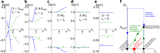
Figure S1: Adiabatic deformation of the Dirac superconducting state into a trivial material. Panels a) - e): Bogoliubov spectra keeping the $j_{z}=\pm 3/2$ and $p$ bands of Fig. 1 of the main text (energy relative to the Fermi level). The choice of parameters $t_{z},|\Delta|$ is presented in the inset. f) Contour integration entering $N(k_{z})$. Our calculation demonstrates the $N(k_{z})=-\nu_{v}\sigma_{xy,\pm}(R=0)$ using the blue dashed contour. Since the only singularity of the spectrum resides at $(t_{z},|\Delta|)=(t_{c},0)$, we conclude that the blue integration contour may be deformed into the green solid integration contour without changing the final result.

IV Quasiclassical calculation

Here, we derive our results using the method summarized in Chapter 23.2 of Ref Volovik (2003) of the main text (i.e. a quasiclassical derivation of solutions). Again, we concentrate on a given Weyl sector with normal state Hamiltonian $H_{\textbf{{p}}}=v(p_{x}\sigma_{x}+p_{y}\sigma_{y}+p_{z}(k_{z})\sigma_{z})+M(p_{z})$ (near the Weyl node $p_{z}$ is an odd function of $k_{z}$). We denote $(p_{x},p_{y})=p_{\perp}(\cos(\theta),\sin(\theta));(x,y)=\rho(\cos(\phi),\sin(\phi))$, and follow Ref. Volovik (2003) by transforming spatial coordinates to $s=\rho\cos(\phi-\theta)$ (position along a quasiparticle trajectory) and $b=\rho\sin(\phi-\theta)$ (impact parameter). We project the Hamiltonian onto the conduction band, and expand $\braket{u_{\textbf{{p}}}}{\Delta(\textbf{{r}})}{u_{\textbf{{p}}}}\simeq\Delta(\textbf{{r}})+\nabla_{\textbf{{r}}}\Delta(\textbf{{r}})\cdot(i\nabla_{\textbf{{p}}_{\perp}}+\bm{\mathcal{A}})$ (in this Section we suppress indices $\xi$ and $\pm$). We exploit that $b$ is conserved (we here consider only the lowest energy state $b=0$). In this notation we obtain

$$\mathcal{H}=\left(\begin{array}[]{cc}-iv({p_{\perp}})\partial_{s}&e^{i\theta}\left[|\Delta|\text{sgn}(s)+|\Delta|^{\prime}(i\partial_{p_{\perp}}+\mathcal{A}_{\hat{p}_{\perp}})+i\frac{|\Delta|}{{p_{\perp}}|s|}(i\partial_{\theta}+{p_{\perp}}\mathcal{A}_{\theta})\right]\\ e^{-i\theta}\left[|\Delta|\text{sgn}(s)+|\Delta|^{\prime}(i\partial_{p_{\perp}}+\mathcal{A}_{\hat{p}_{\perp}})-i\frac{|\Delta|}{{p_{\perp}}|s|}(i\partial_{\theta}+{p_{\perp}}\mathcal{A}_{\theta})\right]&iv({p_{\perp}})\partial_{s}\end{array}\right).$$ (S101)

The velocity is $v=v({p_{\perp}})=\partial\epsilon({p_{\perp}},p_{z})/\partial{p_{\perp}}$ and we suppressed the spatial dependence $|\Delta|=|\Delta(s)|$. Contrary to topologically trivial systems, $\Omega_{z}=-p_{z}/[2\sqrt{p_{z}^{2}+p_{\perp}^{2}}^{3}]$ (for $\mu>0$) does not vanish. We henceforth project to the Fermi surface $p_{\perp}\rightarrow\sqrt{p_{F}^{2}-p_{z}^{2}}\equiv q$ and we choose radial gauge, in which $\bm{\mathcal{A}}=\mathcal{A}_{\hat{p}_{\perp}}(\cos(\theta),\sin(\theta))+\mathcal{A}_{\theta}(-\sin(\theta),\cos(\theta))$ with $\mathcal{A}_{\hat{p}_{\perp}}=0$ and

$$\mathcal{A}_{\theta}(p_{\perp})=-\frac{\text{sgn}(p_{z})}{2\sqrt{p_{\perp}^{2}+p_{z}^{2}}}\frac{p_{\perp}}{\sqrt{p_{\perp}^{2}+p_{z}^{2}}+|p_{z}|}\simeq-\frac{\text{sgn}(p_{z})}{2q}\frac{1-p_{z}^{2}/p_{F}^{2}}{1+|p_{z}|/p_{F}}.$$ (S102)

Using the standard unitary transformation $e^{i\theta\tau_{z}/2}$ we obtain in close analogy to Ref. Volovik (2003)

$$\tilde{\mathcal{H}}=\left(\begin{array}[]{cc}-iv\partial_{s}&|\Delta(s)|\text{sgn}(s)+i\frac{|\Delta|}{q|s|}\left(i\partial_{\theta}-\frac{1}{2}+q\mathcal{A}_{\theta}(q)\right)\\ |\Delta(s)|\text{sgn}(s)-i\frac{|\Delta|}{q|s|}\left(i\partial_{\theta}+\frac{1}{2}+q\mathcal{A}_{\theta}(q)\right)&iv\partial_{s}\end{array}\right).$$ (S103)

In view of the hierarchy of scales $q|s|\sim\sqrt{p_{F}^{2}-p_{z}^{2}}\xi\gg 1$ we follow Eq. (23.16) of Volovik (2003) in omitting the second term of the off-diagonal elements. This leads to standard bound states in the vortex core. The perturbative inclusion of terms order $\omega_{0}\sim\Delta/(q\xi)$ implies a low energy Hamiltonian $H=\omega_{0}[Q-q\mathcal{A}_{\theta}]$ with $Q=-i\partial_{\theta}$ the angular momentum operator with usual Caroli-deGennes-Matricon quantization $Q=n+1/2$, cf. Eq. (23.23) of Volovik (2003). The gauge-symmetry enforced shift $q\mathcal{A}_{\theta}$ also follows directly from Eq. (S103). Since $q\mathcal{A}_{\theta}\simeq-\text{sgn}(p_{z})/2-p_{z}/(2p_{F})$ near $p_{z}=0$ we readily find chiral, dispersive zero modes at the projection of the Weyl node with velocity $|\Delta|/(p_{F}^{2}\xi)\sim v|\Delta^{2}|/\mu^{2}$. The inclusion of the second helical sector then implies two counterpropagating helical Majorana modes in accordance with the quantum mechanical calculation exposed above.

IV.1 Comparison to ³He-A and ³He-B

Using the technique employed in this section, one may readily compare to other systems studied with the same technique Volovik2011 ; Volovik (2003). (1) Trivial s-wave superfluids: In view of the trivial normal state band structure, $q\mathcal{A}_{\theta}$ is absent and the spectrum is gapped, $E=\omega_{0}(n+1/2)$. (2) Two-dimensional $p+ip$ superconductor $H=(\textbf{{p}}^{2}/2m-\mu)\tau_{z}+\Delta(p_{x}\tau_{x}+p_{y}\tau_{y})$: The trivial normal state Hamiltonian again implies $q\mathcal{A}_{\theta}=0$. However, the winding of the gap function in momentum space adds an additional shift of 1/2 in the low energy Hamiltonian $H=\omega_{0}[Q-1/2]$, which implies a gapless spectrum $E=\omega_{0}n$ (the $n=0$ state is usually called Majorana mode). (3) Vortex-disgyration ($\mathbb{Z}_{2}$ vortex) in ³He-A: For each spin $\sigma=\pm 1$, this phase can be described by $H=(\textbf{{p}}^{2}/2m-\mu)\tau_{z}+\sigma\Delta(p_{x}\tau_{x}+p_{y}\tau_{y})$. Therefore, the conclusions of point (2) imply a non-dispersive, doubly degenerate flat band of Majoranas in a finite interval of $p_{z}$, as long as spin components do not mix. (4) Symmetric vortex in ³He-B, where $H=(\textbf{{p}}^{2}/2m-\mu)\tau_{z}+\Delta\tau_{x}\textbf{{p}}\cdot\bm{\sigma}$: Again, $q\mathcal{A}_{\theta}=0$, and the non-trivial p dependence implies $H=\omega_{0}[Q-1/2]$. However, the spin-orbit coupled gap structure lifts the two-fold degeneracy of the one-dimensional spectrum except for helical touching points.

References

Supplementary materials for