The structure of the Mg ii broad line emitting region
in Type 1 AGNs

Abstract

We investigate the structure of the Mg ii broad line emission region in a sample of 284 Type 1 active galactic nuclei (AGNs), through comparing the kinematical parameters of the broad Mg ii and broad H$\beta$ lines. We found that the Mg ii emitting region has more complex kinematics than the H$\beta$ one. It seems that the Mg ii broad line originates from two subregions: one which contributes to the line core, which is probably virialized, and the other, ’fountain-like’ emitting region, with outflows-inflows nearly orthogonal to the disc, which become suppressed with stronger gravitational influence. This subregion mostly contributes to the emission of the Mg ii broad line wings. The kinematics of the Mg ii core emitting region is similar to that of the H$\beta$ broad line region (seems to be virialized), and therefore the Full Width at Half Maximum (FWHM) of Mg ii still can be used for the black hole (BH) mass estimation in the case where the Mg ii core component is dominant. However, one should be careful with using the Mg ii broad line for the BH mass estimation in the case of very large widths (FWHM$>$ 6000 km s^-1) and/or in the case of strong blue asymmetry.

1 Introduction

The broad emission lines (widths about several 1000 km s^-1) are one of the most important characteristics of Type 1 active galactic nuclei (AGN) spectra. They are originating in a broad line region (BLR) that is supposed to be close to the central black hole (BH) and consequently, one can assume that the BLR emission gas kinematics is virialized, i.e. it is following the gravitationally driven rotation (see e.g. Sulentic et al., 2000a; Gaskell, 2009; Netzer, 2015, etc.). The gas motion in the BLR affects the line profile (Sulentic et al., 2000a), and, in the case of Keplerian-like motion, the broad line width (Full Width at Half Maximum – FWHM) can be used for the BH mass estimation (for review see Peterson, 2014).

There are several methods for the BH mass estimation (direct and indirect, see e.g. Peterson, 2014). Among them, the reverberation method is the most frequently used one. Using reverberation, one can determine the BLR size, then assuming the virialization in the BLR and measuring the FWHM of a broad line, the BH mass can be obtained (Peterson, 1993). Reverberation was also used for establishing the relationships between the BLR size and the continuum luminosity (see e.g. Vestergaard & Peterson, 2006; Bentz et al., 2013), which is widely used for the BH mass calculations from one epoch observations.

For this purpose, there are several relationships (in different wavelength bands) between the black hole mass, continuum luminosity and broad line widths, which are defined assuming the virialization in the BLR (see e.g. Vestergaard & Peterson, 2006; Onken & Kollmeier, 2008; Vestergaard & Osmer, 2009; Wang et al., 2009; Trakhtenbrot & Netzer, 2012; Tilton & Shull, 2013; Mejía-Restrepo et al., 2016; Coatman et al., 2017; Mejía-Restrepo et al., 2018, etc.). Depending on the redshift of an AGN, there is a possibility to use different broad lines, and the most frequently used are H$\beta$, Mg ii and C iv (see Mejía-Restrepo et al., 2016).

The Mg ii relationship for the BH mass estimation is derived from the H$\beta$ relationship (see e.g. Onken & Kollmeier, 2008; Wang et al., 2009; Vestergaard & Osmer, 2009; Marziani et al., 2013a; Sulentic et al., 2014; Mejía-Restrepo et al., 2016) based on the reverberation measurements of the H$\beta$ BLR and the continuum luminosity at 5100 Å. The C iv line parameters, and consequently the estimated BH mass can be compared with those obtained from the H$\beta$ and Mg ii relationship (see e.g. Mejía-Restrepo et al., 2016; Coatman et al., 2017; Mejía-Restrepo et al., 2018). However, one of the problems of this method is the assumption that the BLR gas is virialized, particularly for the Mg ii and C iv line emitting regions (see Marziani & Sulentic, 2012; León-Tavares et al., 2013). The broad C iv and Mg ii line profiles can be affected by some other effects, as e.g. outflows (see Denney, 2012; León-Tavares et al., 2013). Therefore, there is a question of validity of using these lines and their robustness for the BH mass measurements. Since C iv and Mg ii lines are very important as BH mass estimators in high redshifted AGNs, it is of great importance to investigate the structure of their broad line emitting regions and to compare it with the H$\beta$ one for a number of AGNs. Here we will focus on the Mg ii broad line emitting region, comparing the Mg ii line shape with the H$\beta$ line profile in order to explore similarities and differences between their emitting regions.

In principle, the Mg ii 2800 Å line can be directly compared with the H$\beta$ and the consistency of the obtained BH mass using these two lines can be checked (see Wang et al., 2009; Marziani et al., 2013a, b; Mejía-Restrepo et al., 2016). However, it seems that the Mg ii emitting line region is more complex (Kovačević-Dojčinović & Popović, 2015; Jonić et al., 2016), and in some cases it can be connected with outflows (see, e.g. León-Tavares et al., 2013). There is an indication that in the case of smaller widths of Mg ii (FWHM$<$6000 km s^-1)  there is a good correlation with the H$\beta$ width, and therefore the Mg ii is equally good for BH mass estimation as H$\beta$ (Trakhtenbrot & Netzer, 2012). On the other hand, for FWHM Mg ii$>$6000 km s^-1, the difference between the FWHM of these two lines seems to be significant, and there is a question of validity of using Mg ii line for black hole mass measurements. Sulentic et al. (2000b) identified two populations of AGNs according to different spectral properties: Population A (Pop. A), with FWHM of H$\beta$ $<$ 4000 km s^-1 and Population B (Pop. B), with FWHM H$\beta$ $>$ 4000 km s^-1. Marziani et al. (2013a) found that in Pop. B, the Mg ii lines are about 20% narrower than H$\beta$ and they have more complex shape, in which one very broad, redshifted component is seen.

The aim of this work is to investigate the structure of the Mg ii broad line emitting region and to compare its kinematics with the kinematics of the broad H$\beta$ emitting region, in order to check the validity of using the Mg ii broad line as a BH mass estimator.

The paper is organized as following: In Sec. 2 we describe the sample of AGNs and give the method of analysis. In Sec.3 we explore the Mg ii line profiles in the sample of AGNs and compare the line parameters with those obtained from H$\beta$. In Sec. 4 we discuss the obtained results and possible model for the Mg ii BLR, and finally in Sec. 5 we outline our conclusions.

2 The sample and method of analysis

2.1 The sample

To investigate the assumption of virialization in the Mg ii and H$\beta$ broad line emitting regions, we used already studied sample of 293 Type 1 AGN spectra from Kovačević-Dojčinović & Popović (2015). This sample was selected from the Sloan Digital Sky Survey (SDSS), Data Release 7 and has S/N $>$ 25 (near H$\beta$ line), good pixel quality, redshift between 0.407 and 0.643 (in order to include both Mg II and H$\beta$ lines), high redshift confidence, and no absorption in the UV Fe ii lines.

Additionally, we excluded the objects with strong noise near the Mg ii line, and with absorption lines which affect the Mg ii profile. The final sample consists of 284 objects.

Figure 1: An example of the spectral decomposition to pure-host and pure-QSO contribution, using Spectral Principal Component Analysis (object: SDSS J095912.93+445059.1). Dots - observation, thin solid line - QSO, dotted line - host galaxy and thick solid line - model (QSO+host).

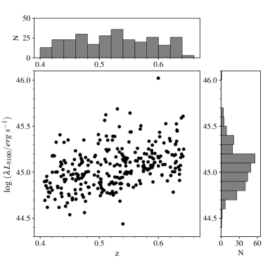
Figure 2: The AGN luminosity (after subtraction of the host galaxy contribution) vs. redshift of the sample and their distributions.

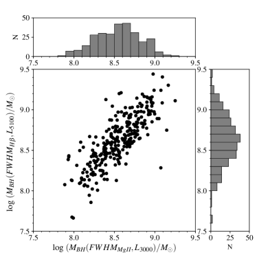
Figure 3: Estimated BH masses from the broad H$\beta$ line and continuum at 5100 Å vs. those obtained from the Mg ii broad line and continuum at 3000 Å and their distributions.

2.2 The analysis

The spectra were corrected for Galactic extinction and cosmological redshift as described in Kovačević-Dojčinović & Popović (2015). In Kovačević-Dojčinović & Popović (2015) the host galaxy contribution is was assumed to be negligible in this sample since majority of objects have high continuum luminosity (see their Fig 1). However, in order to estimate more precisely the continuum luminosity, here we applied the Spectral Principal Component Analysis method (see Connolly et al., 1995; Yip et al., 2004a, b) to subtract the host contribution (see Vanden Berk et al., 2006) and obtain the pure AGN continuum. For the subtraction of the host-galaxy contribution, we followed the procedure described in more detail in Lakićević et al. (2017). We found that in the majority of spectra the host-galaxy component is negligible (as it was assumed in Kovačević-Dojčinović & Popović, 2015). The significant host contribution was found only in 43 objects. For majority of these 43 objects, the host contribution is smaller than 15% at 5100 Å. The example of spectral decomposition to pure-host and pure-AGN contribution is shown in Fig 1. After the host galaxy subtraction, the pure QSO continuum flux is measured at 5100 Å, and continuum luminosity is calculated using the formula given in Peebles (1993), and the cosmological parameters $\Omega_{M}$=0.3, $\Omega_{\Lambda}$=0.7 and $\Omega_{k}$=0, and Hubble constant $\rm H_{0}$=70 km s^-1 Mpc^-1. The host-corrected continuum luminosity at 5100 Å vs. redshift and their distributions are shown in Fig 2.

The procedure for the fitting of the AGN spectra is given in Kovačević-Dojčinović & Popović (2015). After the continuum subtraction, we applied the multi-Gaussian emission line model, in which the complex line shapes are fitted with Gaussians of different widths, shifts and intensities, with the assumption that each Gaussian represents the emission from one emission region (see Popović et al., 2004; Kovačević et al., 2010). To reduce the number of free parameters in the fitting procedure, we assumed that the width and shift of each Gaussian are connected with the kinematical properties of the emission region where the corresponding line component arises. As e.g. the narrow H$\beta$ and [O iii] lines are assumed to be emitted from the same region, so the velocity dispersion of the Gaussian of the narrow H$\beta$ and [O iii] are assumed to be same, as well their shifts. In this way, all lines or line components, which are supposed to originate from the same emission line region, are fixed to have the same widths and shifts (see Popović et al., 2004).

For this research, it is necessary to extract the pure broad H$\beta$ and Mg ii profiles from the complex AGN spectra, which is a very difficult task, with some level of uncertainties. The biggest problem is to remove the overlapping lines, as e.g. Fe ii lines in the optical (around H$\beta$) and in the UV (around Mg ii), and the narrow component of the H$\beta$ line.

The model of the line decomposition and the procedure of the spectral fitting in optical $\lambda\lambda$ 4000-5500 Å and UV $\lambda\lambda$ 2650-3050 Å band are presented in detail in Kovačević et al. (2010), and Kovačević-Dojčinović & Popović (2015), and here we just recall the important steps for obtaining the broad H$\beta$ and Mg ii lines.

Figure 4: Panel (a): the mean (solid line) and RMS (dashed line) Mg ii profiles of 284 AGNs. Panel (b): the same for H$\beta$. Panel (c): the comparison of the H$\beta$ (solid line) and Mg ii (dashed line) mean profiles. The horizontal solid lines indicate the widths at half and 10% of the maximal intensity. Panel (d): the Mg ii broad line (dashed line) rescaled to have the same FWHM as the H$\beta$ (dotted line) and their difference (solid line).

2.2.1 The pure broad H$\beta$ profile

The broad H$\beta$ line overlaps with the numerous optical Fe ii lines, [O iii] $\lambda\lambda$ 4959, 5007 Å doublet and narrow H$\beta$ component.

In the line decomposition model, the complex optical Fe ii bumps are fitted with the Fe ii semi-empirical model presented in Kovačević et al. (2010) and Shapovalova et al. (2012). This Fe ii model enables very precise fitting of the Fe ii bumps in the 4000-5500 Å spectral range (see appendix in Kovačević et al., 2010). The Balmer lines in the range $\lambda\lambda$ 4000-5500 Å (H$\delta$, H$\gamma$ and H$\beta$) are fitted with three components - one narrow and two broad components, one which comes from the Very Broad Line Region (VBLR) and fits the line wings, and the other which comes from the Intermediate Line Region (ILR) and fits the core of the Balmer lines (see Popović et al., 2004; Bon et al., 2006; Hu et al., 2008). The widths and shifts of each line component are thus the same for all considered Balmer lines, which reduces the uncertainties in the H$\beta$ line decomposition.

In some cases, the Balmer narrow lines are very difficult to resolve from the broad line component, especially in so-called Pop. A objects (see Sulentic et al., 2000b). On the other hand, the [O iii] lines are well resolved in the majority of spectra. Therefore, the narrow Blamer lines are fixed to have the same width and shift as [O iii] lines, since we are assuming that they arise in the same Narrow Line Region (NLR), and thus have the same kinematical properties. In this way, the number of free parameters in the fitting procedure is reduced and more accurate fitting decomposition is achieved.

Nevertheless, there is still some doubt about the non-uniqueness of the H$\beta$ line decomposition to the broad and narrow component. Popović & Kovačević (2011) tested the uniqueness of the H$\beta$ decomposition with this model, and discussed it in the Appendix A (in the same paper). As it can be seen from Popović & Kovačević (2011) the method we applied can reasonable fit the narrow H$\beta$ component, and consequently the narrow H$\beta$ component can be subtracted in order to find the pure H$\beta$ broad component.

Figure 5: Panel (a): the relationship between the widths of the line measured at 10% and 50% of the maximal line intensity (FW10%M vs. FWHM). Panel (b): the relationship between the width and intrinsic shift measured at 10% of the maximal line intensity (z_10% vs. (FW10%M)²). The triangles denote the Mg ii and full circles H$\beta$ data.

2.2.2 The pure broad Mg II $\lambda$ 2800 Å profile

In the UV part of AGN spectrum, the Mg ii line is contaminated with the Balmer continuum and numerous UV Fe ii lines. In addition, the Mg ii line is a doublet with two components which overlap: $\lambda$ 2796 Å and $\lambda$ 2803 Å, that makes the extraction of the single broad profile even more complicated. The ratio of the component intensity is unknown, and it depends on the optical depth of the Mg ii emitting region. In the optically thin case, the ratio Int(Mg ii $\lambda$ 2796 Å)/Int(Mg ii $\lambda$ 2803 Å) is expected to be 2:1, while in the case of fully thermalized lines it should be 1:1 (Laor et al., 1997; Marziani et al., 2013a). For expected values of parameters in the AGN emission region (hydrogen density and ionization parameter) this ratio should be close to 1:1 (Marziani et al., 2013a). Taking into account that the doublet transition wavelength separation is $\sim$ 8 Å ($\sim$260 ${\rm kms^{-1}}$) and that the total line width is one order of magnitude larger, Mg ii can be considered as a single line. Therefore, we assumed that Mg ii profile and FWHM Mg ii are not affected by doublet separation.

Note here that some authors apply the fitting procedure of the Mg ii with broad and narrow line components (see McLure & Dunlop, 2004; Wang et al., 2009; Shen & Liu, 2012). However, the Mg ii abundance and the transition probability for the NLR conditions are too small, so the narrow Mg ii component seems to be absent or very weak and can be neglected (Wang et al., 2009; Marziani et al., 2013a; Kovačević-Dojčinović & Popović, 2015). Moreover, by visual inspection of the Mg ii lines in our sample we could not find any spectrum with the prominent narrow Mg ii line. Therefore, we neglected the Mg ii narrow line contribution to the broad Mg ii component.

For the Balmer continuum, we used the model given in Kovačević et al. (2014).

The UV Fe ii lines around the Mg ii are complex, and there are several theoretical and empirical templates of the UV Fe ii lines (see e.g. Bergeron & Kunth, 1980; Vestergaard & Wilkes, 2001; Tsuzuki et al., 2006; Bruhweiler & Verner, 2008; Kovačević-Dojčinović & Popović, 2015). We tested several templates and found that (see more details in Appendix A): (i) the theoretical templates could not fit well the UV Fe ii lines; (ii) the empirical templates are based on I Zw 1 Fe ii emission, which is narrow-line Seyfert 1 galaxy, and one cannot expect that in the case of the broad line AGNs the ratio between the UV Fe ii multiplets is the same as in the case of I Zw 1 (as in the case of the optical Fe ii lines, see Kovačević et al., 2010; Popović & Kovačević, 2011).

To solve this problem, we developed a semi-empirical model of the UV Fe ii lines based on the model given in Kovačević-Dojčinović & Popović (2015), where the Fe ii multiplet intensities are free parameters, but the line ratios within one Fe ii multiplet are fixed, taking that within a multiplet the intensity ratio of two lines is:

$${I_{1}\over I_{2}}$=${[{\lambda_{2}\over\lambda_{1}}]}^{3}\cdot\frac{f_{1}}{f_{2}}\cdot{g_{1}\over g_{2}}\cdot e^{-[E1-E2]/kT}$$ (1)

where $I_{1}$ and $I_{2}$ are intensities of the lines with the same lower level of transition, $\lambda_{1}$ and $\lambda_{2}$ are line wavelengths, $g_{1}$ and $g_{2}$ are corresponding statistical weights of the upper levels, and $f_{1}$ and $f_{2}$ are oscillator strengths, $E_{1}$ and $E_{2}$ are energies of the upper level of transitions, $k$ is Boltzmann constant, and $T$ is the excitation temperature.

Taking that in our case the $\lambda_{2}\sim\lambda_{1}$, and $E_{1}\sim E_{2}$, an approximation can be used as:

$${I_{1}\over I_{2}}\sim{f_{1}\over f_{2}}\cdot{g_{1}\over g_{2}}$$ (2)

as in the paper of Kovačević-Dojčinović & Popović (2015). Here we use Eq. (1), to calculate the values of the line ratios within multiplets in Appendix A. In Appendix A we give a detailed discussion about the UV Fe ii semi-empirical model as well as comparison of this model with theoretical and empirical templates. Additionally, using our model we calculated a grid of the UV Fe ii templates in the 2650-3050 Å range with different FWHM and shifts of the UV Fe ii lines..

The Mg ii line was fitted with two broad Gaussians: one which fits the core, and one which fits the line wings. These two broad Gaussians reproduce well the Mg ii line profiles in our sample.

2.2.3 Measuring the broad line parameters and black hole masses

The Mg ii and H$\beta$ broad line shapes have been reproduced from the best fit (from two Gaussians), then normalized to one, and FWHM and Full Width at 10% of the Maximal Intensity (FW10%M) were measured. The corresponding intrinsic shifts (z_50% and z_10%) are measured as well, as a centroid shift with respect to the broad line peak at 50% and 10% of Maximal Intensity, respectively (see Jonić et al., 2016).

The black holes masses (M_BH) are estimated from relationships of Vestergaard & Peterson (2006) which uses the H$\beta$ parameters, and Vestergaard & Osmer (2009) which uses the parameters of Mg ii line. In Fig. 3 we show the BH masses derived from H$\beta$ vs. those derived from Mg ii line and their distributions. As it can be seen in Fig. 3, there is strong correlation between the BH masses derived from these two lines, and their distributions are very similar.

2.2.4 The mean and RMS line profiles

To explore the Mg ii and H$\beta$ line profiles, we found the mean profiles of the normalized H$\beta$ and Mg ii lines from the sample and the root-mean-square – RMS which indicates the difference in the line profiles (see Fig. 4ab). Comparing the mean Mg ii and H$\beta$ line profiles we found that the line cores are very similar, and that the difference is seen in the line wings (Fig. 4c).

The slight difference in the line cores is caused by a smaller FWHM Mg ii. Therefore, to subtract two mean profiles, we first rescaled Mg ii to have the same FWHM as H$\beta$ for each AGN (Fig. 4d). As the result of subtraction, a double peaked feature appeared (see solid line in Fig. 4d). It seems that there is an extra emission in the far (blue and red) Mg ii wings compared to the H$\beta$ ones, with a bigger difference in the blue wings (see Fig. 4d).

2.3 Connections between the Mg ii and H$\beta$ line widths/shifts – virialization assumption

To test the virialization in the Mg ii and H$\beta$ line emitting regions we used the line parameters: intrinsic shifts and FWHMs of all AGNs in the sample. The FWHM can be related with the line dispersion sigma, which is the second moment or variance of the velocity distribution (as e.g. is the case for Gaussian-like profile). In particular case where we assume a Keplerian-like motion, the FWHM is directly connected with the velocity and with the emissivity weighted radius $R_{\rm FWHM}$, so the mass of the central black hole can be estimated from (see e.g. Peterson, 2014):

$$M_{\rm BH}\sim{\rm FWHM}^{2}\cdot R_{\rm FWHM}$$ (3)

Therefore, in the virialization assumption, the rotating velocity is strongly connected with the FWHM.

Assuming the Keplerian motion, one can write the following:

$$M_{\rm BH}$=$R_{\rm BLR}\cdot v^{2}/G$$ (4)

where $R_{\rm BLR}$ is the size of the rotating BLR and $v$ is the velocity of the rotation.

Concerning the line intrinsic shift (asymmetry), it can be caused due to a number of effects, but in the case of full virialization, one can expect the connection between the intrinsic line shift and FWHM.

Namely, if we take that the BH mass can be measured using the gravitational shift ($z_{g}$) as (Liu et al., 2017):

$$M_{\rm BH}\sim R_{\rm BLR}\cdot z_{g}\sim R_{\rm BLR}{\rm FWHM}^{2},$$ (5)

this indicates that a good correlation should be present between $z_{g}$ and ${\rm FWHM}^{2}$. Since we measured the intrinsic shift at FWHM ($z_{50\%}$) and FW10%M ($z_{10\%}$), in the case of virialization in the total line we expect:

$$z_{50\%}\sim{\rm FWHM}^{2},\ \ \ \ \ \ \ \ \ z_{10\%}\sim{\rm FW10\%M}^{2}$$ (6)

where $z_{50\%}$ and $z_{10\%}$ are measured intrinsic shifts at FWHM and FW10%M (see Jonić et al., 2016).

Using Eq. (6) we explored the virialization in the Mg ii and H$\beta$ emitting regions.

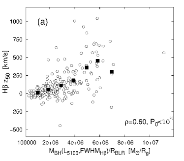
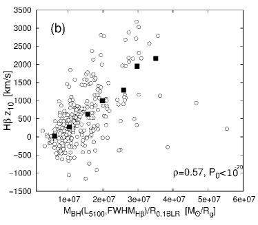
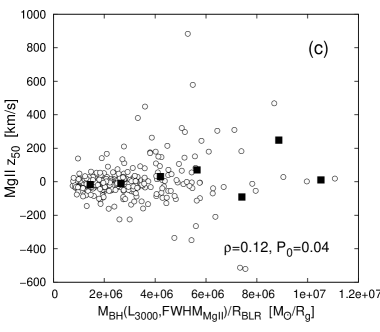
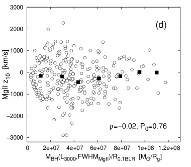
Figure 6: The intrinsic shifts at 50% and 10% of the maximal line intensity as the function of $M_{\rm BH}/R$ ratio for H$\beta$ (a, b) and Mg ii (c, d). The binned values are denoted with black squares.

3 Results

In order to investigate similarities and differences between the H$\beta$ and Mg ii emitting regions, we compared the mean and RMS line profiles of these broad lines (see §2.2.4).

As it can be seen in Fig. 4ab the mean Mg ii broad line has Lorentzian-like profile, while the mean broad H$\beta$ mostly has a Gaussian-like profile. The mean Mg ii broad line profile (normalized to one) is similar to H$\beta$ in the line core (with slightly smaller FWHM), while in the line wings there is a large difference. The Mg ii has more extensive line wings (see Fig. 4cd), and specially, the blue wing tends to be more intensive than the red in comparison with the H$\beta$ ones.

The mean and RMS line profiles are taken from a sample that has the AGN luminosity spanning an order of magnitude from $\log(\lambda L_{5100})\sim$ 44.5 to $\log(\lambda L_{5100})\sim$ 45.5 (see Fig. 2) and different black hole masses (see Fig. 3). Therefore, some other effects may affect the broad emission line features such as a flux excess in the red or/and blue side of line profile as e.g. photoionization effects in the BLR, geometry and dynamics of the BLR, etc. However, in this paper we are a priori assuming the virialization in the Mg ii and H$\beta$ emitting regions. Therefore, the FWHM should depend on the BH mass ($M_{\rm BH}$), and BLR radius ($R_{\rm FWHM}$), i.e. ${\rm FWHM}\sim\sqrt{M_{\rm BH}/R_{\rm FWHM}}$.

Taking a sample with different BH masses, one can expect that the RMS of normalized line profiles should have maxima around the velocities that correspond to the $\lambda_{1}$=$\lambda_{0}-{\rm FWHM}/2$ and $\lambda_{2}$=$\lambda_{0}+{\rm FWHM}/2$ (since the line maximum is normalized to one). Fig. 4ab shows that the RMS has two maxima around $\lambda_{0}\pm{\rm FWHM}/2$ in the case of both lines. Additionally, if both broad lines originate from the region with similar kinematics, one can expect that the mean Mg ii and H$\beta$ broad lines should have similar profiles, as it is the case with their line cores (see Fig. 4cd). It is clearly seen that there is a large difference in the line wings, where Mg ii shows broader and more intensive line wings.

On the other hand, in the case that another geometry dominates the BLR, as e.g. inflow/outflow, one can expect that the RMS would have strong asymmetry (and peaks) in the far blue or red line wings. In other words, the mean and RMS profiles of the sample AGNs with different masses and BLR properties, can give some indications about the difference in the BLR geometry, especially if we compare mean profiles of two different lines from the sample. Note here that in the case where the kinematics plays an important role in the line shapes, one can expect that in one spectrum the normalized Mg ii and H$\beta$ broad line profiles should have similar (almost the same) shape.

The Mg ii RMS has two peaks (at $\sim$-1720 km s^-1 and $\sim$+1800 km s^-1) and is nearly symmetric, while the H$\beta$ RMS has red asymmetry (two peaks at $\sim$-1860 km s^-1 and $\sim$+2080 km s^-1). The distance between the RMS peaks in the both lines is very close to the FWHM of their mean profiles.

3.1 The Mg ii and H$\beta$ BLR kinematics

Since the FWHM of the broad H$\beta$ and Mg ii lines are in a good correlation (see e.g. Kovačević-Dojčinović & Popović, 2015), one can expect that their other parameters are also well correlated. However, the correlation is absent in the case of FW10%M between these two lines (see e.g. Jonić et al., 2016). Here we explored correlation between kinematical parameters of Mg II and H$\beta$ in more detail (see Fig. 5).

We compared the FW10%M vs. FWHM for both lines (Fig. 5a). The H$\beta$ line parameters are in good correlation: $\rho$=0.82, $P_{0}<$10^-20, where $\rho$ is Spearman correlation coefficient and $P_{0}$ is P-value of the null-hypothesis. In the case of the Mg ii line the correlation between these parameters is weaker ($\rho$=0.42, $P_{0}$=10^-13).

As mentioned before, if virialization is present in an emitting region, one can expect that the intrinsic shift will be in correlation with the corresponding width (see Eq. 6). In Fig. 5b we showed the correlations between the intrinsic shifts and widths at 10% of the line maximum. The expected correlation is present in the case of H$\beta$ ($\rho$=0.57, $P_{0}<$10^-20), but in the case of Mg ii there is no trend ($\rho$=-0.02, $P_{0}$=0.71). The big scattering of the points is present, showing randomly strong blue and red shifts in the wings. This indicates that the Mg ii wings probably originate in a region that is more connected with outflows/inflows than with the virial motion of the gas in an accretion disc.

We should note that the relationship between the line profile width and centroid wavelength shift can be questioned, since the gravitational redshift is typically assumed to have a minimal effect on the line profile. To do an additional test of the connection between the intrinsic shift and the gravitational redshift, we explored the intrinsic shift as a function of the $M_{\rm BH}/R_{\rm BLR}$ ratio (see Eq. 5), using the BLR size from the $R-L$ relation (given in Bentz et al., 2013) and the single-epoch BH mass.

For the intrinsic shift at 10% of the maximal intensity we rescaled the $R_{\rm BLR}$ as:

$$R_{\rm 0.1BLR}$=$R_{\rm BLR}\cdot\Bigg{(}\frac{{\rm FWHM}}{{\rm FW10\%M}}\Bigg{)}^{2}.$$ (7)

In Fig. 6 we plot the intrinsic shift measured at FWHM ($z_{50\%}$) and at FW10%M ($z_{10\%}$) as a function of the $M_{\rm BH}/R_{\rm BLR}$ for H$\beta$ (Figs. 6ab) and Mg ii (Figs. 6cd). Also we show the binned values (black squares) in order to trace a trend between the intrinsic shift and the $M_{\rm BH}/R_{\rm BLR}$ ratio. Figs. 6ab show that the intrinsic shifts follow the expected correlation with the $M_{\rm BH}/R_{\rm BLR}$ for H$\beta$. In the case of the intrinsic shift at half of the maximal intensity for Mg ii, there is some indication of a weak trend with the $M_{\rm BH}/R_{\rm BLR}$ only for $z_{50\%}>$0 (Fig. 6c), but the intrinsic shift of Mg ii wings shows no correlation with the $M_{\rm BH}/R_{\rm BLR}$ (Fig. 6d). This implies that there is no virialization in the Mg ii wings. The values of the intrinsic shift in Mg ii are in the range from -3000 km s^-1 to +2000 km s^-1 (see Fig. 6d) which indicates high outflows/inflows, with similar probability. However, as $M_{\rm BH}/R_{\rm BLR}$ increases, the range of intrinsic shift gets smaller (between $\pm$1000 km s^-1), i.e. this kind of motion is with smaller velocity. These results indicate some kind of ’fountain-like’ motion that contributes to the extensive Mg ii line wings, which becomes suppressed with stronger gravitational influence.

Additionally, we investigated the influence of the Eddington ratio to the gas velocities in the ’fountain-like’ region. Therefore, we calculated the $L_{5100}$/$M_{\rm BH}\big{(}H\beta\big{)}$ ratio (which is proportional to the Eddington ratio) for a subsample of 52 objects with the luminosities in the narrow range of 45.1$<\log(\lambda L_{5100})<$45.2, and we tested if there is a correlation with $z_{10\%}$, which is probably proportional to the ’fountain-like’ region velocities. We found that the absolute value of $z_{10\%}$ (|$z_{10\%}$|) has weak correlation with $log\big{(}L_{5100}$/$M_{\rm BH}\big{(}H\beta\big{)}\big{)}$ ($\rho$=0.34, $P_{0}$=0.01), i.e the inflow/outflow velocities increase as Eddington ratio increases.

Figure 7: The mean (solid tick line) and the RMS (dashed tick line) Mg ii broad line profiles for sub-samples of AGNs, for which Mg ii: (a) has red asymmetry (29 AGNs with $z_{50\%}>100$km s^-1); (b) is almost symmetric (231 AGNs with $z_{50\%}$ between $\pm 100$km s^-1); and (c) has blue asymmetry (24 AGN with $z_{50\%}<-100$km s^-1). The Mg II asymmetry is measured at FWHM. The corresponding mean H$\beta$ and RMS profiles are shown with thin solid and dashed lines, respectively.

Figure 8: Comparison between the mean Mg ii and H$\beta$ broad line profiles and their difference (dashed line) for the samples of (a) 149 Pop. A objects (FWHM H$\beta<$4000km s^-1) and (b) 135 Pop. B objects (FWHM H$\beta>$4000km s^-1).

4 Discussion

4.1 Similarities and differences between Mg ii and H$\beta$ emission line profiles

First of all, let us give some general facts about the Mg ii and H$\beta$ line profiles:

• The core and FWHM of the mean profiles of Mg ii and H$\beta$ seem to be very similar, while the difference is bigger in the line wings. The Mg ii line has more Lorentzian-like, and the H$\beta$ has Gaussian-like profile.

• The H$\beta$ line shows virialization in the whole profile, i.e. the relationship between the kinematical parameters (widths and intrinsic shifts) obtained from the H$\beta$ BLR nearly follows those expected in case of the pure Keplerian motion. On the other hand, the Mg ii BLR does not follow this motion.

• It seems that Mg ii shows virialization in the line core, while another effect contributes to the line wings, making them very extensive.

There is a question how much an emitting region with inflows and/or outflows contributes to the total Mg ii emission. At least in the wings, we can expect the contribution of the emitting region with some kind of vertical (to the disc plane) motion.

Since the line profiles can indicate the inflow (red asymmetry) or outflow (blue asymmetry), we divided the sample into three subsamples according to the Mg ii asymmetry (i.e. z_50% measured at FWHM). The first subsample contains AGNs with the Mg ii blue asymmetry ($z_{50\%}<-100$ km s^-1), the second with the red one ($z_{50\%}>100$ km s^-1), and the third contains the AGNs with the symmetric Mg ii profile (intrinsic shift, $z_{50\%}$, between these two values: $-100<z_{50\%}<+100$). We found that most of AGNs (231) have almost symmetric Mg ii mean profile, showing extended wings in Mg ii compared to H$\beta$, and a big difference in the line wings of these two lines (see Fig. 7b). The red asymmetry is present in 29 AGNs, and as it can be seen in Fig. 7a, the mean line profiles of Mg ii and H$\beta$ are very similar (almost the same) for these objects. Finally, we found 24 AGNs with the significant blue asymmetry, and also with a big difference between the mean Mg ii and H$\beta$ line profiles (see Fig. 7c).

Comparing the mean H$\beta$ and Mg ii line profiles and their RMSs (Fig. 7), one can conclude that in the case of the red asymmetry and symmetric Mg ii profiles, the FWHM and RMSs are similar for both lines in the most of cases (see Fig. 7ab), and the Mg ii line seems to be a good estimator of the central BH mass. In the case of the strong blue Mg ii asymmetry, the mean profiles of Mg ii and H$\beta$ are quite different, and the Mg ii line perhaps is not appropriate for BH mass estimation. However, we should note that we have statistically small samples of objects with strong blue and red asymmetry, so the result may be influenced by outliers.

Let us here also recall the results obtained in Marziani et al. (2013a, b). They found a difference in the line profiles of Mg ii and H$\beta$ for Pop. A and Pop. B objects (see the definition of Pop. A/Pop. B in Sec. 1). The red asymmetry was observed in the Pop. B objects in both broad lines (Mg ii and H$\beta$) and they supposed that it may indicate an inflow in the BLR. Pop. A objects have more symmetric line profiles, but the blue-shift of Mg ii relative to H$\beta$ indicates an outflow (Marziani et al., 2013b). Therefore, one can conclude that the Mg ii line profiles in AGN show both outflows (Pop. A objects) and inflows (Pop. B objects).

We also compared the line profiles of Pop. A and Pop. B objects in our sample. We found that 149 objects from the sample are Pop. A, with the FWHM of H$\beta$ smaller than 4000 km s^-1, and 135 objects are Pop. B. The comparison of the Mg ii and the H$\beta$ mean line profiles for both populations is presented in Fig. 8. It can be seen that the Mg ii wings are more extensive than H$\beta$ wings, and that H$\beta$ is slightly broader than Mg ii in both populations (as it was noted in Marziani et al., 2013a, b). Also, the mean H$\beta$ and Mg ii line profiles are different in these two populations. In Pop. A, the mean Mg ii profile is Lorenzian-like, and it shows blue asymmetry in wings (velocities at 10% of line intensity: -5780 km s^-1 to +5100 km s^-1, see Fig. 8a), while the mean H$\beta$ has red asymmetry (velocities at 10% of line intensity: -3990 km s^-1 to +4590 km s^-1). However, if measured at 50% of line intensity, both lines are nearly symmetric (Mg ii: -1380 km s^-1 to +1350 km s^-1, H$\beta$: -1520 km s^-1 to +1560 km s^-1). In Pop. B, the red asymmetry in the mean H$\beta$ line profile is much stronger compared to Pop. A (velocities at 10% of line intensity: -5110 km s^-1 to +6740 km s^-1, and at 50% of line intensity: -2410 km s^-1 to +2750 km s^-1), while the Mg ii mean profile is almost symmetric with a slight asymmetry measured at 10% of line intensity in the blue wing (-6620 km s^-1) compared to the red wing (+6470 km s^-1), and at FWHM the profile is symmetric (with FWHM/2 $\sim\pm$ 1960 km s^-1).

Similarly as Marziani et al. (2013b), we found that the mean H$\beta$ and Mg ii profiles are nearly symmetric in Pop. A (measured at FWHM), and that the mean H$\beta$ profile has red asymmetry in Pop. B. However, in difference with Marziani et al. (2013b), we found that emission in far wings of Mg ii is present (that is assumed as an iron contribution in Marziani et al., 2013b), and we found no red asymmetry in Pop. B Mg ii mean profile. Note here that in this sample, for the Pop. B objects, the FWHM Mg ii is mostly in the range of 4000 km s${}^{-1}<$ FWHM Mg ii $<$ 6000 km s^-1. There are only three objects with FWHM Mg ii $>$ 6000 km s^-1 (see Fig 5a), while in the sample of Marziani et al. (2013a, b), there are dozens of objects like this (see Fig 8 in Marziani et al., 2013a). For the mean Mg ii profile of these three objects with FWHM Mg ii $>$ 6000 km s^-1, we found the red asymmetry in the line wings (see Sec 4.2), as Marziani et al. (2013a) found for Pop. B in their sample.

The possible Fe ii emission contribution in the red and blue wings of the Mg ii and H$\beta$ is discussed in Appendix A of this paper.

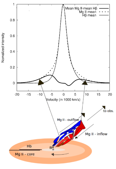
Figure 9: Upper panel shows the mean Mg ii (dashed line) fitted with the H$\beta$ mean profile (solid thin line). Their difference is shown below as double-peaked feature (solid tick line). Bottom panel presents a simple scheme of Mg ii and H$\beta$ emitting regions in AGNs, where the flow orthogonal to the disc is caused by outflows and inflows. This motion contributes to the Mg ii line wings (see upper panel). The BLR with disc-like rotation contributes to the Mg ii line core and mostly to the total H$\beta$ broad line.

4.2 Mg ii emitting region

Comparing the mean Mg ii and H$\beta$ line profiles in the total sample and five sub-samples (see Fig. 4cd and Figs. 7 and 8), the large difference seems to be visible only in wings. The question is what can cause the difference only in the line wings? We found that the intrinsic shift in the Mg ii wings can be red or blue and that it is not in correlation with the $M_{\rm BH}/R_{\rm BLR}$ ratio (see Fig. 6d), which indicates that both, inflows and outflows could be present in the Mg ii emitting region. To discuss a model for the Mg ii emitting region, let us recall some results from the laboratory plasma investigations. As it was shown in Kuraica et al. (2009, see Fig. 6 in their paper), the kinematics can affect the line profile in the case of ’fountain-like’ motion with approaching and receding velocities, that in combination with the Doppler broadening can produce slightly asymmetric Lorentzian-like profiles. Also, recently Czerny et al. (2017) showed that a flow with an orthogonal motion to the disc plane can produce Lorentzian-like profiles. The similar results, with Lorentzian like profile was obtained by Kollatschny & Zetzl (2013), considering some type of turbulent velocities in the model (vertical to the BLR rotation).

In Fig. 9 (upper panel) we fitted the Mg ii mean profile (dashed line) with the H$\beta$ one (solid line), and subtracted the best fit of H$\beta$ from Mg ii (thick double-peaked feature shown below). As expected, there is a double peaked structure emerging after the subtraction, showing the maxima at $\sim\pm 7000$ km s^-1. If there are some kind of outflows-inflows they should have high velocities, i.e. probably the outflows-inflows originate very close to the central BH. One can also consider that this extra-emission may come from the fast motion of the material in the accretion disc, that is very close to the central BH. However, in that case we expect to have boosted blue wing and large red wing that is typical for the relativistic disc (see e.g. the complex profile of NGC 3516, Figs. 7-10 in Popović et al., 2002), which is not the case here (see Fig. 9). Therefore, we excluded this scenario.

Taking into account the discussion above, we propose the following scenario for the Mg ii line origin (as it is shown in the simple scheme in Fig. 9, bottom):

The line core is originating from the virialized disc-like BLR (represented as a disc in Fig. 9-bottom panel), that may be at slightly larger radius than the H$\beta$ emission region (Mg ii shows a slightly narrower FWHM than H$\beta$). In the case where the emission from this region is dominant, the FWHM of Mg ii represents the velocity of the emission gas rotation due to gravitational force, and the line can be used as very good BH mass estimator, as it is noted in Trakhtenbrot & Netzer (2012). However, where the ’fountain-like’ region is dominant (shown as outflows-inflows in Fig. 9-bottom), one can expect a broader Mg ii line, and in that case, the virialization in the FWHM probably is not present, and therefore Mg ii might not be suitable for the BH mass estimation (León-Tavares et al., 2013). This is in agreement with results obtained by Trakhtenbrot & Netzer (2012), who found that the Mg ii can be used as a good BH mass estimator in the case of FWHM$<$6000 km s^-1.

As mentioned above, we found only 3 AGNs with Mg ii FWHM larger than 6000 km s^-1, for which we compared the mean H$\beta$ and Mg ii line profiles (see Fig. 10). As it can be seen, there is a difference between the mean H$\beta$ and Mg ii lines and their RMS profiles. The Mg ii mean profile shows red asymmetry measured at 10% of line intensity (-7300 km s^-1 to +7760 km s^-1) and it is nearly symmetric at FWHM (-3240 km s^-1 to +3270 km s^-1), while the H$\beta$ mean profile shows strong red asymmetry measured at both 10% (-5940 km s^-1 to +8680 km s^-1) and 50% of line intensity (-3090 km s^-1 to +3970 km s^-1). Additionally, the differences (RMS) in far wings of the mean Mg ii are without peaks which are usually seen near $\lambda_{0}\pm$FWHM/2 in the RMS of H$\beta$.

Therefore, despite our limited number of objects with Mg ii FWHM$>$6000, our analysis of these objects is in agreement with previous results. However, since our sample has no statistically significant number of AGNs with very broad Mg ii lines, we could not find the strict constraint in the Mg ii line parameters (width or asymmetry) which would indicate if Mg ii is suitable (or not suitable) for BH mass estimation (see Appendix B).

Figure 10: Mean line profiles of Mg ii (tick line), and H$\beta$ (thin line) for 3 AGNs with FWHM Mg ii $>$ 6000 km s^-1. Corresponding RMS profiles are denoted with tick dashed line (for Mg ii) and thin dashed line (for H$\beta$). The vertical lines show positions of $\lambda_{0}\pm$FWHM/2, where it is expected to have RMS peaks due to the difference in BH masses.

5 Conclusions

Here we explored the structure of the Mg ii line emitting region in a sample of 284 type 1 AGNs, by comparing the Mg ii line parameters with the H$\beta$ ones. We investigated measured line properties and tried to give the possible model of the broad Mg ii emitting region.

From our analysis we can conclude the following:

• The mean Mg ii line profile has a slightly asymmetric Lorentzian-like profile, and very broad line wings. The shape of the mean Mg ii line profile and correlation between the line parameters indicate that there are two Mg II emitting regions: the one similar to the H$\beta$ emitting region that is probably virialized (contributes to the line core), and the second emission region that seems to be ’fountain-like’. In order to explain the broad blue and red wings, the ’fountain-like’ emission region should have both – inflows and outflows, with high velocity components orthogonal to the disc, which become suppressed with stronger gravitational influence.

• If the virialized region mostly contributes to the Mg ii line flux, the Mg ii FWHM should be comparable with the H$\beta$ one, and it can be used for BH mass estimation. However, if the contribution of the ’fountain-like’ region is more dominant, one can expect to have broader Mg ii lines, with extensive wings. This is especially seen in the case of very broad Mg ii with FWHM $>$ 6000 km s^-1, or in the case of the Mg ii with a strong blue asymmetry; in both cases we found that the FWHM probably does not represent the rotational motion of the emitting gas in the central BH gravitational field. Therefore, one should be careful when using extremely broad or blue asymmetric Mg ii line for BH mass estimation.

6 Acknowledgments

This work is a part of the project (176001) ”Astrophysical Spectroscopy of Extragalactic Objects” supported by the Ministry of Education, Science and Technological Development of Serbia. We thank to the referee for very useful comments which significantly improved the paper.

Appendix A The UV and optical Fe II line subtraction

There are different UV and optical Fe ii templates presented in the literature (see e.g. Boroson & Green, 1992; Vestergaard & Wilkes, 2001; Tsuzuki et al., 2006; Bruhweiler & Verner, 2008; Kovačević et al., 2010; Kovačević-Dojčinović & Popović, 2015; Mejía-Restrepo et al., 2016, etc.) which are used to account for the iron emission contribution to the H$\beta$ and Mg ii line profiles. For the subtraction of the optical Fe ii lines around H$\beta$ we used the model given in Kovačević et al. (2010). The differences between this Fe ii model and models given in Dong et al. (2008) and Bruhweiler & Verner (2008) are explored and analysed in Appendix B of Kovačević et al. (2010), where it is demonstrated that this template can well reproduce the Fe ii optical emission around the H$\beta$ line. Barth et al. (2015) compared this template with the ones of Boroson & Green (1992) and Veŕon-Cetty et al. (2004), and they found that it returns the best $\chi^{2}$ values. Since the optical Fe ii model given in Kovačević et al. (2010) is analysed in number of papers, we will not consider it here in more detail.

For subtraction of the UV Fe ii lines we used the UV Fe ii model given in Kovačević-Dojčinović & Popović (2015), which has been improved for the purpose of this investigation. Therefore, here we give more details about improved version of that model.

A.1 The improved UV Fe ii model in the $\lambda\lambda=$2650-3050 Å wavelength range

In order to test the model of UV Fe ii given in Kovačević-Dojčinović & Popović (2015), we fitted set of spectra with different width of emission lines. We found that in the case of type 1 AGNs, the model fits very well the Fe ii lines around Mg ii. In order to test the UV Fe ii model for Narrow Line Seyfert 1 (NLSy1) galaxies, we used the UV spectra of I Zw 1 and Mrk 493. These two NLSy1 galaxies have well resolved UV spectrum, observed with FOS spectrograph of Hubble Space Telescope. We found that in the case of NLSy1 galaxies, where Fe ii lines are strong and narrow enough to be distinguished from Mg ii, this UV Fe ii model has a lack of lines at $\sim$ 2825–2860 Å, $\sim$ 2650–2725 Å and $\sim$ 3000 Å.

We improved the model by adding the missing Fe ii lines. We add the multiplet 78 (see Bergeron & Kunth, 1980), which covers the region at $\sim$ 3000 Å. We could not identify with confidence the rest of emission at $\sim$ 2825–2860 Å and 2690–2725 Å, since there are numerous Fe ii lines in that range (several lines at each Å), and they all have high energy of excitation, which is not theoretically expected, since the observed multiplets 60-63 and 78 arise from relatively small energy excitation levels. Since we could not identify the lines, we a priori included them in our template as ’I Zw 1 lines’, which probably originate from the high excitation levels. We added two Gaussians at $\lambda$2720 Å and $\lambda$2840 Å, which represent emission of additional ’I Zw 1 lines’, assuming that Gaussian intensity ratio is following the one obtained from the best fit of I Zw 1.

The similar procedure was done in Kovačević et al. (2010) with the optical Fe ii model, where the small amount of the Fe ii emission, which could not be theoretically explained, was added empirically from I Zw 1 spectrum.

We found that in both galaxies, I Zw 1 and Mrk 493, there is the line peak present at 2670 Å, which is probably emission of the Al II 2670 Å line, also noted by Vestergaard & Wilkes (2001) in their analysis of the I Zw 1 spectrum. Therefore, to fit the Mg ii$+$Fe ii spectral region, we additionally consider the Al II 2670 Å emission line contribution.

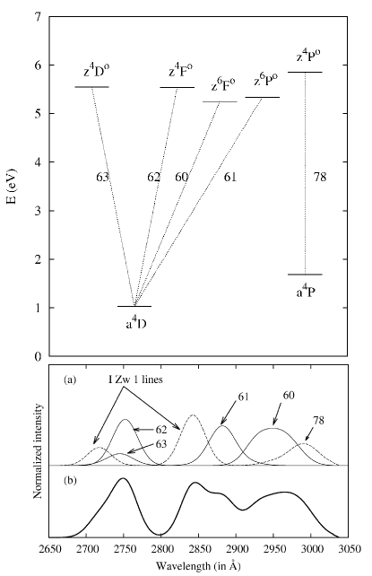
Figure 11: The Grotrian diagram of multiplets included in the UV Fe ii model (Kovačević-Dojčinović & Popović, 2015), with additional multiplet 78 (top). The example of the multiplet emission calculated for T = 10000 K, Doppler width w = 1200 km s^-1 and arbitrary intensities of multiplets (a) and total improved UV Fe ii semi-empirical model (b). The emission included in an improved version of model is denoted with dashed line (a).

Finally, the improved UV Fe ii model consists of the 5 multiplets: 60 (a${\ }^{4}D$ - z${\ }^{6}F^{o}$), 61 (a${\ }^{4}D$ - z${\ }^{6}P^{o}$ ), 62 (a${\ }^{4}D$ - z${\ }^{4}F^{o}$), 63 (a${\ }^{4}D$ - z${\ }^{4}D^{o}$) and 78 (a${\ }^{4}P$ - z${\ }^{4}P^{o}$), and empirically added ’I Zw 1 lines’ represented with Gaussians at $\lambda$2720 Å and $\lambda$2840 Å, which relative intensities are fixed to the value obtained from the best fit of I Zw 1 Fe ii lines in the UV (see Table 1, last row). The multiplets used for the UV Fe ii model are shown in Grotrian diagram in Fig. 11, with additional multiplet 78. The example of multiplets emission, with empirically added ’I Zw 1 lines’ is shown in Fig. 11a, and the shape of total UV Fe ii model is shown in 11b.

We assume that the widths and shifts of all UV Fe ii lines are the same, since they probably originate from the same emission region, so the improved UV Fe ii model has 9 free parameters: width, shift, intensity of ’I Zw 1 lines’, intensities for each of 5 multiplets, and the temperature, which is used to calculate the relative intensities of the lines within each multiplet (see Eq. (1), Sec 2.2.2). The relative intensities of the lines within each multiplet were calculated for the T = 5000 K, 10000 K and 50000 K, normalized to the strongest line in the multiplet and shown in Table 1. For calculation of the relative intensities with Eq. (1), we used the updated atomic data from National Institute of Standards and Techology (NIST) Atomic Spectra Database and Kurucz atomic database (Kurucz, 1994).

The fits of I Zw 1 and Mrk 493 with improved UV Fe ii semi-empirical model are shown in Fig 12. As it can be seen, the improved UV Fe ii model can fit very well the UV Fe ii lines in NLSy1 galaxies.

Figure 12: The fit of NLSy1 galaxies I Zw 1 (top) and Mrk 493 (bottom) with the improved UV Fe ii model, denoted with dashed line.

Kovačević et al. (2010) have found that the flux ratio of the Fe ii multiplets is not constant, i.e. it can vary from object to object. In this work, we found that the ratio of the UV Fe ii multiplets slightly differs in two observed NLSy1 galaxies: I Zw 1 and Mrk 493. Therefore, the UV Fe ii model with free parameters for multiplet intensity enables fitting the objects with different strength of Fe ii multiplets, which is not possible with other UV Fe ii templates based on I Zw 1 Fe ii emission lines, or theoretically calculated, with fixed relative intensities of UV Fe ii lines. This is an advantage of the UV Fe ii semi-empirical model that we have developed.

We compared this improved UV Fe ii model with theoretical models given in Sigut & Pradhan (2003) and Bruhweiler & Verner (2008) and empirical UV Fe ii templates based on the spectrum of I Zw 1, and presented in Tsuzuki et al. (2006) and Vestergaard & Wilkes (2001). The applied version of theoretical model from Sigut & Pradhan (2003) was calculated for photoionization model A of the BLR, with included Ly$\alpha$ and Ly$\beta$ pumping, and the applied version of theoretical model from Bruhweiler & Verner (2008) was calculated for log[$\mathrm{n_{H}}$/(cm^-3)]=11, [$\xi$]/(1 km s^-1)=20 and log[$\mathrm{\Phi_{H}}$/(cm^-2 s^-1)]=20.5.

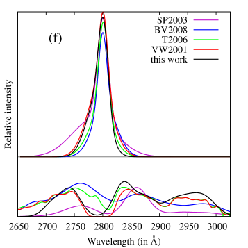
Figure 14: The same as in Fig. 13 but for object SDSS J105540.81$+$421241.2, for which we obtained the Mg ii profile with blue asymmetry with our decomposition model.

To test the different UV Fe ii templates, we chose three examples of spectra where we obtained different shapes of Mg ii lines after applying our improved UV Fe ii model: with red asymmetry in Mg ii profile (Fig. 13), with blue asymmetry in Mg ii profile (Fig. 14), and with no significant asymmetry of Mg ii (Fig. 15). We fitted these examples with different templates, and compared the obtained profiles of Fe ii and Mg ii lines with different Fe ii models (see Figs 13, 14 and 15).

It can be seen that all considered UV Fe ii templates have different shapes, which result with different spectral decomposition of Mg ii$+$UV Fe ii lines in all examples, and consequently with different shape of extracted pure Mg ii profile. The empirical templates of Tsuzuki et al. (2006) and Vestergaard & Wilkes (2001) are both made using the spectrum of the I Zw 1 galaxy, and therefore these templates are the most similar among the others, and they give the most similar fits of Mg ii$+$UV Fe ii lines. The improved UV Fe ii model presented in this work slightly vary from case to case comparing to the empirical templates, while the theoretical models of Sigut & Pradhan (2003) and Bruhweiler & Verner (2008) in some cases have larger incompatibility with other three templates.

Namely, the theoretical models of Sigut & Pradhan (2003) and Bruhweiler & Verner (2008) cannot fit well the UV Fe ii bump at $\sim$2900-3000 Å range in all given examples (see Fig. 13, 14 and 15, case (b) and (c)). The discrepancy is the strongest in the spectrum shown in Fig. 14, with strong UV Fe ii lines at $\sim$2900-3000 Å range.

The empirical templates of Tsuzuki et al. (2006) and Vestergaard & Wilkes (2001) fit well all given examples. However, in the case of complex Mg ii$+$UV Fe ii shapes (see Fig 15), the fits with these templates have small discrepancy (at $\sim$2700-2780 Å range in Fig. 15 (d), and at $\sim$2820-2840 Å range in Fig. 15 (e)). Additionally, the empirical template of Vestergaard & Wilkes (2001) has artificial cut from 2770 Å to 2819 Å (under the Mg ii emission), i.e. the UV Fe ii emission is set to zero in the range 2770–2819 Å, that also can artificially change the Mg ii broad line profiles. Therefore, we developed the semi-empirical UV Fe ii model (an improved template of Kovačević-Dojčinović & Popović, 2015) which can fit well all these different Mg ii line profiles (see Fig. 13, 14 and 15, case (a)) and is able to account possible difference between the multiplet intensities which may be caused by slight different physical conditions in the UV Fe ii emitting region. The template is available on-line, through the Serbian Virtual Observatory.

Table 1: The improved UV Fe ii $\lambda\lambda$ 2650-3050 Å model: the relative intensities of the UV Fe ii emission lines within multiplets calculated for different temperatures (see Eq. (1)) and using updated atomic data. The lines with the strength of four order of magnitude lower than the strongest line from multiplet are excluded from model, since their contribution in flux is negligible.

Wavelength	Transitions	Relative intensity
		T=5000 K	T=10000 K	T=50000 K
	multiplet  a${\ }^{4}D$ - z${\ }^{6}F^{o}$ (60)
2907.853	a${\ }^{4}D_{7/2}$ - z${\ }^{6}F^{o}_{5/2}$	0.008	0.009	0.009
2916.148	a${\ }^{4}D_{7/2}$ - z${\ }^{6}F^{o}_{7/2}$	0.006	0.006	0.006
2926.585	a${\ }^{4}D_{7/2}$ - z${\ }^{6}F^{o}_{9/2}$	1.000	1.000	1.000
2939.507	a${\ }^{4}D_{5/2}$ - z${\ }^{6}F^{o}_{3/2}$	0.015	0.016	0.016
2945.264	a${\ }^{4}D_{5/2}$ - z${\ }^{6}F^{o}_{5/2}$	0.005	0.005	0.005
2953.774	a${\ }^{4}D_{5/2}$ - z${\ }^{6}F^{o}_{7/2}$	0.835	0.849	0.861
2961.273	a${\ }^{4}D_{3/2}$ - z${\ }^{6}F^{o}_{1/2}$	0.013	0.014	0.014
2964.659	a${\ }^{4}D_{3/2}$ - z${\ }^{6}F^{o}_{3/2}$	0.012	0.013	0.013
2970.514	a${\ }^{4}D_{3/2}$ - z${\ }^{6}F^{o}_{5/2}$	0.355	0.366	0.376
2975.933	a${\ }^{4}D_{1/2}$ - z${\ }^{6}F^{o}_{1/2}$	0.025	0.027	0.028
2979.353	a${\ }^{4}D_{1/2}$ - z${\ }^{6}F^{o}_{3/2}$	0.184	0.191	0.197
	multiplet  a${\ }^{4}D$ - z${\ }^{6}P^{o}$ (61)
2833.369	a${\ }^{4}D_{7/2}$ - z${\ }^{6}P^{o}_{5/2}$	0.010	0.010	0.011
2837.737	a${\ }^{4}D_{5/2}$ - z${\ }^{6}P^{o}_{3/2}$	0.001	0.001	0.001
2861.168	a${\ }^{4}D_{3/2}$ - z${\ }^{6}P^{o}_{3/2}$	0.028	0.032	0.035
2868.875	a${\ }^{4}D_{5/2}$ - z${\ }^{6}P^{o}_{5/2}$	0.208	0.225	0.240
2874.854	a${\ }^{4}D_{1/2}$ - z${\ }^{6}P^{o}_{3/2}$	0.028	0.032	0.036
2880.7563	a${\ }^{4}D_{7/2}$ - z${\ }^{6}P^{o}_{7/2}$	1.000	1.000	1.000
2892.832	a${\ }^{4}D_{3/2}$ - z${\ }^{6}P^{o}_{5/2}$	0.077	0.083	0.088
2917.462	a${\ }^{4}D_{5/2}$ - z${\ }^{6}P^{o}_{7/2}$	0.079	0.079	0.079
	multiplet  a${\ }^{4}D$ - z${\ }^{4}F^{o}$ (62)
2692.834	a${\ }^{4}D_{7/2}$ - z${\ }^{4}F^{o}_{5/2}$	0.002	0.003	0.003
2724.884	a${\ }^{4}D_{5/2}$ - z${\ }^{4}F^{o}_{5/2}$	0.017	0.019	0.021
2730.734	a${\ }^{4}D_{3/2}$ - z${\ }^{4}F^{o}_{3/2}$	0.031	0.036	0.041
2743.197	a${\ }^{4}D_{1/2}$ - z${\ }^{4}F^{o}_{3/2}$	0.444	0.515	0.579
2746.483	a${\ }^{4}D_{3/2}$ - z${\ }^{4}F^{o}_{5/2}$	0.544	0.613	0.673
2749.321	a${\ }^{4}D_{5/2}$ - z${\ }^{4}F^{o}_{7/2}$	0.745	0.801	0.848
2755.736	a${\ }^{4}D_{7/2}$ - z${\ }^{4}F^{o}_{9/2}$	1.000	1.000	1.000
	multiplet  a${\ }^{4}D$ - z${\ }^{4}D^{o}$ (63)
2714.413	a${\ }^{4}D_{7/2}$ - z${\ }^{4}D^{o}_{5/2}$	0.132	0.139	0.144
2727.539	a${\ }^{4}D_{5/2}$ - z${\ }^{4}D^{o}_{3/2}$	0.120	0.131	0.140
2736.966	a${\ }^{4}D_{1/2}$ - z${\ }^{4}D^{o}_{3/2}$	0.056	0.063	0.068
2739.547	a${\ }^{4}D_{7/2}$ - z${\ }^{4}D^{o}_{7/2}$	1.000	1.000	1.000
2746.982	a${\ }^{4}D_{5/2}$ - z${\ }^{4}D^{o}_{5/2}$	0.519	0.544	0.565
2749.181	a${\ }^{4}D_{3/2}$ - z${\ }^{4}D^{o}_{3/2}$	0.231	0.251	0.268
2749.486	a${\ }^{4}D_{1/2}$ - z${\ }^{4}D^{o}_{1/2}$	0.106	0.118	0.128
2761.813	a${\ }^{4}D_{1/2}$ - z${\ }^{4}D^{o}_{3/2}$	0.053	0.058	0.062
2768.934	a${\ }^{4}D_{3/2}$ - z${\ }^{4}D^{o}_{5/2}$	0.022	0.023	0.024
2772.723	a${\ }^{4}D_{5/2}$ - z${\ }^{4}D^{o}_{7/2}$	0.001	0.001	0.001
	multiplet  a${\ }^{4}P$ - z${\ }^{4}P^{o}$ (78)
2944.395	a${\ }^{4}P_{3/2}$ - z${\ }^{4}P^{o}_{1/2}$	0.117	0.128	0.138
2947.655	a${\ }^{4}P_{5/2}$ - z${\ }^{4}P^{o}_{3/2}$	0.189	0.200	0.210
2964.624	a${\ }^{4}P_{1/2}$ - z${\ }^{4}P^{o}_{1/2}$	0.045	0.049	0.053
2965.032	a${\ }^{4}P_{3/2}$ - z${\ }^{4}P^{o}_{3/2}$	0.132	0.140	0.146
2984.825	a${\ }^{4}P_{5/2}$ - z${\ }^{4}P^{o}_{5/2}$	1.000	1.000	1.000
2985.545	a${\ }^{4}P_{1/2}$ - z${\ }^{4}P^{o}_{3/2}$	0.665	0.705	0.739
3002.644	a${\ }^{4}P_{3/2}$ - z${\ }^{4}P^{o}_{5/2}$	0.620	0.620	0.620
	’I Zw 1 lines’ - relative intensity of Gaussiaans
2715	0.357
2840	1

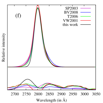
Figure 13: Fits of SDSS J135045.66$+$233145.2 with different UV Fe ii templates: (a) this work, (b) Bruhweiler & Verner (2008) (BV2008), (c) Sigut & Pradhan (2003) (SP2003), (d) Tsuzuki et al. (2006) (T2006), (e) Vestergaard & Wilkes (2001) (VW2001), and (f) comparison of the UV Fe ii lines (bottom) and Mg ii profiles (top) obtained from the best fit using different UV Fe ii models (for colored version of this Figure see electronic version). We obtained the Mg ii profile with red asymmetry after decomposition with our improved UV Fe ii model (a).

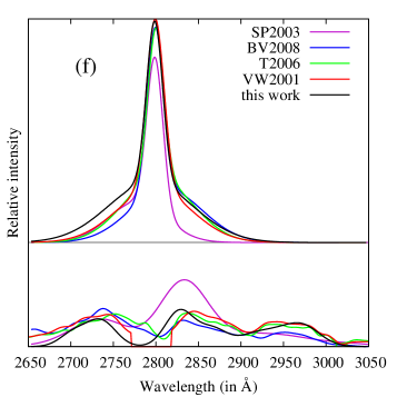
Figure 15: The same as in Fig. 13 but for object SDSS J122454.46$+$212246.4, for which we obtained nearly symmetric Mg ii profile with our decomposition model.

Appendix B Contribution of the ’fountain-like’ region and the accuracy of the BH mass measurements

We analysed the different parameters of Mg ii lines, trying to find some Mg ii line properties which indicate dominant emission from the ’fountain-like’ region and some quantitative constraints of Mg ii parameters for which Mg ii line is reliable (or not reliable) for the single epoch M_BH estimation.

Previously, in Sec. 3.1 we explored the correlation between the intrinsic shift (z_10%) and the width (FW10%M) that indicates virialization in the Mg ii emitting region. As it can be seen in Fig. 5b, the objects with the Mg ii lines with approximately z_10% $<$ -800 km s^-1, or FW10%M $>$ 12250 km s^-1, do not follow the linear correlation. In these cases, the emission of the ’fountain-like’ region is probably dominant in the wings of the Mg ii. However, we could not find the strict constraint in the Mg ii line parameters which would guarantee that the M_BH estimated using the Mg ii FWHM is reliable, or opposite, that it is much different from the M_BH estimated using H$\beta$.

Additionally we explored the correlation between the contribution of the ’fountain-like’ region to the FWHM and FWH10%M of Mg ii.

To estimate the contribution of the ’fountain-like’ region, we normalized the intensities of H$\beta$ and Mg ii to 1, then rescaled the Mg ii to have the same FWHM as H$\beta$, and measured the flux of the difference between these two line profiles [F(Mg ii)-F(H$\beta$)]. Roughly, it can be assumed that this difference is in correlation with the contribution of the ’fountain like’ region to the Mg ii line profiles. Taking 1$\sigma$ criteria, we divided our data in two subsamples: one where the disagreement between the BH masses calculated using H$\beta$ and Mg ii parameters are $<$ 1$\sigma$ (’good BH measurements’), and another where disagreement is $>$1 $\sigma$ (’bad BH measurements’). The 1 $\sigma$ = 0.19 for log[M_BH(H$\beta$)/M_BH(Mg ii)] distribution.

In Figs. 16 and 17 we present the FWHM and FW10%M of Mg ii as a function of the estimated ’fountain-like’ emission. As it can be seen in Fig. 16ab, there is no correlation between the FWHM Mg ii and the ’fountain-like’ contribution, in the both cases: in so-called ’good BH measurements’ and ’bad BH measurements’. However, there is a high correlation between FWH10%M Mg ii and ’fountain-like’ contribution in both cases (see Fig. 17ab). For subsample of ’good BH measurements’, the correlation is higher ($\rho$=0.86, $P_{0}<$10^-20), compared the one for ’bad BH measurements’ ($\rho$=0.73, $P_{0}$=10^-17). In the case of ’good BH measurements’, the correlation is higher probably because the ’fountain-like’ region contributes more to the far line wings (FWH10%M), and do not affect the FWHM that is used for BH estimates. In the case of the ’bad BH measurements’ the correlation is smaller and scattering of the points is higher, which may indicates that the ’fountain-like’ contribution is likely to be more important in the line center, and therefore the mass (and FWHM) measurements may be partly affected by contribution of this region.

Figure 16: The relationship between the FWHM Mg ii and [F(Mg ii)-F(H$\beta$)]/F(Mg ii), where F(Mg ii) and F(H$\beta$) are fluxes of Mg ii and H$\beta$ normalized to 1, and fitted to have the same FWHM. Panel (a): for subsample with log[M_BH(H$\beta$)/M_BH(Mg ii)] smaller than 1 $\sigma$ ($\sigma$ = 0.19), and Panel (b): larger than 1 $\sigma$.

Figure 17: The same as in previous figure but for FW10%M Mg ii and the [F(Mg ii)-F(H$\beta$)]/F(Mg ii).

References

- Barth et al. (2015) Barth, A.J., Bennert V. N., Canalizo, G. et al. 2015, ApJS, 217, 26
- Bentz et al. (2013) Bentz, M. C., Denney, K. D., Grier, C. J. et al. 2013, ApJ, 767, 149
- Bergeron & Kunth (1980) Bergeron, J. and Kunth, D. 1980, A&A, 85, L11
- Bon et al. (2006) Bon, E., Popović, L. Č., Ilić, D. & Mediavilla, E. G. 2006, NARev, 50, 716
- Boroson & Green (1992) Boroson, T. A., Green, R. F. 1992, ApJS, 80, 109
- Bruhweiler & Verner (2008) Bruhweiler, F., Verner, E. 2008, ApJ, 675, 83
- Coatman et al. (2017) Coatman, L., Hewett, P. C., Banerji, M., Richards, G. T., Hennawi, J. F., Prochaska, J. X. 2017, MNRAS, 465, 2120
- Collier et al. (1998) Collier, S. J., Horne, K., Kaspi, S. et al. 1998, ApJ, 500, 162
- Connolly et al. (1995) Connolly, A. J., Szalay, A. S., Bershady, M. A., Kinney, A. L., & Calzetti, D. 1995, AJ, 110, 1071
- Czerny et al. (2017) Czerny, B., Li, Y.-R., Sredzinska, J., Hryniewicz, K., Panda, S., Wildy, C., Karas, V. 2017, Frontiers in Astronomy and Space Sciences, 4, 5
- Denney (2012) Denney, K. D. 2012, ApJ, 759, 44
- Dong et al. (2008) Dong, X., Wang, T., Wang, J., Yuan, W., Zhou, H., Dai, H., Zhang, K. 2008, MNRAS, 383, 581
- Gaskell (2009) Gaskell, C. M. 2009, NewAR, 53, 140
- Hu et al. (2008) Hu, C., Wang, J.-M., Chen, Y.-M., Bian, W. H., Xue, S. J. 2008, ApJ, 683, 115
- Jonić et al. (2016) Jonić, S., Kovačević-Dojčinović, J., Ilić, D., and Popović, L. Č. 2016, Ap&SS, 361, 101.
- Kollatschny & Zetzl (2013) Kollatschny, W., Zetzl, M. 2013, A&A, 558A, 26
- Kovačević-Dojčinović & Popović (2015) Kovačević-Dojčinović, J., Popović, L. Č. 2015, ApJS, 189, 15
- Kovačević et al. (2010) Kovačević, J., Popović, L. Č., Dimitrijević, M.S. 2010, ApJS, 189, 15
- Kovačević et al. (2014) Kovačević, J., Popović, L. Č., Kollatschny, W. 2014, ASR, 54, 1347
- Kuraica et al. (2009) Kuraica, M. M., Obradović, B. M., Cvetanović, N., Dojčinović, I. P., Purić, J. 2009, NewAR, 52, 266
- Kurucz (1994) Kurucz, R. 1994, Kurucz CD-ROM No. 22 (Smithsonian Astrophysical Observatory, Cambridge, 1994)
- Laor et al. (1997) Laor, A., Jannuzi, B. T., Green, R. F., Boroson, T. A. 1997, ApJ, 489, 656
- Lakićević et al. (2017) Lakićević, M., Kovačević-Dojčinović, J., Popović, L. Č. 2017, MNRAS, 472, 334
- León-Tavares et al. (2013) León-Tavares, J., Chavushyan, V., Patiño–Alvarez, V. et al. 2013, ApJ, 763L, 36
- Liu et al. (2017) Liu, H. T., Feng, H. C., Bai, J. M. 2017, MNRAS, 466, 3323
- Marziani & Sulentic (2012) Marziani, P., Sulentic, J. W. 2012, NewAR, 56, 49
- Marziani et al. (2013a) Marziani, P., Sulentic, J. W., Plauchu-Frayn, I., del Olmo, A. 2013a, A &A, 555, 89
- Marziani et al. (2013b) Marziani, P., Sulentic, J. W., Plauchu-Frayn, I., del Olmo, A. 2013b, ApJ, 764, 150
- McLure & Dunlop (2004) McLure, R. J., Dunlop, J. S. 2004, MNRAS, 352, 1390
- Mejía-Restrepo et al. (2018) Mejía-Restrepo, J. E., Lira, P., Netzer, H., Trakhtenbrot, B., Capellupo, D. M. 2018, NatAs, 2, 63
- Mejía-Restrepo et al. (2016) Mejía-Restrepo, J. E., Trakhtenbrot, B., Lira, P., Netzer, H., Capellupo, D. M. 2016, MNRAS, 460, 187
- Netzer (2015) Netzer, H. 2015,ARA&A, 53, 365
- Onken & Kollmeier (2008) Onken, C. A. & Kollmeier, J. A. 2008, ApJ, 689L, 13
- Peebles (1993) Peebles P.J.E. 1993, Principles of Physical Cosmology, Princeton University Press, Princeton
- Peterson (1993) Peterson, B. M. 1993, PASP, 105, 207
- Peterson (2014) Peterson, B. M. 2014, SSRv, 183, 253
- Popović & Kovačević (2011) Popović, L. Č. & Kovačević, J. 2011, ApJ, 738, 68
- Popović et al. (2004) Popović, L. Č., Mediavilla, E., Bon, E., & Ilić, D. 2004 A&A 423, 909
- Popović et al. (2002) Popović, L. Č., Mediavilla, E. G., Kubičela, A., Jovanović, P. 2002, A&A, 390, 473.
- Shapovalova et al. (2012) Shapovalova, A. I., Popović, L. Č., Burenkov, A. N. et al. 2012, ApJS, 202, 10
- Shen & Liu (2012) Shen, Y., Liu, X. 2012, ApJ, 753, 125
- Sigut & Pradhan (2003) Sigut, T. A. A.& Pradhan, A. K. 2003, ApJS, 145, 15
- Sulentic et al. (2000a) Sulentic, J. W., Marziani, P., Dultzin-Hacyan, D. 2000a, ARA&A, 38, 521
- Sulentic et al. (2014) Sulentic, J. W., Marziani, P., Olmo, A., Plauchu-Frayn, I., 2014, ASR, 54, 1406
- Sulentic et al. (2000b) Sulentic, J. W., Zwitter, T., Marziani, P., Dultzin-Hacyan, D. 2000b, ApJ, 536, 5
- Tilton & Shull (2013) Tilton, E. M., Shull, J. M. 2013, ApJ, 774, 67
- Trakhtenbrot & Netzer (2012) Trakhtenbrot, B., Netzer, H. 2012, MNRAS, 427, 3081
- Tsuzuki et al. (2006) Tsuzuki, Y., Kawara, K., Yoshii, Y., Oyabu, S. 2006, 650, 57
- Vanden Berk et al. (2006) Vanden Berk, D. E., Shen, J., Yip, C.-W. et al. 2006, AJ, 131, 84
- Veŕon-Cetty et al. (2004) Veŕon-Cetty, M.-P., Joly, M., Veŕon, P. 2004, A&A, 384, 826
- Vestergaard & Osmer (2009) Vestergaard, M., Osmer, P. S. 2009, ApJ, 699, 800
- Vestergaard & Peterson (2006) Vestergaard, M., Peterson, B. M. 2006, ApJ, 641, 689
- Vestergaard & Wilkes (2001) Vestergaard, M., Wilkes, B. J. 2001, ApJS, 134, 1
- Wang et al. (2009) Wang, J.-G., Dong, X.-B., Wang, T.-G., Ho, L. C., Yuan, W., Wang, H., Zhang, K., Zhang, S., Zhou, H. 2009, ApJ, 707, 1334
- Yip et al. (2004a) Yip, C. W., Connolly, A. J., Szalay, A. S. et al. 2004a, AJ, 128, 585
- Yip et al. (2004b) Yip, C. W., Connolly, A. J., Vanden Berk, D. E. et al. 2004b, AJ, 128, 2603