Variation Network: Learning High-level Attributes for Controlled Input Manipulation

Abstract

This paper presents the Variation Network (VarNet), a generative model providing means to manipulate the high-level attributes of a given input. The originality of our approach is that VarNet is not only capable of handling pre-defined attributes but can also learn the relevant attributes of the dataset by itself. These two settings can also be easily considered at the same time, which makes this model applicable to a wide variety of tasks. Further, VarNet has a sound information-theoretic interpretation which grants us with interpretable means to control how these high-level attributes are learned. We demonstrate experimentally that this model is capable of performing interesting input manipulation and that the learned attributes are relevant and meaningful.

1 Introduction

We focus on the problem of learning to generate variations of a given input in an intended way. Concretely, this means that given some input element $x$, which can be considered as a template, we want to generate some transformed versions of $x$ by only modifying its high-level attributes. The objective is that the link between the original $x$ and its transformed version is preserved while the difference between their attributes is patent. Such a mechanism can be of great use in many domains such as image edition since it allows to edit images using more abstract controls and can be of crucial importance for creative usages since it allows to generate new content in a controlled and meaningful way.

In a majority of the recent proposed methods tackling this problem such as [29, 18, 27], the attributes of interest that we want to control are assumed to be given (often given as a discrete variable). If these methods are indeed successful in generating meaningful transformations of any input, we can nonetheless identify two shortcomings which can restrict their use: 1) Labeled data is not always available or can be costly to obtain; 2) Attributes which can be hard to specify in an absolute way cannot be considered.

The novelty of our approach resides in the fact that it grants the possibility, under the same framework, to control generations by modifying user-specified attributes but also to learn some meaningful high-level attributes at the same time, which can be used for control.

This problem may seem to be an ill-posed one on many aspects: Firstly, in the case of specified attributes, there is no ground truth for variations since there is no $x$ with two different attributes. Secondly, it can be hard to determine if a learned attribute is relevant. However, we provide empirical evidence that our general approach is capable of learning such relevant attributes and that they can be used for generating meaningful variations.

This paper introduces the Variation Network (VarNet), a probabilistic neural network which provides means to manipulate an input by changing its high-level attributes, which can be either learned or provided. Our model has a sound probabilistic interpretation which makes the variations obtained by changing the attributes statistically meaningful. This architecture is general and provides a wide range of design choices.

Our contributions are the following:

• A widely applicable encoder-decoder architecture which generalizes existing approaches [16, 26, 18, 27] on controlled input manipulation,

• An easy-to-use framework: any encoder-decoder architecture can be easily framed into our framework in order to provide it control over generations, even in the case of unlabeled data,

• Information-theoretic interpretation of our model providing a way to control the behavior of the learned attributes.

The plan of this paper is the following: Sect. 2 presents the VarNet architecture together with its training algorithm. For better clarity, we introduce separately all the components featured in our model and postpone the discussion about their interplay and the motivation behind our modeling choices in Sect. 3 We illustrate in Sect. 4 the possibilities offered by our proposed model and show that its faculty to generate variations in an intended way is of particular interest. Finally, Sect. 5 discusses about the related works. In particular, we show that VarNet provides an interesting solution to many constrained generation problems already considered in the literature while bearing interesting connections with the literature in fair representations [22, 27] and disentangled representations [12, 2, 21].

Our code is available at https://github.com/Ghadjeres/VarNet.

2 Proposed model

We now introduce our novel encoder-decoder architecture which we name Variation Network. Our architecture borrows principles from the traditional Variational AutoEncoder (VAE) architecture [16] and from the Wasserstein AutoEncoder (WAE) architecture [28, 26]. It uses an adversarially learned regularization [7, 18], introduces a decomposition of the latent space into two parts, a template $z$ and an attribute $\psi$ [1] and decomposes the attributes on an adaptive basis [30].

We detail in the following sections the different parts involved in our model. In Sect. 2.1, we focus on the encoder-decoder part of VarNet, in Sect. 2.2, we introduce the adversarially-learned regularization whose aim is to disentangle attributes from templates and in Section 2.3, we discuss about the special parametrization that we adopted for the space of attributes.

2.1 Encoder-decoder part

We consider a dataset $\mathcal{D}=\{(x^{(1)},m^{(1)}),\dots,(x^{(N)},m^{(N)})\}$ of $N$ labeled elements $(x,m)\in\mathcal{X}\times\mathcal{M}$, where $\mathcal{X}$ stands for the input space and $\mathcal{M}$ for the metadata space. Here, metadata information is optional as our architecture is also applicable in the totally unsupervised case. We suppose that the $x$’s follow the data distribution $\pi(x)$, that for each $x\in\mathcal{X}$ corresponds a unique label $m$ and write $\pi(x,m)$ the distribution of the $x$’s together with their metadata information.

Similar to the VAE architectures, we suppose that our data $x\in\mathcal{X}$ depends on a couple of low-dimensional latent variable $z\in\mathcal{Z}\subset\mathbf{R}^{d_{z}}$ and $\psi\in\Psi\subset\mathbf{R}^{d_{\psi}}$ through some decoder $p(x|z,\psi)$ parametrized by a neural network. In this paper, we term the $z$ variables templates and the $\psi$ variable attributes. More details about the attribute space $\Psi$ are given in Sect. 2.3.

We introduce a factorized prior $p(z,\psi)=p(z)p(\psi)$ over this latent space so that the joint probability distribution is expressed as $p(x,z,\psi)=p(x|z,\psi)p(z)p(\psi)$. The objective is to maximize the log-likelihood $\mathbf{E}_{(x,m)\sim\mathcal{D}}\log\pi(x)$ of the data under the model. Since the posterior distribution $p(z|x)$ is usually intractable, an approximate posterior distribution $q(z|x)$ parametrized by a neural network is introduced (for simplicity, we let the approximate posterior depend on $x$ only, but considering $q(z|x,m)$ or even $q(z|x,\psi)$ is feasible). Concerning the computation of $\psi$ given $x$, we introduce a deterministic function $f(x,m)$ parametrized by a neural network, which can eventually rely on metadata information $m$.

We then obtain the following mean reconstruction loss:

$$\mathrm{RE}:=-\mathbf{E}_{(x,m)\sim\pi}\mathbf{E}_{z\sim q(z|x)}\log p(x|z,f(x,m)),$$ (1)

and regularize the latent space $\mathcal{Z}$ by adding the usual Kullback-Leibler ($\mathrm{KL}$) divergence term appearing in the VAE Evidence Lower Bound (ELBO) on $\mathcal{Z}$:

$$\mathrm{KL}:=\mathbf{E}_{z\sim q(z|x)}\log\frac{q(z|x)}{p(z)}.$$ (2)

2.2 Disentangling attributes from templates

Our decoder $p(x|z,\psi)$ thus depends exclusively on $z$ and on features $\psi$. However, there is no reason for a random attribute $\psi\in\Psi\neq f(x,m)$ that $\hat{x}\sim p(.|z,\psi)$, where $z\sim q(z|x)$, is a meaningful variation of the original $x$. Indeed, all needed information for reconstructing $x$ could potentially be already contained in $z$ and changing $\psi$ could have no effect on the reconstructions.

To enforce this property, we propose to add an adversarially-learned cost on the latent variables $z$ and $\psi$ to force the encoder $q$ to discard information about the attribute $\psi=f(x,m)$ of $x$: Specifically, we train a discriminator neural network $D:\mathcal{Z}\times\Psi\to[0,1]$ whose role is to evaluate the probability $D(z,\psi)$ that there exists a pair $(x,m)\in\mathcal{D}$ such that $\psi=f(x,m)$ and $z\sim q(z|x)$. In other words, the aim of the discriminator is to determine if the attributes $\psi$ and the template code $z$ originate from the same $(x,m)\in\mathcal{D}$ or if the features $\psi$ are sampled from the prior $p(\psi)$.

The encoder-decoder architecture presented in Sect. 2.1 is trained to fool the discriminator: this means that, for a given $(x,m)\in\mathcal{D}$, it tries to produce a template code $z\sim q(z|x)$ and features $\psi=f(x,m)$ such that no information about the features could be recovered from $z$.

In an optimal setting, i.e. when the discriminator is unable to match any $z\in\mathcal{Z}$ with a particular feature $\psi\in\Psi$, the space of template codes and the space of attributes are decorrelated and the aggregated distribution of the $\psi$’s $f_{*}(\pi)$ (the pushforward measure of $\pi$ by $f$) matches the prior $p(\psi)$.

The discriminator is trained to maximize

$$\mathcal{L}_{\mathrm{Disc}}:=\mathbf{E}_{(x,m)\sim\pi}\mathbf{E}_{z\sim q(z|x)}\mathbf{E}_{\psi\sim p(\psi)}\big{[}\log D(z,\psi)+\log(1-D(z,f(x,m)))\big{]}.$$ (3)

while the encoder-decoder architecture is trained to minimize

$$\mathcal{R}_{\mathrm{Disc}}:=-\mathbf{E}_{(x,m)\sim\pi}\mathbf{E}_{z\sim q(z|x)}\mathbf{E}_{\psi\sim p(\psi)}\big{[}\log D(z,f(x,m))+\log(1-D(z,\psi))\big{]}.$$ (4)

This is the same setting as in [7, 28] but other GAN training methods could be considered [34]. Note the presence of two terms in Eq. (4), since the “true” examples depend on training parameters.

The final objective we minimize for the encoder-decoder architecture is a combination of a reconstruction loss Eq. (1), a Kullback-Leibler penalty on $z$ Eq. (2) and the adversarially-learned loss Eq. (4).

Our final architecture is shown in Fig. 1 and the proposed training procedure in shown in Alg.1. Estimators of Eq. (3), Eq. (1) and (4) are given by Eq. (5), Eq. (7) and (8) respectively. The the estimator $\mathrm{KL}_{n}$ of the KL term can be either sampled or computed in closed form.

Figure 1: VarNet architecture. The input $x$, and its reconstruction $\hat{x}$ are in the input space $\mathcal{X}$, the metadata $m$ is in the metadata space $\mathcal{M}$, the latent variable $z$ lies in $\mathcal{Z}$ the latent template space and the attributes $\psi$ are in the attribute space $\Psi$. Dotted arrows represent identity mappings, filled arrows represent neural networks and the circled plus sign represents the concatenation of its two incoming arguments. The discriminator $D$ acts on $\mathcal{Z}\times\Psi$.

Algorithm 1 Variation Network training procedure

0:  Dataset $\mathcal{D}=\left\{(x^{(i)},m^{(i)}\right\}_{i=1..N}$, reconstruction cost $c$,reproducing kernel $k$, batch size $n$

1:  for Fixed number of iterations do

2:     Sample $x:=(x_{1},\dots,x_{n})$ and $m:=(m_{1},\dots,m_{n})$ where $(x_{i},m_{i})$ are i.i.d. samples from $\mathcal{D}$

3:     Sample $z_{i}\sim q(z|x_{i})$

4:     Sample $\hat{x}:=\{\hat{x}_{1},\dots,\hat{x}_{n}\}$ where $\hat{x}_{i}\sim p(x|z_{i},f(x_{i},m_{i})$,

5:     Sample random features $\{\psi_{i}\}_{i=1..n}\sim p(\psi)$

6:     Discriminator training phase

7:     Compute

$$\mathcal{L}_{\textrm{Disc},n}:=\frac{1}{n}\sum_{i=1}^{n}\log D\left(z_{i},\psi_{i}\right)+\log\left(1-D(z_{i},f(x_{i},m_{i}))\right)$$ (5)

8:     Gradient ascent step on the discriminator parameters using $\nabla\mathcal{L_{\textrm{Disc}}}$

9:     Encoder-decoder training phase

10:     Compute

$$\mathcal{L}_{\mathrm{EncDec},n}:=\mathrm{RE}_{n}+\beta\mathrm{KL}_{n}+\gamma\mathcal{R}_{\mathrm{Disc},n}$$ (6)

where

$$\mathrm{RE}_{n}:=-\frac{1}{n}\sum_{i=1}^{n}\log p(x_{i}|z_{i},f(x_{i},m_{i})),$$ (7)

$$\mathcal{R}_{\mathrm{Disc},n}=-\frac{1}{n}\sum_{i=1}^{n}\log D(z_{i},f(x_{i},m_{i}))+\log(1-D(z_{i},\psi_{i})).$$ (8)

11:     Gradient ascent step on all parameters except on the discriminator parameters using $\nabla\mathcal{L_{\textrm{EncDec}}}$

12:  end for

2.3 Parametrization of the attribute space

We adopt a particular parametrization of our attribute function $f:\mathcal{X}\times\mathcal{M}$. In the following, we make a distinction between two different cases: the case of continuous free attributes and the case of fixed continuous or discrete attributes.

2.3.1 Free attributes

In order to handle free attributes, which denote attributes that are not specified a priori but learned we introduce $d$ attribute vectors $v_{i}$ of dimension $d_{\psi}$ together with an attention module $\alpha:\mathcal{X}\times\mathcal{M}\to[0,1]^{d}$. By denoting $\alpha_{i}$ the coordinates of $\alpha$, we then write our attribute function $f$ as

$$f(x,m)=\sum_{i=1}^{d}\alpha_{i}(x,m)v_{i}.$$ (9)

This approach is similar to the style tokens approach presented in [30]. The $v_{i}$’s are global and do not depend on a particular instance $(x,m)$. By varying the values of the $\alpha_{i}$’s between $[0,1]$, we can then span a $d$-dimensional hypercube in $\mathbf{R}^{d_{\psi}}$ which stands for our attribute space $\Psi$. It is worth noting that the $v_{i}$’s are also learned and thus constitute an adaptive basis of the attribute space.

The prior $p(\psi)$ over $\Psi$ (note that this subspace also varies during training) is obtained by pushing forward fixed distribution $\nu_{\alpha}$ over $[0,1]^{d}$ (often considered to be the uniform distribution) using Eq. (10):

$$\psi\sim p(\psi)\quad\Longleftrightarrow\quad\psi=\sum_{i=1}^{d}\alpha_{i}v_{i}\quad\textrm{where}\quad\alpha_{i}\sim\nu_{\alpha}.$$ (10)

2.3.2 Fixed attributes

We now suppose that the metadata variable $m\in\mathcal{M}$ contains attributes that we want to vary at generation time. For simplicity, we can suppose that this metadata information can be either continuous with values in $[0,1]^{M}$ (with a natural order on each dimension) or discrete with values in $[|0,M|]$.

In the continuous case, we write our attribute function

$$f(x,m)=\sum_{i=1}^{M}m_{i}v_{i}$$ (11)

while in the discrete case, we just consider

$$f(x,m)=e_{m},$$ (12)

where $e_{m}$ is a $d_{\psi}$-dimensional embedding of the symbol $m$. It is important to note that even if the attributes are fixed, the $v_{i}$’s or the embeddings $e_{m}$ are learned during training.

These two equations define a prior $p(\psi)$ via:

$$\psi\sim p(\psi)\quad\Longleftrightarrow\quad\psi=f(x,m)\quad\textrm{where}\quad(x,m)\sim\mathcal{D}.$$ (13)

3 Comments

We now detail our objective (6) and notably explicit connections in Sect. 3.1 with [27] which gives an information-theoretic interpretation of a similar objective. In Sect. 3.2, we further discuss about the multiple possibilities that we have concerning the implementation of the attribute function and list, in Sect. 3.3, the different sampling schemes of VarNet.

3.1 Information-theoretic interpretation

Our objective bears similarity the objective Eq. (11) from [27] which is derived from the following optimization problem

$$\max I(x;z|\psi)\quad\textrm{with}\quad I(z;\psi)<\epsilon,$$ (14)

where $I(\cdot;\cdot)$ and $I(\cdot;\cdot|\cdot)$ denote the mutual information and the conditional mutual information respectively (using the joint distribution $q(x,z,f(x,m))=\pi(x,m)q(z|x)$).

The differences between our work and [27] are the following: First, our objective Eq. (6) is motivated from a generative point of view, while the motivation in [27] is to obtain fair representations ([22, 33, 24]). This allows us to consider attributes computed from both $x$ and $m$, while in [27] we have $\psi=f(x,m)=m$ and the “sensitive attributes” $m$ must be provided. A second difference is our formulation of the discriminator function: [27] considers training a discriminator to predict $\psi$ given $z$. In our case, such a formulation would prevent us to impose a prior distribution over $\Psi$.

The connection with the work of [27] thus provides an interpretation of hyperparameters $\beta$ and $\gamma$ in Eq. (6).

3.2 Flexibility in the choice of the attribute function

In this section, we focus on the parametrization of the attribute function $f:\mathcal{X}\times\mathcal{Z}\mapsto\mathbf{R}^{d}$. The formulation of Sect. 2.3 is in fact too restrictive and considered only particular attribute functions. It is in fact possible to mix different attribute functions by simply concatenating the resulting vectors. By doing so, we can then combine free and fixed attributes in a natural way but also consider different attention modules $\alpha$ similarly to what is done in [4], but also consider different distributions over the attention vectors $\alpha_{i}$.

It is important to note that the free attributes presented in Sect. 2.3.1 can only capture global attributes, which are attributes that are relevant for all elements of the dataset $\mathcal{D}$. In the presence of discrete labels $m$, it can be interesting to consider label-dependent free attributes, which are attributes specific to a subset of the dataset. In this case, the attribute function $f$ can be written as

$$f(x,m)=\sum_{i=1}^{d}\alpha_{i}(x,m)e_{m,i},$$ (15)

where $e_{m,i}$ designates the $i^{th}$ attribute vector of the label $m$. With all these possibilities at hand, it is possible to devise numerous applications in which the notions of template and attribute of an input $x$ may have diverse interpretations.

Our choice of using a discriminator over $\Psi$ instead of, for instance, over the values of $\alpha$ themselves allow to encompass within the same framework discrete and continuous fixed attributes. This also makes the combinations of such attribute functions natural.

3.3 Sampling schemes

We quickly review the different sampling schemes of VarNet. We believe that this wide range of usages makes VarNet a promising model for a wide range of applications. We can for instance:

• generate random samples $\hat{x}$ from the estimated dataset distribution:

  $$\hat{x}\sim p(x|z,\psi)\quad\textrm{with}\quad z\sim p(z)\quad\textrm{and}\quad\psi\sim p(\psi),$$ (16)

• sample $\hat{x}$ with given attributes $\psi$:

  $$\hat{x}\sim p(x|z,\psi)\quad\textrm{with}\quad z\sim p(z),$$ (17)

• generate variations of an input $x$ with attributes $\psi$:

  $$\hat{x}\sim p(x|z,\psi)\quad\textrm{with}\quad z\sim q(z|x),$$ (18)

• generate random variations of an input $x$:

  $$\hat{x}\sim p(x|z,\psi)\quad\textrm{with}\quad z\sim q(z|x)\quad\textrm{and}\quad\psi\sim p(\psi).$$ (19)

In the case of continuous attributes of the form Eq. (9) or (11), VarNet also provides a new way to generate interpolations, since we can perform interpolations either on $z$ or on $\psi$.

4 Experiments

We now illustrate the different sampling schemes presented in Sect. 3.3 on different image datasets. Section 4.1 is devoted to the implementation details and our particular modeling choices, Sect. 4.2 and 4.3 showcase some applications of VarNet ensuring that the learned attributes are meaningful and controllable. Finally, Sect. 4.4 discusses the impact of the modeling choices.

4.1 Implementation details

In all these experiments, we choose to use a ResNet-50 [11] for the encoder network. We also use a ResNet-50 for the attribute function $f$ when the function $f$ depends on the input $x$ and not only on metadata information $m$. For the decoder network, we use a conditional transposed ResNet-50 similar to the decoder used in [15]. The batch normalization parameters [13] are conditioned by $\psi$ similarly to what is done in [8, 25].

Following [6], we consider a simple parametrization for the encoder $q(z|x)$ and decoder $p(x|z,\psi)$ networks: the encoder $q(z|x)$ is a diagonal Gaussian distribution $\mathcal{N}(\mu_{z}(x),\textrm{diag}(\sigma_{z}(x)))$ and the decoder $p(x|z,\psi)$ is a diagonal Gaussian distribution with scalar covariance matrix $\mathcal{N}(\mu_{x}(z,\psi),\sigma_{x}I)$, where $\sigma_{x}$ is a learnable scalar parameter and where $I$ denotes the identity matrix.

The prior $p(z)$ over $\mathcal{Z}$ is a unit centered Normal distribution. For the sampling of the $\alpha$ values in the free attributes case, we considered $\nu_{\alpha}$ to be a uniform distribution over $[0,1]^{d}$. In the fixed attribute case, we simply obtain a random sample $\{\psi_{i}\}_{i=1}^{n}$ by shuffling the already computed batches of $\{f(x_{i},m_{i})\}_{i=1}^{n}$ (lines 4 and 6 in Alg.1).

The dimension of the template space $\mathcal{Z}$ is $d_{z}=16$ for applications on the MNIST [19], KMNIST [5], Fashion-MNIST [32] and dSprites [12, 23] datasets; and is equal to $d_{z}=64$ on the CelebA dataset [20] with resolution $64\times 64$. The hyperparameter $\beta$ and $\gamma$ in Eq. (6) are chosen equal to $1$ and $10$ respectively.

4.2 Influence of the attribute function

We now apply VarNet on the different image datasets mentioned above in order to illustrate the different sampling schemes presented in Sect. 4 and the influence of the choice of the attribute functions (Sect. 3.2). We primarily focus on sampling schemes Eq. (18) and Eq. (19) which help understanding the effect of the learned attributes.

4.2.1 Fixed discrete attributes

We start by considering attribute functions $f$ depending exclusively on discrete labels $m$ (Eq. (12)). Figure 2 shows the effect of changing the attributes of a given input $x$ using Eq. (18) on the MNIST and KMNIST datasets. We observe consistency between all variations. In these two cases, the template $z$ encompasses the handwriting and it is interesting noting that characters with two distinct way of writing appear in the generated variations.

(a)

(b)

Figure 2: Visualization of the spanned space of variations for an attribute function on MNIST (a) and KMNIST (b). The original input $x$ is shown on the bottom left of each image and the reconstructions for all 10 labels are shown on the upper line.

4.2.2 Free continuous attributes

We now focus on the case where we let the network learn relevant attributes of the data. Figure 3 displays typical examples of variations obtained by considering free attributes of dimension $d=2$ on different datasets. These plots are obtained by varying the $\alpha_{i}$ in Eq. (10) at a constant speed between 0 and 1.

(a)

(b)

(c)

Figure 3: Visualization of the spanned space of variations obtained by varying uniformly a 2-dimensional learned free attribute on different datasets: (a) MNIST (b) dSprites (c) CelebA. The initial input $x$ is displayed on the bottom left of each plot.

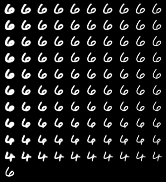
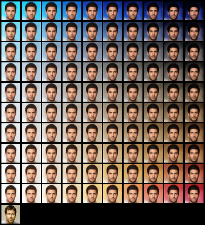
In all cases, the learned attributes are relevant to the dataset and meaningful. We find interesting to note that there is no disentanglement between the dimensions of the attributes and that the learned attributes are highly dependent on the dataset at hand.

4.2.3 Mixing attributes

In this part, we give examples of attribute functions obtained by combining the ones mentioned in the preceding sections. In particular, we consider attribute functions created by combining

• several discrete fixed attributes,

• discrete fixed attributes and continuous free attributes,

• continuous free attributes conditioned by discrete fixed attributes.

The objective is to showcase how the design of the attribute functions influences the learned attributes and the “meaning” of the templates $z$.

Figure 4: Visualization of the spanned space of variations for an attribute function depending on 2 binary labels, “Smiling” (in lines) and “Pale Skin” (in columns), on CelebA. The original input is shown on the left.

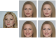
Figure 4 considers the case where two attribute functions relying solely on binary labels are concatenated. We observe that the resulting model allow to vary independently every label during generation. Such a design choice can be useful since concatenating two attributes functions taking into account two different labels instead of choosing a unique attribute function taking into account a Cartesian product of labels tends to make generalization easier.

We now consider the case where the free attributes are combined with fixed attributes. There are two different ways to do so: one is to concatenate a attribute function on free attributes with one taking into account fixed discrete attributes, the other is to make the free attributes label-dependent as in Eq. (15).

(a)

(b)

Figure 5: Visualization of the spanned space of variations: (a) for attributes being the concatenation of a fixed discrete attribute and a 1-dimensional free attribute on MNIST, (b) for a 1-dimensional label-dependent attribute Eq.15) on Fashion-MNIST.

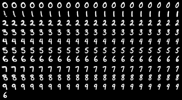
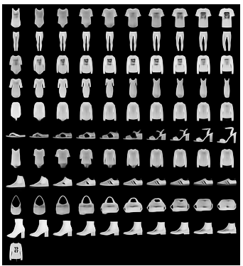
Figure 5(a) displays one such example in the first case. This corresponds to an attribute function $f$ as in Eq. (15), but where the dependence of $\alpha_{i}$ on $m$ is dropped. This results in the fact that the learned free attributes are global and possess the same “meaning” for all classes. In Fig. 5(b), on the contrary, the dependence of the $\alpha_{i}$’s on $m$ is kept. This has the effect that each class possesses a “local” free attribute.

4.3 Influence of the hyperparameters

From the preceding examples of Sect. 4.2, we saw that the fixed label attributes have clearly been taken into account, but it can be hard to guess a priori which high-level attribute the free attribute function might capture. However, for a given architecture, a given dataset and fixed hyperparameters, we observed that the network tended to learn the same high-level features across multiple runs. In this section, we show that the information-theoretic interpretation from Sect. 3.1 gives us an additional way to control what is learned by the free attributes by modifying the hyperparameter $\beta$ and/or $\gamma$.

(a)

(b)

Figure 6: Figures 6(a) and 6(b) display the space of variations using a 2-dimensional free attribute on MNIST. Figure 6(b) was generated using a model trained with a low KL penalty ($\beta=0.1$). The closest generation from the input lies in the red square.

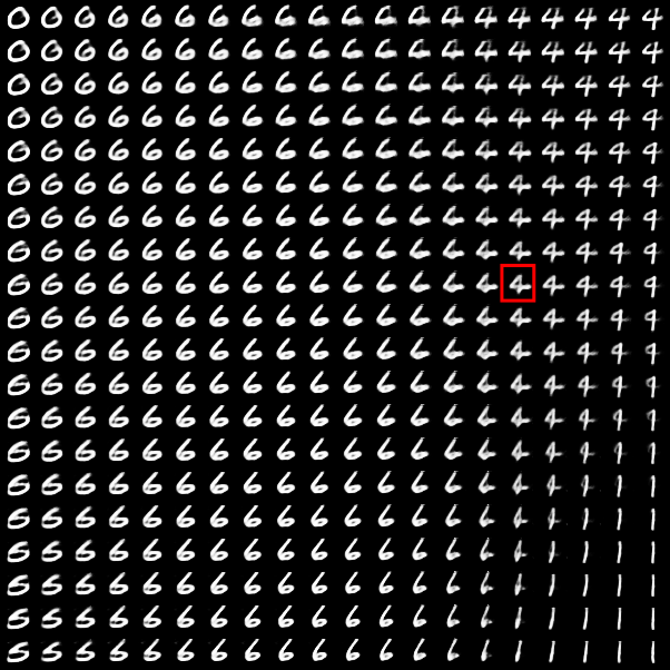
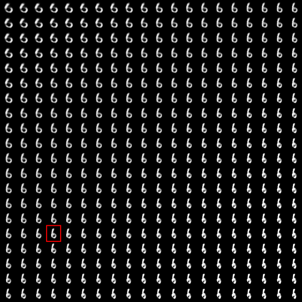
For some applications, variation spaces such as the one displayed in Fig. 6(a) are not desirable because they may tend to move too “far away” from the original input. As discussed in Sect. 3.1, it is possible to reduce how “spread” the spaces of variation are by modifying the $\beta$ parameter multiplying the KL term in the objective Eq. (6). An example of such a variation space is displayed in Fig. 6(b). If the interpretation of the high-level features learned by the free attributes seems identical in both cases, the variations spanned in 6(b) are all more similar from the original input.

4.4 Inductive biases

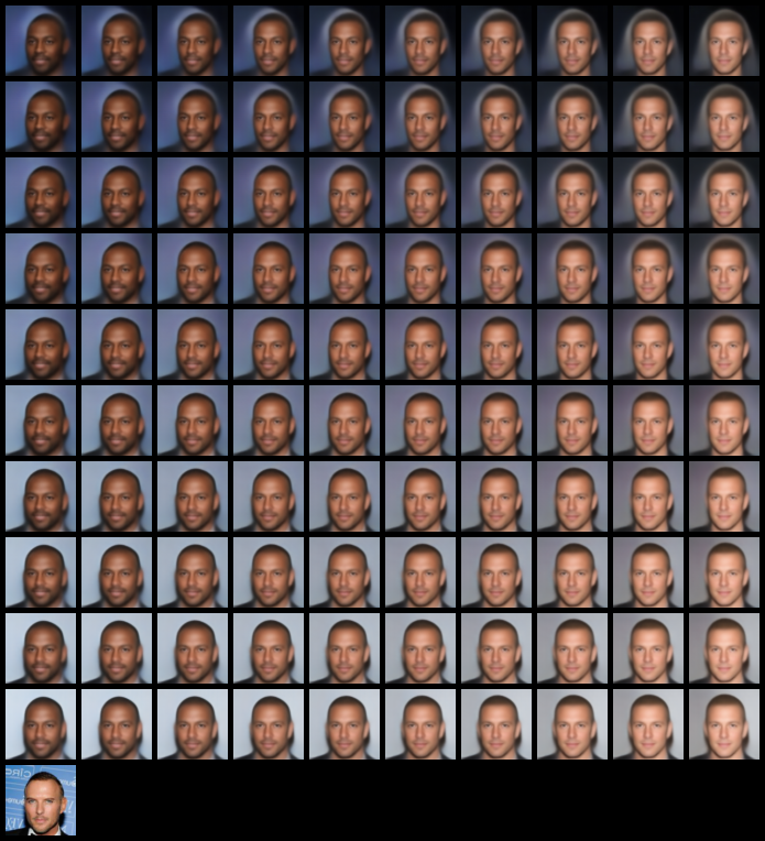
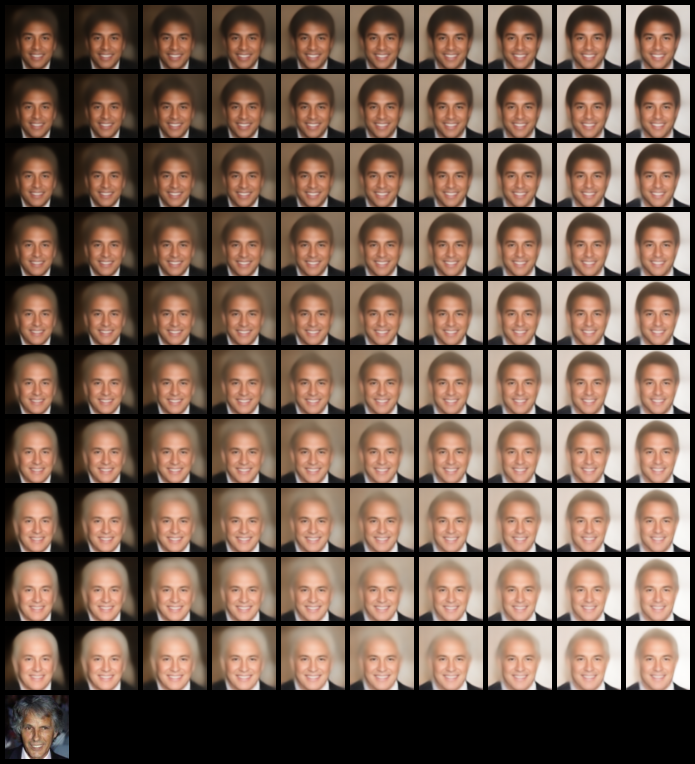
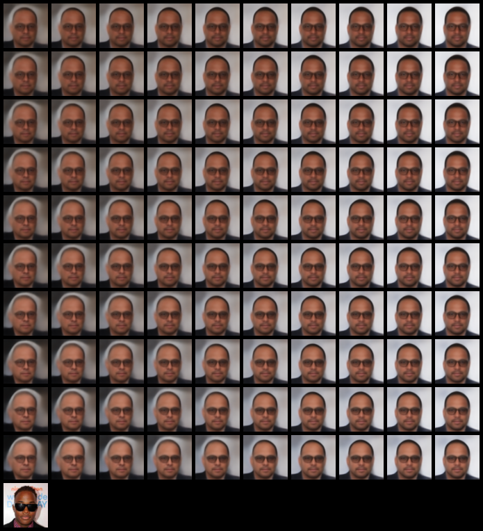
In order to check how crucial is the choice of the architecture for the encoder and the decoder, we choose in this part to train a VarNet on representations obtained from a pre-trained VAE, similarly to the TwoStageVAE from [6]. The first pre-trained VAE has the same encoder as the one described in Sect. 4.1 and a transposed VarNet-50 decoder. For the encoder and decoder of the VarNet trained on these representations, we use simple three-layered MLPs. The attribute function network is, as in Sect. 4.1, a VarNet-50. The results in the case of a 2-dimensional free attribute are displayed in Fig. 7. One striking observation is the difference with Fig. 3(c) where changing the free attributes corresponded to changing the background color. Such difference is not surprising [21] and both cases could be useful: removing information about background color in $z$ could be of help for some downstream tasks where this piece of information is irrelevant. Here, in the case of 7, the free attributes tend to learn the “pose” and “skin color” high-level attributes. This seems to be consistent across different runs (e.g. Fig. 7(a) and 7(b)) and consistent on different inputs (e.g. Fig. 7(b) and 7(c)).

(a)

(b)

(c)

Figure 7: Space of variations using a 2-dimensional free attribute on CelebA. The Variation Network is trained on representations obtained from a pre-trained VAE. Figures (b) and (c) are generated using the same model.

5 Related work

The Variation Network generalizes many existing models used for controlled input manipulation by providing a unified probabilistic framework for this task. We now review the related literature and discuss the connections with VarNet.

The problem of controlled input manipulation has been considered in the Fader networks paper [18], where the authors are able to modify in a continuous manner the attributes of an input image. Similar to us, this approach uses an encoder-decoder architecture together with an adversarial loss used to decouple templates and attributes. The major difference with VarNet is that this model has a deterministic encoder which limits the sampling possibilities as discussed in Sect. 4.3. Also, this approach can only deal with fixed attributes while VarNet is able to also learn meaningful free attributes. In fact, VAEs [16], WAEs [28, 26] and Fader networks can be seen as special cases of VarNet.

Recently, the Style Tokens paper [30] proposed a solution to learn relevant free attributes in the context of text-to-speech. The similarities with our approach is that the authors condition an encoder model on an adaptive basis of style tokens (what we called attribute space in this work). VarNet borrows this idea but cast it in a probabilistic framework, where a distribution over the attribute space is imposed and where the encoder is stochastic. Our approach also allows to take into account fixed attributes, which we saw can help shaping the free attributes.

Traditional ways to explore the latent space of VAEs is by doing linear (or spherical [31]) interpolations between two points. However, there are two major caveats in this approach: the requirement of always needing two points in order to explore the latent space is cumbersome and the interpolation scheme is arbitrary and bears no probabilistic interpretation. Concerning the first point, a common approach is to find, a posteriori, directions in the latent space that accounts for a particular change of the (fixed) attributes [29]. These directions are then used to move in the latent space. Similarly, [10] proposes a model where these directions of interest are given a priori. Concerning the second point, [17] proposes to compute interpolation paths minimizing some energy functional which result in interpolation curves rather than interpolation straight lines. However, this interpolation scheme is computationally demanding since an optimization problem must be solved for each point of the interpolation path.

Another trend in controlled input manipulation is to make a posteriori analysis on a trained generative model [9, 1, 29, 3] using different means. One possible advantage of these methods compared to ours is that different attribute manipulations can be devised after the training of the generative model. But, these procedures are still costly and so provide any real-time applications where a user could provide on-the-fly the attributes they would like to modify. One of these approaches [3] consists in using the trained decoder to obtain a mapping $\mathcal{Z}\mapsto\mathcal{X}$ and then performing gradient descent on an objective which accounts for the constraints or change of the attributes. Another related approach proposed in [9] consists in training a Generative Adversarial Network which learns to move in the vicinity of a given point in the latent space so that the decoded output enforces some constraints. The major difference of these two approaches with our work is that these movements are done in a unique latent space, while in our case we consider separate latent spaces. But more importantly, these approaches implicitly consider that the variation of interest lies in a neighborhood of the provided input. In [1] the authors introduce an additional latent space called interpretable lens used to interpret the latent space of a generative model. This space shares similarity with our VarNet trained on VAE representations. The authors also propose a joint optimization for their model, where the encoder-decoder architecture and the interpretable lens are learned jointly. The difference with our approach is that the authors optimize an “interpretability” loss which requires labels and still need to perform a posteriori analysis to find relevant directions in the latent space.

6 Conclusion and future work

We presented the Variation Network, a generative model able to vary attributes of a given input. The novelty is that these attributes can be fixed or learned and have a sound probabilistic interpretation. Many sampling schemes have been presented together with a detailed discussion and examples. We hope that the flexibility in the design of the attribute function and the simplicity, from an implementation point of view, in transforming existing encoder-decoder architectures (it suffices to provide the encoder and decoder networks) will be of interest in many applications.

We saw that our architecture is indeed capable of decoupling templates from learned attributes and that we have three ways of controlling the free attributes that are learned: by modifying the hyperparameter terms in the objective Eq. (6), by carefully devising the attribute functions or by working on different input representations with different encoder/decoder architectures.

For future work, we would like to extend our approach in two different ways: being able to deal with partially-given fixed attributes and handling discrete free attributes as in [14]. We also want to investigate the use of stochastic attribute functions $\phi$. Indeed, it appeared to us that using deterministic attribute functions was crucial and we would like to go deeper in the understanding of the interplay between all VarNet components.

References

- [1] T. Adel, Z. Ghahramani, and A. Weller. Discovering interpretable representations for both deep generative and discriminative models. In J. Dy and A. Krause, editors, Proceedings of the 35th International Conference on Machine Learning, volume 80 of Proceedings of Machine Learning Research, pages 50–59, Stockholmsmässan, Stockholm Sweden, 10–15 Jul 2018. PMLR.
- [2] C. P. Burgess, I. Higgins, A. Pal, L. Matthey, N. Watters, G. Desjardins, and A. Lerchner. Understanding disentangling in -VAE. ArXiv e-prints, Apr. 2018.
- [3] C. Cao, D. Li, and I. Fair. Deep Learning-Based Decoding for Constrained Sequence Codes. ArXiv e-prints, Sept. 2018.
- [4] X. Chen, D. P. Kingma, T. Salimans, Y. Duan, P. Dhariwal, J. Schulman, I. Sutskever, and P. Abbeel. Variational lossy autoencoder. CoRR, abs/1611.02731, 2016.
- [5] T. Clanuwat, M. Bober-Irizar, A. Kitamoto, A. Lamb, K. Yamamoto, and D. Ha. Deep learning for classical japanese literature, 2018.
- [6] B. Dai and D. Wipf. Diagnosing and enhancing VAE models. arXiv preprint arXiv:1903.05789, 2019.
- [7] V. Dumoulin, I. Belghazi, B. Poole, O. Mastropietro, A. Lamb, M. Arjovsky, and A. Courville. Adversarially Learned Inference. ArXiv e-prints, June 2016.
- [8] V. Dumoulin, E. Perez, N. Schucher, F. Strub, H. d. Vries, A. Courville, and Y. Bengio. Feature-wise transformations. Distill, 3(7):e11, 2018.
- [9] J. Engel, M. Hoffman, and A. Roberts. Latent constraints: Learning to generate conditionally from unconditional generative models. CoRR, abs/1711.05772, 2017.
- [10] G. Hadjeres, F. Nielsen, and F. Pachet. GLSR-VAE: geodesic latent space regularization for variational autoencoder architectures. CoRR, abs/1707.04588, 2017.
- [11] K. He, X. Zhang, S. Ren, and J. Sun. Deep residual learning for image recognition. In Proceedings of the IEEE conference on computer vision and pattern recognition, pages 770–778, 2016.
- [12] I. Higgins, L. Matthey, A. Pal, C. Burgess, X. Glorot, M. Botvinick, S. Mohamed, and A. Lerchner. Beta-VAE: Learning basic visual concepts with a constrained variational framework. 2016.
- [13] S. Ioffe and C. Szegedy. Batch normalization: Accelerating deep network training by reducing internal covariate shift. arXiv preprint arXiv:1502.03167, 2015.
- [14] Y. Jeong and H. O. Song. Learning discrete and continuous factors of data via alternating disentanglement. In International Conference on Machine Learning, pages 3091–3099, 2019.
- [15] J. Jiang, L. Zheng, F. Luo, and Z. Zhang. Rednet: Residual encoder-decoder network for indoor RGB-D semantic segmentation. CoRR, abs/1806.01054, 2018.
- [16] D. P. Kingma and M. Welling. Auto-encoding variational Bayes. ArXiv e-prints, Dec. 2013.
- [17] S. Laine. Feature-based metrics for exploring the latent space of generative models, 2018.
- [18] G. Lample, N. Zeghidour, N. Usunier, A. Bordes, L. Denoyer, and M. Ranzato. Fader networks: Manipulating images by sliding attributes. CoRR, abs/1706.00409, 2017.
- [19] Y. LeCun. The mnist database of handwritten digits. http://yann.lecun.com/exdb/mnist/, 1998.
- [20] Z. Liu, P. Luo, X. Wang, and X. Tang. Deep learning face attributes in the wild. In Proceedings of International Conference on Computer Vision (ICCV), December 2015.
- [21] F. Locatello, S. Bauer, M. Lucic, S. Gelly, B. Schölkopf, and O. Bachem. Challenging common assumptions in the unsupervised learning of disentangled representations. arXiv preprint arXiv:1811.12359, 2018.
- [22] C. Louizos, K. Swersky, Y. Li, M. Welling, and R. Zemel. The Variational Fair Autoencoder. ArXiv e-prints, Nov. 2015.
- [23] L. Matthey, I. Higgins, D. Hassabis, and A. Lerchner. dSprites: Disentanglement testing sprites dataset. https://github.com/deepmind/dsprites-dataset/, 2017.
- [24] D. Moyer, S. Gao, R. Brekelmans, A. Galstyan, and G. Ver Steeg. Invariant representations without adversarial training. In Advances in Neural Information Processing Systems, pages 9084–9093, 2018.
- [25] E. Perez, F. Strub, H. De Vries, V. Dumoulin, and A. Courville. Film: Visual reasoning with a general conditioning layer. In Thirty-Second AAAI Conference on Artificial Intelligence, 2018.
- [26] P. K. Rubenstein, B. Schoelkopf, and I. Tolstikhin. On the Latent Space of Wasserstein Auto-Encoders. ArXiv e-prints, Feb. 2018.
- [27] J. Song, P. Kalluri, A. Grover, S. Zhao, and S. Ermon. Learning controllable fair represntations. CoRR, abs/1812.04218, 2018.
- [28] I. Tolstikhin, O. Bousquet, S. Gelly, and B. Schoelkopf. Wasserstein Auto-Encoders. ArXiv e-prints, Nov. 2017.
- [29] P. Upchurch, J. Gardner, K. Bala, R. Pless, N. Snavely, and K. Weinberger. Deep feature interpolation for image content changes. arXiv preprint arXiv:1611.05507, 2016.
- [30] Y. Wang, D. Stanton, Y. Zhang, R. J. Skerry-Ryan, E. Battenberg, J. Shor, Y. Xiao, F. Ren, Y. Jia, and R. A. Saurous. Style tokens: Unsupervised style modeling, control and transfer in end-to-end speech synthesis. CoRR, abs/1803.09017, 2018.
- [31] T. White. Sampling generative networks: Notes on a few effective techniques. arXiv preprint arXiv:1609.04468, 2016.
- [32] H. Xiao, K. Rasul, and R. Vollgraf. Fashion-MNIST: a novel image dataset for benchmarking machine learning algorithms, 2017.
- [33] Q. Xie, Z. Dai, Y. Du, E. Hovy, and G. Neubig. Controllable invariance through adversarial feature learning. In Advances in Neural Information Processing Systems, pages 585–596, 2017.
- [34] Z. Zhou, J. Liang, Y. Song, L. Yu, H. Wang, W. Zhang, Y. Yu, and Z. Zhang. Lipschitz generative adversarial nets. CoRR, abs/1902.05687, 2019.