Error estimates for the finite element approximation of bilinear boundary control problems

Abstract

In this article a special class of nonlinear optimal control problems involving a bilinear term in the boundary condition is studied. These kind of problems arise for instance in the identification of an unknown space-dependent Robin coefficient from a given measurement of the state, or when the Robin coefficient can be controlled in order to reach a desired state. To this end, necessary and sufficient optimality conditions are derived and several discretization approaches for the numerical solution the optimal control problem are investigated. Considered are both a full discretization and the postprocessing approach meaning that we compute an improved control by a pointwise evaluation of the first-order optimality condition. For both approaches finite element error estimates are shown and the validity of these results is confirmed by numerical experiments.

AMS subject classification35J05, 35Q93, 49J20, 65N21, 65N30

1 Introduction

This paper is concerned with bilinear boundary control problems of the form

$$\frac{1}{2}\|y-y_{d}\|_{L^{2}(\Omega)}^{2}+\frac{\alpha}{2}\|u\|_{L^{2}(\Gamma)}^{2}\to\min!$$

subject to

$$-\Delta y+y =f \mbox{in}\ \Omega,$$

$$\partial_{n}y+u\,y =g \mbox{on}\ \Gamma,$$

$$u\in U_{ad}:=\{v\in L^{2}(\Gamma)\colon u_{a}\leq u\leq u_{b}\ \mbox{a.\,e.\ on}\ \Gamma\},$$

where $\Omega\subset\mathbb{R}^{n}$, $n\in\{2,3\}$, is a bounded domain, $\alpha>0$ is the regularization parameter, $y_{d}\in L^{2}(\Omega)$ is a desired state and $0\leq u_{a}<u_{b}$ are the control bounds.

As an application of bilinear boundary control problems we mentioned the identification of an unknown Robin coefficient from a given measurement $y_{d}$ of the state quantity. This is for instance of interest in the modeling of stem cell division processes [15], where $u$ is the unknown parameter describing the chemical reactions between proteins from the cell interior and the cell cortex. For further applications, $u$ can be interpreted as a heat-exchange coefficient in thermodynamics or as a quantity for corrosion damage in electrostatics. There are many publications dealing with the identification of the Robin coefficient, see for instance [11, 21, 27, 30]. Only a few papers use an optimal control approach similar to the one considered in the present article. We mention [23, 20], where the parabolic version of our model problem is considered. The authors prove convergence of a finite element approximation but no convergence rate is established. A similar problem is discussed in [19], dealing with the recovery of the Robin parameter in a variational inequality.

The aim of the present paper is to derive necessary and sufficient optimality conditions for the optimal control problem and to investigate several numerical approximations regarding convergence towards a local solution. This complements a previous contribution of Kröner and Vexler [25] where the distributed control case, meaning that the bilinear term $u\,y$ appears in the differential equation, is discussed. In this article error estimates for the approximate controls in the $L^{2}(\Omega)$-norm are derived for several finite element approximations. To this end, the authors approximate the state and adjoint state by linear finite elements and derive the convergence rate $1$ for piecewise constant and $3/2$ for piecewise linear approximations for the control. Moreover, advanced discretization concepts like the postprocessing approach [28] and the variational discretization [22] is investigated which allow an improvement up to a convergence rate of $2$. It is the purpose of the present article to extend the results to the case of boundary control.

The numerical analysis of boundary control problems is usually more difficult than for distributed control problems as the adjoint control–to–state operator maps onto some Sobolev/Lebesgue space defined on the boundary. As a consequence, error estimates for the traces of finite element solutions have to be proved, more precisely, in the $L^{2}(\Gamma)$-norm. Here, we consider two different discretization approaches. The first one is a full discretization using piecewise linear finite elements for the states and piecewise constant functions on the boundary for the control approximation. Under the assumption that the domain has a Lipschitz boundary we show that the discrete optimal control converges with the optimal rate $1$. To show this result we exploit the local coercivity of the objective, best-approximation properties of the control space and suboptimal error estimates for the state and adjoint equation. In order to obtain a more accurate solution we also investigate the postprocessing approach where an improved control is computed by a pointwise application of the first-order optimality condition to the discrete state variables. For this approach we have to assume more regularity for the exact solution and thus, we restrict our considerations to two-dimensional domains with sufficiently smooth boundary. Under this assumption we show the optimal convergence rate of $2-\varepsilon$ with arbitrary $\varepsilon>0$ which is the rate one would also expect in the case of linear quadratic boundary control problems and smooth solutions [2, 3, 29] (even with $h^{-\varepsilon}$ replaced by $\lvert\ln h\rvert$, where $h$ is the maximal element diameter of the finite element mesh). The proof relies on the non-expansivity of the projection onto the feasible set as well as sharp error estimates for the state and adjoint state in $L^{2}(\Gamma)$. To obtain estimates in these norms superconvergence properties of the midpoint interpolant, finite element error estimates for the Ritz projection in $L^{2}(\Gamma)$ and a supercloseness result between the midpoint interpolant of the exact and the discrete solution are exploited. To show the $L^{2}(\Gamma)$-norm error estimate we will, as we consider smooth solutions, derive a maximum norm estimate. To the best of the authors knowledge these results are not available in the literature for problems with Robin boundary conditions. Based on the ideas from [16] we formulate the missing proof.

We moreover note that the setting discussed here does not fit into the well-known framework of the semilinear optimal control problems discussed e. g. in [4, 8, 10, 26], as these contributions deal with nonlinearities depending solely on the state variable. However, many techniques can be reused for the problem considered here. The only publication where more general nonlinearities depending both on the state and the control variable is, to the best of the authors knowledge, [31]. Therein optimality conditions are discussed but there is no theory on the numerical analysis of approximation methods for this problem class available yet. However, we think that the consideration of bilinear control problems may serve as a starting point for the investigation of a more general class of nonlinear optimal control problems.

The article is structured as follows. In Section 2 we discuss the solubility of the state equation and regularity results for its solution. In Section 3 we analyze the optimal control problem. In particular, necessary and sufficient optimality conditions are investigated. Section 4 is devoted to the finite element discretization of the state equation, where we show finite element error estimates required for the numerical analysis of the optimal control problem later. The discretization of the optimal control problem is considered in Section 5. In particular, we discuss convergence rates for the numerical solution obtained by a full discretization of the optimal control problem as well as for an improved control obtained by a postprocessing step. The latter result requires some auxiliary results that we discuss in the appendix. To be more precise, a maximum norm error estimate for the finite element solution of an elliptic equation with Robin boundary conditions is needed. A proof is given in Appendix A. Moreover, a proof of local error estimates for the midpoint interpolant and the $L^{2}(\Gamma)$ projection onto piecewise constant functions on the boundary is needed. To the best of the authors knowledge these results are not available in the literature in case of domains with curved boundaries. Thus, we discuss these auxiliary results in Appendix B. Finally, we will compare the theoretical results with numerical experiments in Section 6.

2 Analysis of the state equation

We consider the boundary value problem

$$-\Delta y+y=f\ \mbox{in}\ \Omega,\qquad\partial_{n}y+u\,y=g\ \mbox{on}\ \Gamma,$$

on a bounded Lipschitz domain $\Omega\subset\mathbb{R}^{n}$, $n\in\{2,3\}$, with data $f\in L^{2}(\Omega)$ and $g\in L^{2}(\Gamma)$. The corresponding weak formulation reads

$$\text{Find}\ y\in H^{1}(\Omega)\colon\qquad a_{u}(y,v)=F(v)\qquad\forall v\in H^{1}(\Omega),$$ (1)

with

$$a_{u}(y,v) :=(\nabla y,\nabla v)_{L^{2}(\Omega)}+(y,v)_{L^{2}(\Omega)}+(u\,y,v)_{L^{2}(\Gamma)},$$

$$F(v) :=(f,v)_{L^{2}(\Omega)}+(g,v)_{L^{2}(\Gamma)}.$$

First, we show an existence and uniqueness result for (1). Therefore, we introduce a decomposition of the control into a positive and negative part $u^{+},u^{-}\in L_{+}^{2}(\Gamma):=\{v\in L^{2}(\Gamma)\colon v\geq 0\mbox{\ a.\,e.\ on}\ \Gamma\}$ such that $u=u^{+}-u^{-}$. The following result then relies on the Lax-Milgram-Lemma. However, an assumption on the coefficient $u$ is required.

Lemma 2.1.

Assume that $u\in L^{2}(\Gamma)$ satisfies

$$\|u^{-}\|_{L^{2}(\Gamma)}<\frac{1}{c_{*}^{2}}.$$ (2)

with the constant $c^{*}$ which is due to the embedding $\|v\|_{L^{4}(\Gamma)}\leq c^{*}\|v\|_{H^{1}(\Omega)}$. Then, the solution $y$ of (1) belongs to $H^{1}(\Omega)$ and satisfies the a priori estimate

$$\|y\|_{H^{1}(\Omega)}\leq\frac{1}{\gamma_{u}}\,\left(\|f\|_{H^{1}(\Omega)^{*}}+\|g\|_{H^{-1/2}(\Gamma)}\right).$$

with $\gamma_{u}:=1-c_{*}^{2}\,\|u^{-}\|_{L^{2}(\Gamma)}>0$.

Proof.

The boundedness of $a_{u}$ follows directly from the Cauchy-Schwarz inequality and the embedding $H^{1}(\Omega)\hookrightarrow L^{4}(\Gamma)$. This implies.

$$a(y,z) \leq\|y\|_{H^{1}(\Omega)}\,\|z\|_{H^{1}(\Omega)}+\|u\|_{L^{2}(\Gamma)}\,\|y\|_{L^{4}(\Gamma)}\,\|z\|_{L^{4}(\Gamma)}$$

$$\leq\left(1+c_{*}^{2}\,\|u\|_{L^{2}(\Gamma)}\right)\,\|y\|_{H^{1}(\Omega)}\,\|z\|_{H^{1}(\Omega)}.$$

To show the coercivity we take into account the decomposition $u=u^{+}-u^{-}$ and the embedding $H^{1}(\Omega)\hookrightarrow L^{4}(\Gamma)$ to get

$$a(y,y) \geq\|y\|_{H^{1}(\Omega)}^{2}+\int_{\Gamma}u^{-}\,y^{2}\geq\left(1-c_{*}^{2}\,\|u^{-}\|_{L^{2}(\Gamma)}\right)\,\|y\|_{H^{1}(\Omega)}^{2}.$$

Here, the assumption (2) will ensure the coercivity. An application of the Lax-Milgram Lemma leads to the desired result. ∎

Note that $\{v\in L^{2}(\Gamma)\colon\|v^{-}\|_{L^{2}(\Omega)}<c_{*}^{-2}\}$ is an open subset of $L^{2}(\Gamma)$. This is the key idea which allows us to avoid the two-norm discrepancy for the optimal control problem as we will see that the reduced objective functional is differentiable with respect to the $L^{2}(\Gamma)$-topology. In the following we will hide the dependency of the estimates on $\|u^{-}\|_{L^{2}(\Gamma)}$ and thus $\gamma_{u}$ in the generic constant as we impose positive control bounds in the considered optimal control problem.

Later, we will frequently make use of the following Lipschitz estimate.

Lemma 2.2.

If $u_{1},u_{2}\in L^{2}(\Gamma)$ satisfy the assumption (2), the corresponding states $y_{1},y_{2}\in H^{1}(\Omega)$ solving

$$a_{u_{i}}(y_{i},v)=(f_{i},v)+(g_{i},v)_{\Gamma}\quad\forall v\in H^{1}(\Omega),\ i=1,2,$$

fulfill the estimate

$$\|y_{1}-y_{2}\|_{H^{1}(\Omega)} \leq\big{(}\|u_{1}-u_{2}\|_{L^{2}(\Gamma)}\,\|y_{2}\|_{H^{1}(\Omega)}$$

$$\quad+\|f_{1}-f_{2}\|_{H^{1}(\Omega)^{*}}+\|g_{1}-g_{2}\|_{H^{-1/2}(\Gamma)}\big{)}.$$

Proof.

Subtracting the variational formulations for $y_{1}$ and $y_{2}$ from each other leads to

$$(\nabla(y_{1}-y_{2}),\nabla v)_{L^{2}(\Omega)}+(y_{1}-y_{2},v)_{L^{2}(\Omega)}+(u_{1}\,(y_{1}-y_{2}),v)_{L^{2}(\Gamma)}$$

$$\qquad=(f_{1}-f_{2},v)_{L^{2}(\Omega)}+(g_{1}-g_{2},v)_{L^{2}(\Gamma)}+((u_{2}-u_{1})\,y_{2},v)_{L^{2}(\Gamma)}.$$

The result follows from Lemma 2.1 and the continuity of the product mapping from $L^{2}(\Gamma)\times H^{1/2}(\Gamma)$ to $H^{-1/2}(\Gamma)$, see [18, Theorem 1.4.4.2]. ∎

In the following theorem we collect some regularity results for the solution of (1).

Lemma 2.3.

Let $\Omega\subset\mathbb{R}^{n}$, $n\in\{2,3\}$, be a bounded Lipschitz domain. By $y\in H^{1}(\Omega)$ we denote the solution of (1). The following a priori estimates are valid, under the assumption that the input data possess the regularity demanded by the right-hand side:

a) If $$r>2n/(1+n) p>2 n=2 p\geq 4 n=3$$ and for and for , then

$$\|y\|_{H^{3/2}(\Omega)}+\|y\|_{H^{1}(\Gamma)} \leq c\left(1+\|u\|_{L^{p}(\Gamma)}\right)\left(\|f\|_{L^{r}(\Omega)}+\|g\|_{L^{2}(\Gamma)}\right).$$

b) If $$r>n/2,\ s>n-1, p\geq 2 n=2 p>8/3 n=3$$ and for and for , then

$$\|y\|_{C(\overline{\Omega})} \leq c\left(1+\|u\|_{L^{p}(\Gamma)}\right)^{2}\left(\|f\|_{L^{r}(\Omega)}+\|g\|_{L^{s}(\Gamma)}\right).$$

c) Furthermore, if $$\Omega C^{1,1}$$ is a convex polygonal/polyhedral domain, or possesses a boundary which is of class , there holds

$$\|y\|_{H^{2}(\Omega)} \leq c\left(1+\|u\|_{H^{1/2}(\Gamma)}\right)^{2}\,\left(\|f\|_{L^{2}(\Omega)}+\|g\|_{H^{1/2}(\Gamma)}\right).$$

Proof.

a) In [14, Theorem 1.12] it is shown that the problem

$$-\Delta y=F\ \mbox{in}\ \Omega,\qquad\partial_{n}y=G\ \mbox{on}\ \Gamma$$

possesses a solution in $H^{3/2}(\Omega)$ provided that $F\in H^{s-2}(\Omega)$ for some $s\in(3/2,2]$ and $G\in L^{2}(\Gamma)$, as well as $\int_{\Omega}F+\int_{\Gamma}G=0$. The solubility condition is satisfied in our situation with $F=f-y$ and $G=g-u\,y$ and becomes clear when testing (1) with $v\equiv 1$. The regularity required for $F$ follows from the embedding $f\in L^{r}(\Omega)\hookrightarrow H^{-1/2+\varepsilon}(\Omega)$ for sufficiently small $\varepsilon>0$. Moreover, the Hölder inequality and the embeddings $H^{1}(\Omega)\hookrightarrow L^{q}(\Gamma)$ with $q<\infty$ ($n=2$) or $H^{1}(\Omega)\hookrightarrow L^{4}(\Gamma)$ ($n=3$) imply $\|u\,y\|_{L^{2}(\Gamma)}\leq c\,\|u\|_{L^{p}(\Omega)}\,\|y\|_{H^{1}(\Omega)}$, from which we conclude $G\in L^{2}(\Gamma)$. From [14, Theorem 1.12] and Lemma 2.1 we then obtain

$$\|y\|_{H^{3/2}(\Omega)} \leq c\left(\|F\|_{L^{r}(\Omega)}+\|G\|_{L^{2}(\Gamma)}+\left|\int_{\Omega}y(x)\mathrm{d}x\right|\right)$$

$$\leq c\left(1+\|u\|_{L^{p}(\Gamma)}\right)\left(\|f\|_{L^{r}(\Omega)}+\|g\|_{L^{2}(\Gamma)}\right).$$ (3)

It remains to show the $H^{1}(\Gamma)$-norm estimate. We split the solution into the parts $y_{f}$ and $y_{g}$ solving

$$-\Delta y_{f}+y_{f} =f \qquad-\Delta y_{g}+y_{g} =0 \mbox{in}\ \Omega,$$

$$\partial_{n}y_{f} =0 \partial_{n}y_{g} =g-uy \mbox{on}\ \Gamma.$$

Using [17, Theorem 5.4] we directly deduce

$$\|y_{g}\|_{H^{1}(\Gamma)}\leq c\,\|g-u\,y\|_{L^{2}(\Gamma)}\leq c\left(\|g\|_{L^{2}(\Gamma)}+\|u\|_{L^{p}(\Gamma)}\,\|y\|_{H^{1}(\Omega)}\right)$$

and Lemma 2.1 leads to the desired estimate for $y_{g}$. For the function $y_{f}$, we get the desired estimate by an application of a trace theorem and the a priori estimate (2) which can in case of $g\equiv 0$ be improved to

$$\|y_{f}\|_{H^{1}(\Gamma)}\leq c\,\|y_{f}\|_{H^{3/2+\varepsilon}(\Omega)}\leq c\,\|f\|_{L^{r}(\Omega)},$$

provided that $\varepsilon>0$ is sufficiently small. The validity of the second step can be confirmed by means of [14, Theorem 1.12] and [13, Theorem 23.3]. The decomposition $y=y_{f}+y_{g}$ and the estimates shown above imply the desired estimate in the $H^{1}(\Gamma)$-norm.

b) We prove the result for the case $n=3$. The two-dimensional case follows from the same arguments. From [7, Theorem 3.1] it is known that the solution of (1) belongs to $C(\overline{\Omega})$ if $f\in L^{r}(\Omega)$, $r>n/2$, and $g-uy\in L^{s}(\Gamma)$, $s>n-1$. The latter assumption can be concluded from the Hölder inequality, a Sobolev embedding and a trace theorem, which implies

$$\|u\,y\|_{L^{s}(\Gamma)}\leq c\,\|u\|_{L^{p}(\Gamma)}\,\|y\|_{L^{8}(\Gamma)}\leq c\,\|u\|_{L^{p}(\Gamma)}\,\|y\|_{H^{5/4+\varepsilon}(\Omega)}$$

for $1/p+1/8=1/(2+\varepsilon)$. A simple computation shows that $p>8/3$ and $s=2+\varepsilon$ with $\varepsilon>0$ sufficiently small guarantee the validity of the previous steps. It remains to show $y\in H^{5/4+\varepsilon}(\Omega)$. This can be deduced from [13, Theorem 23.3] where the a priori estimate

$$\|y\|_{H^{5/4+\varepsilon}(\Omega)}\leq c\left(\|f\|_{H^{3/4-\varepsilon}(\Omega)^{*}}+\|g-u\,y\|_{H^{-1/4+\varepsilon}(\Gamma)}\right)$$ (4)

is stated. The regularity demanded by the right-hand side of (4) is confirmed with the embeddings $f\in L^{r}(\Omega)\hookrightarrow H^{3/4-\varepsilon}(\Omega)^{*}$ and $g\in L^{s}(\Gamma)\hookrightarrow H^{-1/4+\varepsilon}(\Gamma)$. Moreover, there holds $\|u\,y\|_{H^{-1/4+\varepsilon}(\Gamma)}\leq c\,\|u\|_{L^{p}(\Gamma)}\,\|y\|_{L^{4}(\Gamma)}$, see [18, Theorem 1.4.4.2]. Collecting up the arguments above leads to

$$\|y\|_{C(\overline{\Omega})} \leq c\left(\|f\|_{L^{r}(\Omega)}+\|g\|_{L^{s}(\Gamma)}+\|u\|_{L^{p}(\Gamma)}\|y\|_{H^{5/4+\varepsilon}(\Omega)}\right)$$

$$\leq c\left(1+\|u\|_{L^{p}(\Gamma)}\right)^{2}\left(\|f\|_{L^{r}(\Omega)}+\|g\|_{L^{s}(\Omega)}+\|y\|_{H^{1}(\Omega)}\right)$$

and the assertion follows after insertion of the a priori estimate from Lemma 2.1.

c) With an embedding we deduce from the assumption that $u\in L^{4}(\Gamma)$. Hence, (4) is applicable which implies $y\in H^{3/4}(\Gamma)$ and thus, $u\,y\in H^{1/2}(\Gamma)$, see [18, Theorem 1.4.4.2]. The $H^{2}(\Omega)$-regularity of $y$ then follows from a shift theorem applied to the equation with boundary conditions $\partial_{n}y=g-uy\in H^{1/2}(\Gamma)$ on $\Gamma$, see [18, Theorem 2.4.2.7] (for domains with smooth boundary) or [18, Theorem 4.4.3.8] (for convex polygonal domains). ∎

3 The optimal control problem

We introduce the control-to-state operator $S\colon U_{ad}\to H^{1}(\Omega)$ defined by $S(u):=y$, with $y$ the solution of (1). In this section we discuss the bilinear optimal control problem

$$j(u):=\frac{1}{2}\|S(u)-y_{d}\|_{L^{2}(\Omega)}^{2}+\frac{\alpha}{2}\|u\|_{L^{2}(\Gamma)}^{2}\to\min!$$ (5)

subject to $u\in U_{ad}:=\{v\in L^{2}(\Gamma)\colon u_{a}\leq v\leq u_{b}\ \text{a.\,e.\ on}\ \Gamma\}$. Here, $\alpha>0$ is the regularization parameter, $y_{d}\in L^{2}(\Omega)$ the desired state and $0<u_{a}<u_{b}$ the control bounds. Our aim is to derive necessary and sufficient optimality conditions as well as regularity results for local solutions. Note, that the operator $S$ is non-affine and consequently, $j$ is non-convex.

3.1 Optimality conditions

To derive optimality conditions differentiability properties of the (implicitly defined) operator $S$ are of interest.

Lemma 3.1.

The operator $S\colon U_{ad}\to H^{1}(\Omega)$ is infinitely many times Fréchet differentiable with respect to the $L^{2}(\Gamma)$-topology. The first derivative $\delta y:=S^{\prime}(u)\delta u$ is the weak solution of

$$\left\{\begin{array}[]{rlll}-\Delta\delta y+\delta y&=0&&\mbox{in}\ \Omega,\\ \partial_{n}\delta y+u\,\delta y&=-\delta u\,y&&\mbox{on}\ \Gamma.\end{array}\right.$$ (6)

Proof.

The result follows from an application of the implicit function theorem to the operator $e\colon H^{1}(\Omega)\times U\to H^{1}(\Omega)^{*}$ with $U:=\{v\in L^{2}(\Gamma)\colon v\mbox{ fulfills \eqref{eq:ass_coercivity}}\}$ defined by

$$e(y,u)v:=(\nabla y,\nabla v)_{L^{2}(\Omega)}+(y,v)_{L^{2}(\Omega)}+(u\,y,v)_{L^{2}(\Gamma)}-(f,v)_{L^{2}(\Omega)}-(g,v)_{L^{2}(\Omega)},$$

whose roots are solutions of (1). We choose $\delta y\in H^{1}(\Omega)$, $\delta u\in U$ such that $u+\delta u\in U$ (note that $U$ is an open subset of $L^{2}(\Gamma)$). First, we confirm that the linear operator $e^{\prime}(y,u)\colon H^{1}(\Omega)\times U\to H^{1}(\Omega)^{*}$ defined by

$$e^{\prime}(y,u)(\delta y,\delta u):=(\nabla\delta y,\nabla\cdot)_{L^{2}(\Omega)}+(\delta y,\cdot)_{L^{2}(\Omega)}+(u\,\delta y+y\,\delta u,\cdot)_{L^{2}(\Gamma)}$$ (7)

is the Fréchet-derivative of $e$. This is a consequence of

$$e(y+\delta y,u+\delta u)-e(y,u)=e^{\prime}(y,u)(\delta y,\delta u)+(\delta u\,\delta y,\cdot)_{L^{2}(\Gamma)}$$

and the fact that the remainder term satisfies

$$\|\delta u\,\delta y\|_{H^{1}(\Omega)^{*}} =\sup_{\varphi\in H^{1}(\Omega)}\frac{(\delta u\,\delta y,\varphi)_{L^{2}(\Gamma)}}{\|\varphi\|_{H^{1}(\Omega)}}\leq c\sup_{\varphi\in H^{1}(\Omega)}\frac{\|\varphi\|_{L^{4}(\Gamma)}}{\|\varphi\|_{H^{1}(\Omega)}}\,\|\delta u\|_{L^{2}(\Gamma)}\,\|\delta y\|_{L^{4}(\Gamma)}$$

$$\leq c\,\|\delta u\|_{L^{2}(\Gamma)}\,\|\delta y\|_{H^{1}(\Omega)}\leq c\left(\|\delta u\|_{L^{2}(\Gamma)}^{2}+\|\delta y\|_{H^{1}(\Omega)}^{2}\right)$$

$$=o(\|(\delta y,\delta u)\|_{H^{1}(\Omega)\times L^{2}(\Gamma)}),$$ (8)

where we applied the generalized Hölder inequality and the embedding $H^{1}(\Omega)\hookrightarrow L^{4}(\Gamma)$. The second Fréchet derivative $e^{\prime\prime}\colon H^{1}(\Omega)\times U\to\mathcal{L}((H^{1}(\Omega)\times L^{2}(\Gamma))^{2},H^{1}(\Omega)^{*})$ is given by

$$e^{\prime\prime}(y,u)(\delta y,\delta u)(\tau y,\tau u):=(\tau u\,\delta y+\delta u\,\tau y,\cdot)_{L^{2}(\Gamma)}$$

and the mapping $(y,u)\mapsto e^{\prime\prime}(y,u)$ is continuous. The derivatives of order $n\geq 3$ vanish. Hence, $e\colon H^{1}(\Omega)\times U\to H^{1}(\Omega)^{*}$ is of class $C^{\infty}$.

Finally, due to Lemma 2.1 we conclude that the linear mapping

$$\delta y\mapsto e_{y}(y,u)\delta y=(\nabla\delta y,\nabla\cdot)_{L^{2}(\Omega)}+(\delta y,\cdot)_{L^{2}(\Omega)}+(u\,\delta y,\cdot)_{L^{2}(\Gamma)}\in H^{1}(\Omega)^{*}$$

is bijective. The implicit function theorem implies the assertion and the derivative $\delta y:=S^{\prime}(u)\delta u$ is given by $e^{\prime}(y,u)(\delta y,\delta u)=0$. This corresponds to the weak formulation of (6). ∎

From the chain rule and Lemma 3.1 we directly conclude the following differentiability result

Lemma 3.2.

The functional $j\colon U_{ad}\to\mathbb{R}$ is infinitely many times Fréchet differentiable with respect to the $L^{2}(\Gamma)$-topology and the first derivative is given by

$$\left<j^{\prime}(u),v\right>=(S(u)-y_{d},S^{\prime}(u)v)_{L^{2}(\Omega)}+\alpha\,(u,v)_{L^{2}(\Gamma)},\qquad v\in L^{2}(\Gamma).$$ (9)

The optimality condition can be simplified using the adjoint of the linearized control-to-state operator, this is,

$$S^{\prime}(u)^{*}\colon H^{1}(\Omega)^{*}\to L^{2}(\Gamma),\qquad S^{\prime}(u)^{*}v:=-[S(u)\,p]_{\Gamma}$$

with $p\in H^{1}(\Omega)$ solving the adjoint equation

$$\left\{\begin{array}[]{rlll}-\Delta p+p&=v&&\mbox{in}\ \Omega,\\ \partial_{n}p+u\,p&=0&&\mbox{on}\ \Gamma.\end{array}\right.$$ (10)

In the following we denote the control-to-adjoint mapping $u\mapsto p=S^{\prime}(u)^{*}(S(u)-y_{d})$ with by $Z\colon L^{2}(\Gamma)\to H^{1}(\Omega)$. Consequently, we can rewrite the optimality condition (9) as

$$\begin{aligned} -\Delta y+y&=f\qquad&-\Delta p+p&=y-y_{d}&\qquad&\mbox{in}\ \Omega,\\ \partial_{n}y+u\,y&=g&\partial_{n}p+u\,p&=0&&\mbox{on}\ \Gamma,\end{aligned}$$ (11)

$$\hskip 28.45274pt\left(\alpha\,u-y\,p,v-u\right)_{L^{2}(\Gamma)}\geq 0\hskip 55.48277pt\mbox{for all}\ v\in U_{ad}.$$

The variational inequality is equivalent to the projection formula

$$u=\Pi_{ad}\left(\frac{1}{\alpha}[y\,p]_{\Gamma}\right)$$ (12)

with $\Pi_{ad}$ the $L^{2}(\Gamma)$-projection onto $U_{ad}$.

To compute the second derivative of $j$ we need the solution $\delta y:=S^{\prime}(u)\delta u\in H^{1}(\Omega)$ of the tangent equation

$$\left\{\begin{array}[]{rlll}-\Delta\delta y+\delta y&=0&&\mbox{in}\quad\Omega,\\ \partial_{n}\delta y+u\,\delta y&=-y\,\delta u&&\mbox{on}\quad\Gamma,\end{array}\right.$$

and the solution $\delta p:=Z^{\prime}(u)\delta u\in H^{1}(\Omega)$ of the dual for Hessian equation

$$\left\{\begin{array}[]{rlll}-\Delta\delta p+\delta p&=\delta y&&\mbox{in}\quad\Omega,\\ \partial_{n}\delta p+u\,\delta p&=-p\,\delta u&&\mbox{on}\quad\Gamma.\end{array}\right.$$

Then, the reduced Hessian in the directions $\delta u,\tau u\in L^{2}(\Gamma)$ then reads

$$j^{\prime\prime}(u)\left[\delta u,\tau u\right]=(\alpha\,\delta u-p\,\delta y-y\,\delta p,\tau u)_{L^{2}(\Gamma)}.$$ (13)

Next, we derive some stability and Lipschitz properties of $S$, $Z$, $S^{\prime}$ and $Z^{\prime}$. As the following results require different assumptions on $f$, $y_{d}$ and $g$ we simply assume the most restrictive ones, this is,

$$f,y_{d}\in L^{\infty}(\Omega),\qquad g\in H^{1/2}(\Gamma).$$

Moreover, we will hide the dependency on these quantities in the generic constant to simplify the notation.

Lemma 3.3.

Let $u\in L^{2}(\Gamma)$ satisfy the assumption (2). The control-to-state operator $S$ satisfies the following inequalities:

$$\|S(u)\|_{H^{1}(\Omega)} \leq c,$$

$$\|S(u)\|_{H^{3/2}(\Omega)}+\|S(u)\|_{H^{1}(\Gamma)} \leq c\,(1+\|u\|_{L^{p_{1}}(\Gamma)}),$$

$$\|S(u)\|_{L^{\infty}(\Omega)} \leq c\,(1+\|u\|_{L^{p_{2}}(\Gamma)})^{2},$$

with $p_{1}>2$ and $p_{2}\geq 2$ for $n=2$, and $p_{1}\geq 4$ and $p_{2}>8/3$ for $n=3$. The estimates remain valid when replacing the operator $S$ by the control-to-adjoint operator $Z$.

Proof.

The inequalities for $S$ are a direct consequence of Lemmata 2.1 and 2.3. The inequalities for $Z$ can be derived with similar arguments, but the right-hand side of the adjoint equation involves the corresponding state $S(u)$. However, in all cases the norms of $S(u)-y_{d}$ can be bounded by $c\,(1+\|S(u)\|_{H^{1}(\Omega)})\leq c$. ∎

Lemma 3.4.

Given are $u,\delta u\in L^{2}(\Gamma)$ and it is assumed that $u$ satisfies (2). Then, the following stability estimates hold true:

$$\|S^{\prime}(u)\delta u\|_{H^{1}(\Omega)} \leq c\,\|\delta u\|_{L^{2}(\Gamma)},$$

$$\|S^{\prime}(u)\delta u\|_{H^{3/2}(\Omega)} \leq c\left(1+\|u\|_{L^{p}(\Gamma)}\right)^{3}\|\delta u\|_{L^{2}(\Gamma)},$$

with $p>2$ for $n=2$ and $p\geq 4$ for $n=3$. The estimates remain valid when replacing $S^{\prime}$ by $Z^{\prime}$.

Proof.

In the following we write $y:=S(u)$ and $\delta y=S^{\prime}(u)\delta u$. The stability in $H^{1}(\Omega)$ follows directly from Lemma 2.1 and the estimate

$$\|\delta u\,y\|_{H^{-1/2}(\Gamma)}=\sup_{\genfrac{}{}{0.0pt}{}{\varphi\in H^{1/2}(\Gamma)}{\varphi\not\equiv 0}}\frac{\left(\delta u\,y,\varphi\right)_{L^{2}(\Gamma)}}{\|\varphi\|_{H^{1/2}(\Gamma)}}\leq c\,\|\delta u\|_{L^{2}(\Gamma)}\,\|y\|_{H^{1}(\Omega)},$$ (14)

which follows from the same arguments used already in (3.1). The boundedness of $y:=S(u)$ in $H^{1}(\Omega)$ can be found in the previous Lemma. The estimate in the $H^{3/2}(\Omega)$-norm follows analogously with Lemma 2.3a) and

$$\|y\,\delta u\|_{L^{2}(\Gamma)}\leq c\,\|y\|_{L^{\infty}(\Omega)}\,\|\delta u\|_{L^{2}(\Gamma)}$$

and the stability in $L^{\infty}(\Omega)$ proved in Lemma 3.3.

The estimates for $Z^{\prime}$ are deduced with similar techniques. With the a priori estimate from Lemma 2.3a) and the embedding $H^{1}(\Omega)\hookrightarrow L^{r}(\Omega)$ which holds for $r<\infty$ ($n=2$) or $r\leq 6$ ($n=3$) we get

$$\|Z^{\prime}(u)\delta u\|_{H^{3/2}(\Omega)} \leq c\left(1+\|u\|_{L^{p}(\Gamma)}\right)\left(\|p\,\delta u\|_{L^{2}(\Gamma)}+\|\delta y\|_{H^{1}(\Omega)}\right)$$

$$\leq c\left(1+\|u\|_{L^{p}(\Gamma)}\right)\left(1+\|p\|_{L^{\infty}(\Gamma)}\right)\|\delta u\|_{L^{2}(\Gamma)}$$

with $p=Z(u)$. The stability of $Z$ in $L^{\infty}(\Omega)$ is discussed in the previous Lemma. ∎

Lemma 3.5.

Let $u,v\in L^{2}(\Gamma)$ satisfy assumption (2). Then, the following Lipschitz-estimates hold:

$$\|S(u)-S(v)\|_{H^{1}(\Omega)} \leq c\,\|u-v\|_{L^{2}(\Gamma)},$$

$$\|S^{\prime}(u)\delta u-S^{\prime}(v)\delta u\|_{H^{1}(\Omega)} \leq c\,\|u-v\|_{L^{2}(\Gamma)}\|\delta u\|_{L^{2}(\Gamma)}.$$

The estimates are also valid when replacing $S$ by $Z$ and $Z$ by $Z^{\prime}$.

Proof.

The estimates for $S$ and $S^{\prime}$ follow directly from Lemma 2.2 and the stability estimates for $S$ and $S^{\prime}$ in $H^{1}(\Omega)$ proved in the Lemmata 3.3 and 3.4. The Lipschitz estimate for $Z$ is proved in a similar way. In this case one has to apply the Lipschitz estimate shown for $S$ to the term $\|S(u)-S(v)\|_{H^{1}(\Omega)}$ appearing due to the differences in the right-hand sides. With the same idea we show the Lipschitz estimate for $Z^{\prime}$. Using again Lemma 2.2 we get

$$\|Z^{\prime}(u)\delta u-Z^{\prime}(v)\delta u\|_{H^{1}(\Omega)}\leq c\,\Big{(}\|u-v\|_{L^{2}(\Gamma)}\,\|Z^{\prime}(u)\delta u\|_{H^{1}(\Omega)}$$

$$\qquad+\|S^{\prime}(u)\delta u-S^{\prime}(v)\delta v\|_{H^{1}(\Omega)}+\|\delta u\,(Z(u)-Z(v))\|_{H^{-1/2}(\Gamma)}\Big{)}.$$

It remains to bound the three terms on the right-hand side. To this end, we apply Lemma 3.4 to the first term, the Lipschitz estimate for $S^{\prime}(\cdot)\delta u$ to the second term, and the multiplication rule (14) with $y=Z(u)-Z(v)$ as well as the Lipschitz estimate for $Z$ to the third term. ∎

As the optimal control problem is non-convex we have to deal with local solutions. For some local solution $\bar{u}\in U_{ad}$ we require the following second-order sufficient condition:

Assumption 3.6 (SSC).

The objective functional is locally convex near the local solution $\bar{u}$, i. e., a constant $\delta>0$ exists such that

$$j^{\prime\prime}(\bar{u})(v,v)\geq\delta\,\|v\|_{L^{2}(\Gamma)}^{2}\qquad\forall v\in L^{2}(\Gamma).$$ (15)

With standard arguments one can show that each function $\bar{u}\in U_{ad}$ fulfilling the first-order necessary condition (11) and the second-order sufficient condition (15) is indeed a local solution and satisfies the quadratic growth condition

$$j(\bar{u})\leq j(u)-\gamma\,\|u-\bar{u}\|_{L^{2}(\Gamma)}^{2}\qquad\forall u\in B_{\tau}(\bar{u}),$$

with certain constants $\gamma,\tau>0$. The author is aware that there are weaker assumptions which are sufficient for local minima, for instance one could formulate (15) for all directions $v$ from a critical cone. However, with this assumption the convergence proof for the postprocessing approach presented in Section 5.3 requires some more careful investigations, in particular the construction of a modified interpolant onto $U_{ad}$. One possible solution for this issue can be found in [26].

Later, we will require the following Lipschitz estimate for the Hessian of $j$.

Lemma 3.7.

Let $u,v\in L^{2}(\Gamma)$ fulfilling (2) be given. Then, the Lipschitz-estimate

$$\left|j^{\prime\prime}(u)(\delta u,\delta u)-j^{\prime\prime}(v)(\delta u,\delta u)\right|\leq c\,\|\delta u\|_{L^{2}(\Gamma)}^{2}\,\|u-v\|_{L^{2}(\Gamma)}.$$

is valid for all $\delta u\in L^{2}(\Gamma)$.

Proof.

To shorten the notation we write $y_{u}=S(u)$, $p_{u}=Z(u)$, $\delta y_{u}=S^{\prime}(u)\delta u$ and $\delta p_{u}=Z^{\prime}(u)\delta u$. From the representation (13) we obtain

$$\left|j^{\prime\prime}(v)(\delta u,\delta u)-j^{\prime\prime}(u)(\delta u,\delta u)\right|$$

$$\quad\leq\left|(p_{u}\,\delta y_{u}-p_{v}\,\delta y_{v}+y_{u}\,\delta p_{u}-y_{v}\,\delta p_{v},\delta u)_{L^{2}(\Gamma)}\right|.$$

We estimate the right-hand side using the Cauchy-Schwarz inequality, the embedding $H^{1}(\Omega)\hookrightarrow L^{4}(\Gamma)$ and the Lipschitz estimates from Lemma 3.5 as well as the a priori estimates from Lemmata 3.3 and 3.4. This implies

$$\quad\left|(p_{u}\,\delta y_{u}-p_{v}\,\delta y_{v},\delta u)_{L^{2}(\Gamma)}\right|$$

$$\leq c\left(\|p_{u}-p_{v}\|_{H^{1}(\Omega)}\,\|\delta y_{u}\|_{H^{1}(\Omega)}+\|\delta y_{u}-\delta y_{v}\|_{H^{1}(\Omega)}\,\|p_{v}\|_{H^{1}(\Omega)}\right)\|\delta u\|_{L^{2}(\Gamma)}$$

$$\leq c\,\|u-v\|_{L^{2}(\Gamma)}\,\|\delta u\|_{L^{2}(\Gamma)}^{2}.$$

With similar arguments we deduce

$$\quad\left|\left(y_{u}\,\delta p_{u}-y_{v}\,\delta p_{v},\delta u\right)_{L^{2}(\Gamma)}\right|$$

$$\leq c\left(\|y_{u}-y_{v}\|_{H^{1}(\Omega)}\,\|\delta p_{u}\|_{H^{1}(\Omega)}+\|\delta p_{u}-\delta p_{v}\|_{H^{1}(\Omega)}\,\|y_{v}\|_{H^{1}(\Omega)}\right)\|\delta u\|_{L^{2}(\Gamma)}$$

$$\leq c\,\|u-v\|_{L^{2}(\Gamma)}\,\|\delta u\|_{L^{2}(\Gamma)}^{2},$$

and conclude the assertion. ∎

Corollary 3.8.

Let $\bar{u}\in U_{ad}$ be a local solution of (5) satisfying Assumption 3.6. Then, some $\varepsilon>0$ exists such that the inequality

$$j^{\prime\prime}(u)(\delta u,\delta u)\geq\frac{\delta}{2}\|\delta u\|^{2}_{L^{2}(\Gamma)}$$

is valid for all $\delta u\in L^{2}(\Gamma)$ and $u\in L^{2}(\Gamma)$ with $\|u-\bar{u}\|_{L^{2}(\Gamma)}\leq\varepsilon$.

Proof.

The assertion follows immediately from the previous Lemma. For further details we refer to [25, Lemma 2.23]. ∎

In the next Lemma we will collect some basic regularity results for the solution of (5).

Lemma 3.9.

Let $\Omega\subset\mathbb{R}^{n}$, $n\in\{2,3\}$, be a Lipschitz domain. Each local solution $\bar{u}\in U_{ad}$ of (5) and the corresponding states $\bar{y}=S(\bar{u})$, $\bar{p}=Z(\bar{u})$ satisfy

$$\bar{u}\in H^{1}(\Gamma)\cap L^{\infty}(\Gamma),\qquad\bar{y},\bar{p}\in H^{3/2}(\Omega)\cap H^{1}(\Gamma)\cap C(\overline{\Omega}).$$

Proof.

All regularity result, except $\bar{u}\in H^{1}(\Gamma)$, follow directly from Lemma 2.3. To show $\bar{u}\in H^{1}(\Gamma)$ we apply the product rule

$$\|\bar{y}\,\bar{p}\|_{H^{1}(\Gamma)}\leq c\left(\|\bar{y}\|_{H^{1}(\Gamma)}\,\|\bar{p}\|_{L^{\infty}(\Omega)}+\|\bar{y}\|_{L^{\infty}(\Omega)}\,\|\bar{p}\|_{H^{1}(\Gamma)}\right)\leq c$$

and confirm $\bar{y}\,\bar{p}\in H^{1}(\Omega)$. The desired result then follows after an application of the Stampacchia-Lemma, see [24, p. 50], to the projection formula (12). ∎

Under additional assumptions on the geometry of $\Omega$ we can show even higher regularity. This is needed for the postprocessing approach studied in Section 5.3 where we will show almost quadratic convergence of the control approximations.

Lemma 3.10.

Let $\Omega\subset\mathbb{R}^{2}$ be a bounded domain with a $C^{1,1}$-boundary $\Gamma$. Then, there holds

$$\bar{u}\in W^{1,q}(\Gamma)\cap H^{2-1/q}(\tilde{\Gamma}),\qquad\bar{y},\bar{p}\in W^{2,q}(\Omega),$$

for all $\tilde{\Gamma}\subset\subset\mathcal{A}$ or $\tilde{\Gamma}\subset\subset\mathcal{I}$, where $\mathcal{A}:=\{x\in\Gamma\colon u(x)\in\{u_{a},u_{b}\}\}$ and $\mathcal{I}:=\Gamma\setminus\mathcal{A}$ denote the active and inactive set, respectively.

Proof.

With the projection formula (12), $\bar{y},\bar{p}\in H^{1}(\Gamma)$ proved in Lemma 3.9 and the multiplication rule [18, Theorem 1.4.4.2] we obtain $\bar{u}\in H^{1/2}(\Gamma)$. From Lemma 2.3c) we then conclude $\bar{y},\bar{p}\in H^{2}(\Omega)\hookrightarrow W^{1,q}(\Gamma)$ for all $q<(1,\infty)$ and a further application of the multiplication rule yields $\bar{y}\,\bar{p}\in W^{1,q}(\Gamma)$. From (12) we conclude the property $\bar{u}\in W^{1,q}(\Gamma)$. Furthermore, we confirm that $\bar{u}\,\bar{y},\bar{u}\,\bar{p}\in W^{1-1/q,q}(\Gamma)$ and a standard shift theorem for the Neumann problem, compare also the technique used in the proof of Lemma 2.3a), results in $\bar{y},\bar{p}\in W^{2,q}(\Omega)$. Repeating the arguments above, i. e., using the multiplication rule and the projection formula, we obtain $\bar{u}\in W^{2-1/q,q}(\tilde{\Gamma})\hookrightarrow H^{2-1/q}(\tilde{\Gamma})$. ∎

We chose the assumptions of the previous Lemma in such a way that the regularity is only restricted due to the projection formula. Of course, when the control bounds are never active we could further improve the regularity results.

4 Finite element approximation of the state equation

This section is devoted to the finite element approximation of the variational problem (1). While the results from the previous sections are valid for arbitrary Lipschitz domains (unless otherwise explicitly assumed), we have to assume more smoothness of the boundary $\Gamma$ in order to establish our discretization results:

1. The domain $\Omega\subset\mathbb{R}^{n}$, $n\in\{2,3\}$, possesses a Lipschitz continuous boundary $\Gamma$ which is piecewise $C^{1}$.

This definition includes arbitrary (possibly non-convex) polygonal or polyhedral domains. Indeed, the regularity of solutions is in this case also restricted by corner and edge singularities. However, for the first convergence result we require only $H^{3/2}(\Omega)\cap H^{1}(\Gamma)$-regularity of the solution. Later, we want to investigate improved discretization techniques for which more regularity is needed. Then, we will use a stronger assumption on the domain.

First, we introduce shape-regular triangulations $\{\mathcal{T}_{h}\}_{h>0}$ of $\Omega$ consisting of triangles ($n=2$) or tetrahedra ($n=3$). The elements $T$ may have curved edges/faces such that the property

$$\overline{\Omega}=\bigcup_{T\in\mathcal{T}_{h}}\overline{T}$$

is valid for an arbitrary domain $\Omega$. Moreover, we assume that the triangulations are feasible in the sense of Ciarlet [12].

The mesh parameter $h>0$ is the maximal element diameter

$$h=\max_{T\in\mathcal{T}_{h}}h_{T},\quad h_{T}:=\text{diam}(T).$$

The family of meshes $\{\mathcal{T}_{h}\}_{h>0}$ is assumed to be quasi-uniform, this means some $\kappa>0$ independent of $h$ exists such that each element $T\in\mathcal{T}_{h}$ contains a ball with radius $\rho_{T}$ satisfying the estimate $\frac{\rho_{T}}{h}\geq\kappa$. Each triangulation $\mathcal{T}_{h}$ of $\Omega$ induces also a triangulation $\mathcal{E}_{h}$ of the boundary $\Gamma$

By $F_{T}\colon\hat{T}\to T$ we denote the transformations from the reference triangle/tetrahedron $\hat{T}$ to the world element $T\in\mathcal{T}_{h}$. The transformations $F_{T}$ may be non-affine for elements with curved faces. Here, we consider transformations of the form

$$F_{T}=\tilde{F}_{T}+\Phi_{T},$$

with some affine function $\tilde{F}_{T}(\hat{x})=\tilde{B}_{T}\hat{x}+\tilde{b}_{T}$, $\tilde{B}_{T}\in\mathbb{R}^{n\times n}$, $\tilde{b}\in\mathbb{R}^{n}$, chosen in such a way that if $T$ is a curved boundary element, $\tilde{T}=\tilde{F}_{T}(\hat{T})$ is an $n$-simplex whose vertices coincide with the vertices of $T$. The assumed shape-regularity implies $\|\tilde{B}_{T}\|\leq c\,h_{T}$ and $\|\tilde{B}_{T}^{-1}\|\leq h_{T}^{-1}$, see [12, Theorem 15.2].

To guarantee the validity of interpolation error estimates we assume:

1. The triangulations $\mathcal{T}_{h}$ are regular of order $2$ in the sense of [5], this is, for all sufficiently small $h>0$ there holds

   $$\sup_{\hat{x}\in\hat{T}}\|D\Phi_{T}(\hat{x})\cdot\tilde{B}_{T}^{-1}\|\leq c<1,\qquad\sup_{\hat{x}\in\hat{T}}\|D^{2}\Phi_{T}(\hat{x})\|\leq ch^{2},$$ (16)

   for all $T\in\mathcal{T}_{h}$.

There are multiple strategies to construct the mappings $F_{T}$ satisfying these assumptions and we refer the reader for instance to [5, 33, 36]. Therein, it is assumed that $\Gamma$ is piecewise $C^{3}$, only in the second reference $C^{4}$ is required.

The trial and test space is defined by

$$V_{h}:=\{v_{h}\in C(\overline{\Omega})\colon v_{h}=\hat{v}_{h}\circ F_{T}^{-1},\ \hat{v}_{h}\in\mathcal{P}_{1}(\hat{T})\ \mbox{for all}\ T\in\mathcal{T}_{h}\}.$$

Next, we introduce an interpolation operator which maps functions from $W^{1,1}(\Omega)$ onto $V_{h}$. Therefore, we partly use the quasi-interpolant proposed by Bernardi [5], but use a modification for boundary nodes as in [32], see also [1]. To each interior node $x_{i}$, $i=1,\ldots,N^{in}$, of $\mathcal{T}_{h}$, we associate the patch of elements $\sigma_{i}:=\cup\{\bar{T}\colon T\in\mathcal{T}_{h},x_{i}\in\bar{T}\}$. For the boundary nodes $x_{i}$, $i=N^{in}+1,\ldots,N$, we define $\sigma_{i}:=\cup\{\bar{E}\colon E\in\mathcal{E}_{h},x_{i}\in\bar{E}\}$. Instead of using nodal values as for the Lagrange interpolant, we use the nodal values of some regularized function computed by an $L^{2}$-projection over $\sigma_{i}$. Therefore, denote by $F_{i}\colon\hat{\sigma}_{i}\to\sigma_{i}$ a continuous transformation from a reference patch $\hat{\sigma}_{i}$ having diameter $O(1)$ to $\sigma_{i}$. The interpolation operator $\Pi_{h}\colon W^{1,1}(\Omega)\to V_{h}$ is defined as follows. To each node $x_{i}$, $i=1,\ldots,N$, we associate a first-order polynomial $p_{i}=\hat{p}_{i}\circ F_{i}^{-1}$ defined by

$$\int_{\hat{\sigma}_{i}}(\hat{p}_{i}-\hat{u})\,\hat{q}=0\qquad\forall q\in\mathcal{P}_{1}(\hat{\sigma}_{i}),$$

where $\hat{u}$ is chosen such that $u=\hat{u}\circ F_{i}^{-1}$. The interpolation operator is defined by

$$\Pi_{h}v(x)=\sum_{i=1}^{N}p_{i}(x_{i})\,\varphi_{i}(x),$$

where $\{\varphi_{i}\}_{i=1,\ldots,N}$ is the nodal basis of $V_{h}$. Note, that due to the modification for boundary nodes, this operator is only applicable to $W^{1,1}(\Omega)$-functions. The desired interpolation properties remain valid. In particular, there holds

$$\|u-\Pi_{h}u\|_{H^{m}(\Omega)}\leq ch^{\ell-m}\|u\|_{H^{\ell}(\Omega)},\quad m\leq\ell\leq 2,\ \ell\geq 1,$$ (17)

see [5, Theorem 4.1], [32, Theorem 4.1]. Due to the special choice of the patches $\sigma_{i}$ for the boundary nodes we get similar interpolation error estimates on the boundary, this is,

$$\|u-\Pi_{h}u\|_{H^{m}(\Gamma)}\leq ch^{\ell-m}\|u\|_{H^{\ell}(\Gamma)},\quad m\leq\ell\leq 2.$$ (18)

The proof follows from the same arguments as in [32, Theorem 4.1].

The finite element solutions of (1) are characterized by the variational formulations

$$\text{Find }y_{h}\in V_{h}\colon\quad a_{u}(y_{h},v_{h})=F(v_{h})\qquad\forall v_{h}\in V_{h}.$$ (19)

As in the continuous case one can show that (19) possesses a unique solution for each $h>0$.

With the usual arguments we can derive an error estimate for the approximation error in the energy-norm.

Lemma 4.1.

Assume that LABEL:ass:domain1 and LABEL:ass:domain2 are satisfied and that the solution $y$ of (1) belongs to $H^{s}(\Omega)$ with some $s\in[1,2]$. Then, there holds the error estimate

$$\|y-y_{h}\|_{H^{1}(\Omega)} \leq c\,h^{s-1}\,\|y\|_{H^{s}(\Omega)}.$$ (20)

Proof.

The proof follows from the Céa-Lemma and the interpolation error estimates (17). ∎

Of particular interest are error estimates on the boundary. This is required in order to derive error estimates for boundary control problems. To this end, we prove first a suboptimal result which is valid for arbitrary Lipschitz domains $\Omega$.

Lemma 4.2.

Let the assumptions LABEL:ass:domain1 and LABEL:ass:domain2 be satisfied. It is assumed that the solution $y$ of (1) belongs to $H^{3/2}(\Omega)$. Moreover, the parameter $u$ fulfills (2) and belongs to $L^{p}(\Gamma)$ with $p>2$ for $n=2$ and $p\geq 4$ for $n=3$. Then, the error estimate

$$\|y-y_{h}\|_{L^{2}(\Gamma)}\leq c\,h\left(1+\|u\|_{L^{p}(\Gamma)}\right)\|y\|_{H^{3/2}(\Omega)}\leq c\,h\left(1+\|u\|_{L^{p}(\Gamma)}\right)^{2}$$

holds, for all $h>0$.

Proof.

We introduce the dual problem

$$\mbox{Find $w\in H^{1}(\Omega)$}\colon\quad a_{u}(v,w)=(y-y_{h},v)_{L^{2}(\Gamma)}\qquad\forall v\in H^{1}(\Omega)$$

and obtain with the typical arguments of the Aubin-Nitsche trick

$$\|y-y_{h}\|_{L^{2}(\Gamma)}^{2}\leq c\,\|y-y_{h}\|_{H^{1}(\Omega)}\,\|w-\Pi_{h}w\|_{H^{1}(\Omega)}\leq c\,h\,\|w\|_{H^{3/2}(\Omega)}\,\|y\|_{H^{3/2}(\Omega)}.$$

The last step is an application of Lemma 4.1 and the interpolation error estimate (17). The regularity required for the dual solution $w$ can be deduced from Lemma 2.3 with $f\equiv 0$ and $g=y-y_{h}$. Taking into account the a priori estimate

$$\|w\|_{H^{3/2}(\Omega)}\leq c\left(1+\|u\|_{L^{p}(\Gamma)}\right)\|y-y_{h}\|_{L^{2}(\Gamma)}$$

we conclude the assertion. ∎

If the solution is more regular, we can also show a higher convergence rate. In this case we will use the Hölder inequality and a trace theorem to obtain $\|y-y_{h}\|_{L^{2}(\Gamma)}\leq\|y-y_{h}\|_{L^{\infty}(\Omega)}$, and insert the following result.

Theorem 4.3.

Consider a planar domain domain $\Omega\in\mathbb{R}^{2}$. Let $u\in H^{1/2}(\Gamma)$ with $u\geq 0$ a. e., and assume that LABEL:ass:domain1 and LABEL:ass:domain2 are satisfied. Assume that the solution $y$ of (1) belongs to $y\in W^{2,q}(\Omega)$ with $q\in[2,\infty)$. Then, the error estimate

$$\|y-y_{h}\|_{L^{\infty}(\Omega)}\leq c\,h^{2-2/q}\,\lvert\ln h\rvert\,\|y\|_{W^{2,q}(\Omega)}$$

is valid.

The proof requires rather technical arguments and is postponed to the appendix.

5 The discrete optimal control problem

In the following we investigate the discretized optimal control problem:

$$\text{Find}\ u_{h}\in U_{h}^{ad}\colon\quad J_{h}(y_{h},u_{h}):=\frac{1}{2}\|y_{h}-y_{d}\|_{L^{2}(\Omega)}^{2}+\frac{\alpha}{2}\|u_{h}\|_{L^{2}(\Gamma)}^{2}\to\min!$$ (21)

subject to

$$y_{h}\in V_{h},\quad a_{u_{h}}(y_{h},v_{h})=F(v_{h})\qquad\forall v_{h}\in V_{h}.$$

The reduced objective functional is denoted by $j_{h}(u_{h}):=J_{h}(S_{h}(u_{h}),u_{h})$. We use piecewise linear finite elements to approximate the state $y$, i. e., the space $V_{h}$ is defined as in the previous section. The controls are sought in the space of piecewise constant functions,

$$U_{h}^{ad}:=\{w_{h}\in L^{\infty}(\Gamma)\colon w_{h}|_{E}\in\mathcal{P}_{0}\quad\forall E\in\mathcal{E}_{h}\}\cap U_{ad},$$

where $\mathcal{E}_{h}$ is the triangulation of the boundary induced by $\mathcal{T}_{h}$.

As in the continuous case we can derive a first-order necessary optimality condition which reads

$$a_{u_{h}}(y_{h},v_{h}) =F(v_{h}) \mbox{for all}\ v_{h}\in V_{h},$$

$$a_{u_{h}}(v_{h},p_{h}) =(y_{h}-y_{d},v_{h})_{L^{2}(\Omega)} \mbox{for all}\ v_{h}\in V_{h},$$

$$(\alpha\,u_{h}-y_{h}\,p_{h},w_{h}-u_{h})_{L^{2}(\Gamma)} \geq 0 \mbox{for all}\ w_{h}\in U_{h}^{ad}.$$

The discrete control–to–state operator is denoted by $S_{h}\colon L^{2}(\Gamma)\to V_{h}$ and the control–to–adjoint operator by $Z_{h}\colon L^{2}(\Gamma)\to V_{h}$. Analogous to the continuous case we compute the first and second derivatives of $j_{h}$ and obtain

$$j_{h}^{\prime}(u)\delta u=\left(\alpha\,u-S_{h}(u)\,Z_{h}(u),\delta u\right)_{L^{2}(\Gamma)}$$ (22)

and

$$j_{h}^{\prime\prime}(u)(\delta u,\tau u)=\left(\alpha\,\delta u-S_{h}(u)\,Z_{h}^{\prime}(u)\delta u-S_{h}^{\prime}(u)\delta u\,Z_{h}(u),\tau u\right)_{L^{2}(\Gamma)}.$$ (23)

The first-order optimality condition reads in the short form

$$(\alpha\,u_{h}-S_{h}(u_{h})\,Z_{h}(u_{h}),w_{h}-u_{h})_{L^{2}(\Gamma)}\geq 0\qquad\mbox{for all}\ w_{h}\in U_{h}^{ad}.$$ (24)

5.1 Properties of the discrete control–to–state/adjoint operator

In Section 3 we have derived several stability and Lipschitz properties for the operators $S$, $Z$, $S^{\prime}$ and $Z^{\prime}$. Here, we will derive the discrete analogues that are needed in the following. Throughout this section we assume that LABEL:ass:domain1 and LABEL:ass:domain2 are fulfilled.

Lemma 5.1.

There hold the following properties:

$$\|S_{h}(u)\|_{H^{1}(\Gamma)} \leq c\left(1+\|u\|_{L^{p_{1}}(\Gamma)}\right)^{2},$$

$$\|S_{h}(u)\|_{L^{\infty}(\Omega)} \leq c\left(1+\|u\|_{L^{p_{2}}(\Gamma)}\right)^{2},$$

for $p_{1},p_{2}>2$ for $n=2$ and $p_{1}\geq 4$, $p_{2}>4$ for $n=3$. These estimates remain valid when replacing $S_{h}$ by $Z_{h}$.

Proof.

We start with the estimate in the $H^{1}(\Gamma)$-norm. With the triangle inequality and an inverse estimate we obtain

$$\|S_{h}(u)\|_{H^{1}(\Gamma)} \leq c\left(\|S(u)-S_{h}(u)\|_{H^{1}(\Gamma)}+\|S(u)\|_{H^{1}(\Gamma)}\right)$$

$$\leq c\,\big{(}\|S(u)-\Pi_{h}S(u)\|_{H^{1}(\Gamma)}+h^{-1}\|S(u)-\Pi_{h}S(u)\|_{L^{2}(\Gamma)}$$

$$\quad+h^{-1}\,\|S(u)-S_{h}(u)\|_{L^{2}(\Gamma)}+\|S(u)\|_{H^{1}(\Gamma)}\big{)}.$$

The first two terms are bounded by the last one due to (18) and it remains to apply the stability estimate from Lemma 3.3. For the third term we apply the error estimate from Lemma 4.2. This implies the first estimate.

We prove the maximum norm estimate only for the case $n=3$. In the following, we write $y_{h}:=S_{h}(u)$. We introduce the function $\tilde{y}\in H^{1}(\Omega)$ solving the problem

$$-\Delta\tilde{y}+\tilde{y}=f\ \mbox{in}\ \Omega,\qquad\partial_{n}\tilde{y}=g-u\,y_{h}\ \mbox{on}\ \Gamma.$$

Obviously, $y_{h}$ is the Neumann Ritz-projection of $\tilde{y}$, i. e.,

$$a^{\text{N}}(y_{h}-\tilde{y},v_{h})=\int_{\Omega}\left(\nabla(y_{h}-\tilde{y})\cdot\nabla v_{h}+(y_{h}-\tilde{y})\,v_{h}\right)=0\quad\mbox{for all}\ v_{h}\in V_{h}.$$

Let $x^{*}\in\bar{T}^{*}$ with $T^{*}\in\mathcal{T}_{h}$ be the point where $|y_{h}|$ attains its maximum. With an inverse inequality and the Hölder inequality we get

$$\|y_{h}\|_{L^{\infty}(\Omega)} =|y_{h}(x^{*})|\leq c\,|T^{*}|^{-1}\,\|y_{h}\|_{L^{1}(T^{*})}$$

$$\leq c\left(|T^{*}|^{-1}\,\|\tilde{y}-y_{h}\|_{L^{1}(T^{*})}+\|\tilde{y}\|_{L^{\infty}(T^{*})}\right)$$

$$=c\,(\delta^{h},\tilde{y}-y_{h})_{L^{2}(\Omega)}+c\,\|\tilde{y}\|_{L^{\infty}(\Omega)},$$ (25)

where $\delta^{h}$ is a regularized delta function defined by $\delta^{h}(x)=|T^{*}|^{-1}\operatorname{sgn}(\tilde{y}(x)-y_{h}(x))$ if $x\in T^{*}$ and $\delta^{h}(x)=0$ otherwise. The second term on the right-hand side can be treated with the arguments used already in the proof of Lemma 2.3b), namely

$$\|\tilde{y}\|_{L^{\infty}(\Omega)} \leq c\left(\|f\|_{L^{r}(\Omega)}+\|g\|_{L^{s}(\Gamma)}+\|u\,y_{h}\|_{L^{s}(\Gamma)}\right)$$

with $r>3/2$ and $s=2+\varepsilon$ with $\varepsilon>0$ sufficiently small such that the following arguments remain valid. Furthermore, we estimate the last term with the Hölder inequality with $p_{2}=4\,(2+\varepsilon)/(2-\varepsilon)$ and $p^{\prime}=4$ (note that $1/{p_{2}}+1/p^{\prime}=1/s$) and the embedding $H^{1}(\Omega)\hookrightarrow L^{4}(\Gamma)$. This yields

$$\|u\,y_{h}\|_{L^{s}(\Gamma)}\leq c\,\|u\|_{L^{p_{2}}(\Gamma)}\,\|y_{h}\|_{L^{4}(\Gamma)}\leq c\,\|u\|_{L^{p_{2}}(\Gamma)}\,\|y_{h}\|_{H^{1}(\Omega)}.$$

It remains to exploit stability of $S_{h}$ in the $H^{1}(\Omega)$-norm to conclude

$$\|\tilde{y}\|_{L^{\infty}(\Omega)}\leq c\,(1+\|u\|_{L^{p_{2}}(\Gamma)}).$$ (26)

The estimate for the first term on the right-hand side of (5.1) is based on the ideas from [35, Section 3.6]. First, we introduce a regularized Green’s function $g^{h}\in H^{1}(\Omega)$ solving the variational problem $a^{\text{N}}(z,g^{h})=(\delta^{h},z)_{L^{2}(\Omega)}$ for all $z\in H^{1}(\Omega)$. The Neumann Ritz-projection of $g^{h}$ is denoted by $g_{h}^{h}$. Using the Galerkin orthogonality we obtain

$$(\delta^{h},\tilde{y}-y_{h}) =a^{\text{N}}(\tilde{y}-y_{h},g^{h})=a^{\text{N}}(\tilde{y}-\Pi_{h}\tilde{y},g^{h}-g_{h}^{h})$$

$$\leq c\,h^{1/2}\,\|\tilde{y}\|_{H^{3/2}(\Omega)}\,\|g^{h}\|_{H^{1}(\Omega)},$$ (27)

where the last step follows form the stability of the Ritz projection and the interpolation error estimate (17). To bound the $H^{1}(\Omega)$-norm of $g^{h}$ we apply the ellipticity of $a^{\text{N}}$, the definition of $g^{h}$, the Hölder inequality and an embedding to arrive at

$$c\,\|g^{h}\|_{H^{1}(\Omega)}^{2} \leq a^{\text{N}}(g^{h},g^{h})=(\delta^{h},g^{h})_{L^{2}(\Omega)}$$

$$\leq c\,\|\delta^{h}\|_{L^{6/5}(\Omega)}\,\|g^{h}\|_{L^{6}(\Omega)}\leq c\,h^{-1/2}\,\|g^{h}\|_{H^{1}(\Omega)}.$$

The last step follows from the property $\|\delta^{h}\|_{L^{6/5}(\Omega)}\leq c\,|T^{*}|^{-1/6}\leq c\,h^{-1/2}$ that can be confirmed with a simple computation. Insertion into (5.1) and taking into account (5.1) and (26) yields the desired stability estimate.

The estimates for $Z_{h}$ follow in a similar way. One just has to replace $f$ by $S_{h}(u)-y_{d}$ and the result follows from the estimates proved already for $S_{h}(u)$. ∎

Lemma 5.2.

Assume that $u,v\in L^{2}(\Gamma)$ satisfy the assumption (2). Then, the Lipschitz estimate

$$\|S_{h}(u)-S_{h}(v)\|_{H^{1}(\Omega)}\leq c\,\|u-v\|_{L^{2}(\Gamma)}$$

holds.

Proof.

The proof follows with the same arguments as in the continuous case, see Lemmata 2.2 and 3.5. ∎

Next, we discuss some error estimates for the approximation of the control-to-state and control-to-adjoint operator. While estimates for $S_{h}$ and $Z_{h}$ are a direct consequence of Lemma 4.2, the results for the linearized operators $S_{h}^{\prime}$ and $Z_{h}^{\prime}$ require some more effort as for instance $S^{\prime}(u)\delta u-S_{h}^{\prime}(u)\delta u$ does not fulfill the Galerkin orthogonality.

Lemma 5.3.

For each $u\in U_{ad}$ and $\delta u\in L^{2}(\Gamma)$ the error estimates

$$\|S(u)-S_{h}(u)\|_{H^{1}(\Omega)} \leq c\,h^{1/2}\,(1+\|u\|_{L^{p}(\Gamma)}),$$

$$\|S^{\prime}(u)\delta u-S_{h}^{\prime}(u)\delta u\|_{H^{1}(\Omega)} \leq c\,h^{1/2}\,(1+\|u\|_{L^{p}(\Gamma)})^{3}\,\|\delta u\|_{L^{2}(\Gamma)}$$

are valid for $p>2$ for $n=2$ and $p\geq 4$ for $n=3$. The results are also valid when replacing $S$ and $S_{h}$ by $Z$ and $Z_{h}$, as well as $S^{\prime}$ and $S_{h}^{\prime}$ by $Z^{\prime}$ and $Z_{h}^{\prime}$, respectively.

Proof.

The first estimate is just a combination of the Lemmata 4.1 and 3.3. To show the estimate for the linearized operators we introduce again the abbreviations $y:=S(u)$, $y_{h}:=S_{h}(u)$, $\delta y:=S^{\prime}(u)\delta u$ and $\delta y_{h}:=S_{h}^{\prime}(u)\delta u$. Moreover, define the auxiliary function $\delta\tilde{y}_{h}\in V_{h}$ as the solution of

$$a_{u}(\delta\tilde{y}_{h},v_{h})=(y\,\delta u,v_{h})_{L^{2}(\Gamma)}\qquad\forall v_{h}\in V_{h}.$$

This function fulfills the Galerkin orthogonality, i. e., $a_{u}(\delta y-\delta\tilde{y}_{h},v_{h})=0$ for all $v_{h}\in V_{h}$. Hence, we obtain with Lemma 4.1 and the Lipschitz-property from Lemma 2.2 (note that this Lemma is also valid for the discrete solutions)

$$\|\delta y-\delta y_{h}\|_{H^{1}(\Omega)} \leq c\left(\|\delta y-\delta\tilde{y}_{h}\|_{H^{1}(\Omega)}+\|\delta\tilde{y}_{h}-\delta y_{h}\|_{H^{1}(\Omega)}\right)$$

$$\leq c\left(h^{1/2}\,\|\delta y\|_{H^{3/2}(\Omega)}+\|\delta u\,(y-y_{h})\|_{H^{-1/2}(\Gamma)}\right).$$

For the first term we simply insert the second estimate from Lemma 3.4. The second term on the right-hand side is further estimated by means of [18, Theorem 1.4.4.2] and a trace theorem which yield

$$\|\delta u\,(y-y_{h})\|_{H^{-1/2}(\Gamma)}\leq c\,\|\delta u\|_{L^{2}(\Gamma)}\,\|y-y_{h}\|_{H^{1}(\Omega)},$$

and the assertion follows after an application of the estimate shown already for $S(u)-S_{h}(u)$. The estimates for $Z$ and $Z^{\prime}$ follow with similar arguments. ∎

5.2 Convergence of the fully discrete solutions

Throughout this subsection we assume that the properties LABEL:ass:domain1 and LABEL:ass:domain2 are fulfilled. These assumptions are needed to guarantee the required regularity of the solution and the validity of interpolation error estimates.

As the solutions of both the continuous and discrete optimal control problem (5) and (21), respectively, are not unique we have to construct a sequence of discrete local solutions converging towards a continuous one. The first question which arises is whether such a sequence exists. To this end, we introduce a localized problem

$$j_{h}(u_{h})\to\min!\quad\mbox{s.\,t.}\ u_{h}\in U_{h}^{ad}\cap B_{\varepsilon}(\bar{u}),$$ (28)

where $\bar{u}\in U_{ad}$ is a fixed local solution of (5) and $\varepsilon>0$ is some small parameter. First, we show that this problem possesses a unique local solution which would immediately follow if we could show that the coercivity discussed in Corollary 3.8 is transferred to the discrete case. The following arguments are similar to the investigations in [10], in particular Theorem 4.4 and 4.5 therein.

Lemma 5.4.

Let $\bar{u}\in U_{ad}$ be a local solution of (5). Assume that $\varepsilon>0$ and $h>0$ are sufficiently small. Then, the inequality

$$j_{h}^{\prime\prime}(u)\delta u^{2}\geq\frac{\delta}{4}\|\delta u\|_{L^{2}(\Gamma)}^{2}$$

is valid for all $u$ satisfying $\|u-\bar{u}\|_{L^{2}(\Gamma)}\leq\varepsilon$.

Proof.

With the explicit representations of $j^{\prime\prime}$ and $j_{h}^{\prime\prime}$ from (13) and (23), respectively, and Corollary 3.8, we obtain

$$\qquad\frac{\delta}{2}\|\delta u\|_{L^{2}(\Gamma)}^{2}\leq\left(j^{\prime\prime}(u)\delta u^{2}-j_{h}^{\prime\prime}(u)\delta u^{2}\right)+j_{h}^{\prime\prime}(u)\delta u^{2}$$

$$\leq\Big{(}\|y_{h}\,\delta p_{h}-y\,\delta p\|_{L^{2}(\Gamma)}+\|\delta y_{h}\,p_{h}-\delta y\,p\|_{L^{2}(\Gamma)}\Big{)}\,\|\delta u\|_{L^{2}(\Gamma)}+j_{h}^{\prime\prime}(u)\delta u^{2},$$ (29)

with $y=S(u)$, $p=Z(u)$, $\delta y=S^{\prime}(u)\delta u$ and $\delta p=Z^{\prime}(u)\delta u$, and the discrete analogues $y_{h}=S_{h}(u)$, $p_{h}=Z_{h}(u)$, $\delta y_{h}=S_{h}^{\prime}(u)\delta u$ and $\delta p_{h}=Z_{h}^{\prime}(u)\delta u$. It remains to bound the two norms in parentheses appropriately. Therefore, we apply the triangle inequality, the stability properties for $S^{\prime}$, $S_{h}$, $Z^{\prime}$ and $Z_{h}$ from Lemmata 3.3, 3.4 and 5.1 as well as the error estimates from Lemma 5.3. Note that the control bounds provide the regularity for $u$ that is required for these estimates. As a consequence we obtain

$$\|y_{h}\,\delta p_{h}-y\,\delta p\|_{L^{2}(\Gamma)} \leq c\left(\|y-y_{h}\|_{H^{1}(\Omega)}\,\|\delta p\|_{H^{1}(\Omega)}+\|\delta p-\delta p_{h}\|_{H^{1}(\Omega)}\,\|y_{h}\|_{H^{1}(\Omega)}\right)$$

$$\leq c\,h^{1/2}\,\|\delta u\|_{L^{2}(\Gamma)}.$$

With similar arguments we can show

$$\|\delta y_{h}\,p_{h}-\delta y\,p\|_{L^{2}(\Gamma)} \leq c\left(\|\delta y-\delta y_{h}\|_{H^{1}(\Omega)}\,\|p_{h}\|_{H^{1}(\Omega)}+\|p-p_{h}\|_{H^{1}(\Omega)}\,\|\delta y\|_{H^{1}(\Omega)}\right)$$

$$\leq c\,h^{1/2}\,\|\delta u\|_{L^{2}(\Gamma)}.$$

The previous two estimates together with (5.2) imply

$$\frac{\delta}{2}\,\|\delta u\|_{L^{2}(\Gamma)}^{2}\leq c\,h^{1/2}\,\|\delta u\|_{L^{2}(\Gamma)}^{2}+j_{h}^{\prime\prime}(\bar{u})\delta u^{2}.$$

Choosing $h$ sufficiently small such that $c\,h^{1/2}\leq\frac{\delta}{4}$ leads to the assertion. ∎

Theorem 5.5.

Let $\bar{u}\in U_{ad}$ be a local solution of (5) satisfying Assumption 3.6. Assume that $\varepsilon>0$ and $h_{0}>0$ are sufficiently small. Then, the auxiliary problem (28) possesses a unique solution for each $h\leq h_{0}$ denoted by $\bar{u}_{h}^{\varepsilon}$, and there holds

$$\lim_{h\to 0}\|\bar{u}-\bar{u}_{h}^{\varepsilon}\|_{L^{2}(\Gamma)}=0.$$

Proof.

The existence of at least one solution of (28) follows immediately from the compactness and non-emptyness of $U_{h}^{ad}\cap B_{\varepsilon}(\bar{u})$. Note that $Q_{h}\bar{u}\in U_{h}^{ad}\cap B_{\varepsilon}(\bar{u})$ for sufficiently small $h>0$, this confirms that the feasible set is non-empty. Due to Lemma 5.4 this solution is unique.

Moreover, the family $\{\bar{u}_{h}^{\varepsilon}\}_{h\leq h_{0}}$ is bounded and hence, a weakly convergent sequence $\{\bar{u}_{h_{k}}^{\varepsilon}\}_{k\in\mathbb{N}}$ with $h_{k}\searrow 0$ exists. The weak limit is denoted by $\tilde{u}\in L^{2}(\Gamma)$ and from the convexity of the feasible set we deduce $\tilde{u}\in U_{h}^{ad}\cap B_{\varepsilon}(\bar{u})$. Without loss of generality it is assumed that $\bar{u}_{h}^{\varepsilon}\rightharpoonup\tilde{u}$ in $L^{2}(\Gamma)$ as $h\searrow 0$.

Next, we show that $\tilde{u}$ is a local minimum of the continuous problem. First, we show the convergence of the corresponding states which follows with the arguments from [9]. First, we employ the triangle inequality to get

$$\|S(\tilde{u})-S_{h}(\bar{u}_{h}^{\varepsilon})\|_{H^{1}(\Omega)}\leq c\left(\|S(\tilde{u})-S_{h}(\tilde{u})\|_{H^{1}(\Omega)}+\|S_{h}(\tilde{u})-S_{h}(\bar{u}_{h}^{\varepsilon})\|_{H^{1}(\Omega)}\right).$$ (30)

For the first term on the right-hand side we exploit convergence of the finite element method proved in Lemma 5.3 which yields

$$\|S(\tilde{u})-S_{h}(\tilde{u})\|_{H^{1}(\Omega)}\to 0,\quad h\searrow 0.$$

With similar arguments as in the proof of Lemma 2.2 we moreover deduce

$$\|S_{h}(\tilde{u})-S_{h}(\bar{u}_{h}^{\varepsilon})\|_{H^{1}(\Omega)}^{2} =-(\tilde{u}\,S_{h}(\tilde{u})-\bar{u}_{h}^{\varepsilon}\,S_{h}(\bar{u}_{h}^{\varepsilon}),S_{h}(\tilde{u})-S_{h}(\bar{u}_{h}^{\varepsilon}))_{L^{2}(\Gamma)}$$

$$=-((\tilde{u}-\bar{u}_{h}^{\varepsilon})\,S_{h}(\tilde{u}),S_{h}(\tilde{u})-S_{h}(\bar{u}_{h}^{\varepsilon}))_{L^{2}(\Gamma)}$$

$$-\int_{\Gamma}\bar{u}_{h}^{\varepsilon}\,(S_{h}(\tilde{u})-S_{h}(\bar{u}_{h}^{\varepsilon}))^{2}.$$

The integral term on the right-hand side is non-negative due to the lower control bounds $\bar{u}_{h}^{\varepsilon}\geq u_{a}\geq 0$. We can bound the first term on the right-hand side with the Cauchy-Schwarz inequality and the multiplication rule from [18, Theorem 1.4.4.2] which provides

$$\|S_{h}(\tilde{u})-S_{h}(\bar{u}_{h}^{\varepsilon})\|_{H^{1}(\Omega)}^{2}\leq\|\tilde{u}-\bar{u}_{h}^{\varepsilon}\|_{H^{-s}(\Gamma)}\,\|S_{h}(\tilde{u})\|_{H^{1}(\Gamma)}\,\|S_{h}(\tilde{u})-S_{h}(\bar{u}_{h}^{\varepsilon})\|_{H^{1}(\Omega)}$$

for arbitrary $s\in(0,1/2)$. Note that there holds $\|\tilde{u}-\bar{u}_{h}^{\varepsilon}\|_{H^{-s}(\Gamma)}\to 0$ for $h\searrow 0$ due to the compact embedding $L^{2}(\Gamma)\hookrightarrow H^{-s}(\Gamma)$, $s>0$. It remains to bound the second factor on the right-hand side by an application of Lemma 5.1 and to divide the whole estimate by the third factor. After insertion of this estimate into (30) we obtain the strong convergence of the states, this is,

$$\|S(\tilde{u})-S_{h}(\bar{u}_{h}^{\varepsilon})\|_{H^{1}(\Omega)}\to 0\quad\mbox{for}\quad h\searrow 0.$$ (31)

Next, we show that $\tilde{u}$ is a local solution of the continuous problem (5). To this end we exploit (31) and the lower semi-continuity of the norm map to arrive at

$$j(\tilde{u})\leq\liminf_{h\searrow 0}j_{h}(\bar{u}_{h}^{\varepsilon})\leq\limsup_{h\searrow 0}j_{h}(\bar{u}_{h}^{\varepsilon})\leq\limsup_{h\searrow 0}j_{h}(Q_{h}\bar{u})\leq j(\bar{u}).$$ (32)

The second to last step follows from the optimality of $\bar{u}_{h}^{\varepsilon}$ for (28) and the admissibility of the $L^{2}(\Gamma)$-projection $Q_{h}\bar{u}$ for sufficiently small $h>0$. The last step follows from the strong convergence of the $L^{2}(\Gamma)$-projection $Q_{h}$ in $L^{2}(\Gamma)$. Note that this implies $\lim_{h\searrow 0}\|S_{h}(Q_{h}\bar{u})-S(\bar{u})\|_{L^{2}(\Omega)}=0$. Due to Assumption 3.6 the solution $\bar{u}$ is unique within $B_{\varepsilon}(\bar{u})$ when $\varepsilon>0$ is sufficiently small. This implies $\tilde{u}=\bar{u}$. Note that all “$\leq$” signs in (32) then turn to “$=$” signs.

To conclude the strong convergence of the sequence $\{\bar{u}_{h}^{\varepsilon}\}_{h>0}$ we show additionally the convergence of the norms. This follows from (32) and the strong convergence of the states from which we infer

$$\frac{\alpha}{2}\lim_{h\searrow 0}\|\bar{u}_{h}^{\varepsilon}\|_{L^{2}(\Gamma)}^{2} =\lim_{h\searrow 0}\left(j_{h}(\bar{u}_{h}^{\varepsilon})-\frac{1}{2}\|S_{h}(\bar{u}_{h}^{\varepsilon})-y_{d}\|_{L^{2}(\Omega)}^{2}\right)$$

$$=j(\bar{u})-\frac{1}{2}\|S(\bar{u})-y_{d}\|_{L^{2}(\Omega)}^{2}=\frac{\alpha}{2}\|\bar{u}\|_{L^{2}(\Gamma)}^{2}.$$

∎

The previous Lemma guarantees that each local solution $\bar{u}\in U_{ad}$ can be approximated by a sequence of local solutions of the discretized problems (28). Due to $\bar{u}_{h}^{\varepsilon}\in B_{\varepsilon}(\bar{u})$ and $\bar{u}_{h}^{\varepsilon}\rightarrow\bar{u}$ for $h\searrow 0$ (i. e., the constraint $\bar{u}_{h}^{\varepsilon}\in B_{\varepsilon}(\bar{u})$ is never active), the functions $\bar{u}_{h}^{\varepsilon}$ are local solutions of the discrete problems (21) provided that $h>0$ is small enough. Hence, we neglect the superscript $\varepsilon$ in the following and denote by $\bar{u}_{h}$ the sequence of discrete local solutions converging to the local solution $\bar{u}$.

Next, we show linear convergence of the sequence $\bar{u}_{h}$.

Theorem 5.6.

Let $\bar{u}\in U_{ad}$ be a local solution of (5) which fulfills Assumption 3.6, and $\{\bar{u}_{h}\}_{h>0}$ are local solutions of (21) with $\bar{u}_{h}\to\bar{u}$ for $h\searrow 0$. Then, the error estimate

$$\|\bar{u}-\bar{u}_{h}\|_{L^{2}(\Gamma)}\leq\frac{c}{\sqrt{\delta}}h$$

holds.

Proof.

Let $\xi=\bar{u}+t(\bar{u}_{h}-\bar{u})$ with $t\in(0,1)$. From Corollary 3.8 we obtain for sufficiently small $h$ the estimate

$$\frac{\delta}{2}\|\bar{u}-\bar{u}_{h}\|_{L^{2}(\Gamma)}^{2} \leq j^{\prime\prime}(\xi)(\bar{u}-\bar{u}_{h})^{2}$$

$$=j^{\prime}(\bar{u})(\bar{u}-\bar{u}_{h})-j^{\prime}(\bar{u}_{h})(\bar{u}-\bar{u}_{h}),$$

where the last step follows from the mean value theorem for some $t\in(0,1)$. Next, we confirm with the first-order optimality conditions that

$$j^{\prime}(\bar{u})(\bar{u}-\bar{u}_{h})\leq 0\leq j_{h}^{\prime}(\bar{u}_{h})(Q_{h}\bar{u}-\bar{u}_{h})$$

with the $L^{2}(\Gamma)$ projection $Q_{h}$ onto $U_{h}$. Note that the property $Q_{h}\bar{u}\in U_{ad}$ is trivially satisfied. Insertion into the inequality above leads to

$$\frac{\delta}{2}\|\bar{u}-\bar{u}_{h}\|_{L^{2}(\Gamma)}^{2}\leq(j_{h}^{\prime}(\bar{u}_{h})-j^{\prime}(\bar{u}_{h}))(Q_{h}\bar{u}-\bar{u}_{h})-j^{\prime}(\bar{u}_{h})(\bar{u}-Q_{h}\bar{u}).$$ (33)

An estimate for the second part follows from orthogonality of the $L^{2}(\Gamma)$-projection, this is,

$$j^{\prime}(\bar{u}_{h})(\bar{u}-Q_{h}\bar{u}) =(\alpha\,\bar{u}_{h}+S(\bar{u}_{h})\,Z(\bar{u}_{h}),\bar{u}-Q_{h}\bar{u})_{L^{2}(\Gamma)}$$

$$=(S(\bar{u}_{h})\,Z(\bar{u}_{h})-Q_{h}(S(\bar{u}_{h})\,Z(\bar{u}_{h})),\bar{u}-Q_{h}\bar{u})_{L^{2}(\Gamma)}$$

$$\leq c\,h^{2}\,\|S(\bar{u}_{h})\,Z(\bar{u}_{h})\|_{H^{1}(\Gamma)}\,\|\bar{u}\|_{H^{1}(\Gamma)}.$$ (34)

Furthermore, we exploit the Leibniz rule and the stability properties for $S$ and $Z$ from Lemma 3.3 to obtain

$$\|S(\bar{u}_{h})\,Z(\bar{u}_{h})\|_{H^{1}(\Gamma)} \leq c\Big{(}\|S(\bar{u}_{h})\|_{H^{1}(\Gamma)}\,\|Z(\bar{u}_{h})\|_{L^{\infty}(\Omega)}$$

$$\phantom{\leq}+\|S(\bar{u}_{h})\|_{L^{\infty}(\Omega)}\,\|Z(\bar{u}_{h})\|_{H^{1}(\Gamma)}\Big{)}\leq c.$$ (35)

Next, we discuss the first term on the right-hand side of (33). Insertion of the definition of $j_{h}^{\prime}$ and $j^{\prime}$ and the stability of $Q_{h}$ yield

$$(j_{h}^{\prime}(\bar{u}_{h})-j^{\prime}(\bar{u}_{h}))(Q_{h}\bar{u}-\bar{u}_{h})$$

$$\quad=(S_{h}(\bar{u}_{h})\,Z_{h}(\bar{u}_{h})-S(\bar{u}_{h})\,Z(\bar{u}_{h}),Q_{h}(\bar{u}-\bar{u}_{h}))_{L^{2}(\Gamma)}$$

$$\quad\leq c\,\Big{(}\|S_{h}(\bar{u}_{h})\|_{L^{\infty}(\Gamma)}\,\|Z(\bar{u}_{h})-Z_{h}(\bar{u}_{h})\|_{L^{2}(\Gamma)}$$

$$\qquad\phantom{\leq}+\|Z(\bar{u}_{h})\|_{L^{\infty}(\Gamma)}\,\|S(\bar{u}_{h})-S_{h}(\bar{u}_{h})\|_{L^{2}(\Gamma)}\Big{)}\,\|\bar{u}-\bar{u}_{h}\|_{L^{2}(\Gamma)}$$

$$\quad\leq c\,h\left(\|S_{h}(\bar{u}_{h})\|_{L^{\infty}(\Gamma)}\,\|Z(\bar{u}_{h})\|_{H^{3/2}(\Omega)}+\|Z(\bar{u}_{h})\|_{L^{\infty}(\Gamma)}\,\|S(\bar{u}_{h})\|_{H^{3/2}(\Omega)}\right)$$

$$\qquad\times\|\bar{u}-\bar{u}_{h}\|_{L^{2}(\Gamma)}.$$

In the last step we inserted the finite element error estimates from Lemma 4.2. Exploiting also the stability estimates from Lemmata 3.3 and 5.1 we obtain

$$(j_{h}^{\prime}(\bar{u}_{h})-j^{\prime}(\bar{u}_{h}))(Q_{h}\bar{u}-\bar{u}_{h})\leq c\,h\,\|\bar{u}-\bar{u}_{h}\|_{L^{2}(\Gamma)}.$$

Together with (33), (5.2) and (5.2) we arrive at the assertion. ∎

5.3 Postprocessing approach

In this section we consider the so-called postprocessing approach introduced in [29]. The basic idea is to compute an “improved” control $\tilde{u}_{h}$ by a pointwise evaluation of the projection formula, i. e.,

$$\tilde{u}_{h}:=\Pi_{\text{ad}}\left(-\frac{1}{\alpha}[\bar{y}_{h}\,\bar{p}_{h}]_{\Gamma}\right),$$ (36)

where $\bar{y}_{h}$ and $\bar{p}_{h}$ is the discrete state and adjoint state, respectively, obtained by the full discretization approach discussed in Section 5.2. As we require higher regularity of the exact solution in order to observe a higher convergence rate than for the full discretization approach, we replace LABEL:ass:domain1 by the stronger assumption

1. The domain $\Omega$ is planar and its boundary is globally $C^{3}$.

The most technical part of convergence proofs for this approach is the proof of $L^{2}$-norm estimates for the state variables. This is usually done by considering the following three terms separately:

$$\|\bar{y}-\bar{y}_{h}\|_{L^{2}(\Gamma)}$$

$$\quad\leq c\left(\|\bar{y}-S_{h}(\bar{u})\|_{L^{2}(\Gamma)}+\|S_{h}(\bar{u})-S_{h}(R_{h}\bar{u})\|_{L^{2}(\Gamma)}+\|S_{h}(R_{h}\bar{u})-\bar{y}_{h}\|_{L^{2}(\Gamma)}\right).$$ (37)

In [29] $R_{h}\colon C(\Gamma)\to U_{h}$ is chosen as the midpoint interpolant. We will construct and investigate such an operator in Appendix B. Note that a definition of a midpoint interpolant on curved elements is not straight-forward. The first term on the right-hand side of (5.3) is a finite element error in the $L^{2}(\Gamma)$-norm. We collect the required estimates in the following Lemma.

Lemma 5.7.

For all $q<\infty$ there hold the estimates

$$\|\bar{y}-S_{h}(\bar{u})\|_{L^{2}(\Gamma)} \leq c\,h^{2-2/q}\,\lvert\ln h\rvert\,\|\bar{y}\|_{W^{2,q}(\Omega)}$$

$$\|\bar{p}-Z_{h}(\bar{u})\|_{L^{2}(\Gamma)} \leq c\,h^{2-2/q}\,\lvert\ln h\rvert\,\left(\|\bar{p}\|_{W^{2,q}(\Omega)}+\|\bar{y}\|_{H^{2}(\Omega)}\right).$$

Proof.

The first estimate follows from the Hölder inequality and the maximum norm estimate derived in Theorem 4.3. The second estimate requires an intermediate step. We denote by $p^{h}(\bar{u})\in V_{h}$ the solution of the equation

$$a_{\bar{u}}(p^{h}(\bar{u}),v_{h})=(S(\bar{u})-y_{d},v_{h})_{L^{2}(\Omega)}\qquad\forall v_{h}\in V_{h}.$$

As $p^{h}(\bar{u})$ is the Ritz-projection of $\bar{p}$ we can apply Theorem 4.3 again and obtain

$$\|\bar{p}-p^{h}(\bar{u})\|_{L^{2}(\Gamma)}\leq c\,h^{2-2/q}\,\lvert\ln h\rvert\,\|\bar{p}\|_{W^{2,q}(\Gamma)}.$$

To show an estimate for the error between $p^{h}(\bar{u})$ and $Z_{h}(\bar{u})$ we test the equations defining both functions by $v_{h}=p^{h}(\bar{u})-Z_{h}(\bar{u})$, compare the proof of Lemma 2.2. Together with the non-negativity of $\bar{u}$ we obtain

$$\|p^{h}(\bar{u})-Z_{h}(\bar{u})\|_{H^{1}(\Omega)}^{2}$$

$$\quad=-\int_{\Gamma}\bar{u}\,(p^{h}(\bar{u})-Z_{h}(\bar{u}))^{2}+(S(\bar{u})-S_{h}(\bar{u}),p^{h}(\bar{u})-Z_{h}(\bar{u}))_{L^{2}(\Omega)}$$

$$\quad\leq c\,h^{2}\,\|y\|_{H^{2}(\Omega)}\,\|p^{h}(\bar{u})-Z_{h}(\bar{u})\|_{H^{1}(\Omega)}.$$

The last step follows from the estimate $\|S(\bar{u})-S_{h}(\bar{u})\|_{L^{2}(\Omega)}\leq c\,h^{2}\,\|S(\bar{u})\|_{H^{2}(\Omega)}$ which is a consequence of the Aubin-Nitsche trick. With the triangle inequality we conclude the desired estimate for the discrete control–to–adjoint operator . ∎

To obtain an optimal error estimate for the second term we need an additional assumption which is used in all contributions studying the postprocessing approach. To this end, define the subsets $\mathcal{K}_{2}:=\cup\{\bar{E}\colon E\in\mathcal{E}_{h},\ E\subset\mathcal{A},\ \mbox{or}\ E\subset\mathcal{I}\}$ and $\mathcal{K}_{1}:=\Gamma\setminus\mathcal{K}_{2}$. In the following we will assume that $\mathcal{K}_{1}$ satisfies

$$|\mathcal{K}_{1}|\leq c\,h.$$ (38)

The idea of this assumption is, that the control can only switch between active and inactive set on $\mathcal{K}_{1}$. Only due to these switching points the regularity of the control is reduced, see also Lemma 3.10. One can in general expect that this happens at finitely many points and thus, the assumption (38) is not very restrictive.

As an intermediate result required to prove estimates for $Z_{h}(\bar{u})-Z_{h}(R_{h}\bar{u})$ in $L^{2}(\Gamma)$, we need an estimate for $S_{h}(\bar{u})-S_{h}(R_{h}\bar{u})$ in $L^{2}(\Omega)$.

Lemma 5.8.

For all $q<\infty$ there holds the estimate

$$\|S_{h}(\bar{u})-S_{h}(R_{h}\bar{u})\|_{L^{2}(\Omega)}\leq c\,h^{2-2/q}\left(1+\|\bar{u}\|_{W^{1,q}(\Gamma)}+\|\bar{u}\|_{H^{2-1/q}(\mathcal{K}_{2})}\right).$$

Proof.

To shorten the notation we write $e_{h}:=S_{h}(\bar{u})-S_{h}(R_{h}\bar{u})$. Moreover, we introduce the function $w\in H^{1}(\Omega)$ solving the equation

$$a_{\bar{u}}(v,w)=(e_{h},v)_{L^{2}(\Omega)}\qquad\forall v\in H^{1}(\Omega).$$ (39)

This implies

$$\|e_{h}\|_{L^{2}(\Omega)}^{2}=a_{\bar{u}}(e_{h},w-\Pi_{h}w)+a_{\bar{u}}(e_{h},\Pi_{h}w).$$ (40)

Next, we discuss both terms on the right-hand side separately. The first one is treated with the Cauchy-Schwarz inequality and the interpolation error estimate (17). These arguments lead to

$$a_{\bar{u}}(e_{h},w-\Pi_{h}w)\leq c\,h\,\|e_{h}\|_{H^{1}(\Omega)}\,\|e_{h}\|_{L^{2}(\Omega)}.$$

The $H^{1}(\Omega)$-norm of $e_{h}$ is further estimated by the Lipschitz property from Lemma 5.2 and an interpolation error estimate for the midpoint interpolant. This yields

$$\|e_{h}\|_{H^{1}(\Omega)}\leq c\,\|\bar{u}-R_{h}\bar{u}\|_{L^{2}(\Gamma)}\leq c\,h\,\|\bar{u}\|_{W^{1,q}(\Gamma)}$$

for all $q\geq 2$. Insertion into the estimate above taking into account the stability estimates from Lemma 5.1 yields

$$a_{\bar{u}}(e_{h},w-\Pi_{h}w)\leq ch^{2}\|\bar{u}\|_{W^{1,q}(\Gamma)}\|e_{h}\|_{L^{2}(\Omega)}.$$ (41)

Next, we consider the second term on the right-hand side of (40). After a reformulation by means of the definition of $S_{h}$ we get

$$a_{\bar{u}}(e_{h},\Pi_{h}w) =a_{\bar{u}}(S_{h}(\bar{u}),\Pi_{h}w)-a_{\bar{u}}(S_{h}(R_{h}\bar{u}),\Pi_{h}w)$$

$$=a_{R_{h}\bar{u}}(S_{h}(R_{h}\bar{u}),\Pi_{h}w)-a_{\bar{u}}(S_{h}(R_{h}\bar{u}),\Pi_{h}w)$$

$$=((R_{h}\bar{u}-\bar{u})\,S_{h}(R_{h}\bar{u}),\Pi_{h}w)_{L^{2}(\Gamma)}.$$ (42)

We can further estimate this term with the interpolation error estimate from Lemma B.3

$$a_{\bar{u}}(e_{h},\Pi_{h}w)\leq c\,h^{2}\,\|\bar{u}\|_{H^{1}(\Gamma)}\,\|S_{h}(R_{h}\bar{u})\,\Pi_{h}w\|_{H^{1}(\Gamma)}$$

$$\qquad+\|S_{h}(R_{h}\bar{u})\|_{L^{\infty}(\Gamma)}\,\|\Pi_{h}w\|_{L^{\infty}(\Gamma)}\,\sum_{E\in\mathcal{E}_{h}}|\int_{E}(\bar{u}-R_{h}\bar{u})|$$

$$\leq c\,\Big{(}h^{2}+\sum_{E\in\mathcal{E}_{h}}|\int_{E}(\bar{u}-R_{h}\bar{u})|\Big{)}\left(1+\|\bar{u}\|_{H^{1}(\Gamma)}\right)\|S_{h}(R_{h}\bar{u})\|_{H^{1}(\Gamma)}\,\|\Pi_{h}w\|_{H^{1}(\Gamma)}.$$ (43)

The last step follows from the embedding $H^{1}(\Gamma)\hookrightarrow L^{\infty}(\Gamma)$ and the multiplication rule $\|u\,v\|_{H^{1}(\Gamma)}\leq c\,\|u\|_{H^{1}(\Omega)}\,\|v\|_{H^{1}(\Gamma)}$, see [18, Theorem 1.4.4.2]. Both properties are only fulfilled in case of $n=2$.

Let us discuss the terms on the right-hand side separately. For elements $E\subset\mathcal{K}_{1}$ we can exploit the assumption (38) which provides the estimate $\sum_{E\subset\mathcal{K}_{1}}|E|\leq c\,h$ and the second interpolation error estimate from Lemma B.1 to arrive at

$$\sum_{\genfrac{}{}{0.0pt}{}{E\in\mathcal{E}_{h}}{E\subset\mathcal{K}_{1}}}|\int_{E}(\bar{u}-R_{h}\bar{u})|\leq c\,h\,\|\bar{u}-R_{h}\bar{u}\|_{L^{\infty}(\Gamma)}\leq c\,h^{2-1/q}\,\|\nabla\bar{u}\|_{L^{q}(\Gamma)}.$$

Moreover, with the first estimate from Lemma B.1 and the discrete Cauchy-Schwarz inequality we obtain for elements in $\mathcal{K}_{2}$ the estimate

$$\sum_{\genfrac{}{}{0.0pt}{}{E\in\mathcal{E}_{h}}{E\subset\mathcal{K}_{2}}}|\int_{E}(\bar{u}-R_{h}\bar{u})| \leq c\,h^{5/2-1/q}\,\|\bar{u}\|_{H^{2-1/q}(\mathcal{K}_{2})}\,\Big{(}\sum_{\genfrac{}{}{0.0pt}{}{E\in\mathcal{E}_{h}}{E\subset\mathcal{K}_{2}}}1\Big{)}^{1/2}$$

$$\leq c\,h^{2-1/q}\,\|\bar{u}\|_{H^{2-1/q}(\mathcal{K}_{2})}.$$

The remaining terms on the right-hand side of (5.3) can be treated with stability estimates for $S_{h}$ (see Lemma 5.1) and $R_{h}$, the estimate $\|\Pi_{h}w\|_{H^{1}(\Gamma)}\leq c\,\|w\|_{H^{1}(\Gamma)}$ stated in (18) and the a priori estimate $\|w\|_{H^{1}(\Gamma)}\leq c\,\|e_{h}\|_{L^{2}(\Omega)}$ from Lemma 2.3a). Insertion of the previous estimates into (5.3) yields

$$a_{\bar{u}}(e_{h},\Pi_{h}w)\leq c\,h^{2-1/q}\left(1+\|\bar{u}\|_{W^{1,q}(\Gamma)}+\|\bar{u}\|_{H^{2-1/q}(\mathcal{K}_{2})}\right)\|e_{h}\|_{L^{2}(\Omega)}.$$ (44)

Note that we hide the of lower-order norms of $\bar{u}$ in the generic constant as these quantities may be estimated by means of the control bounds $u_{a}$ and $u_{b}$. Insertion of (41) and (44) into (40) and dividing by $\|e_{h}\|_{L^{2}(\Omega)}$ implies the assertion. ∎

Lemma 5.9.

Under the assumption (38) the estimates

$$\|S_{h}(\bar{u})-S_{h}(R_{h}\bar{u})\|_{L^{2}(\Gamma)} \leq c\,h^{2-1/q}\,\left(1+\|\bar{u}\|_{H^{2-1/q}(\mathcal{K}_{2})}+\|\bar{u}\|_{W^{1,q}(\Gamma)}\right),$$

$$\|Z_{h}(\bar{u})-Z_{h}(R_{h}\bar{u})\|_{L^{2}(\Gamma)} \leq c\,h^{2-1/q}\,\left(1+\|\bar{u}\|_{H^{2-1/q}(\mathcal{K}_{2})}+\|\bar{u}\|_{W^{1,q}(\Gamma)}\right)$$

are valid for arbitrary $q\in[2,\infty)$.

Proof.

We will only prove the second estimate as the first one follows from the same technique and is even easier as the right-hand sides of the equations defining $S_{h}(\bar{u})$ and $S_{h}(R_{h}\bar{u})$ coincide. This is not the case for the control–to–adjoint operator.

To shorten the notation we write $e_{h}:=Z_{h}(\bar{u})-Z_{h}(R_{h}\bar{u})$. As in the previous Lemma we rewrite the error by a duality argument using a dual problem similar to (39) with solution $w\in H^{1}(\Omega)$, more precisely,

$$a_{\bar{u}}(v,w)=(e_{h},v)_{L^{2}(\Gamma)}\qquad\forall v\in H^{1}(\Omega).$$

This yields

$$\|e_{h}\|_{L^{2}(\Gamma)}^{2}=a_{\bar{u}}(e_{h},w-\Pi_{h}w)+a_{\bar{u}}(e_{h},\Pi_{h}w).$$ (45)

We rewrite the second expression in (45) and get analogous to (5.3)

$$a_{\bar{u}}(e_{h},\Pi_{h}w)$$

$$\quad=a_{\bar{u}}(Z_{h}(\bar{u}),\Pi_{h}w)\pm a_{R_{h}\bar{u}}(Z_{h}(R_{h}\bar{u}),\Pi_{h}w)-a_{\bar{u}}(Z_{h}(R_{h}\bar{u}),\Pi_{h}w)$$

$$\quad=(S_{h}(\bar{u})-S_{h}(R_{h}\bar{u}),\Pi_{h}w)_{L^{2}(\Omega)}+((R_{h}\bar{u}-\bar{u})\,Z_{h}(R_{h}\bar{u}),\Pi_{h}w)_{L^{2}(\Gamma)}.$$ (46)

Note that the first term would not appear when deriving estimates for $S_{h}$ instead of $Z_{h}$ as the equations defining $S_{h}(\bar{u})$ and $S_{h}(R_{h}\bar{u})$ have the same right-hand side.

The first term can be treated with the Cauchy-Schwarz inequality, Lemma 5.8 and the estimate $\|\Pi_{h}w\|_{L^{2}(\Omega)}\leq c\,\|w\|_{H^{1}(\Omega)}\leq c\,\|e_{h}\|_{L^{2}(\Gamma)}$ which can be deduced from (17) and Lemma 2.1 with $g=e_{h}$. These ideas lead to

$$(S_{h}(\bar{u})-S_{h}(R_{h}\bar{u}),\Pi_{h}w)_{L^{2}(\Omega)}$$

$$\qquad\leq c\,h^{2-1/q}\,\left(1+\|\bar{u}\|_{W^{1,q}(\Gamma)}+\|\bar{u}\|_{H^{2-1/q}(\mathcal{K}_{2})}\right)\,\|e_{h}\|_{L^{2}(\Gamma)}.$$ (47)

For the second term on the right-hand side of (5.3) we apply the same steps as for (44) with the only modification that the a priori estimate $\|w\|_{H^{1}(\Gamma)}\leq c\|e_{h}\|_{L^{2}(\Gamma)}$ from Lemma 2.3a) has to be employed. From this we infer

$$((R_{h}\bar{u}-\bar{u})\,Z_{h}(R_{h}\bar{u}),\Pi_{h}w)_{L^{2}(\Gamma)}$$

$$\quad\leq c\,h^{2-1/q}\left(1+\|\bar{u}\|_{W^{1,q}(\Gamma)}+\|\bar{u}\|_{H^{2-1/q}(\mathcal{K}_{2})}\right)\|Z_{h}(R_{h}\bar{u})\|_{H^{1}(\Gamma)}\,\|\Pi_{h}w\|_{H^{1}(\Gamma)}$$

$$\quad\leq c\,h^{2-1/q}\left(1+\|\bar{u}\|_{W^{1,q}(\Gamma)}+\|\bar{u}\|_{H^{2-1/q}(\mathcal{K}_{2})}\right)\|e_{h}\|_{L^{2}(\Gamma)}.$$ (48)

In the last step we used the boundedness of $Z_{h}(R_{h}\bar{u})$, see Lemma 5.1. Insertion of (5.3) and (5.3) into (5.3) leads to

$$a_{\bar{u}}(e_{h},\Pi_{h}w)\leq c\,h^{2-1/q}\left(1+\|\bar{u}\|_{W^{1,q}(\Gamma)}+\|\bar{u}\|_{H^{2-1/q}(\mathcal{K}_{2})}\right)\|e_{h}\|_{L^{2}(\Gamma)}.$$ (49)

It remains to discuss the first term on the right-hand side of (45). We obtain with the boundedness of $a_{\bar{u}}$, the interpolation error estimate (17) and Lemma 2.3a)

$$a_{\bar{u}}(e_{h},w-\Pi_{h}w)\leq c\,h^{1/2}\,\|e_{h}\|_{H^{1}(\Omega)}\,\|w\|_{H^{3/2}(\Omega)}\leq\,c\,h^{1/2}\,\|e_{h}\|_{H^{1}(\Omega)}\,\|e_{h}\|_{L^{2}(\Gamma)}.$$ (50)

An estimate for the expression $\|e_{h}\|_{H^{1}(\Omega)}$ follows from the equality

$$\|e_{h}\|_{H^{1}(\Omega)}^{2}+(\bar{u}\,Z_{h}(\bar{u})-R_{h}\bar{u}\,Z_{h}(R_{h}\bar{u}),e_{h})_{L^{2}(\Gamma)}=(S_{h}(\bar{u})-S_{h}(R_{h}\bar{u}),e_{h})_{L^{2}(\Omega)}$$

which can be deduced by subtracting the equations for $Z_{h}(\bar{u})$ and $Z_{h}(R_{h}\bar{u})$ from each other. Rearranging the terms yields

$$\|e_{h}\|_{H^{1}(\Omega)}^{2} \leq((R_{h}\bar{u}-\bar{u})\,Z_{h}(R_{h}\bar{u}),e_{h})_{L^{2}(\Gamma)}$$

$$-(\bar{u}\,e_{h},e_{h})_{L^{2}(\Gamma)}+\|S_{h}(\bar{u})-S_{h}(R_{h}\bar{u})\|_{L^{2}(\Omega)}\|e_{h}\|_{L^{2}(\Omega)}.$$

The second term on the right-hand side can be bounded by zero as $\bar{u}\geq 0$. An estimate for the last term is proved in Lemma 5.8. For the first term we apply the estimate (5.3) with $\Pi_{h}w$ replaced by $e_{h}$. All together, we obtain

$$\|e_{h}\|_{H^{1}(\Omega)}^{2}\leq c\,h^{2-1/q}\left(1+\|\bar{u}\|_{W^{1,q}(\Gamma)}+\|\bar{u}\|_{H^{2-1/q}(\mathcal{K}_{2})}\right)\left(\|e_{h}\|_{H^{1}(\Gamma)}+\|e_{h}\|_{H^{1}(\Omega)}\right).$$ (51)

Moreover, with an inverse inequality and a trace theorem we get

$$\|e_{h}\|_{H^{1}(\Gamma)}\leq c\,h^{-1/2}\,\|e_{h}\|_{H^{1/2}(\Gamma)}\leq c\,h^{-1/2}\,\|e_{h}\|_{H^{1}(\Omega)}.$$

Consequently, we deduce from (51)

$$\|e_{h}\|_{H^{1}(\Omega)}\leq c\,h^{3/2-1/q}\left(1+\|\bar{u}\|_{W^{1,q}(\Gamma)}+\|\bar{u}\|_{H^{2-1/q}(\mathcal{K}_{2})}\right).$$

Insertion into (50) leads to

$$a_{\bar{u}}(e_{h},w-\Pi_{h}w)\leq c\,h^{2-1/q}\,\left(1+\|\bar{u}\|_{W^{1,q}(\Gamma)}+\|\bar{u}\|_{H^{2-1/q}(\mathcal{K}_{2})}\right)\|e_{h}\|_{L^{2}(\Gamma)}.$$

Together with (49) and (45) we conclude the desired estimate for $Z_{h}$. ∎

Lemma 5.10.

Under the assumption (38) there holds the estimate

$$\|R_{h}\bar{u}-\bar{u}_{h}\|_{L^{2}(\Gamma)}\leq c\,h^{2-2/q}\,\lvert\ln h\rvert$$

with

$$c=c\left(\|\bar{u}\|_{H^{2-1/q}(\mathcal{K}_{2})},\|\bar{u}\|_{W^{1,q}(\Gamma)},\|\bar{y}\|_{W^{2,q}(\Omega)},\|\bar{p}\|_{W^{2,q}(\Omega)}\right).$$

Proof.

We observe that each function $\xi:=t\,R_{h}\bar{u}+(1-t)\,\bar{u}_{h}$ for $t\in[0,1]$ satisfies

$$\|\bar{u}-\xi\|_{L^{2}(\Gamma)}\leq t\|\bar{u}-R_{h}\bar{u}\|_{L^{2}(\Gamma)}+(1-t)\|\bar{u}-\bar{u}_{h}\|_{L^{2}(\Gamma)}<\varepsilon,$$

for arbitrary $\varepsilon>0$ provided that $h$ is sufficiently small. This follows from the convergence of the midpoint interpolant, see Lemma B.1, and convergence of $\bar{u}_{h}$ towards $\bar{u}$, see Theorem 5.5. Hence, with the coercivity of $j_{h}^{\prime\prime}$ proved in Lemma 5.4 and the mean value theorem we conclude

$$\frac{\delta}{4}\,\|R_{h}\bar{u}-\bar{u}_{h}\|_{L^{2}(\Gamma)}^{2} \leq j_{h}^{\prime\prime}(\xi)(R_{h}\bar{u}-\bar{u}_{h})^{2}$$

$$=j_{h}^{\prime}(R_{h}\bar{u})(R_{h}\bar{u}-\bar{u}_{h})-j_{h}^{\prime}(\bar{u}_{h})(R_{h}\bar{u}-\bar{u}_{h}).$$

For the latter term we exploit the discrete optimality condition and the fact that the continuous optimality condition holds even pointwise. This implies the inequality

$$j_{h}^{\prime}(\bar{u}_{h})(R_{h}\bar{u}-\bar{u}_{h})\geq 0\geq(\alpha\,R_{h}\bar{u}-R_{h}(\bar{y}\,\bar{p}),R_{h}\bar{u}-\bar{u}_{h})_{L^{2}(\Gamma)}.$$

Insertion into the estimate above implies

$$\frac{\delta}{4}\|R_{h}\bar{u}-\bar{u}_{h}\|_{L^{2}(\Gamma)}^{2}$$

$$\quad\leq\left(R_{h}(\bar{y}\,\bar{p})-\bar{y}\,\bar{p}+\bar{y}\,\bar{p}-S_{h}(R_{h}\bar{u})\,Z_{h}(R_{h}\bar{u}),R_{h}\bar{u}-\bar{u}_{h}\right)_{L^{2}(\Gamma)}.$$ (52)

The right-hand side can be decomposed into two parts. With appropriate intermediate functions we obtain for the latter one

$$(\bar{y}\,\bar{p}-S_{h}(R_{h}\bar{u})\,Z_{h}(R_{h}\bar{u}),R_{h}\bar{u}-\bar{u}_{h})_{L^{2}(\Gamma)}$$

$$\quad=((\bar{y}-S_{h}(R_{h}\bar{u}))\,\bar{p}+S_{h}(R_{h}\bar{u})\,(\bar{p}-Z_{h}(R_{h}\bar{u})),R_{h}\bar{u}-\bar{u}_{h})_{L^{2}(\Gamma)}$$

$$\quad\leq c\,\big{(}\|\bar{y}-S_{h}(R_{h}\bar{u})\|_{L^{2}(\Gamma)}\,\|\bar{p}\|_{L^{\infty}(\Gamma)}$$

$$\qquad+\|\bar{p}-Z_{h}(R_{h}\bar{u})\|_{L^{2}(\Gamma)}\,\|S_{h}(R_{h}\bar{u})\|_{L^{\infty}(\Gamma)}\big{)}\,\|R_{h}\bar{u}-\bar{u}_{h}\|_{L^{2}(\Gamma)}.$$

Moreover, we apply the triangle inequality and the estimates from Lemmata 5.7 and 5.9 to deduce

$$\|\bar{y}-S_{h}(R_{h}\bar{u})\|_{L^{2}(\Gamma)} \leq\|\bar{y}-S_{h}(\bar{u})\|_{L^{2}(\Gamma)}+\|S_{h}(\bar{u})-S_{h}(R_{h}\bar{u})\|_{L^{2}(\Gamma)}$$

$$\leq c\,h^{2-2/q}\,\lvert\ln h\rvert.$$

Analogously, one can derive an estimate for the term $\|\bar{p}-Z_{h}(R_{h}\bar{u})\|_{L^{2}(\Gamma)}$. Moreover, we apply Lemmata 3.3 and 5.1 to bound the norms of $p=Z(\bar{u})$ and $S_{h}(R_{h}\bar{u})$, respectively. All together we obtain the estimate

$$(\bar{y}\,\bar{p}-S_{h}(R_{h}\bar{u})\,Z_{h}(R_{h}\bar{u}),R_{h}\bar{u}-\bar{u}_{h})_{\Gamma}\leq c\,h^{2-2/q}\,\lvert\ln h\rvert\,\|R_{h}\bar{u}-\bar{u}_{h}\|_{L^{2}(\Gamma)}.$$ (53)

Next we discuss that part of (5.3) which involves the term $R_{h}(\bar{y}\,\bar{p})-\bar{y}\,\bar{p}$ in the first argument. With an application of the local estimate from Lemma B.3 we obtain

$$(R_{h}(\bar{y}\,\bar{p})-\bar{y}\,\bar{p}),R_{h}\bar{u}-\bar{u}_{h})_{L^{2}(\Gamma)} =\sum_{E\in\mathcal{E}_{h}}[R_{h}\bar{u}-\bar{u}_{h}]_{E}\int_{E}\left(\bar{y}\,\bar{p}-R_{h}(\bar{y}\,\bar{p}))\right)$$

$$\leq c\,h^{2-1/q}\,\|R_{h}\bar{u}-\bar{u}_{h}\|_{L^{2}(\Gamma)}\,\|\bar{y}\,\bar{p}\|_{H^{2-1/q}(\Gamma)}.$$ (54)

With [18, Theorem 1.4.4.2] and a trace theorem we conclude

$$\|\bar{y}\,\bar{p}\|_{H^{2-1/q}(\Gamma)}\leq c\,\|\bar{y}\|_{W^{2-1/q,q}(\Gamma)}\,\|\bar{p}\|_{W^{2-1/q,q}(\Gamma)}\leq c\,\|\bar{y}\|_{W^{2,q}(\Omega)}\,\|\bar{p}\|_{W^{2,q}(\Omega)}.$$

Insertion of the estimates (53) and (5.3) into (5.3), and dividing the resulting estimate by $\|R_{h}u-u_{h}\|_{L^{2}(\Gamma)}$, leads to the desired result. ∎

Now we are in the position to state the main result of this section.

Theorem 5.11.

Let $(\bar{y},\bar{u},\bar{p})$ be a local solution of (11) satisfying Assumption 38. Moreover, let $\{\bar{u}_{h}\}_{h>0}$ be a sequence of local solutions of (24) such that for sufficiently small $\varepsilon,h_{0}>0$ the property

$$\|\bar{u}-\bar{u}_{h}\|_{L^{2}(\Gamma)}<\varepsilon\qquad\forall h<h_{0}$$

holds. Then, the error estimate

$$\|\bar{u}-\tilde{u}_{h}\|_{L^{2}(\Gamma)}\leq c\,h^{2-2/q}\,\lvert\ln h\rvert$$

is satisfied, where $c=c(\|\bar{u}\|_{W^{1,q}(\Gamma)},\|\bar{u}\|_{H^{2-1/q}(\mathcal{K}_{2})},\|\bar{y}\|_{W^{2,q}(\Omega)},\|\bar{p}\|_{W^{2,q}(\Omega)})$.

Proof.

With the projection formulas (12) and (36), respectively, the non-expansivity of the operator $\Pi_{ad}$ and the triangle inequality we obtain

$$\|\bar{u}-\tilde{u}_{h}\|_{L^{2}(\Gamma)} \leq c\,\|\Pi_{ad}\left(\frac{1}{\alpha}\,\bar{y}\,\bar{p}\right)-\Pi_{ad}\left(\frac{1}{\alpha}\,\bar{y}_{h}\,\bar{p}_{h}\right)\|_{L^{2}(\Gamma)}$$

$$\leq\frac{c}{\alpha}\,\left(\|\bar{y}-\bar{y}_{h}\|_{L^{2}(\Gamma)}\,\|\bar{p}\|_{L^{\infty}(\Omega)}+\|\bar{y}_{h}\|_{L^{\infty}(\Omega)}\,\|\bar{p}-\bar{p}_{h}\|_{L^{2}(\Gamma)}\right).$$

The assertion follows after insertion of (5.3) together with the estimates obtained in Lemmata 5.7, 5.9 and 5.10, as well as the stability estimates of $Z$ and $S_{h}$ from Lemmata 2.3 and 5.1, respectively. ∎

6 Numerical experiments

It is the purpose of this last section to confirm the theoretical results by numerical experiments. To this end, we reformulate the discrete optimality condition (22) and use the equivalent projection formula

$$u_{h}=\Pi_{ad}\left(\frac{1}{\alpha}R_{h}^{\text{Simp}}(S_{h}(u_{h})\,Z_{h}(u_{h}))\right).$$ (55)

Here, $R_{h}^{\text{Simp}}\colon C(\Gamma)\to U_{h}$ is a projection operator based on the Simpson rule, this is,

$$[R_{h}^{\text{Simp}}(v)]_{E}=\frac{1}{6}\left(v(x_{E_{1}})+4v(x_{E})+v(x_{E_{2}})\right),$$

where $x_{E_{1}}$ and $x_{E_{2}}$ are the endpoints of the boundary edge $E\in\mathcal{E}_{h}$ and $x_{E}$ its midpoint. The numerical solution of (55) is computed by a semismooth Newton-method.

The input data of the considered benchmark problem is chosen as follows. The computational domain is the unit square $\Omega:=(0,1)^{2}$. We define the exact Robin parameter $\tilde{u}$ by

$$\tilde{u}(x_{1},x_{2}):=\begin{cases}\max(-0.01,\ 1-30(x_{1}-0.5)^{2}),&\mbox{if}\ x_{1}=0,\\ -0.01,&\mbox{otherwise},\end{cases}$$

and use the desired state $y_{d}=S_{h}(\tilde{u})$ and the right-hand side $f\equiv 0$. Moreover, the regularization parameter $\alpha=10^{-2}$ and the control bounds $u_{a}=0$, $u_{b}=\infty$ are used.

We compute the numerical solution of our benchmark problem on a sequence of meshes starting with $\mathcal{T}_{h_{0}}$, $h_{0}=\sqrt{2}$, consisting of two rectangular triangles only. The remaining grids $\mathcal{T}_{h_{i}}$, $i=1,2,\ldots,$ are obtained by a double bisection through the longest edge of each element applied to the previous mesh. This guarantees $h_{i}=\frac{1}{2}h_{i-1}$. In order to compute the discretization error we use the solution on the mesh $\mathcal{T}_{h_{11}}$ as an approximation of the exact solution, this means,

$$\|\bar{u}-\bar{u}_{h_{i}}\|_{L^{2}(\Gamma)}\approx\|\bar{u}_{h_{11}}-\bar{u}_{h_{i}}\|_{L^{2}(\Gamma)},\quad i=0,1,\ldots,10.$$

Analogously, we compute the error for the approximation obtained by the postprocessing strategy. However, in this case the exact solution is approximated by $\bar{u}\approx\Pi_{ad}(\frac{1}{\alpha}\bar{y}_{h_{11}}\,\bar{p}_{h_{11}})$. The error norms $\|\Pi_{ad}(\frac{1}{\alpha}\bar{y}_{h_{11}}\,\bar{p}_{h_{11}})-\Pi_{ad}(\frac{1}{\alpha}\bar{y}_{h_{i}}\,\bar{p}_{h_{i}})\|_{L^{2}(\Gamma)}$, $i=0,\ldots,11$, are computed element-wise by the Simpson quadrature formula with the modification that elements $E$ are split at those points where $\bar{y}_{h_{i}}\,\bar{p}_{h_{i}}$ or $\bar{y}_{h_{11}}\,\bar{p}_{h_{11}}$ change its sign.

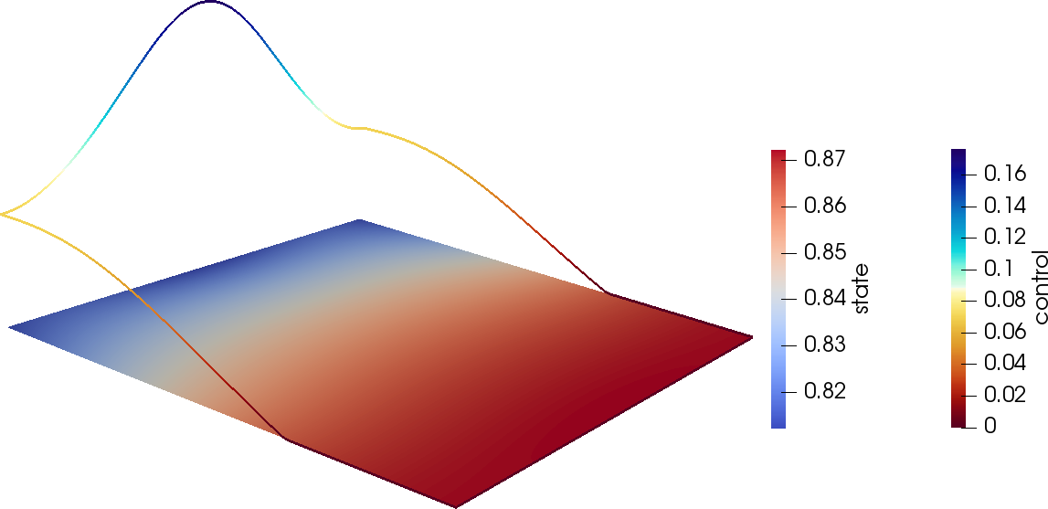
Figure 1: Optimal state (surface) and the optimal control (boundary curve) for the benchmark problem.

The optimal control and corresponding state of our benchmark problem is illustrated in Figure 1 and the measured discretization errors as well as the experimentally computed convergence rates are summarized in Table 1. As we have proven in Theorem 5.6 the numerical solutions obtained by a full discretization using a piecewise constant control approximation converge with the optimal convergence rate $1$. Moreover, it is confirmed that the solution obtained with a postprocessing step, see Theorem 5.11, converges with order $2$. Note that we actually proved the results for the case that the boundary is smooth which is indeed not the case in our example. However, the corner singularities contained in the solution are for a $90^{\circ}$-corner comparatively mild so that the regularity results from Lemma 3.10 remain valid.

$i$	DOF	BD DOF	$\|u-u_{h_{i}}\|_{L^{2}(\Gamma)}$ (eoc)	$\|u-\tilde{u}_{h_{i}}\|_{L^{2}(\Gamma)}$ (eoc)
$3$	113	32	1.60e-2 (1.06)	1.81e-2 (1.15)
$4$	353	64	5.81e-3 (1.46)	4.43e-3 (2.03)
$5$	1217	128	2.56e-3 (1.18)	1.03e-3 (2.11)
$6$	4481	256	1.24e-3 (1.05)	1.65e-4 (2.64)
$7$	17153	512	6.17e-4 (1.00)	7.52e-5 (1.13)
$8$	67073	1024	3.06e-4 (1.01)	1.79e-5 (2.07)
$9$	265217	2048	1.49e-4 (1.04)	4.31e-6 (2.05)
$10$	1054716	4096	6.67e-5 (1.16)	8.50e-7 (2.34)

Table 1: Experimentally computed errors for the full discretization and the postprocessing approach with the corresponding experimental convergence rates (in parentheses)

Appendix A Proof of Theorem 4.3

The proof of the maximum norm estimate presented in Theorem 4.3 follows basically from the arguments of [16, 34]. For the convenience of the reader we want to repeat the proof as the result of Theorem 4.3 is, for our specific situation, not directly available in the literature. The novelty of the present proof is that it includes curved elements as well as Robin boundary conditions. In the aforementioned articles, a representation of the error term based on a regularized Dirac function is used. This function forms the right-hand side of a dual problem whose solution is an approximation of Green’s function. The main difficulty is to bound this solution in appropriate norms.

To this end, we denote by $T^{*}\in\mathcal{T}_{h}$ the element where $|y-y_{h}|$ attains its maximum. The regularized Dirac function is defined by $\delta^{h}(x):=|T^{*}|^{-1}\operatorname{sgn}(y(x)-y_{h}(x))$ if $x\in T^{*}$, and $\delta^{h}(x):=0$ if $x\not\in T^{*}$. The corresponding Green’s function denoted by $g^{h}$ solves the problem

$$-\Delta g^{h}+g^{h}=\delta^{h}\quad\mbox{in}\quad\Omega,\qquad\partial_{n}g^{h}+u\,g^{h}=0\quad\mbox{on}\quad\Gamma.$$ (56)

The Dirac function satisfies the properties

$$\|\delta^{h}\|_{L^{1}(\Omega)}\leq c,\qquad\|\delta^{h}\|_{L^{2}(\Omega)}\leq c\,h^{-1}.$$ (57)

We start our considerations with some a priori estimates for the solution $g^{h}$.

Lemma A.1.

The following a priori estimates hold:

$$(i) \|g^{h}\|_{H^{1}(\Omega)} \leq c\,\lvert\ln h\rvert^{1/2} (ii) \|g^{h}\|_{H^{2}(\Omega)} \leq c\,h^{-1}$$

$$(iii) \|g^{h}\|_{L^{\infty}(\Omega)} \leq c\,\lvert\ln h\rvert$$

Proof.

(ii) To show the estimate in the $H^{2}(\Omega)$-norm we apply the a priori estimate from Lemma 2.3c) and $\|\delta^{h}\|_{L^{2}(\Omega)}\leq ch^{-1}$.
(i) The weak form of (56) and the property (57) imply

$$\gamma_{u}\,\|g^{h}\|_{H^{1}(\Omega)}^{2} \leq a_{u}(g^{h},g^{h})=(\delta^{h},g^{h})_{L^{2}(\Omega)}\leq c\,\|g^{h}\|_{L^{\infty}(\Omega)}$$

$$\leq c\left(\|g^{h}-g_{h}^{h}\|_{L^{\infty}(\Omega)}+\lvert\ln h\rvert^{1/2}\,\|g_{h}^{h}\|_{H^{1}(\Omega)}\right),$$ (58)

where the discrete Sobolev inequality was applied in the last step. The function $g_{h}^{h}\in V_{h}$ is the Ritz-projection of $g^{h}$ and satisfies the usual stability estimate

$$\|g_{h}^{h}\|_{H^{1}(\Omega)}\leq c\,\|g^{h}\|_{H^{1}(\Omega)}.$$ (59)

Next, we derive a suboptimal error estimate for the finite-element error in the $L^{\infty}(\Omega)$-norm. Using an inverse inequality, estimates for the interpolant $\Pi_{h}$ from (17), the Aubin-Nitsche trick and the a priori estimate shown already in the $H^{2}(\Omega)$-norm we deduce

$$\|g^{h}-g^{h}_{h}\|_{L^{\infty}(\Omega)} \leq\|g^{h}-\Pi_{h}g^{h}\|_{L^{\infty}(\Omega)}+c\,h^{-1}\left(\|g^{h}-\Pi_{h}g^{h}\|_{L^{2}(\Omega)}+\|g^{h}-g_{h}^{h}\|_{L^{2}(\Omega)}\right)$$

$$\leq c\,h\,\|g^{h}\|_{H^{2}(\Omega)}\leq c.$$ (60)

Note that we hide the dependency on $u$, or more precisely on $\|u\|_{H^{1/2}(\Omega)}$ and lower-order norms, in the generic constant to simplify the notation. Insertion of (59) and (A) into (A) yields with Young’s inequality

$$\gamma_{u}\,\|g^{h}\|_{H^{1}(\Omega)}^{2}\leq c\,\lvert\ln h\rvert+\frac{1}{2}\,\gamma_{u}\,\|g^{h}\|_{H^{1}(\Omega)}^{2}.$$

The desired estimate follows form a kick-back-argument.
(iii) The $L^{\infty}(\Omega)$-estimate follows directly from (A), (59) and (A) using the inequality (i). ∎

Next, we show an a priori estimate for $g^{h}$ in a weighted norm. This is the key idea which allows us to bound second derivatives by a logarithmic factor only. The weight function we will use is defined by

$$\sigma(x):=\sqrt{|x-x^{*}|_{2}^{2}+c\,h^{2}},$$

with $x^{*}:=\operatorname{arg\,max}_{x\in T^{*}}|y-y_{h}|(x)$. This function satisfies

$$\|\sigma^{-1}\|_{L^{2}(\Omega)}\leq c\,\lvert\ln h\rvert^{1/2},\qquad\|\sigma^{-1}\|_{L^{2}(\Gamma)}\leq c\,h^{-1/2}\,\lvert\ln h\rvert^{1/4}.$$ (61)

The first property follows from a simple computation. The second estimate is a consequence of the multiplicative trace theorem $\|\sigma^{-1}\|_{L^{2}(\Gamma)}\leq c\,\|\sigma^{-1}\|_{L^{2}(\Omega)}^{1/2}\,\|\sigma^{-1}\|_{H^{1}(\Omega)}^{1/2}$, see [6, Theorem 1.6.6], and the chain rule $\nabla\sigma^{-1}=-\sigma^{-2}\nabla\sigma$ and it is simple to show $\|\nabla\sigma\|_{L^{\infty}(\Omega)}\leq 1$ and $\|\sigma^{-2}\|_{L^{2}(\Omega)}\leq c\,h^{-1}$.

Lemma A.2.

Assume that $u\in H^{1/2}(\Gamma)$. There holds the estimate

$$\|\sigma\,\nabla^{2}g^{h}\|_{L^{2}(\Omega)}\leq c\,\lvert\ln h\rvert^{1/2}.$$

Proof.

We introduce the functions $\xi_{i}:=|x_{i}-x_{i}^{*}|$, $i=1,2$, which allow us to write

$$\|\sigma\,\nabla^{2}g^{h}\|_{L^{2}(\Omega)}^{2}=\sum_{i=1}^{2}\|\xi_{i}\,\nabla^{2}g^{h}\|_{L^{2}(\Omega)}^{2}+c\,h^{2}\,\|\nabla^{2}g^{h}\|_{L^{2}(\Omega)}^{2}.$$ (62)

With the reverse product rule we obtain

$$\|\xi_{i}\,\nabla^{2}g^{h}\|_{L^{2}(\Omega)}^{2}\leq\|\nabla^{2}(\xi_{i}\,g^{h})\|_{L^{2}(\Omega)}^{2}+\|\nabla g^{h}\|_{L^{2}(\Omega)}^{2}.$$ (63)

Moreover, we easily confirm that $\xi_{i}\,g^{h}$ is the solution of the problem

$$-\Delta(\xi_{i}\,g^{h})+\xi_{i}\,g^{h} =-2\,\frac{\partial g^{h}}{\partial x_{i}}+\xi_{i}\,\delta^{h} \mbox{in}\ \Omega,$$

$$\partial_{n}(\xi_{i}\,g^{h})+u\,\xi_{i}\,g^{h} =g^{h}\,n_{i} \mbox{on}\ \Gamma,$$

where $n_{i}$ is the $i$-th component of the outer unit normal vector on $\Gamma$. Lemma 2.3c) using the property $\|\xi_{i}\,\delta^{h}\|_{L^{2}(\Omega)}\leq c$, which follows from a simple computation, leads to

$$\|\nabla^{2}(\xi_{i}\,g^{h})\|_{L^{2}(\Omega)} \leq c\left(1+\|u\|_{H^{1/2}(\Gamma)}\right)\left(1+\|\nabla g^{h}\|_{L^{2}(\Omega)}+\|g^{h}\|_{H^{1/2}(\Gamma)}\right)$$

$$\leq c\left(1+\|g^{h}\|_{H^{1}(\Omega)}\right).$$ (64)

Insertion into (63) and using Lemma A.1(i) leads to

$$\|\xi_{i}\,\nabla^{2}g^{h}\|_{L^{2}(\Omega)}\leq c\,\lvert\ln h\rvert^{1/2},\quad i=1,2.$$

An estimate for the second term on the right-hand side of (62) is derived in Lemma A.1(ii). ∎

Next, we derive some error estimates for the approximation $g_{h}^{h}$ in several norms.

Lemma A.3.

Assume that $u\in H^{1/2}(\Gamma)$. Then, there hold the error estimates

$$h^{-1}\,\|g^{h}-g_{h}^{h}\|_{L^{2}(\Omega)}+\|\nabla(g^{h}-g_{h}^{h})\|_{L^{2}(\Omega)} \leq c,$$

$$\|\sigma\nabla^{2}(g^{h}-g_{h}^{h})\|_{L^{2}_{\textup{pw}}(\Omega)} \leq c\,\lvert\ln h\rvert^{1/2}.$$

Proof.

The first estimate follows directly from the $H^{1}(\Omega)$-error estimate stated in Lemma 4.1 and the Aubin-Nitsche trick. Moreover, the a priori estimate for the $H^{2}(\Omega)$-norm of $g^{h}$ from Lemma A.1 has to be exploited.

In the second estimate one observes that the discrete function $g_{h}^{h}$ would vanish except on curved elements (note that $g_{h}^{h}$ is affine on the reference element only, but not on $T$). With the transformation result [5, Lemma 2.3] we obtain

$$\|\nabla^{2}(g^{h}-g_{h}^{h})\|_{L^{2}(T)} \leq\,c\,|T|^{1/2}\,h^{-2}\sum_{k=0}^{2}h^{4-2k}\,\|\hat{\nabla}^{k}(\hat{g}^{h}-\hat{g}_{h}^{h})\|_{L^{2}(\hat{T})}$$

$$\leq c\left(\|\nabla^{2}g^{h}\|_{L^{2}(T)}+h\,\|g^{h}-g_{h}^{h}\|_{H^{1}(T)}\right),$$

where $g^{h}=\hat{g}^{h}\circ F_{T}^{-1}$, $g_{h}^{h}=\hat{g}_{h}^{h}\circ F_{T}^{-1}$. Taking into account $\inf_{x\in T}\sigma(x)\sim\sup_{x\in T}\sigma(x)$, which holds due to the assumed shape-regularity, and $|\sigma(x)|\leq c$ for all $x\in\Omega$, we obtain

$$\|\sigma\,\nabla^{2}(g^{h}-g_{h}^{h})\|_{L^{2}_{\textup{pw}}(\Omega)}\leq c\left(\|\sigma\,\nabla^{2}g^{h}\|_{L^{2}(\Omega)}+h\,\|g^{h}-g_{h}^{h}\|_{H^{1}(\Omega)}\right).$$

The first term has been discussed in the previous Lemma and the last term has been considered in the present Lemma already. ∎

Now we are in the position to prove Theorem 4.3.

Proof.

With an inverse inequality and the Hölder inequality, the definition of $\delta^{h}$ and a maximum norm estimate for the interpolant $\Pi_{h}$, see e. g. [5, Theorem 4.1], we obtain

$$\|y-y_{h}\|_{L^{\infty}(\Omega)}=\|y-y_{h}\|_{L^{\infty}(T^{*})} \leq c\left(\|y-\Pi_{h}y\|_{L^{\infty}(T^{*})}+|T^{*}|^{-1}\,\|\Pi_{h}y-y_{h}\|_{L^{1}(T^{*})}\right)$$

$$\leq c\left(\|y-\Pi_{h}y\|_{L^{\infty}(T^{*})}+(\delta^{h},y-y_{h})_{L^{2}(\Omega)}\right)$$

$$\leq c\left(h^{2-2/q}\,\|y\|_{W^{2,q}(\Omega)}+a_{u}(y-y_{h},g^{h})\right),$$ (65)

where $g_{h}^{h}\in V_{h}$ denotes the Ritz projection of $g^{h}$.

For the latter part on the right-hand side of (A) we get with the Galerkin orthogonality, the Hölder inequality, a trace theorem for the boundary integral term as well as $\|u\|_{L^{\infty}(\Gamma)}\leq c$

$$a_{u}(y-y_{h},g^{h})=a_{u}(y-\Pi_{h}y,g^{h}-g_{h}^{h})$$

$$\quad\leq c\,\|y-\Pi_{h}y\|_{W^{1,\infty}(\Omega)}\,\|g^{h}-g_{h}^{h}\|_{W^{1,1}(\Omega)}.$$ (66)

An estimate for the interpolation error is deduced in [5]. The $L^{1}(\Omega)$-norms can be replaced by weighted $L^{2}(\Omega)$-norms involving the weighting function $\sigma$. Taking into account the properties (61) we obtain

$$\|g^{h}-g_{h}^{h}\|_{W^{1,1}(\Omega)}\leq c\,\lvert\ln h\rvert^{1/2}\,\left(\|\sigma\,\nabla(g^{h}-g_{h}^{h})\|_{L^{2}(\Omega)}+\|g^{h}-g_{h}^{h}\|_{L^{2}(\Omega)}\right).$$ (67)

In the following we will show that the expressions on the right-hand side of (67) are bounded by $c\,h\,\lvert\ln h\rvert^{1/2}$. Therefore, we apply the reverse product rule and get

$$\|\sigma\,\nabla(g^{h}-g_{h}^{h})\|_{L^{2}(\Omega)}^{2}$$

$$\qquad=(\nabla(\sigma^{2}\,(g^{h}-g_{h}^{h})),\nabla(g^{h}-g_{h}^{h}))_{L^{2}(\Omega)}-((g^{h}-g_{h}^{h})\,\nabla\sigma^{2},\nabla(g^{h}-g_{h}^{h}))_{L^{2}(\Omega)}.$$

From this we conclude

$$\Theta^{2}:=\|\sigma\nabla(g^{h}-g_{h}^{h})\|_{L^{2}(\Omega)}^{2}+\|g^{h}-g_{h}^{h}\|_{L^{2}(\Omega)}^{2}$$

$$\qquad\leq a_{u}(\sigma^{2}(g^{h}-g_{h}^{h}),g^{h}-g_{h}^{h})-((g^{h}-g_{h}^{h})\nabla\sigma^{2},\nabla(g^{h}-g_{h}^{h}))_{L^{2}(\Omega)}.$$ (68)

Here, we exploited that $(u\,\sigma^{2}\,(g^{h}-g_{h}^{h}),g^{h}-g_{h}^{h})_{L^{2}(\Gamma)}\geq 0$ due to $u\geq u_{a}\geq 0$. Next, we introduce the abbreviation $z:=\sigma^{2}\,(g^{h}-g_{h}^{h})$. The Galerkin orthogonality of $g^{h}-g_{h}^{h}$, Young’s inequality and the trace theorem taking into account $|\sigma|+|\nabla\sigma|\leq c$ yield

$$\|\sigma\,v\|_{L^{2}(\Gamma)}\leq c\left(\|\sigma\,v\|_{L^{2}(\Omega)}+\|\nabla(\sigma\,v)\|_{L^{2}(\Omega)}\right)\leq c\left(\|v\|_{L^{2}(\Omega)}+\|\sigma\,\nabla v\|_{L^{2}(\Omega)}\right)$$

and thus,

$$a_{u}(\sigma^{2}(g^{h}-g_{h}^{h}),g^{h}-g_{h}^{h})=a_{u}(z-\Pi_{h}z,g^{h}-g_{h}^{h})$$

$$\qquad\leq\frac{1}{4}\,\Theta^{2}+c\,\Big{(}\|\sigma^{-1}\,\nabla(z-\Pi_{h}z)\|_{L^{2}(\Omega)}^{2}$$

$$\qquad\phantom{\frac{1}{2}\Theta^{2}+c\leq}+\|\sigma^{-1}\,(z-\Pi_{h}z)\|_{L^{2}(\Omega)}^{2}+\|\sigma^{-1}\,u\,(z-\Pi_{h}z)\|_{L^{2}(\Gamma)}^{2}\Big{)}.$$ (69)

Next, we derive local interpolation error estimates. In the following we use the notation $\underline{\sigma}_{T}:=\inf_{x\in T}\sigma(x)$ and $\overline{\sigma}_{T}:=\sup_{x\in T}\sigma(x)$. Due to the assumed shape-regularity there holds $\underline{\sigma}_{T}\sim\overline{\sigma}_{T}$ for all $T\in\mathcal{T}_{h}$, and hence,

$$\|\sigma^{-1}\,\nabla(z-\Pi_{h}z)\|_{L^{2}(T)}+h^{-1}\,\|\sigma^{-1}\,(z-\Pi_{h}z)\|_{L^{2}(T)}\leq c\,\underline{\sigma}_{T}^{-1}\,h\,\|\sigma^{2}\,(g^{h}-g_{h}^{h})\|_{H^{2}(\tilde{T})},$$

where $\tilde{T}$ is the patch of all elements adjacent to $T$ (note that $\Pi_{h}$ is a quasi-interpolant). The Leibniz rule and the properties $|\nabla\sigma^{2}|\leq\sigma$ and $|\nabla^{2}\sigma^{2}|\leq c$ imply

$$\|\sigma^{2}\,(g^{h}-g_{h}^{h})\|_{H^{2}(\tilde{T})}\leq\|g^{h}-g_{h}^{h}\|_{L^{2}(\tilde{T})}+\|\sigma\,\nabla(g^{h}-g_{h}^{h})\|_{L^{2}(\tilde{T})}+\|\sigma^{2}\,\nabla^{2}(g^{h}-g_{h}^{h})\|_{L^{2}(\tilde{T})}.$$

Next, we combine the two estimates above and take into account the properties $h\,\underline{\sigma}_{T}^{-1}\leq c$ and $\overline{\sigma}_{T}\sim\overline{\sigma}_{\tilde{T}}$ which follows from the assumed quasi-uniformity. Summation over all $T\in\mathcal{T}_{h}$ and an application of Lemma A.3 yields

$$\|\sigma^{-1}\nabla(z-\Pi_{h}z)\|_{L^{2}(\Omega)}+h^{-1}\,\|\sigma^{-1}(z-\Pi_{h}z)\|_{L^{2}(\Omega)}$$

$$\quad\leq c\left(\|g^{h}-g_{h}^{h}\|_{L^{2}(\Omega)}+h\,\|\nabla(g^{h}-g_{h}^{h})\|_{L^{2}(\Omega)}+h\,\|\sigma\,\nabla^{2}(g^{h}-g_{h}^{h})\|_{L^{2}_{\textup{pw}}(\Omega)}\right)$$

$$\quad\leq c\,h\,\lvert\ln h\rvert^{1/2}.$$ (70)

It remains to discuss the third term on the right-hand side of (A). With interpolation error estimates for $\Pi_{h}$ on the boundary, compare also (18), and $u\in L^{\infty}(\Gamma)$ we obtain

$$\|\sigma^{-1}\,u\,(z-\Pi_{h}z)\|_{L^{2}(E)} \leq c\,h\,\underline{\sigma}_{E}^{-1}\|\nabla z\|_{L^{2}(\tilde{E})}$$

$$\leq c\,h\left(\|g^{h}-g_{h}^{h}\|_{L^{2}(E)}+\|\sigma\,\nabla(g^{h}-g_{h}^{h})\|_{L^{2}(\tilde{E})}\right),$$ (71)

where we exploited the product rule and the property $\nabla\sigma^{2}\leq 2\sigma\vec{1}$ in the last step. With a trace theorem and Lemma A.3 we conclude

$$\|g^{h}-g_{h}^{h}\|_{L^{2}(\Gamma)}\leq c\,\|g^{h}-g_{h}^{h}\|_{H^{1}(\Omega)}\leq c,$$

and with a multiplicative trace theorem, Young’s inequality, the product rule and the estimates from Lemma A.3 we obtain

$$\|\sigma\,\nabla(g^{h}-g_{h}^{h})\|_{L^{2}(\Gamma)} \leq c\left(\|\sigma\,\nabla(g^{h}-g_{h}^{h})\|_{L^{2}(\Omega)}+\|\nabla(\sigma\,\nabla(g^{h}-g_{h}^{h}))\|_{L_{\textup{pw}}^{2}(\Omega)}\right)$$

$$\leq c\left(\|\nabla(g^{h}-g_{h}^{h}))\|_{L^{2}(\Omega)}+\|\sigma\,\nabla^{2}(g^{h}-g_{h}^{h})\|_{L_{\textup{pw}}^{2}(\Omega)}\right)$$

$$\leq c\,\lvert\ln h\rvert^{1/2}.$$

The estimate (A) then simplifies to

$$\|\sigma^{-1}\,(z-\Pi_{h}z)\|_{L^{2}(\Gamma)}\leq c\,h\,\lvert\ln h\rvert^{1/2}.$$ (72)

Insertion of (A) and (72) into (A) leads to the estimate

$$a(\sigma^{2}(g^{h}-g_{h}^{h}),g^{h}-g_{h}^{h})\leq\frac{1}{4}\Theta^{2}+c\,h^{2}\,\lvert\ln h\rvert.$$ (73)

It remains to show an estimate for the second term on the right-hand side of (A). Due to $|\nabla\sigma^{2}|\leq 2\sigma\vec{1}$, Young’s inequality and the $L^{2}(\Omega)$-error estimate from Lemma A.3 we get

$$((g^{h}-g_{h}^{h})\nabla\sigma^{2},\nabla(g^{h}-g_{h}^{h}))_{L^{2}(\Omega)} \leq c\,\|g^{h}-g_{h}^{h}\|_{L^{2}(\Omega)}^{2}+\frac{1}{4}\,\|\sigma\,\nabla(g^{h}-g_{h}^{h})\|_{L^{2}(\Omega)}^{2}$$

$$\leq c\,h^{2}+\frac{1}{4}\,\Theta^{2}.$$ (74)

Insertion of (73) and (A) into (A) yields

$$\Theta^{2}\leq\frac{1}{2}\,\Theta^{2}+c\,h^{2}\,\lvert\ln h\rvert$$ (75)

and with a kick-back-argument we conclude $\Theta^{2}=c\,h^{2}\,\lvert\ln h\rvert$. Finally, we collect up the previous estimates. To this end, we insert (75) into (67), the resulting estimate into (A) and this into (A). ∎

Appendix B Local estimates for the midpoint interpolant and the $L^{2}(\Gamma)$-projection

To the best of the author’s knowledge there are no error estimates for the midpoint interpolant defined on a curved boundary available in the literature. Thus, we prove the following Lemmata which are needed in the proof of Lemma 5.9.

Consider a single boundary element $E\subset\bar{T}$ with corresponding element $T\in\mathcal{T}_{h}$. A parametrization of the boundary element is given by $E:=\{\gamma_{E}(\xi):=F_{T}(\xi,0),\ \xi\in(0,1)\}$ when assuming that the edge of $\hat{T}$ with endpoints $(0,0)$, $(1,0)$ is mapped onto $E$. In the following we denote the length of a boundary element $E\in\mathcal{E}_{h}$ by $L_{E}=\int_{0}^{1}|\dot{\gamma}_{E}(\xi)|\,\mathrm{d}\xi$.

Lemma B.1.

For each function $u\colon\Gamma\to\mathbb{R}$ there exists some piecewise constant function $R_{h}u\in U_{h}$ satisfying the local estimates

$$\left|\int_{E}(u-R_{h}u)\right| \leq c\,h^{5/2}\left(\|\nabla u\|_{L^{2}(E)}+\|\nabla^{2}u\|_{L^{2}(E)}\right),$$

$$\|u-R_{h}u\|_{L^{\infty}(E)} \leq c\,h^{1-1/q}\,\|\nabla u\|_{L^{q}(E)},\quad q\in(1,\infty],$$

for all $E\in\mathcal{E}_{h}$, provided that $u$ possesses the regularity demanded by the right-hand side.

Proof.

Let us first construct a suitable interpolation operator. To obtain the desired second-order accuracy we have to guarantee that the property $\int_{E}p=\int_{E}R_{h}p$ holds for all functions $p(\gamma_{E}(\xi))=\hat{p}(\xi)$ with some first-order polynomial $\hat{p}(\xi):=a+b\,\xi$. The transformation to $\hat{E}:=(0,1)\times\{0\}$ yields

$$\int_{E}(p(x)-R_{h}p)\mathrm{d}s_{x}=\int_{0}^{1}(\hat{p}(\xi)-\hat{p}(\xi_{E}))\,|\dot{\gamma}_{E}(\xi)|\,\mathrm{d}\xi=b\,\int_{0}^{1}(\xi-\xi_{E})\,|\dot{\gamma}_{E}(\xi)|\,\mathrm{d}\xi=0.$$

The latter step holds true when choosing

$$\xi_{E}:=\frac{1}{L_{E}}\int_{0}^{1}\xi\,|\dot{\gamma}_{E}(\xi)|\,\mathrm{d}\xi$$

To this end, we define our operator by means of $R_{h}u|_{E}=\hat{u}(\xi_{E})$. Obviously, the definition of $R_{h}$ depends on the transformations $F_{T}$.

To show the interpolation error estimates we apply the property $\int_{E}(p-R_{h}p)=0$ for arbitrary $p\in\mathcal{P}_{1}$, the stability of the interpolant $\hat{R}_{h}\hat{u}|_{E}=\hat{u}(\xi_{E})$, the properties (16) of the transformation $F_{T}$ and the Bramble-Hilbert Lemma. This yields

$$\int_{E}(u(x)-R_{h}u)\mathrm{d}s_{x} =\int_{0}^{1}(I-\hat{R}_{h})(\hat{u}-\hat{p})(\xi)\,|\dot{\gamma}_{E}(\xi)|\,\mathrm{d}\xi$$

$$\leq c\,h\,\|\hat{u}-\hat{p}\|_{L^{\infty}(\hat{E})}\leq c\,h\,\|\partial_{\xi\xi}\hat{u}\|_{L^{2}(\hat{E})}.$$

For the transformation back to the world element $E$ we apply the chain rule

$$\partial_{\xi\xi}\hat{u}(\xi)=\dot{\gamma}_{E}(\xi)^{\top}\,\nabla^{2}u(\gamma_{E}(\xi))\,\dot{\gamma}_{E}(\xi)+\ddot{\gamma}_{E}(\xi)^{\top}\,\nabla u(\gamma_{E}(\xi))$$

and the properties (16) to arrive at

$$\|\partial_{\xi\xi}\hat{u}\|_{L^{2}(\hat{E})} \leq c\,h^{2}\left(\max_{\xi}|\dot{\gamma}_{E}(\xi)|^{-1}\sum_{|\alpha|=1}^{2}\int_{0}^{1}(D^{\alpha}u(\gamma_{E}(\xi)))^{2}\,|\dot{\gamma}_{E}(\xi)|\,\mathrm{d}\xi\right)^{1/2}$$

$$\leq c\,h^{2}\left(\min_{\xi}|\dot{\gamma}_{E}(\xi)|\right)^{-1/2}\left(\|\nabla u\|_{L^{2}(E)}+\|\nabla^{2}u\|_{L^{2}(E)}\right).$$

Finally, the norm of $\dot{\gamma}_{E}$ can be bounded by means of

$$|\dot{\gamma}_{E}(\xi)|^{-1}=|DF_{T}(\xi,0)(1,\,0)^{\top}|^{-1}\leq\left(\min_{\|x\|=1}|DF_{T}(\xi,0)x|\right)^{-1}=\|DF_{T}(\xi,0)^{-1}\|.$$ (76)

Note, that the last step is valid for the spectral norm only. An application of Lemma 2.2 from [5] which provides $\sup_{\hat{x}\in\hat{T}}\|DF_{T}(\hat{x})^{-1}\|\leq ch^{-1}$ leads to the first estimate.

The second estimate follows with similar arguments. For an arbitrary constant $\hat{p}$ we then obtain

$$\|u-R_{h}u\|_{L^{\infty}(E)}\leq\|(I-\hat{R}_{h})(\hat{u}-\hat{p})\|_{L^{\infty}(\hat{E})}\leq c\,|\hat{u}|_{W^{1,q}(\hat{E})}\leq c\,h\,|E|^{-1/q}\,\|\nabla u\|_{L^{q}(E)}.$$

∎

A further operator that is needed in Section 3 is the $L^{2}(\Gamma)$-projection onto $U_{h}$. In case of curved boundaries, this operator reads

$$[Q_{h}v]|_{E}:=\frac{1}{L_{E}}\int_{0}^{1}v(\gamma_{E}(\xi))\,|\dot{\gamma}_{E}(\xi)|\,\mathrm{d}\xi$$

for each $E\in\mathcal{E}_{h}$. Note that this definition implies the orthogonality property

$$(u-Q_{h}u,v_{h})_{L^{2}(\Gamma)}=0\qquad\forall v_{h}\in U_{h}.$$ (77)

With similar arguments as in the previous Lemma we obtain the following local estimate which is standard in case of a boundary consisting of straight edges.

Lemma B.2.

Assume that $u\in H^{1}(\Gamma)$. Then the estimate

$$\|u-Q_{h}u\|_{L^{2}(E)}\leq c\,h\,\|\nabla u\|_{L^{2}(E)}$$

is fulfilled for all $E\in\mathcal{E}_{h}$.

Proof.

We introduce a further projection onto $U_{h}$, namely $[\tilde{Q}_{h}u]|_{E}:=\int_{0}^{1}u(\gamma_{E}(\xi))\,\mathrm{d}\xi$. Using (77), the transformation to the reference element as in the previous Lemma and the Poincaré inequality we obtain

$$\|u-Q_{h}u\|_{L^{2}(E)}^{2} \leq\|u-\tilde{Q}_{h}u\|_{L^{2}(E)}^{2}$$

$$=\int_{0}^{1}\left(u(\gamma_{E}(\xi))-\int_{0}^{1}u(\gamma_{E}(\xi^{\prime}))\,\mathrm{d}\xi^{\prime}\right)^{2}|\dot{\gamma}_{E}(\xi)|\,\mathrm{d}\xi$$

$$\leq c\,h\,\|\partial_{\xi}u(\gamma_{E}(\cdot))\|_{L^{2}(0,1)}^{2}\leq c\,h^{2}\,\|\nabla u\|_{L^{2}(E)}^{2}$$

where the last step is a consequence of the chain rule $\partial_{\xi}u(\gamma_{E}(\xi))=\nabla u(\gamma_{E}(\xi))\cdot\dot{\gamma}_{E}(\xi)$ and $|\dot{\gamma}_{E}(\xi)|\sim h$ for all $\xi\in(0,1)$, see also (76). ∎

We conclude this section with an estimate for an expression which is need in Lemma 5.9.

Lemma B.3.

Assume that the functions $u$ and $v$ belong to $\in H^{1}(\Gamma)$. Then the inequality

$$(u-R_{h}u,v)_{L^{2}(\Gamma)}\leq c\,h^{2}\,\|\nabla u\|_{L^{2}(\Gamma)}\,\|\nabla v\|_{L^{2}(\Gamma)}+c\,\|v\|_{L^{\infty}(\Gamma)}\sum_{E\in\mathcal{E}_{h}}\left|\int_{E}(u-R_{h}u)\right|$$

is valid.

Proof.

First, we split the term under consideration using the $L^{2}(\Gamma)$-projection onto $U_{h}$ and obtain

$$(u-R_{h}u,v)_{L^{2}(\Gamma)}=(u-Q_{h}u,v-Q_{h}v)_{L^{2}(\Gamma)}+(Q_{h}(u-R_{h}u),v)_{L^{2}(\Gamma)}.$$

The first term on the right-hand side can be treated with the local estimate from Lemma B.2 which yields

$$(u-Q_{h}u,v-Q_{h}v)_{L^{2}(\Gamma)}\leq c\,h^{2}\,\|\nabla u\|_{L^{2}(\Gamma)}\,\|\nabla v\|_{L^{2}(\Gamma)}.$$

For the second term we exploit the definition of $Q_{h}$ and $R_{h}$ on the reference element. For each $E\in\mathcal{E}_{h}$ we then obtain

$$\|Q_{h}(u-R_{h}u)\|_{L^{1}(E)} =\int_{0}^{1}\left|\frac{1}{L_{E}}\int_{0}^{1}(u(\gamma_{E}(\xi))-u(\gamma_{E}(\xi_{E})))\,|\dot{\gamma}_{E}(\xi)|\,\mathrm{d}\xi\right|\,|\dot{\gamma}_{E}(\xi^{\prime})|\,\mathrm{d}\xi^{\prime}$$

$$=\left|\int_{0}^{1}(u(\gamma_{E}(\xi))-u(\gamma_{E}(\xi_{E})))\,|\dot{\gamma}_{E}(\xi)|\,\mathrm{d}\xi\right|=\left|\int_{E}(u-R_{h}u)\right|,$$

where we used $\int_{0}^{1}|\dot{\gamma}_{E}(\xi^{\prime})|\,\mathrm{d}\xi^{\prime}=L_{E}$ in the second step. Consequently, we obtain

$$(Q_{h}(u-R_{h}u),v)_{L^{2}(\Gamma)}\leq c\,\|v\|_{L^{\infty}(\Gamma)}\sum_{E\in\mathcal{E}_{h}}\left|\int_{E}(u-R_{h}u)\right|$$

and conclude the assertion. ∎

References

• [1] Th. Apel “Anisotropic finite elements: Local estimates and applications.” Stuttgart: Teubner, 1999
• [2] Th. Apel, J. Pfefferer and A. Rösch “Finite element error estimates on the boundary with application to optimal control” In Math. Comp. 84, 2015, pp. 33–70 DOI: 10.1090/S0025-5718-2014-02862-7
• [3] Th. Apel, J. Pfefferer and M. Winkler “Error estimates for the postprocessing approach applied to Neumann boundary control problems in polyhedral domains” In IMA Journal of Numerical Analysis 38.4, 2018, pp. 1984–2025 DOI: 10.1093/imanum/drx059
• [4] N. Arada, E. Casas and F. Tröltzsch “Error estimates for the numerical approximation of a semilinear elliptic control problem.” In Comput. Optim. Appl. 23.2 Springer US, New York, NY, 2002, pp. 201–229 DOI: 10.1023/A:1020576801966
• [5] C. Bernardi “Optimal finite-element interpolation on curved domains.” In SIAM J. Numer. Anal. 26.5 Society for IndustrialApplied Mathematics (SIAM), Philadelphia, PA, 1989, pp. 1212–1240 DOI: 10.1137/0726068
• [6] S.. Brenner and L.. Scott “The mathematical theory of finite element methods.”, Texts in applied mathematics Springer, New York, 2008
• [7] E. Casas “Boundary control of semilinear elliptic equations with pointwise state constraints.” In SIAM J. Control Optim. 31.4 Society for IndustrialApplied Mathematics (SIAM), Philadelphia, PA, 1993, pp. 993–1006 DOI: 10.1137/0331044
• [8] E. Casas and M. Mateos “Error estimates for the numerical approximation of Neumann control problems.” In Comput. Optim. Appl. 39.3, 2008, pp. 265–295 DOI: 10.1007/s10589-007-9056-6
• [9] E. Casas and M. Mateos “Uniform convergence of the FEM. Applications to state constrained control problems.” In Comput. Appl. Math. 21.1 Springer, Berlin/Heidelberg; Sociedade Brasileira de Matemática Aplicada e Computacional (SBMAC), São Carlos, 2002, pp. 67–100
• [10] E. Casas, M. Mateos and F. Tröltzsch “Error Estimates for the Numerical Approximation of Boundary Semilinear Elliptic Control Problems” In Comput. Optim. Appl. 31.2 Springer, 2005, pp. 193–219 DOI: 10.1007/s10589-005-2180-2
• [11] S. Chaabane and M. Jaoua “Identification of Robin coefficients by the means of boundary measurements” In Inverse Problems 15.6, 1999, pp. 1425–1438
• [12] P.. Ciarlet “Basic Error Estimates for Elliptic Problems.” In Finite Element Methods 2, Handbook of Numerical Analysis Elsevier, North-Holland, 1991, pp. 17–352
• [13] M. Dauge “Elliptic boundary value problems on corner domains.” Springer, Berlin, 1988 DOI: 10.1007/BFb0086682
• [14] V. Dhamo “Optimal boundary control of quasilinear elliptic partial differential equations: theory and numerical analysis”, 2012
• [15] K. Fellner, S. Rosenberger and B.. Tang “Quasi-steady-state approximation and numerical simulation for a volume-surface reaction-diffusion system” In Commun. Math. Sci. 14.6 International Press of Boston, 2016, pp. 1553–1580 DOI: 10.4310/cms.2016.v14.n6.a5
• [16] J. Frehse and R. Rannacher “Eine $L^{1}$-Fehlerabschätzung für diskrete Grundlösungen in der Methode der finiten Elemente.” In Bonn. Math. Schr. 89, 1976, pp. 92–114
• [17] F. Gesztesy and M. Mitrea “A description of all self-adjoint extensions of the Laplacian and Krein-type resolvent formulas on non-smooth domains.” In J. Anal. Math. 113, 2011, pp. 53–172 DOI: 10.1007/s11854-011-0002-2
• [18] P. Grisvard “Elliptic problems in nonsmooth domains” Pitman, Boston, 1985
• [19] J. Gwinner “On two-coefficient identification in elliptic variational inequalities” In Optimization 67.7 Informa UK Limited, 2018, pp. 1017–1030 DOI: 10.1080/02331934.2018.1446955
• [20] D.. Hào, P.. Thanh and D. Lesnic “Determination of the heat transfer coefficients in transient heat conduction” In IOP Inverse Problems 29.9, 2013 DOI: 10.1088/0266-5611/29/9/095020
• [21] E. Hetmaniok, J. Hristov, D. Słota and A. Zielonka “Identification of the heat transfer coefficient in the two-dimensional model of binary alloy solidification” In Heat and Mass Transfer 53.5, 2017, pp. 1657–1666 DOI: 10.1007/s00231-016-1923-1
• [22] M. Hinze “A variational discretization concept in control constrained optimization: the linear-quadratic case.” In Comput. Optim. Appl. 30.1 Norwell, MA, USA: Kluwer Academic Publishers, 2005, pp. 45–61 DOI: 10.1007/s10589-005-4559-5
• [23] B. Jin and X. Lu “Numerical identification of a Robin coefficient in parabolic problems.” In Math. Comp. 81.279 American Mathematical Society (AMS), Providence, RI, 2012, pp. 1369–1398 DOI: 10.1090/S0025-5718-2012-02559-2
• [24] D. Kinderlehrer and G. Stampacchia “An introduction to variational inequalities and their applications” 88, Pure and Applied Mathematics Academic Press, New York, 1980
• [25] A. Kröner and B. Vexler “A priori error estimates for elliptic optimal control problems with a bilinear state equation.” In J. Comput. Appl. Math. 230.2 Elsevier (North-Holland), Amsterdam, 2009, pp. 781–802 DOI: 10.1016/j.cam.2009.01.023
• [26] K. Krumbiegel and J. Pfefferer “Superconvergence for Neumann boundary control problems governed by semilinear elliptic equations” In Comput. Optim. Appl. 61.2, 2015, pp. 373–408 DOI: 10.1007/s10589-014-9718-0
• [27] J. Liu and G. Nakamura “Recovering the boundary corrosion from electrical potential distribution using partial boundary data” In Inverse Problems and Imaging 11.3 American Institute of Mathematical Sciences (AIMS), 2017, pp. 521–538 DOI: 10.3934/ipi.2017024
• [28] M. Mateos and A. Rösch “On saturation effects in the Neumann boundary control of elliptic optimal control problems.” In Comput. Optim. Appl. 49.2, 2011, pp. 359–378 DOI: 10.1007/s10589-009-9299-5
• [29] C. Meyer and A. Rösch “Superconvergence properties of optimal control problems.” In SIAM J. Control Optim. 43.3 Society for IndustrialApplied Mathematics, 2004, pp. 970–985 DOI: 10.1137/S0363012903431608
• [30] F. Mohebbi and M. Sellier “Identification of space- and temperature-dependent heat transfer coefficient” In International Journal of Thermal Sciences 128 Elsevier BV, 2018, pp. 28–37 DOI: 10.1016/j.ijthermalsci.2018.02.007
• [31] A. Rösch and F. Tröltzsch “An optimal control problem arising from the identification of nonlinear heat transfer laws” In Polish Academy of Sciences. Committee of Automatic Control and Robotics. Archives of Control Sciences 1.3-4, 1992, pp. 183–195
• [32] L.. Scott and S. Zhang “Finite element interpolation of nonsmooth functions satisfying boundary conditions.” In Math. Comp. 54.190, 1990, pp. 483–493 DOI: 10.2307/2008497
• [33] R. Scott “Finite Element Techniques for Curved Boundaries”, 1973
• [34] R. Scott “Optimal $L^{\infty}$ estimates for the finite element method on irregular meshes.” In Math. Comp. 30 American Mathematical Society (AMS), Providence, RI, 1976, pp. 681–697 DOI: 10.2307/2005390
• [35] G. Winkler “Control constrained optimal control problems in non-convex three dimensional polyhedral domains.”, 2008
• [36] M. Zlamal “Curved elements in the finite element method. I.” In SIAM J. Numer. Anal. 10, 1973, pp. 229–240 DOI: 10.1137/0710022