Classification of Legendrian knots of topological type $7_{6}$ with maximal Thurston–Bennequin number

Abstract.

We classify Legendrian knots of topological type $7_{6}$ having maximal Thurston–Bennequin number confirming the corresponding conjectures of [1].

This paper provides yet another illustration of the method of [5] for distinguishing Legendrian knots. The reader is referred to [5] for terminology.

If $R$ is a(n oriented) rectangular diagram of a knot, then by exchange class of $R$ denoted $\mathscr{E}(R)$ we mean the set of all (oriented) rectangular diagrams obtained from $R$ by exchange moves.

We use the notation of [3] for oriented types of stabilizations and destabilizations: $\overrightarrow{\mathrm{I}}$, $\overrightarrow{\mathrm{II}}$, $\overleftarrow{\mathrm{I}}$, and $\overleftarrow{\mathrm{II}}$. The following table shows the correspondence with the notation of [8]:

notation of [3] $\overrightarrow{\mathrm{I}}$ $\overleftarrow{\mathrm{I}}$ $\overrightarrow{\mathrm{II}}$ $\overleftarrow{\mathrm{II}}$ notation of [8] X:NE, O:SW X:SW, O:NE X:SE, O:NW X:NW, O:SE

A diagram obtained from $R$ by a stabilization of type $T$, where $T\in\bigl{\{}\overrightarrow{\mathrm{I}},\overrightarrow{\mathrm{II}},\overleftarrow{\mathrm{I}},\overleftarrow{\mathrm{II}}\bigr{\}}$, is denoted by $S_{T}(R)$. One can see that $\mathscr{E}(R_{1})=\mathscr{E}(R_{2})$ implies $\mathscr{E}\bigl{(}S_{T}(R_{1})\bigr{)}=\mathscr{E}\bigl{(}S_{T}(R_{2})\bigr{)}$ (this applies only to knots; in the case of many-component links, one should pay attention to which connected components of the diagrams are modified by the stabilizations). So, if $E$ is an exchange class of oriented rectangular diagrams of a knot and $R\in E$, then $S_{T}(E)=\mathscr{E}\bigl{(}S_{T}(R)\bigr{)}$ is a well defined exchange class not depending on the concrete choice of $R$.

By $\xi_{+}$ we denote the standard contact structure in $\mathbb{R}^{3}$, and by $\xi_{-}$ the mirror image of $\xi_{+}$:

$$\xi_{+}=\ker(x\,dy+dz),\quad\xi_{-}=\ker(x\,dy-dz).$$

By $\mathscr{L}_{+}(R)$ (respectively, $\mathscr{L}_{-}(R)$) we denote the equivalence class of $\xi_{+}$-Legendrian (respectively, $\xi_{-}$-Legendrian) knots defined by $R$. As one knows (see [3, 8]) we have $\mathscr{L}_{+}(R_{1})=\mathscr{L}_{+}(R_{2})$ (respectively, $\mathscr{L}_{-}(R_{1})=\mathscr{L}_{-}(R_{2})$) if and only if $R_{1}$ and $R_{2}$ are related by a sequence of moves of the following kinds:

1. exchange moves;

2. stabilizations and destabilization of types $\overrightarrow{\mathrm{I}}$ and $\overleftarrow{\mathrm{I}}$ (respectively, $\overrightarrow{\mathrm{II}}$ and $\overleftarrow{\mathrm{II}}$).

This implies, in particular, that if $E$ is an exchange class and $R\in E$, then $\mathscr{L}_{+}(E)=\mathscr{L}_{+}(R)$ (respectively, $\mathscr{L}_{-}(E)=\mathscr{L}_{-}(R)$) is a well defined equivalence class of $\xi_{+}$-Legendrian (respectively, $\xi_{-}$-Legendrian) knots not depending on a concrete choice of $R$.

The $\xi_{+}$-Legendrian (respectively, $\xi_{-}$-Legendrian) classes of our interest will be denoted $7_{6}^{k+}$ (respectively, $7_{6}^{k-}$, $k=1,2,3$, and numbered in the order that they follow in [1], see Figure 1. In the setting of [1] all knots are Legendrian with respect to the standard contact structure, but each knot type $K$ is considered together with its mirror image $m(K)$. The settings of the present paper are different in that we take the mirror image of the contact structure, not of the knot. For the reader to easier see the correspondence with the knots in the atlas [1] we define the $\xi_{-}$-Legendrian classes $7_{6}^{k-}$, $k=1,2,3$, through their mirror images (which are $\xi_{+}$-Legendrian classes).

By $r_{\medvert}$ we denote:

1. in the context of Legendrian knots in $\mathbb{R}^{3}$, the reflection in the $xz$-plane: $r_{\medvert}(x,y,z)=(x,-y,z)$;

2. in the context of rectangular diagrams, the reflection in a vertical line: $r_{\medvert}(\theta,\varphi)=(-\theta,\varphi)$.

Finally, $\mu$ denotes:

1. in the context of Legendrian knots, the Legendrian mirroring, $\mu(x,y,z)=(x,-y,-z)$;

2. in the context of rectangular diagrams, the reflection in the origin, $\mu(\theta,\varphi)=(-\theta,-\varphi)$.

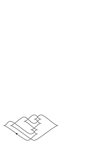
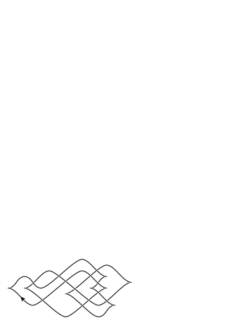
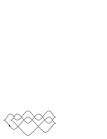
$7_{6}^{1+}$	$7_{6}^{2+}$	$7_{6}^{3+}$
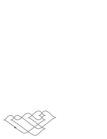
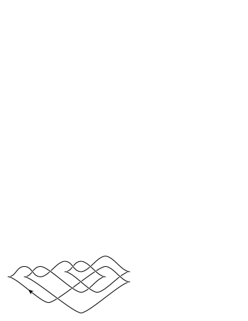
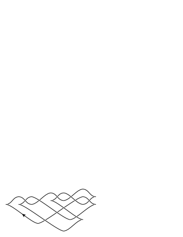
$r_{\medvert}(7_{6}^{1-})$	$r_{\medvert}(7_{6}^{2-})$	$r_{\medvert}(7_{6}^{3-})$

Figure 1. $\xi_{\pm}$-Legendrian classes of knots having topological type $7_{6}$

Proposition 1.

The following is a complete list, without repetitions, of $\xi_{+}$-Legendrian classes of topological type $7_{6}$ that have maximal possible Thurston–Bennequin number (which is $-8$):

(1) $$7_{6}^{1+}=-\mu(7_{6}^{1+}),\ -7_{6}^{1+}=\mu(7_{6}^{1+}),\ 7_{6}^{2+}=-\mu(7_{6}^{2+}),\ -7_{6}^{2+}=\mu(7_{6}^{2+}),\ 7_{6}^{3+},\ -7_{6}^{3+},\ \mu(7_{6}^{3+}),\ -\mu(7_{6}^{3+}).$$

Proof.

It established in [1] that:

1. the list (1) is complete;

2. $7_{6}^{1+}=-\mu(7_{6}^{1+})$, $7_{6}^{2+}=-\mu(7_{6}^{2+})$;

3. each of of $7_{6}^{1+}$, $7_{6}^{2+}$, and $7_{6}^{3+}$ has rotation number $1$, hence

   $$\bigl{\{}7_{6}^{1+},7_{6}^{2+},7_{6}^{3+},-\mu(7_{6}^{3+})\bigr{\}}\cap\bigl{\{}-7_{6}^{1+},-7_{6}^{2+},-7_{6}^{3+},\mu(7_{6}^{3+})\bigr{\}}=\varnothing;$$

It is conjectured but remained unsettled in [1] that the classes $7_{6}^{1+}$, $7_{6}^{2+}$, $7_{6}^{3+}$, and $-\mu(7_{6}^{3+})$ are pairwise distinct. To prove this, it suffices to establish the following two facts:

1. $7_{6}^{1+}\neq 7_{6}^{2+}$ and

2. $7_{6}^{3+}\neq-\mu(7_{6}^{3+})$.

In the proof, we use the diagrams $R_{1}$–$R_{8}$ shown in Figure 2.

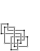
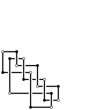
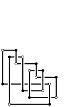
$R_{1}$		$R_{2}$		$R_{3}$		$R_{4}$
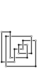
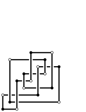
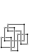
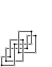
$R_{5}$		$R_{6}$		$R_{7}$		$R_{8}$

Figure 2. Rectangular diagrams representing the knot $7_{6}$ (or its mirror image). Black vertices are positive, and white ones are negative

To prove each of the statements (d) and (e) we follow the lines of the proof of [5, Proposition 2.3]. Similarly to the $6_{2}$ case, the orientation-preserving symmetry group of the knot $7_{6}$ is $\mathbb{Z}_{2}$ (see [7, 9]), we denote by $\sigma$ a self-homeomorphism of $\mathbb{S}^{3}$ representing the only non-trivial element of this group. The automorphism of the fundamental group of $\mathbb{S}^{3}\setminus\widehat{R}_{1}$ induced by the restriction of $\sigma$ to $\mathbb{S}^{3}\setminus\widehat{R}_{1}$ is denoted by $\sigma_{*}$. (This automorphism is defined up to an internal one. We will make a concrete choice below.)

Like $6_{2}$, the knot $7_{6}$ is fibered and has genus two [10, 6].

Proof of (d). One can immediately see from Figures 1 and 2 that

(2) $$\mathscr{L}_{+}(R_{1})=7_{6}^{1+}\quad and\quad\mathscr{L}_{+}(R_{2})=7_{6}^{2+}.$$

It is a direct check that $\mathscr{E}\bigl{(}S_{\overrightarrow{\mathrm{II}}}(R_{1})\bigr{)}=\mathscr{E}\bigl{(}S_{\overrightarrow{\mathrm{II}}}(R_{6})\bigr{)}$ and $\mathscr{E}\bigl{(}S_{\overleftarrow{\mathrm{I}}}(R_{2})\bigr{)}=\mathscr{E}\bigl{(}S_{\overleftarrow{\mathrm{I}}}(R_{6})\bigr{)}$, which implies

(3) $$\mathscr{L}_{+}(R_{6})=7_{6}^{2+},\quad\mathscr{L}_{-}(R_{6})=\mathscr{L}_{-}(R_{1})$$

(the class $\mathscr{L}_{-}(R_{1})$ coincides with $7_{6}^{3-}$, which does not play a role here).

One also finds that

$$\mathop{tb}\nolimits_{+}(R_{1})=\mathop{tb}\nolimits_{+}(R_{2})=\mathop{tb}\nolimits_{+}(R_{6})=-8,\quad\mathop{tb}\nolimits_{-}(R_{1})=\mathop{tb}\nolimits_{-}(R_{2})=\mathop{tb}\nolimits_{-}(R_{6})=-1,$$

hence, any Seifert surface for the knot $7_{6}$ is $+$-compatible and $-$-compatible with any of $R_{1}$, $R_{2}$, and $R_{6}$ (see [5, Definition 2.6]).

Now we choose a Seifert surface for $\widehat{R}_{1}$. Our choice is shown, in the rectangular form, in Figure 3 together with the torus projections of the chosen generators of the fundamental group of the surface.

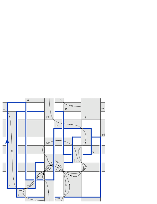
Figure 3. Rectangular diagram $\Pi_{1}$ with $\partial\Pi_{1}=R_{1}$

It is a direct check that $\widehat{\Pi}_{1}$ is orientable and has genus two. One can also see that the homotopy class of $\partial\widehat{\Pi}_{1}=\widehat{R}_{1}$ in $\widehat{\Pi}_{1}$ is presented by the element

(4) $$x_{1}x_{2}x_{3}x_{4}x_{1}^{-1}x_{2}^{-1}x_{3}^{-1}x_{4}^{-1}.$$

The generators $x_{i}$ are chosen so as to have

(5) $$\sigma_{*}(x_{i})=x_{i}^{-1},\quad i=1,2,3,4,$$

which will be seen in a moment. They are also shown in Figure 4 with

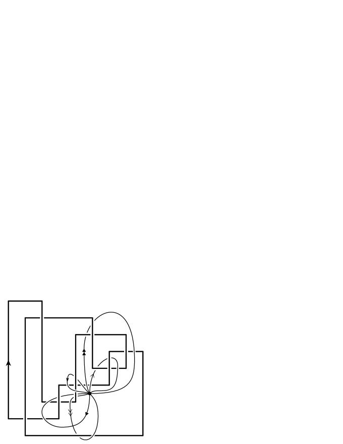
Figure 4. The generators $x_{1}$, $x_{2}$, $x_{3}$, $x_{4}$, and $u$ of $\pi_{1}(\mathbb{S}^{3}\setminus\widehat{R}_{1})$

an additional generator $u$ such that

(6) $$\sigma_{*}(u)=x_{2}^{-1}u.$$

One can verify, using the Wirtinger presentation of $\pi_{1}(\mathbb{S}^{3}\setminus\widehat{R}_{1})$, that $x_{1}$, $x_{2}$, $x_{3}$, $x_{4}$, and $u$ generate the fundamental group of $\widehat{R}_{1}$, and the following list can be taken for a set of defining relations:

$$ux_{1}u^{-1}=x_{4}^{2}x_{2}^{-1},\quad ux_{2}u^{-1}=x_{2}x_{4}^{-1}x_{2}x_{3}x_{2}x_{4}^{-1},\quad ux_{3}u^{-1}=x_{4}x_{2}^{-1},\quad ux_{4}u^{-1}=x_{4}x_{1}^{-1}x_{4}x_{2}^{-1}.$$

These relations are clearly preserved by the substitution $x_{i}\mapsto x_{i}^{-1}$ ($i=1,2,3,4$), $u\mapsto x_{2}^{-1}u$, which, therefore, defines an automorphism of $\pi_{1}(\mathbb{S}^{3}\setminus\widehat{R}_{1})$. This automorphism is an involution that preserves the conjugacy class of the element (4) and the homology class $[u]\in H_{1}(\mathbb{S}^{3}\setminus\widehat{R}_{1};\mathbb{Z})$. This implies that this automorphism is induced by a self-homeomorphism of $\mathbb{S}^{3}\setminus\widehat{R}_{1}$ taking $\widehat{\Pi}_{1}\setminus\widehat{R}_{1}$ to itself and preserving the orientations of $\mathbb{S}^{3}$ and $\widehat{\Pi}_{1}$. Such a homeomorphism must be isotopic to $\sigma$ (restricted to $\mathbb{S}^{3}\setminus\widehat{R}_{1}$), which verifies (5) and (6).

This means, that $\sigma$ can be chosen so as to have $\sigma(\widehat{\Pi}_{1})=\widehat{\Pi}_{1}$ and $\sigma^{2}=\mathrm{id}$. We may also assume that, for each $i=1,2,3,4$, the homeomorphism $\sigma$ takes a loop representing $x_{i}$ to the inverse of itself. We cut $\widehat{\Pi}_{1}$ along these loops to get an octagon with a hole. Shown in Figure 5 on the left

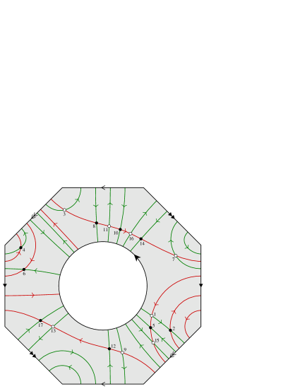
Figure 5. Dividing configurations $(\delta_{1}^{+},\delta_{1}^{-})$ and $(\delta_{1}^{+},\sigma(\delta_{1}^{-}))$

is a canonic dividing configuration, which we denote by $(\delta_{1}^{+},\delta_{1}^{-})$, on the cut surface, with $\delta_{1}^{+}$ shown in green and $\delta_{1}^{-}$ in red. The right picture in Figure 5 shows the dividing configuration $(\delta_{1}^{+},\sigma(\delta_{1}^{-}))$ (for a specific choice of $\sigma$). One can see that both dividing configurations have the same dividing code, which is

(7) $$\{(1,2,3,4),(5),(6,7,8),(9,10),(11,12),(13,14),(15),(16,17)\},\\ \{(1,5,15,6,1),(2),(3,8,11,10,16,14,7,4,9,12,13,17,3)\}.$$

The set $\{\delta_{1}^{-},\sigma(\delta_{1}^{-})\}$ is $-$-representative for $R_{1}$, and hence, for $R_{6}$ (see [5, Definition 2.8]). In view of (2) and (3), by [5, Theorem 2.1 and Corollary 2.1] the equality $7_{6}^{1+}=7_{6}^{2+}$ would imply the existence of a proper realization $(\Pi,\phi)$ of $(\delta_{1}^{+},\delta_{1}^{-})$ or $(\delta_{1}^{+},\sigma(\delta_{1}^{-}))$ such that $\partial\Pi$ is exchange-equivalent to $R_{6}$. Since $(\delta_{1}^{+},\delta_{1}^{-})$ and $(\delta_{1}^{+},\sigma(\delta_{1}^{-}))$ are isomorphic, they have the same sets of realizations (if not requested to be proper).

An exhaustive search (using the script [2]) results in exactly four, up to combinatorial equivalence, realizations $(\Pi,\phi)$ of $(\delta_{1}^{+},\delta_{1}^{-})$ such that $\partial\Pi$ is a rectangular diagram representing a knot of topological type $7_{6}$. These are shown in Figure 6.

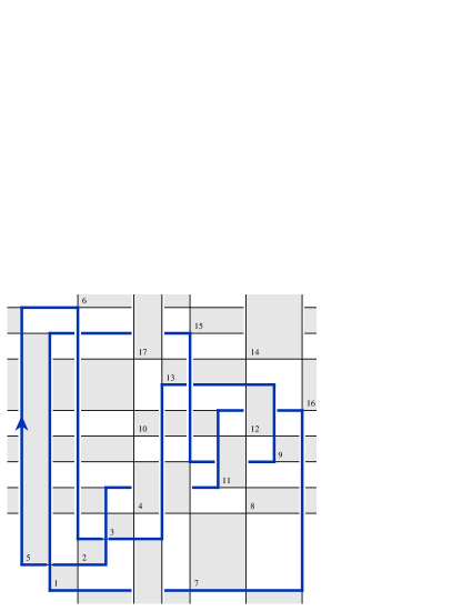
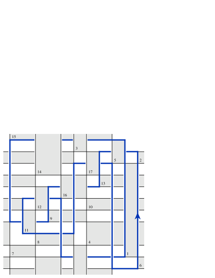
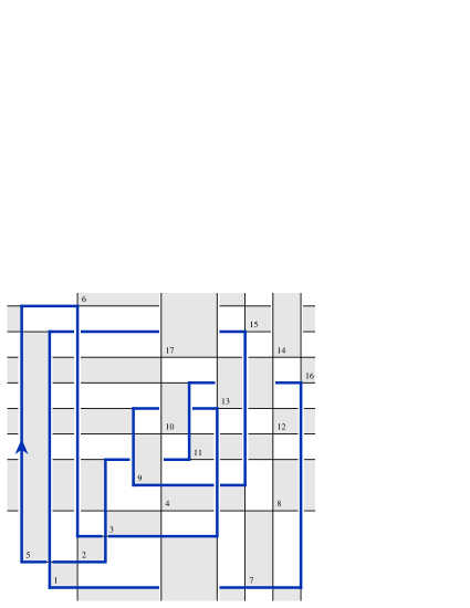
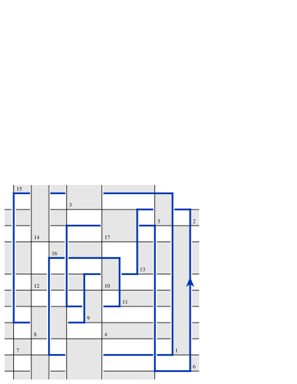
Figure 6. All realizations $\Pi$ of $(\delta_{1}^{+},\delta_{1}^{-})$ with $\partial\Pi$ representing the knot $7_{6}$

The boundaries of the obtained rectangular diagrams of a surface are $R_{1}$, $-\mu(R_{1})$, $R_{5}$, and $-\mu(R_{5})$. None of these rectangular diagrams of a knot admits a non-trivial exchange move, and none of them is combinatorially equivalent to $R_{6}$. Thus, $R_{6}\notin\mathscr{E}(R_{1})\cup\mathscr{E}(R_{5})\cup\mathscr{E}(-\mu(R_{1}))\cup\mathscr{E}(-\mu(R_{5}))$. Therefore, $7_{6}^{1+}\neq 7_{6}^{2+}$.

Remark 1.

At a very premature stage of the work presented in [4, 5] we expected that whenever rectangular diagrams of a knot $R$, $R^{\prime}$ are such that $\mathscr{L}_{+}(R)=\mathscr{L}_{+}(R^{\prime})$ and $\mathscr{L}_{-}(R)=\mathscr{L}_{-}(R^{\prime})$, and $\Pi$ is a rectangular diagram of a surface $\Pi$ with $\partial\Pi=R$ we must have another rectangular diagram of a surface $\Pi^{\prime}$ with $\partial\Pi^{\prime}=R^{\prime}$ having the same dividing code as $\Pi$ has. To test this expectation, for which we did not have enough grounds, we picked the first rectangular diagram $R$ from [1] for which the data of [1] implied $\mathscr{L}_{\pm}(R)=\mathscr{L}_{\pm}(-\mu(R))$ and $R\neq-\mu(R)$, and this diagram was the $R_{1}$ in Figure 2 above. We also constructed a rectangular diagram representing a Seifert surface for $\widehat{R}_{1}$, which was the $\Pi_{1}$ shown in Figure 4. Then, after searching all realizations of the dividing code of $\Pi_{1}$ we were delighted to see among them a diagram $\Pi^{\prime}$ with $\partial\Pi^{\prime}=-\mu(R)$ (which is the top right in Figure 6). This encouraged us to continue this work.

However, as we realized later, the existence of such $\Pi^{\prime}$ did not follow from our hypotheses, and the confirmation of our expectation by this example was accidental and occurred mainly to the fact that the dividing configurations $(\delta_{1}^{+},\delta_{1}^{-})$ and $(\delta_{1}^{+},\sigma(\delta_{1}^{-}))$ were isomorphic (another lucky circumstance was that the diagram $R$, and hence $-\mu(R)$, did not admit any non-trivial exchange move). The point is that $\Pi^{\prime}$ is a proper realization of $(\delta_{1}^{+},\sigma(\delta_{1}^{-}))$, but not of $(\delta_{1}^{+},\delta_{1}^{-})$, whereas our method does not say anything about the use of non-proper realizations (they may be discarded).

Proof of (e). We follow exactly the same steps as in the proof of the part (d), so we omit the details except for those that are different in this case. We now use the Seifert surface for $\widehat{R}_{7}$ presented by rectangular diagram $\Pi_{2}$ shown in Figure 7 together with new generators $y_{1},y_{2},y_{3},y_{4}$ of

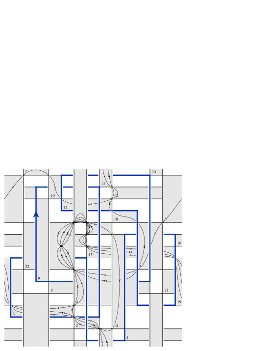
Figure 7. Rectangular diagram $\Pi_{2}$ with $\partial\Pi_{2}=R_{7}$

the fundamental group of $\widehat{\Pi}_{2}$. A complete set of generators of $\pi_{1}(\mathbb{S}^{3}\setminus\widehat{R}_{7})$ is shown in Figure 8,

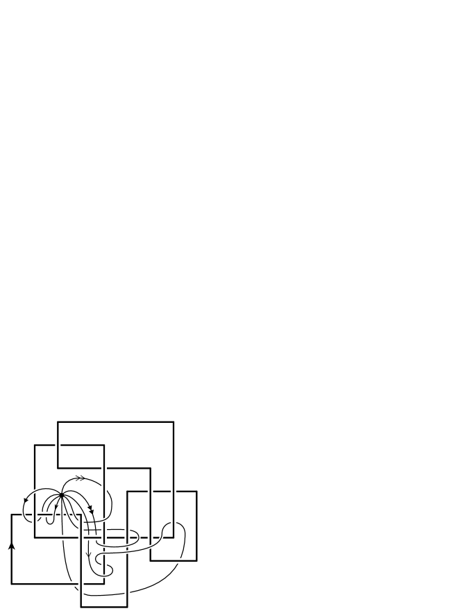
Figure 8. The generators $y_{1}$, $y_{2}$, $y_{3}$, $y_{4}$, and $v$ of $\pi_{1}(\mathbb{S}^{3}\setminus\widehat{R}_{7})$

which can be used to verify the following defining relations:

$$v^{-1}y_{1}v=y_{1}y_{4}^{-1}y_{1}y_{3},\quad v^{-1}y_{2}v=y_{3}^{-1}y_{2}y_{3}y_{1}y_{3}y_{2},\quad v^{-1}y_{3}v=y_{2}y_{3},\quad v^{-1}y_{4}v=y_{3}^{-1}y_{2}^{-2}.$$

One can see from this that, for a smart choice of the involution $\sigma$, we will have

$$\sigma_{*}(v)=vy_{3}^{-1},\quad\sigma_{*}(y_{i})=y_{i}^{-1},\quad i=1,2,3,4.$$

We denote by $(\delta_{2}^{+},\delta_{2}^{-})$ a canonic dividing configuration of $\widehat{\Pi}_{2}$. After cutting the surface along the loops $y_{i}$, $i=1,2,3,4$, this configuration looks as shown in Figure 9 on the left.

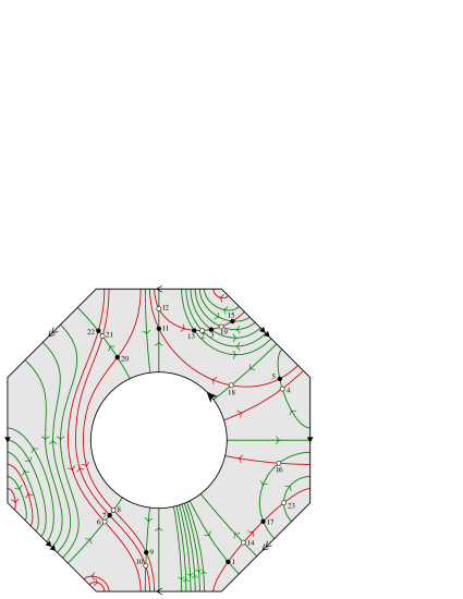
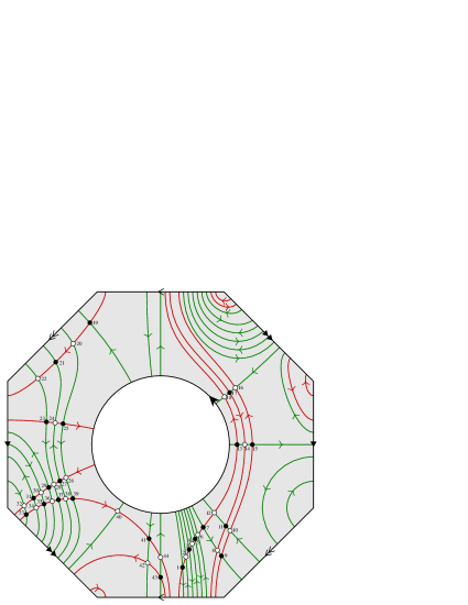
Figure 9. Dividing configurations $(\delta_{2}^{+},\delta_{2}^{-})$ and $(\delta_{2}^{+},\sigma(\delta_{2}^{-}))$

The right picture in Figure 9 shows the dividing configuration $(\delta_{2}^{+},\sigma(\delta_{2}^{-}))$ (for a concrete choice of $\sigma$). The dividing configurations $(\delta_{2}^{+},\delta_{2}^{-})$ and $(\delta_{2}^{+},\sigma(\delta_{2}^{-}))$ have the following dividing codes, respectively:

(8) $$\{(1,2),(3,4,5,6,7,8),(9,10),(11,12),(13,14),(15,16,17,18),(19),(20,21,22,23)\},\\ \{(4,22,6,20,8,9,12,13,2,3,19,15,16),(5,18,11,10,7,21,5),(14,17,23,1,14)\}$$

and

(9) $$\{(19,32,33,6),(7,8,9,22,23,28,37,2),(3,36,29,40),(41,42),(43,44),\\ (1,38,27,24,21,10,11,12),(13,14,15,30,35,4),(5,34,31,20,25,26,39,16,17,18)\},\\ \{(19,20,21,22,19),(33,34,35,36,37,38,39,40,41,44,17,14,11,8,33),\\ (26,27,28,29,30,31,32,9,10,15,16,1,2,3,4,5,6,7,12,13,18,43,42,23,24,25)\}.$$

The dividing code (8) has exactly three realizations $(\Pi,\phi)$ with $\widehat{\partial\Pi}$ isotopic to $7_{6}$. For all of them we have $\partial\Pi\in\mathscr{E}(R_{7})$.

The dividing code (9) has exactly $12$ realizations $(\Pi,\phi)$ with $\widehat{\partial\Pi}$ isotopic to $7_{6}$ (the script [2] produces 20 realizations for this dividing code, but in 8 cases the boundary $\partial\Pi$ represents the connected sum $3_{1}\#4_{1}$). One of these is shown in Figure 10.

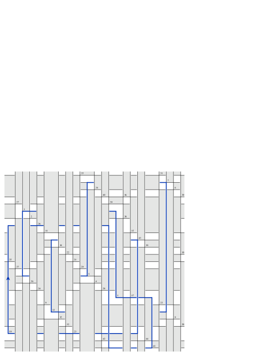
Figure 10. A realization of $(\delta_{2}^{+},\sigma(\delta_{2}^{-}))$

In all $12$ cases we again have $\partial\Pi\in\mathscr{E}(R_{7})$.

Thus, we need not bother to check which of the realizations are proper as it follows from what was just said and the results of [5] that

(10) $$\text{the conditions }\mathscr{L}_{+}(R)=\mathscr{L}_{+}(R_{7})\text{ and }\mathscr{L}_{-}(R)=\mathscr{L}_{-}(R_{7})\text{ holding simultaneously imply }R\in\mathscr{E}(R_{7}).$$

It is a direct check that

$$\mathscr{L}_{+}(R_{3})=7_{6}^{3+},\quad\mathscr{E}\bigl{(}S_{\overrightarrow{\mathrm{I}}}(\mu(R_{3}))\bigr{)}=\mathscr{E}\bigl{(}S_{\overrightarrow{\mathrm{I}}}(R_{7})\bigr{)},\quad\text{and}\quad\mathscr{E}\bigl{(}S_{\overleftarrow{\mathrm{II}}}(R_{7})\bigr{)}=\mathscr{E}\bigl{(}S_{\overleftarrow{\mathrm{II}}}(-\mu(R_{7}))\bigr{)}.$$

This implies

$$\mathscr{L}_{+}(R_{7})=\mu(7_{6}^{3+})\quad\text{and}\quad\mathscr{L}_{-}(R_{7})=\mathscr{L}_{-}(-\mu(R_{7})).$$

On the other hand, we have $\mathscr{E}(R_{7})\neq\mathscr{E}(-\mu(R_{7}))$. Therefore,

$$\mu(7_{6}^{3+})=\mathscr{L}_{+}(R_{7})\neq\mathscr{L}_{+}(-\mu(R_{7}))=-7_{6}^{3+},$$

which implies (e). ∎

Proposition 2.

The following is a complete list, without repetitions, of $\xi_{-}$-Legendrian classes of topological type $7_{6}$ that have maximal possible Thurston–Bennequin number (which is $-1$):

(11) $$7_{6}^{1-}=\mu(7_{6}^{1-})=-7_{6}^{1-}=-\mu(7_{6}^{1-}),\ 7_{6}^{2-}=-\mu(7_{6}^{2-}),\ -7_{6}^{2-}=\mu(7_{6}^{2-}),\ 7_{6}^{3-}=-\mu(7_{6}^{3-}),\ -7_{6}^{3-}=\mu(7_{6}^{3-}).$$

Proof.

It is established in [1] that the list is complete and the classes are pairwise distinct except for $7_{6}^{2-}$ and $\mu(7_{6}^{2-})=-7_{6}^{2-}$, which may be coincident. So, we only need to show that $7_{6}^{2-}\neq\mu(7_{6}^{2-})$.

By a direct check we find: $\mathscr{L}_{-}(r_{\medvert}(R_{4}))=7_{6}^{2-}$,

$$\mathscr{E}\bigl{(}S_{\overleftarrow{\mathrm{I}}}(R_{7})\bigr{)}=\mathscr{E}\bigl{(}S_{\overleftarrow{\mathrm{I}}}(R_{8})\bigr{)},\quad\mathscr{E}\bigl{(}S_{\overleftarrow{\mathrm{II}}}(R_{7})\bigr{)}=\mathscr{E}\bigl{(}S_{\overrightarrow{\mathrm{II}}}(r_{\medvert}(R_{4}))\bigr{)},\quad\mathscr{E}\bigl{(}S_{\overrightarrow{\mathrm{II}}}(R_{8})\bigr{)}=\mathscr{E}\bigl{(}S_{\overrightarrow{\mathrm{II}}}(\mu(r_{\medvert}(R_{4})))\bigr{)},$$

which imply

$$\mathscr{L}_{+}(R_{7})=\mathscr{L}_{+}(R_{8}),\quad\mathscr{L}_{-}(R_{7})=7_{6}^{2-},\quad\text{and}\quad\mathscr{L}_{-}(R_{8})=\mu(7_{6}^{2-}).$$

Since $\mathscr{E}(R_{7})\neq\mathscr{E}(R_{8})$, it follows from (10) that $7_{6}^{2-}\neq\mu(7_{6}^{2-})$. ∎

References

- [1] W. Chongchitmate, L. Ng. An atlas of Legendrian knots. Exp. Math. 22 (2013), no. 1, 26–37; arXiv:1010.3997.
- [2] I. Dynnikov. A Python code for searching all realizations of a dividing configuration. https://arxiv.org/src/1712.06366v2/anc
- [3] I. Dynnikov, M. Prasolov. Bypasses for rectangular diagrams. A proof of the Jones conjecture and related questions (Russian), Trudy MMO 74 (2013), no. 1, 115–173; translation in Trans. Moscow Math. Soc. 74 (2013), no. 2, 97–144; arXiv:1206.0898.
- [4] I. Dynnikov, M. Prasolov. Rectangular diagrams of surfaces: representability, Matem. Sb. 208 (2017), no. 6, 55–108; translation in Sb. Math. 208 (2017), no. 6, 781–841, arXiv:1606.03497.
- [5] I. Dynnikov, M. Prasolov. Rectangular diagrams of surfaces: distinguishing Legendrian knots. Preprint, arXiv:1712.06366.
- [6] K. Murasugi. On a certain subgroup of the group of an alternating link. Amer J. Math., 85 (1963), 544–550.
- [7] K. Kodama, M. Sakuma. Symmetry groups of prime knots up to 10 crossings. Knots 90 (Osaka, 1990), 323–340, de Gruyter, Berlin, 1992.
- [8] P.Ozsváth, Z.Szabó, D.Thurston. Legendrian knots, transverse knots and combinatorial Floer homology, Geometry and Topology, 12 (2008), 941–980, arXiv:math/0611841.
- [9] M. Sakuma. The geometries of spherical Montesinos links. Kobe J. Math. 7 (1990), no. 2, 167–190.
- [10] J. Stallings. On fibering certain -manifolds. Topology of -manifolds and related topics (Proc. The Univ. of Georgia Institute, 1961), pp. 95–100, Prentice-Hall, Englewood Cliffs, N.J.