Bosonic Fractional Quantum Hall States on a Finite Cylinder

Abstract

We investigate the ground state properties of a bosonic Harper-Hofstadter model with local interactions on a finite cylindrical lattice with filling fraction $\nu=1/2$. We find that our system supports topologically ordered states by calculating the topological entanglement entropy, and its value is in good agreement with the theoretical value for the $\nu=1/2$ Laughlin state. By exploring the behaviour of the density profiles, edge currents and single-particle correlation functions, we find that the ground state on the cylinder shows all signatures of a fractional quantum Hall state even for large values of the magnetic flux density. Furthermore, we determine the dependence of the correlation functions and edge currents on the interaction strength. We find that depending on the magnetic flux density, the transition towards Laughlin-like behaviour can be either smooth or happens abruptly for some critical interaction strength.

I Introduction

An exciting approach for gaining novel insights into the physics of strongly correlated many-body quantum systems is provided by the concept of quantum simulation Cirac and Zoller (2012); Johnson et al. (2014). A particularly promising platform for the simulation of many-body quantum lattice systems are ultracold atoms trapped in periodic electromagnetic fields Jaksch et al. (1998); Greiner et al. (2002); Bloch et al. (2008); Jördens et al. (2008); Gullans et al. (2012). In state-of-the-art optical lattice experiments one can control, manipulate and observe atoms with single-site resolution Bakr et al. (2009, 2010); Sherson et al. (2010); C. Weitenberg et al. (2011); Gericke et al. (2008); Würtz et al. (2009); Cheuk et al. (2015) which opens up unprecedented possibilities for the realization and observation of novel physical phenomena.

Quantum Hall systems are a fundamental paradigm in condensed matter physics v. Klitzing et al. (1980); Tsui et al. (1982a, b), and thus the experimental realization of these systems in optical lattices has attracted tremendous interest in recent years Jaksch and Zoller (2003); Aidelsburger et al. (2013); Miyake et al. (2013); Aidelsburger et al. (2014). Of particular interest are fractional quantum Hall states Cooper and Dalibard (2013); Tsui et al. (1982a); Cooper (2008); Harper et al. (2014); Scaffidi and Simon (2014) which require interactions between the particles Tai et al. (2017) and are thus difficult to realize.

Fractional quantum Hall systems on lattices are described by an extension of the Harper-Hofstadter (HH) model Hofstadter (1976) in order to account for interactions Harper (1955); Hofstadter (1976); Hafezi et al. (2007). The realization of fractional quantum Hall states requires appropriate filling fractions $\nu=n_{b}/n_{\phi}$ Tsui et al. (1982a); Laughlin (1983), where $n_{\phi}$ is the density of magnetic fluxes per plaquette and $n_{b}$ is the density of particles. In small lattice systems permitting exact diagonalisation (ED) calculations Sørensen et al. (2005); Hafezi et al. (2007); Möller and Cooper (2009); Sterdyniak et al. (2012) the properties of the ground state can be simply analyzed by calculating the overlap with the corresponding Laughlin wave function.

Larger-scale systems become theoretically accessible with density matrix renormalization group (DMRG) techniques White (1992, 1993), but require alternative methods for characterising the ground state features. For example, the presence of a gapped, insulating bulk and gapless edge modes in a fractional quantum Hall state gives rise to a uniform density in the bulk and a density spike near the edges Ciftja et al. (2011); Rezayi and Haldane (1994), chiral edge currents Halperin (1982); gang Wen (1992) and algebraically decaying one-particle correlation functions near the edge He et al. (2017); Gerster et al. (2017). Furthermore, an unambiguous indication of topological order of the ground state is the topological entanglement entropy, which can be calculated for Laughlin states Kitaev and Preskill (2006); Fendley et al. (2007); Dong et al. (2008). These observables have been used to characterize fractional quantum Hall states on a torus, a square lattice Gerster et al. (2017); He et al. (2017); Račiūnas et al. (2018) and ladder geometries Budich et al. (2017); Strinati et al. (2017); Petrescu et al. (2017). Other microscopic models supporting Laughlin states have been considered Cincio and Vidal (2013); Nielsen et al. (2013); Bauer et al. (2014) and a number of methods to characterize topologically ordered ground states have been proposed such as modular matrices and momentum polarization Cincio and Vidal (2013); Tu et al. (2013); Zaletel et al. (2013).

Recently, a theoretical proposal for the realization of cylindrical lattices has been put forward Łacki et al. (2016). This geometry is particularly well suited for investigating manifestations of gapless edge modes due to the two system boundaries in one direction and periodic boundary conditions (PBC) in the other direction. Furthermore, it has been shown that the cylinder geometry can support fractional quantum Hall states for Fermions and small system sizes using ED techniques Łacki et al. (2016).

Here we investigate ground states of the interacting HH model for bosons on a cylinder geometry with DMRG methods. We focus on states with filling fraction $\nu=1/2$ and show that the cylinder geometry supports topologically ordered states. More specifically, we calculate the topological entanglement entropy for a system with magnetic flux density $n_{\phi}=1/6$ and find that its value is very close to that of a $\nu=1/2$ Laughlin state in the continuum.

Our DMRG approach allows us to study how the density profile, the edge currents and single-particle correlation functions scale with the length of the cylinder and the magnitude of the on-site interaction. These calculations are performed in the as yet little explored regime of large flux densities where lattice effects become important. We find that all observables of interest exhibit the characteristic features of the Laughlin state in the case of large system sizes and hard-core bosons.

Finally, we address the dependence of the correlation functions and edge currents on the on-site interaction strength $U$ and find that the Laughlin-like behaviour is adapted continuously with increasing $U$ for $n_{\phi}=1/3$. On the other hand, we show that a slightly smaller flux density $n_{\phi}=1/4$ can give rise to an abrupt increase in the importance of the edge currents relative to the bulk.

This paper is organized as follows. In Sec. II we describe the geometry of the system and introduce the theoretical model. Our results are presented in Sec. III. The topological entanglement entropy is discussed in Sec. III.1, and the density profiles, currents and correlation functions are covered in Sec. III.2. The dependence of the correlation functions and edge currents on the interaction strength is presented in Sec. III.3. Finally, a discussion and summary of our results is provided in Sec. IV.

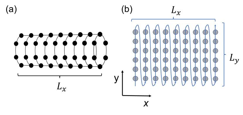
Figure 1: (Color online) (a) The system of interest is a cylindrical lattice with length $L_{x}$ and circumference $L_{y}$. (b) Rectangular lattice corresponding to the cylindrical lattice in (a). Threading through the two-dimensional lattice with $L_{x}\times L_{y}$ sites as indicated by the blue line allows one to map the system to a one-dimensional chain with long-range hopping terms.

II Model

We consider the interacting HH model for spinless bosons on a square lattice with $L_{x}$ sites in the $x$-direction and $L_{y}$ sites in the $y$-direction. We impose PBC along the $y$ direction, turning the lattice into a cylinder as shown in Fig. 1. The bosons are subject to a gauge field giving rise to a uniform magnetic field orthogonal to the lattice. The Hamiltonian of the system is

$$H=H_{\text{kin}}+H_{U}\,,$$ (1)

where $H_{\text{kin}}$ and $H_{U}$ describe the single-particle kinetic energy and the on-site interaction, respectively. We find

$$H_{\text{kin}}= -J\left[\sum_{x=1}^{L_{x}-1}\sum_{y=1}^{L_{y}}c^{\dagger}_{x,y}c_{x+1,y}\right.$$

$$\hskip 28.45274pt+\sum_{x=1}^{L_{x}}\sum_{y=1}^{L_{y}-1}e^{i2\pi x\phi}c^{\dagger}_{x,y}c_{x,y+1}$$

$$\hskip 28.45274pt\left.+\sum_{x=1}^{L_{x}}e^{i2\pi x\phi}c^{\dagger}_{x,L_{y}}c_{x,1}\right]+\text{H.c.}\,,$$ (2)

where $c_{x,y}$ is the annihilation operator for a boson at a site labelled by the coordinates $(x,y)$ and satisfying bosonic commutation relations $[c_{i},c_{j}^{\dagger}]=\delta_{ij}$ and $J$ is the hopping amplitude. Note that $H_{\text{kin}}$ in Eq. (2) is written in the Landau gauge. When a particle hops around a plaquette it picks up a phase $e^{i2\pi\phi}$, and hence the number of flux quanta per plaquette is $n_{\phi}\equiv\phi$.

The interaction term $H_{U}$ in Eq. (1) is defined as

$$H_{U}=U\sum_{x=1}^{L_{x}}\sum_{y=1}^{L_{y}}n_{x,y}(n_{x,y}-1)\,,$$ (3)

where $U$ is the on-site interaction strength and $n_{x,y}=c^{\dagger}_{x,y}c_{x,y}$ is the number operator at site $(x,y)$. We truncate the maximal occupation number of each site at $n_{\text{max}}$ in our numerical calculations. The required value of $n_{\text{max}}$ in order to achieve convergence depends on the interaction strength as specified in Sec. III. We also consider the hard-core boson limit $U/J\rightarrow\infty$ which can be realised by setting $n_{\text{max}}=1$.

We obtain the ground state of the system by performing DMRG calculations. To this end, we map the 2D lattice with PBC to a 1D lattice (Stoudenmire and White, 2012) as shown in Fig. 1(b). While the 2D model in Eq. (1) comprises only nearest-neighbour (NN) hopping terms, the mapping to 1D introduces hopping terms with range up to $L_{y}$. In order to efficiently treat these long-range hopping terms, we build the matrix product operator (MPO) that describes the 2D Hamiltonian with cylindrical boundary conditions using the finite automata technique Crosswhite and Bacon (2008). In this method, the MPOs are derived from a complex weighted finite automaton as described in Appendix A. All our DMRG calculations are carried out with the TNT library Al-Assam et al. (2017) and use $U(1)$ number conservation symmetry.

III Results

Here we present our DMRG results for the ground state on a cylinder with filling fraction $\nu=1/2$ and different values of $\phi$. We begin with a discussion of the topological entanglement entropy for a system with $\phi=1/6$ in Sec. III.1. Our calculations for the particle density, currents and correlation functions are presented in Sec. III.2 for $\phi=1/3$. All calculations in Secs. III.1 and III.2 correspond to the hard-core boson limit. This condition is relaxed in Sec. III.3, where we consider variable interaction strengths $U/J$. In particular, we present calculations of the bulk and edge currents for variable interaction strengths and two different magnetic flux densities.

III.1 Topological Entanglement Entropy

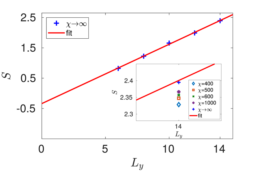
Figure 2: (Color online) Entanglement entropy $S$ for a cylinder of length $L_{x}=6$, filling fraction $\nu=1/2$ and $\phi=1/6$ as a function of circumference $L_{y}$. The blue crosses are the results of an extrapolation of $S$ to $\chi\rightarrow\infty$, and the red solid line is the linear fit to these values. The inset shows the data points obtained for different bond dimensions $\chi$ at $L_{y}=14$.

The topological order of quantum many-body states can be quantified using the topological entanglement entropy $\gamma$ as shown in Kitaev and Preskill (2006). A non-zero value of $\gamma>0$ unambiguously indicates topological order of the ground state and the presence of anyonic quasi-particle excitations. The topological entanglement entropy can be calculated from a correction to the area law Vidal et al. (2003); Eisert et al. (2010) for the entanglement entropy

$$S(L)=cL-\gamma\,,$$ (4)

where $L$ is the length of the system boundary created by dividing the system into two parts, and $c$ is a non-universal constant. DMRG calculations lend themselves particularly well for computing $\gamma$ since $S$ can be evaluated from the Schmidt values $\lambda_{i}$ entering the matrix product representation of the ground state,

$$S=-\text{tr}[\rho_{L}\ln(\rho_{L})]=-\sum_{i}|\lambda_{i}|^{2}\ln(|\lambda_{i}|^{2})\,,$$ (5)

where $\rho_{L}$ is the density matrix of the left part of the system after a cut.

We compute $S$ for the ground state in the cylinder geometry with filling fraction $\nu=1/2$ and $\phi=1/6$ for a cylinder of length $L_{x}=6$ and different values of the circumference $L_{y}$ as shown in Fig. 2. We perform the cut by dividing the cylinder in two equal parts, each consisting of $3\times L_{y}$ sites. Our DMRG calculations lead to a two-fold degenerate ground state for the considered system sizes due to the centre-of-mass degeneracies in the corresponding system on a torus Kol and Read (1993). In using Eq. (4) for calculating the topological entanglement entropy we thus assume that DMRG automatically selects the minimally entangled states Jiang et al. (2012), and that only Abelian anyons are present in the system Zhang et al. (2012).

We calculate $\gamma$ by extrapolating all data points for $S$ to $\chi\rightarrow\infty$ resulting in $S_{\infty}(L_{y})$. We then perform a linear fit to the values $S_{\infty}(L_{y})$ and obtain

$$\gamma\approx 0.34\pm 0.05\,,$$ (6)

where the error represents the 68% confidence interval of the linear fit to the $S_{\infty}$ values. This clearly demonstrates that the cylinder geometry supports topologically ordered ground states. Moreover, the value of $\gamma$ is in good agreement with the expected value of $\gamma=\ln\sqrt{2}\approx 0.347$ for a Laughlin state with filling fraction $\nu=1/2$ Fendley et al. (2007); Dong et al. (2008).

III.2 Particle density, edge currents and correlation functions

Here we present results for the particle density, the edge currents and the correlation functions of our system. More specifically, we consider the ground state of our cylindrical lattice in the hard-core boson limit and focus on the state with filling fraction $\nu=1/2$ and $\phi=1/3$.

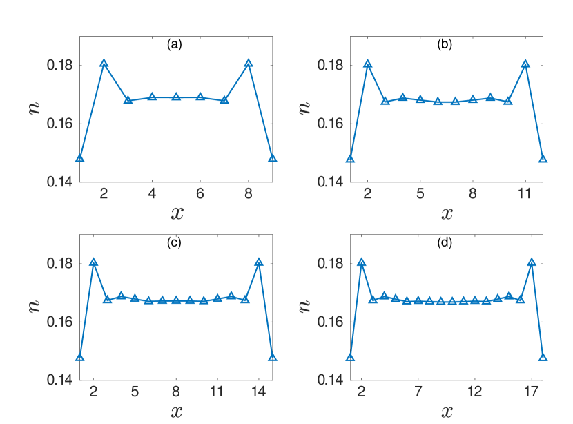
Figure 3: (Color online) Particle density $n$ as a function of the $x$ coordinate for system sizes $L_{x}\times L_{y}$: (a) $9\times 6$, (b) $12\times 6$, (c) $15\times 6$ and (d) $18\times 6$. $n$ is dimensionless. Lines connecting the data points are a guide to the eye, and all calculations have been performed with bond dimension $\chi=1000$.

Throughout this section, we consider a cylinder with circumference $L_{y}=6$ and four different values of $L_{x}$. These values are chosen such that the ground state is non-degenerate in order to obtain unambiguous results for the observables of interest. System sizes leading to non-degenerate ground states can be found by first considering a torus where unique ground states can be obtained for specific values of $L_{x}$ and $L_{y}$ Kol and Read (1993). For all cases investigated here the corresponding cylinder geometry also features a non-degenerate ground state.

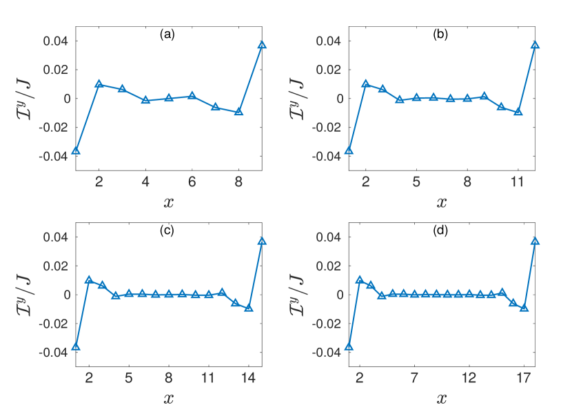
Figure 4: (Color online) Current around the cylinder $\mathcal{I}^{y}$ as a function of the $x$ coordinate for system sizes $L_{x}\times L_{y}$: (a) $9\times 6$, (b) $12\times 6$, (c) $15\times 6$ and (d) $18\times 6$. Lines connecting the data points are a guide to the eye, and all calculations are for bond dimension $\chi=1000$.

We start by examining the local density defined as

$$n(x)=\frac{1}{L_{y}}\sum\limits_{y=1}^{L_{y}}\langle c^{\dagger}_{x,y}c_{x,y}\rangle\,,$$ (7)

where we take the average over the circumference because of the rotational symmetry of the cylinder. The density profile of the ground state is shown in Fig. 3 for four different lengths of the cylinder. In all cases, the density of the central ring is $n\approx 0.17\approx n_{b}$ ($n_{b}$: mean number of bosons), and the density profile exhibits a pronounced spike at the second ring. As the length of the cylinder increases, the density profile increasingly resembles the density profile of the corresponding Laughlin state in the continuum Ciftja et al. (2011); Rezayi and Haldane (1994).

Next, we investigate the mean currents $\mathcal{I}^{y}$ flowing around the cylinder in $y$-direction,

$$\mathcal{I}^{y}(x)=\frac{1}{L_{y}}\sum\limits_{y=1}^{L_{y}}\langle iJe^{i2\pi x\phi}c_{x,y}^{\dagger}c_{x,y+1}+\text{H.c.}\rangle\,,$$ (8)

where the average is taken over the circumference of the cylinder and site $L_{y}+1$ corresponds to site $1$ due to the rotational symmetry of the cylinder. The currents for different $x$ coordinates and variable cylinder lengths are shown in Fig. 4. We find that the current is dominant at the edges and takes on its smallest values near the center of the cylinder where the currents fluctuate around zero. As the length of the cylinder increases, the current fluctuations in the bulk become smaller. Note that the currents flow in opposite directions at the two edges of the cylinder, which signifies their chiral nature. Our results for the currents are consistent with gapless edge states and an insulating bulk and are qualitatively similar to those for a $\nu=1/2$ Laughlin state.

Finally we consider the (normalized) one-particle correlation functions along the $y$-direction,

$$C^{y}(x,\Delta y)=\frac{\langle c_{x,1}^{\dagger}c_{x,1+\Delta y}\rangle}{n(x)}.$$ (9)

The correlation function $C^{y}(x,\Delta y)$ on ring $x$ is a measure for correlations between two sites that are $\Delta y$ apart in the radial direction. The correlation functions for a cylinder of length $L_{x}=18$ and circumference $L_{y}=6$ are shown in Fig. 5. We find that the correlation function on the first ring ($x=1$) stands out from all others since it decays significantly slower with $\Delta y$ than all other correlation functions. Note that a qualitatively similar behaviour of the correlation functions is found for all other system sizes investigated in Figs. 3 and 4. Our results are consistent with an algebraic decay of correlation functions at the edge and an exponential decay in the bulk, as expected for a fractional quantum Hall state with gapless edge modes and gapped bulk excitations.

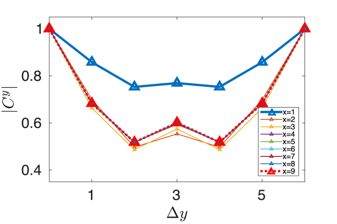
Figure 5: (Color online) (a) Correlation functions $C^{y}$ for system size $L_{x}\times L_{y}$: $18\times 6$. Each line represents the correlation function around a ring identified by its $x$-coordinate. Only the rings from $x=1$ to $x=L_{x}/2$ are shown due to the inversion symmetry of the cylinder. Lines connecting the data points represent a guide to the eye and all calculations are for bond dimension $\chi=1000$.

III.3 Interaction-strength dependence

All results in Sec. III.2 were obtained for hard-core bosons, i.e., infinitely strong on-site interactions. Since interactions in the condensed matter systems of interest are not infinitely strong, the question arises how finite interaction strengths modify these results. Here we address this question and calculate the correlation functions and currents for a cylindrical lattice of length $L_{x}=9$ and circumference $L_{y}=6$, $\phi=1/3$ and $\nu=1/2$ for variable interaction strengths $U/J$.

We begin with a discussion of the correlation functions $C^{y}(x,\Delta y)$ defined in Eq. (9). In the non-interacting case $U=0$ we can find an analytical solution of the ground state which is presented in Appendix B. This exact solution implies that all correlation functions are constant, see Fig. 6(a). Our numerical results for $C^{y}(x,\Delta y)$ with $x=1$ and for the central ring ($x=5$) are shown in Figs. 6(b-d) for $U>0$. For small values of $U/J$, the correlations at the edge decay faster than those in the bulk [see Figs. 6(b) and (c)]. Note that this is in stark contrast to the hard-core boson case where the correlation function at the edge decays slower than all other correlation functions, see Sec. III.2. We find that the decay of correlations at the edge becomes slower than that of the bulk correlations for $U/J\gtrsim 2.5$, and for $U/J=8$ the correlation functions are practically indistinguishable from their hard-core boson counterparts as shown in Fig. 6(d). These results are consistent with ED calculations for smaller systems, showing that for $\phi>0.2$ the interaction strength must exceed $U/J\gtrsim\phi$ in order to induce Laughlin-like states.

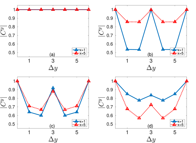
Figure 6: (Color online) Correlation functions $C^{y}$ for an $L_{x}\times L_{y}=9\times 6$ lattice, with $\nu=1/2$ and $\phi=1/3$. The interaction strength takes on values (a) $U/J=0$, (b) $U/J=0.1$, (c) $U/J=2$, (d) $U/J=8$. Lines connecting the data points are a guide to the eye. The maximal occupation number at each site is $n_{\text{max}}=4$ and the bond dimension is $\chi=500$. For $U=0$ we used $n_{\text{max}}=9$, which is equal to the total number of particles in the system.

In order to systematically investigate how the hard-core boson limit is approached with increasing interaction strength, we focus on the currents defined in Eq. (8) and introduce the quantity

$$R_{\mathcal{I}}=\frac{|\mathcal{I}^{y}(1)|}{\sigma(\text{bulk})}\,,$$ (10)

where $\mathcal{I}^{y}(1)$ is the edge current and $\sigma(\text{bulk})$ is the standard deviation of the currents in the bulk. The ratio $R_{J}$ quantifies the relative importance of the edge current with respect to the currents in the bulk. Our results for $R_{J}$ as a function of $U/J$ are shown in Fig. 7. We find that the bulk currents dominate the edge currents for $U/J<0.5$, and the ratio $R_{\mathcal{I}}$ increases monotonically with $U/J$ until it starts saturating near $U/J\approx 5$. Similarly to the correlation functions, we thus find that Laughlin-like behaviour of the currents requires interaction strengths exceeding $U/J\gtrsim\phi$.

A striking feature of Fig. 7(a) is that the transition from zero to strong interactions is completely smooth and does not feature a sharp phase transition. Since a fractional quantum Hall state requires interactions, a sharp transition between a state with no topological order for $U=0$ and a topologically ordered state for $U>0$ is expected in the continuum. This is confirmed by ED calculations for small systems Hafezi et al. (2007) indicating that this topological phase transition happens at $U=0$ for small values of $\phi<0.2$. The reason for our observation of a smooth transition is that we consider a large value of $\phi=1/3$ where there is a significant difference between the continuum and the lattice. The overlap between the Laughlin state on the lattice and the actual ground state is small for $U=0$ and increases gradually with increasing $U/J$ Hafezi et al. (2007). This gradual increase of the overlap is consistent with our results for $R_{\mathcal{I}}$ in Fig. 7(a).

A different situation should arise for smaller values of $\phi$ where the overlap with the Laughlin state at $U=0$ is larger Hafezi et al. (2007). In order to investigate this we consider a system with a smaller magnetic flux density $\phi=1/4$. Our results for $R_{\mathcal{I}}$ are shown in Fig. 7(b), showing that $R_{\mathcal{I}}$ increases sharply with $U/J$ until $U/J\approx 3$, where it levels off and subsequently decreases slightly. Most importantly, $R_{\mathcal{I}}$ exhibits a sharp jump at $U/J\approx 9.8$. The corresponding currents before and after the jump are shown in Figs. 7(c) and (d), respectively. For $U/J=9.6$ the current grows approximately linearly with the position $x$ of the ring along the cylinder axis. On the contrary, for $U/J=9.9$ the dependence of the current on $x$ is similar to that of the hard-core boson case for $\phi=1/3$, see Fig. 6(d).

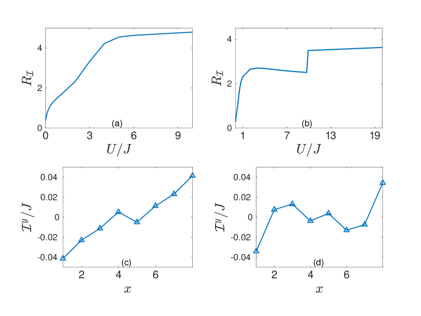
Figure 7: (Color online) (a) $R_{\mathcal{I}}$ as defined in Eq. (10) for a system of size $L_{x}\times L_{y}=9\times 6$, $\phi=1/3$ and $\nu=1/2$. (b) $R_{\mathcal{I}}$ for a system of size $L_{x}\times L_{y}=8\times 4$, $\phi=1/4$ and $\nu=1/2$. For the DMRG calculations, we used a maximum occupation number per site $n_{\text{max}}=4$, and bond dimension up to $\chi=300$. The current $\mathcal{I}^{y}(x)$ for the system in (b) is shown in (c) and (d) for $U/J=9.6$ and $U/J=9.9$, respectively. Lines connecting the data points in (c) and (d) are a guide to the eye.

IV Discussion and Summary

In this work, we have presented DMRG calculations for ground states of an interacting bosonic Harper-Hofstadter model on a cylinder geometry. In order to apply DMRG methods to this system, we mapped the two-dimensional grid to a one-dimensional chain with long-range hopping terms and constructed the corresponding matrix product operators using the finite state automaton technique presented in Crosswhite and Bacon (2008).

We calculated the topological entanglement entropy for a filling fraction of $\nu=1/2$ and $\phi=1/6$ and found that its value is larger than zero, see Sec. III.1. This shows that the cylinder geometry supports topologically ordered states even for relatively large values of the magnetic flux $\phi$. Moreover, the value of the topological entanglement entropy is very close to the theoretically expected result for a $\nu=1/2$ Laughlin state.

The cylinder geometry with PBC in one dimension and two edges is ideally suited for studying characteristic features of quantum Hall states which we present in Sec. III.2. We considered a filling fraction $\nu=1/2$ and a relatively large magnetic flux density of $\phi=1/3$ that can be easily realised in cold atom experiments. It has previously been shown that the overlap between the Laughlin wave function on a grid and the actual ground state of small lattice systems is small for these parameters Hafezi et al. (2007). Nevertheless, we find that the density profiles, currents and correlation functions for our states on the cylinder show all characteristic features of a fractional quantum Hall state described by a Laughlin function in the continuum. In particular, our results are consistent with a gapped bulk and gapless edge modes leading to chiral edge currents and algebraically decaying correlation functions.

All our results in Secs. III.1 and III.2 were obtained in the hard-core boson limit. In order to address the dependence of our results on the on-site interaction strength, we evaluated the correlation functions and currents as a function of the interaction strength in Sec. III.3. We found that both observables differ significantly from those of a Laughlin state for small values of $U/J$. The currents and correlation functions start to show qualitative signatures of a Laughlin state for $U/J>2.5$, and for $U\approx 8$ our results are very close to the hard-core boson limit.

We systematically investigated the transition from weak to strong interactions for the ratio $R_{\mathcal{I}}$ between the edge current and the current fluctuations in the bulk. Our results do not show any signatures of a topological phase transition since $R_{\mathcal{I}}$ varies smoothly with $U/J$. These results are consistent with ED calculations Hafezi et al. (2007) showing that the overlap between the Laughlin state on a grid and the exact ground state increases gradually with increasing $U$ for $\phi=1/3$. Finally, we considered a state with a smaller flux density $\phi=1/4$ and find that the ratio $R_{\mathcal{I}}$ exhibits a sharp jump at $U/J\approx 9.8$. Below and above this critical interaction strength the currents show qualitatively different behaviour, and are similar to the Laughlin state for $U/J>9.8$.

In summary, lattice systems exhibit rich physical phenomena in a largely unexplored parameter regime away from the continuum limit.

Appendix A Finite State Automaton

Here we show how we created the MPO that describes our system’s Hamiltonian using the finite state automata technique for a sample $L_{x}\times L_{y}=3\times 3$ lattice. A Hamiltonian $H$ acting on a 1D lattice with $L$ sites is written in the MPO form as

$$H=\!\!\!\sum_{j_{0},...,j_{L}\!\!\!}v^{l}_{j_{0}}M^{1}_{j_{0}j_{1}}M^{2}_{j_{1}j_{2}}\ldots M^{L}_{j_{L-1}j_{L}}v^{r}_{j_{L}}\;,$$ (11)

where the $M^{i}$’s are $d\times d$ matrices whose elements are one-particle operators on site $i$, and ${v}^{l}$ and ${v}^{r}$ are vectors. The finite automata technique consists in deriving the elements $M^{i}_{ab}$ of the matrix that makes up the MPO at site $i$ from a complex weighed finite automaton. This finite automaton can be thought of as a graph made of nodes and links between the nodes. A node is associated with each index $a$ of the matrix element $M^{i}_{ab}$. Any two nodes, $a$ and $b$ will have a link between them if the corresponding matrix element $M^{i}_{ab}$ is non-zero. This non-zero value will be associated with such a link and it represents the weight of the transition between the node $a$ and the node $b$. The set of all non-zero matrix elements can be thought of as creating a path between a starting and finishing node. This automaton is non-deterministic and this means that each node can be connected with more than one other node, and all the different paths will be taken in superposition. All the terms of the Hamiltonian will be obtained by starting at the first node and, after $n$ steps, placing an operator $M^{i}_{ab}$ on site $n$. The whole Hamiltonian can then be derived by following all the paths that link the starting node to the end node.

Looking at the Hamiltonian in Eq. 1 we see that there are three types of terms that need to be described by the MPO. The first two are the hopping term and its Hermitian conjugate, and the third one is the density-density interaction. The corresponding automaton is shown in Fig. 8. The three paths branching off from the site labelled with $0$ correspond to the three terms of the Hamiltonian. Only in the case of a translationally symmetric system would the MPO be made up of copies of the same tensor $M^{i}$. In our case, there are two factors that break the translational symmetry. First, the complex hopping in the Landau gauge depends on the $x$ coordinate. This leads to a $t$-site periodicity in $x$ where $\phi=r/t$. Moreover, the tensors of the MPO also need to vary along $y$ because they need to describe different terms at the bottom of the lattice, in the centre and at the top, due to the PBC and the 2D to 1D mapping. The red link in Fig. 8 represents the NN terms with the same $y$, the blue one the NN terms with the same $x$ and the green one the PBC term. The different terms corresponding to the bottom, middle and top position of the sites are reflected by the coefficients added when the $c$ and $c^{\dagger}$ terms that link to the last node are inserted (for the sake of visual clarity these coefficients have been omitted from Fig. 8).

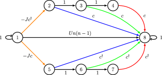
Figure 8: Finite state automaton used to construct the MPO tensor describing all the terms of the system Hamiltonian for a $3\times 3$ lattice with cylindrical boundary conditions. The coloured arrows represent different terms depending on the position of site $i$ relative to the lattice structure. The blue line represents the NN terms with the same x coordinate in the centre of the lattice. The green line represents the same NN term but around the PBC and the red lines are the NN terms with the same y-coordinate.

We explicitly write the MPO tensor corresponding to a top position in the lattice with the appropriate coefficients as

$$M^{i}=\left(\begin{array}[]{c|ccc|ccc|c}1&-Jc^{\dagger}&0&0&-Jc&0&0&Un(n-1)\\ \hline\cr&&1&&&&&e^{i2\pi x\phi}c\\ &&&1&&&&e^{-i2\pi x\phi}c\\ &&&&&&&c\\ \hline\cr&&&&&1&&e^{-i2\pi x\phi}c^{\dagger}\\ &&&&&&1&e^{i2\pi x\phi}c^{\dagger}\\ &&&&&&&c^{\dagger}\\ \hline\cr&&&&&&&1\end{array}\right),$$ (12)

where for the sake of visual order the empty terms in the matrix represent zeros. The dimension of the MPO is $2L_{y}+2$.

Appendix B Non-interacting ground state

We here describe how to obtain the analytical solution for the ground state of the system on the finite cylinder in the non-interacting limit $U=0$. We write the non-interacting Hamiltonian as

$$H=-J\bigg{[}\sum_{x=1}^{L_{x}-1}\sum_{y=1}^{L_{y}}c^{\dagger}_{x,y}c_{x+1,y}+\sum_{x=1}^{L_{x}}\bigg{(}e^{i2\pi x\phi}c^{\dagger}_{x,L_{y}}c_{x,1}\\ +\sum_{y=1}^{L_{y}-1}e^{i2\pi x\phi}c^{\dagger}_{x,y}c_{x,y+1}\bigg{)}\bigg{]}+\text{H.c.},$$ (13)

Because of the PBC in the $y$-direction we Fourier transform the bosonic operators as:

$$c_{m,n}=\frac{1}{L_{y}}\sum_{k}e^{ikn}c_{m,k},$$ (14)

where $k=2\pi n_{y}/L_{y}$ with $n_{y}=0,...,L_{y}-1$ are the discrete values of the momentum in $y$. In the mixed momentum and real space basis the Hamiltonian becomes

$$H=-J\sum_{x}\sum_{k}c^{\dagger}_{x,k}c_{x+1,k}+e^{-i2\pi x\phi}c^{\dagger}_{x,k}c_{x,k}+\text{H.c}.$$ (15)

Let us now consider a one-particle state with momentum $k$

$$\left|\psi(k)\right\rangle=\sum_{m}\psi_{m}(k)c^{\dagger}_{mk}\left|0\right\rangle.$$ (16)

By applying the Hamiltonian to the state the Schrödinger equation becomes

$$-J\big{(}\psi_{m+1}(k)+\psi_{m-1}(k)\big{)}-2J\cos(k+2\pi\phi m)\psi_{m}(k)=\\ E\psi_{m}(k).$$ (17)

By using the transfer matrix approach presented in Hatsugai (1993) we write Eq. 17 in matrix form as a recursive relation for the coefficients $\psi_{m}(k)$ as

$$\begin{pmatrix}\psi_{m+1}(k,\epsilon)\\ \psi_{m}(k,\epsilon)\end{pmatrix}=M_{m}(k,\epsilon)\begin{pmatrix}\psi_{m}(k,\epsilon)\\ \psi_{m-1}(k,\epsilon)\end{pmatrix},$$ (18)

where $\epsilon=E/J$ and

$$M_{m}(k,\epsilon)=\begin{pmatrix}-\epsilon-2\cos(k+2\pi\phi m)&-1\\ 1&0\end{pmatrix}.$$ (19)

The parameters of our system are: $L_{x}=9$, $L_{y}=6$ and $\phi=1/3$. Using the recursive relation in Eq. 18 we get

$$\begin{pmatrix}\psi_{10}(k,\epsilon)\\ \psi_{9}(k,\epsilon)\end{pmatrix}=\tilde{M}(k,\epsilon)\begin{pmatrix}\psi_{1}(k,\epsilon)\\ \psi_{0}(k,\epsilon)\end{pmatrix},$$ (20)

where

$$\tilde{M}(k,\epsilon)=M_{9}(k,\epsilon)M_{8}(k,\epsilon)\ldots M_{1}(k,\epsilon)=\\ \begin{pmatrix}\tilde{M}_{11}&\tilde{M}_{12}\\ \tilde{M}_{21}&\tilde{M}_{22}\end{pmatrix}.$$ (21)

For a fixed momentum value $k$, and fixing the boundary conditions as $\psi_{0}(k)=\psi_{10}(k)=0$ we obtain the eigenvalues of the problem by solving equation $\tilde{M}_{11}=0$. This is a polynomial of degree $9$ in $\epsilon$ whose roots give the energies of the eigenstates with momentum $k$. The ground state of the system is obtained by solving this equation for each value of $k$ and choosing the smallest root. Having fixed both $\bar{k}$ and chosen the ground state energy $\bar{\epsilon}$, we get the coefficients $\psi_{m}(\bar{k})$ of the ground state by using the recursive relation of Eq. 18. We find that for the ground state $\bar{\epsilon}\approx-2.6875$ and $\bar{k}=2\pi/3$. The ground state $\left|\bar{\psi}\right\rangle$ is written in real space as

$$\left|\bar{\psi}\right\rangle=\sum_{mn}\bar{\psi}_{m}e^{i2\pi n/3}c^{\dagger}_{mn}\left|0\right\rangle$$ (22)

where the $\bar{\psi}_{m}$ are such that the ground state function is normalized. We use this ground state function to calculate all the relevant observables. We find that

$$\langle n_{mn}\rangle=|\bar{\psi}_{m}|^{2},$$ (23)

$$\mathcal{I}^{y}(m)=2|\bar{\psi}_{m}|^{2}\sin(\frac{2\pi m}{3}+\frac{2\pi}{3}),$$ (24)

$$|C^{y}(m,n)|=1.$$ (25)

Our system is made of $9$ non-interacting bosons and they will all occupy the one-particle ground state. The many-particle ground state $\left|\bar{\Psi}\right\rangle$ is therefore

$$\left|\bar{\Psi}\right\rangle=\frac{1}{\sqrt{9}}\big{(}\sum_{mn}\bar{\psi}_{m}e^{i2\pi/3n}c^{\dagger}_{mn}\big{)}^{9}\left|0\right\rangle.$$ (26)

The expectation values for the density and current scale linearly with the number of particles whereas the correlation function does not because it is normalized. The results of the DMRG calculations are in agreement with the values obtained from this analysis.

References

- Cirac and Zoller (2012) J. I. Cirac and P. Zoller, “Goals and opportunities in quantum simulation,” Nat. Phys. 8, 264 (2012).
- Johnson et al. (2014) T. H. Johnson, S. R. Clark, and D. Jaksch, “What is a quantum simulator?” EPJ Quantum Technology 1, 10 (2014).
- Jaksch et al. (1998) D. Jaksch, C. Bruder, J. I. Cirac, C. W. Gardiner, and P. Zoller, “Cold bosonic atoms in optical lattices,” Phys. Rev. Lett. 81, 3108 (1998).
- Greiner et al. (2002) M. Greiner, O. Mandel, T. Esslinger, T. W. Hänsch, and I. Bloch, “Quantum phase transition from a superfluid to a Mott insulator in a gas of ultracold atoms,” Nature 415, 39 (2002).
- Bloch et al. (2008) I. Bloch, J. Dalibard, and W. Zwerger, “Many-body physics with ultracold gases,” Rev. Mod. Phys. 80, 885 (2008).
- Jördens et al. (2008) Robert Jördens, Niels Strohmaier, Kenneth Günter, Henning Moritz, and Tilman Esslinger, “A Mott insulator of fermionic atoms in an optical lattice,” Nature 455, 204–207 (2008).
- Gullans et al. (2012) M. Gullans, T. G. Tiecke, D. E. Chang, J. Feist, J. D. Thompson, J. I. Cirac, P. Zoller, and M. D. Lukin, “Nanoplasmonic lattices for ultracold atoms,” Phys. Rev. Lett. 109, 235309 (2012).
- Bakr et al. (2009) W. S. Bakr, J. I. Gillen, A. Peng, S. Fölling, and M. Greiner, “A quantum gas microscope for detecting single atoms in a Hubbard-regime optical lattice,” Nature 462, 74 (2009).
- Bakr et al. (2010) W. S. Bakr, A. Peng, M. E. Tai, R. Ma, J. Simon, J. I. Gillen, S. Fölling, L. Pollet, and M. Greiner, “Probing the superfluid-to-Mott insulator transition at the single-atom level,” Science 329, 547 (2010).
- Sherson et al. (2010) J. F. Sherson, C. Weitenberg, M. Endres, M. Cheneau, I. Bloch, and S. Kuhr, “Single-atom-resolved fluorescence imaging of an atomic Mott insulator,” Nature 467, 68 (2010).
- C. Weitenberg et al. (2011) C. Weitenberg, M. Endres, J. F. Sherson, M. Cheneau, P. Schauß, T. Fukuhara, I. Bloch, and S. Kuhr, “Single-spin addressing in an atomic Mott insulator,” Nature 471, 319 (2011).
- Gericke et al. (2008) T. Gericke, P. Würtz, D. Reitz, T. Langen, and H. Ott, “High-resolution scanning electron microscopy of an ultracold quantum gas,” Nat. Phys. 4, 949 (2008).
- Würtz et al. (2009) P. Würtz, T. Langen, T. Gericke, A. Koglbauer, and H. Ott, “Experimental demonstration of single-site addressability in a two-dimensional optical lattice,” Phys. Rev. Lett. 103, 080404 (2009).
- Cheuk et al. (2015) Lawrence W. Cheuk, Matthew A. Nichols, Melih Okan, Thomas Gersdorf, Vinay V. Ramasesh, Waseem S. Bakr, Thomas Lompe, and Martin W. Zwierlein, “Quantum-gas microscope for fermionic atoms,” Physical Review Letters 114, 193001 (2015).
- v. Klitzing et al. (1980) K. v. Klitzing, G. Dorda, and M. Pepper, “New method for high-accuracy determination of the fine-structure constant based on quantized Hall resistance,” Physical Review Letters 45, 494–497 (1980).
- Tsui et al. (1982a) D. C. Tsui, H. L. Stormer, and A. C. Gossard, “Two-dimensional magnetotransport in the extreme quantum limit,” Physical Review Letters 48, 1559–1562 (1982a).
- Tsui et al. (1982b) D. C. Tsui, H. L. Störmer, and A. C. Gossard, “Zero-resistance state of two-dimensional electrons in a quantizing magnetic field,” Phys. Rev. B 25, 1405–1407 (1982b).
- Jaksch and Zoller (2003) D Jaksch and P Zoller, “Creation of effective magnetic fields in optical lattices: the Hofstadter butterfly for cold neutral atoms,” New Journal of Physics 5, 56–56 (2003).
- Aidelsburger et al. (2013) M. Aidelsburger, M. Atala, M. Lohse, J. T. Barreiro, B. Paredes, and I. Bloch, “Realization of the Hofstadter hamiltonian with ultracold atoms in optical lattices,” Physical Review Letters 111, 185301 (2013).
- Miyake et al. (2013) Hirokazu Miyake, Georgios A. Siviloglou, Colin J. Kennedy, William Cody Burton, and Wolfgang Ketterle, “Realizing the Harper hamiltonian with laser-assisted tunneling in optical lattices,” Phys. Rev. Lett. 111, 185302 (2013).
- Aidelsburger et al. (2014) M. Aidelsburger, M. Lohse, C. Schweizer, M. Atala, J. T. Barreiro, S. Nascimbène, N. R. Cooper, I. Bloch, and N. Goldman, “Measuring the Chern number of Hofstadter bands with ultracold bosonic atoms,” Nature Physics 11, 162–166 (2014).
- Cooper and Dalibard (2013) N. R. Cooper and J. Dalibard, “Reaching fractional quantum Hall states with optical flux lattices,” Phys. Rev. Lett. 110, 185301 (2013).
- Cooper (2008) N.R. Cooper, “Rapidly rotating atomic gases,” Advances in Physics 57, 539–616 (2008).
- Harper et al. (2014) Fenner Harper, Steven H. Simon, and Rahul Roy, “Perturbative approach to flat Chern bands in the Hofstadter model,” Physical Review B 90, 075104 (2014).
- Scaffidi and Simon (2014) Thomas Scaffidi and Steven H. Simon, “Exact solutions of fractional Chern insulators: Interacting particles in the Hofstadter model at finite size,” Phys. Rev. B 90, 115132 (2014).
- Tai et al. (2017) M. Eric Tai, Alexander Lukin, Matthew Rispoli, Robert Schittko, Tim Menke, Dan Borgnia, Philipp M. Preiss, Fabian Grusdt, Adam M. Kaufman, and Markus Greiner, “Microscopy of the interacting Harper–Hofstadter model in the two-body limit,” Nature 546, 519–523 (2017).
- Hofstadter (1976) Douglas R. Hofstadter, “Energy levels and wave functions of Bloch electrons in rational and irrational magnetic fields,” Physical Review B 14, 2239–2249 (1976).
- Harper (1955) P G Harper, “The general motion of conduction electrons in a uniform magnetic field, with application to the diamagnetism of metals,” Proceedings of the Physical Society. Section A 68, 879–892 (1955).
- Hafezi et al. (2007) M. Hafezi, A. S. Sørensen, E. Demler, and M. D. Lukin, “Fractional quantum Hall effect in optical lattices,” Physical Review A 76, 023613 (2007).
- Laughlin (1983) R. B. Laughlin, “Anomalous quantum Hall effect: An incompressible quantum fluid with fractionally charged excitations,” Physical Review Letters 50, 1395–1398 (1983).
- Sørensen et al. (2005) Anders S. Sørensen, Eugene Demler, and Mikhail D. Lukin, “Fractional quantum Hall states of atoms in optical lattices,” Physical Review Letters 94, 086803 (2005).
- Möller and Cooper (2009) G. Möller and N. R. Cooper, “Composite fermion theory for bosonic quantum Hall states on lattices,” Phys. Rev. Lett. 103, 105303 (2009).
- Sterdyniak et al. (2012) Antoine Sterdyniak, Nicolas Regnault, and Gunnar Möller, “Particle entanglement spectra for quantum Hall states on lattices,” Physical Review B 86, 165314 (2012).
- White (1992) Steven R. White, “Density matrix formulation for quantum renormalization groups,” Physical Review Letters 69, 2863–2866 (1992).
- White (1993) Steven R. White, “Density-matrix algorithms for quantum renormalization groups,” Physical Review B 48, 10345–10356 (1993).
- Ciftja et al. (2011) Orion Ciftja, Nicole Ockleberry, and Chiko Okolo, “One-particle density of Laughlin states at finite n,” Modern Physics Letters B 25, 1983–1992 (2011).
- Rezayi and Haldane (1994) E. H. Rezayi and F. D. M. Haldane, “Laughlin state on stretched and squeezed cylinders and edge excitations in the quantum Hall effect,” Physical Review B 50, 17199–17207 (1994).
- Halperin (1982) B. I. Halperin, “Quantized Hall conductance, current-carrying edge states, and the existence of extended states in a two-dimensional disordered potential,” Physical Review B 25, 2185–2190 (1982).
- gang Wen (1992) Xiao gang Wen, “Theory of the edge states in fractional quantum Hall effects,” International Journal of Modern Physics B 06, 1711–1762 (1992).
- He et al. (2017) Yin-Chen He, Fabian Grusdt, Adam Kaufman, Markus Greiner, and Ashvin Vishwanath, “Realizing and adiabatically preparing bosonic integer and fractional quantum Hall states in optical lattices,” Physical Review B 96, 201103 (2017).
- Gerster et al. (2017) M. Gerster, M. Rizzi, P. Silvi, M. Dalmonte, and S. Montangero, “Fractional quantum Hall effect in the interacting Hofstadter model via tensor networks,” Physical Review B 96, 195123 (2017).
- Kitaev and Preskill (2006) Alexei Kitaev and John Preskill, “Topological entanglement entropy,” Phys. Rev. Lett. 96, 110404 (2006).
- Fendley et al. (2007) Paul Fendley, Matthew P. A. Fisher, and Chetan Nayak, “Topological entanglement entropy from the holographic partition function,” Journal of Statistical Physics 126, 1111–1144 (2007).
- Dong et al. (2008) Shiying Dong, Eduardo Fradkin, Robert G Leigh, and Sean Nowling, “Topological entanglement entropy in Chern-Simons theories and quantum Hall fluids,” Journal of High Energy Physics 2008, 016–016 (2008).
- Račiūnas et al. (2018) Mantas Račiūnas, F. N. Unal, Egidijus Anisimovas, and André Eckardt, “Creating, probing, and manipulating fractionally charged excitations of fractional chern insulators in optical lattices,” Phys. Rev. A 98, 063621 (2018).
- Budich et al. (2017) J. C. Budich, A. Elben, M. Łacki, A. Sterdyniak, M. A. Baranov, and P. Zoller, “Coupled atomic wires in a synthetic magnetic field,” Phys. Rev. A 95, 043632 (2017).
- Strinati et al. (2017) Marcello Calvanese Strinati, Eyal Cornfeld, Davide Rossini, Simone Barbarino, Marcello Dalmonte, Rosario Fazio, Eran Sela, and Leonardo Mazza, “Laughlin-like states in bosonic and fermionic atomic synthetic ladders,” Physical Review X 7, 021033 (2017).
- Petrescu et al. (2017) Alexandru Petrescu, Marie Piraud, Guillaume Roux, I. P. McCulloch, and Karyn Le Hur, “Precursor of the Laughlin state of hard-core bosons on a two-leg ladder,” Phys. Rev. B 96, 014524 (2017).
- Cincio and Vidal (2013) L. Cincio and G. Vidal, “Characterizing topological order by studying the ground states on an infinite cylinder,” Phys. Rev. Lett. 110, 067208 (2013).
- Nielsen et al. (2013) Anne E. B. Nielsen, Germán Sierra, and J. Ignacio Cirac, “Local models of fractional quantum Hall states in lattices and physical implementation,” Nature Communications 4, 2864 (2013).
- Bauer et al. (2014) Bela Bauer, Lukasz Cincio, Brendan P Keller, Michele Dolfi, Guifre Vidal, Simon Trebst, and Andreas WW Ludwig, “Chiral spin liquid and emergent anyons in a kagome lattice Mott insulator,” Nature communications 5, 5137 (2014).
- Tu et al. (2013) Hong-Hao Tu, Yi Zhang, and Xiao-Liang Qi, “Momentum polarization: An entanglement measure of topological spin and chiral central charge,” Physical Review B 88, 195412 (2013).
- Zaletel et al. (2013) Michael P Zaletel, Roger SK Mong, and Frank Pollmann, “Topological characterization of fractional quantum Hall ground states from microscopic hamiltonians,” Physical review letters 110, 236801 (2013).
- Łacki et al. (2016) Mateusz Łacki, Hannes Pichler, Antoine Sterdyniak, Andreas Lyras, Vassilis E. Lembessis, Omar Al-Dossary, Jan Carl Budich, and Peter Zoller, “Quantum Hall physics with cold atoms in cylindrical optical lattices,” Phys. Rev. A 93, 013604 (2016).
- Stoudenmire and White (2012) E.M. Stoudenmire and Steven R. White, “Studying two-dimensional systems with the density matrix renormalization group,” Annual Review of Condensed Matter Physics 3, 111–128 (2012).
- Crosswhite and Bacon (2008) Gregory M. Crosswhite and Dave Bacon, “Finite automata for caching in matrix product algorithms,” Phys. Rev. A 78, 012356 (2008).
- Al-Assam et al. (2017) S Al-Assam, S R Clark, and D Jaksch, “The tensor network theory library,” Journal of Statistical Mechanics: Theory and Experiment 2017, 093102 (2017).
- Vidal et al. (2003) G. Vidal, J. I. Latorre, E. Rico, and A. Kitaev, “Entanglement in quantum critical phenomena,” Phys. Rev. Lett. 90, 227902 (2003).
- Eisert et al. (2010) J. Eisert, M. Cramer, and M. B. Plenio, “Colloquium: Area laws for the entanglement entropy,” Reviews of Modern Physics 82, 277–306 (2010).
- Kol and Read (1993) A. Kol and N. Read, “Fractional quantum Hall effect in a periodic potential,” Physical Review B 48, 8890–8898 (1993).
- Jiang et al. (2012) Hong-Chen Jiang, Zhenghan Wang, and Leon Balents, “Identifying topological order by entanglement entropy,” Nature Physics 8, 902 (2012).
- Zhang et al. (2012) Yi Zhang, Tarun Grover, Ari Turner, Masaki Oshikawa, and Ashvin Vishwanath, “Quasiparticle statistics and braiding from ground-state entanglement,” Physical Review B 85, 235151 (2012).
- Hatsugai (1993) Yasuhiro Hatsugai, “Chern number and edge states in the integer quantum Hall effect,” Physical Review Letters 71, 3697–3700 (1993).